This article was downloaded by: [University of South Carolina ]On: 06 October 2013, At: 01:13Publisher: Taylor & FrancisInforma Ltd Registered in England and Wales Registered Number: 1072954 Registered office: Mortimer House,37-41 Mortimer Street, London W1T 3JH, UK

Structure and Infrastructure Engineering:Maintenance, Management, Life-Cycle Design andPerformancePublication details, including instructions for authors and subscription information:http://www.tandfonline.com/loi/nsie20

The risk-return tradeoff in optimizing regionalearthquake mitigation investmentNingxiong Xu a , Rachel A. Davidson a , Linda K. Nozick a & Atsuhiro Dodo ba School of Civil and Environmental Engineering, Hollister Hall, Cornell University, Ithaca,NY, 14853-3501, USb Swiss Reinsurance Company, 1-5-1 Otemachi, Chiyoda-ku, Tokyo, 100-0004, JapanPublished online: 16 Feb 2007.

To cite this article: Ningxiong Xu , Rachel A. Davidson , Linda K. Nozick & Atsuhiro Dodo (2007) The risk-return tradeoff inoptimizing regional earthquake mitigation investment, Structure and Infrastructure Engineering: Maintenance, Management,Life-Cycle Design and Performance, 3:2, 133-146, DOI: 10.1080/15732470600591083

To link to this article: http://dx.doi.org/10.1080/15732470600591083

PLEASE SCROLL DOWN FOR ARTICLE

Taylor & Francis makes every effort to ensure the accuracy of all the information (the “Content”) containedin the publications on our platform. However, Taylor & Francis, our agents, and our licensors make norepresentations or warranties whatsoever as to the accuracy, completeness, or suitability for any purpose of theContent. Any opinions and views expressed in this publication are the opinions and views of the authors, andare not the views of or endorsed by Taylor & Francis. The accuracy of the Content should not be relied upon andshould be independently verified with primary sources of information. Taylor and Francis shall not be liable forany losses, actions, claims, proceedings, demands, costs, expenses, damages, and other liabilities whatsoeveror howsoever caused arising directly or indirectly in connection with, in relation to or arising out of the use ofthe Content.

This article may be used for research, teaching, and private study purposes. Any substantial or systematicreproduction, redistribution, reselling, loan, sub-licensing, systematic supply, or distribution in anyform to anyone is expressly forbidden. Terms & Conditions of access and use can be found at http://www.tandfonline.com/page/terms-and-conditions

The risk-return tradeoff in optimizing regionalearthquake mitigation investment

NINGXIONG XU{, RACHEL A. DAVIDSON{, LINDA K. NOZICK*{ and ATSUHIRO DODO{

{School of Civil and Environmental Engineering, Hollister Hall, Cornell University,

Ithaca, NY 14853-3501, US

{Swiss Reinsurance Company, 1-5-1 Otemachi, Chiyoda-ku, Tokyo, 100-0004, Japan

(Received 13 April 2005; accepted in revised form 8 September 2005)

Earthquakes are low probability-high consequence events, regional earthquake miti-

gation is therefore a risky investment. Despite its importance, the risk-return tradeoff is

often not examined explicitly in regional earthquake risk management resource allocation

decisions. This paper introduces a stochastic optimization model developed to help

decision-makers understand the risk-return tradeoff in regional earthquake risk

mitigation, and to help state and local governments comply with the Disaster Mitigation

Act of 2000 requirement that they develop a mitigation plan. Taking advantage of the

special structure of the optimization, Dantzig-Wolfe decomposition is used as the solution

method. A case study for Central and Eastern Los Angeles illustrates an application of

the model. Results include a graph of the tradeoff between risk and return, quantification

of the relative contributions of each possible earthquake scenario, and discussion of the

effect of risk aversion on the selection of mitigation alternatives.

Keywords: Earthquakes; Optimization; Risk management; Resource allocation; Cost-

benefit analysis

1. Introduction

Earthquake mitigation analysis involves deciding: (1) how

much to spend on pre-event mitigation that aims to reduce

future earthquake losses versus post-event reconstruction

that aims to clean up after they occur, and (2) which of the

many possible mitigation alternatives to fund. This is an

investment problem in which one invests in mitigation

efforts (e.g. structural or non-structural upgrading of

certain types of structures in certain areas) at some cost,

and receives an uncertain return in the form of avoided

losses in the event of future earthquakes. The uncertainty

depends on which earthquakes occur in the future and

when. The problem is difficult in part because of the need to

tradeoff between the competing objectives of maximizing

the expected return on the investment and minimizing the

risk involved. While this tradeoff is true in any investment

situation, it is especially important in the case of investing

to mitigate earthquake losses because they are low

probability-high consequence events. There is a significant

earthquake risk-related benefit if a large earthquake occurs,

but there is none if no earthquake occurs (although there

may be other benefits, such as psychological benefits to

feeling safer or a reduction in vulnerability to other

hazards).

Despite its importance, the risk-return tradeoff often is

not systematically considered in earthquake mitigation

analysis. Ideally, all possible earthquakes with their

associated probabilities of occurrence would be considered

in estimating the benefits of possible mitigation invest-

ments. Almost all past studies, however, have calculated

benefits as those that would be realized if a particular

earthquake scenario occurred (e.g. Sarin 1983, Seligson

et al. 1998, Shah et al. 1992), or if the annual expected

ground shaking occurred (e.g. FEMA 1992, 1994, Altay

et al. 2002), because they are easier to calculate. Basing the

*Corresponding author. Email: lkn3@cornell.edu

Structure and Infrastructure Engineering, Vol. 3, No. 2, June 2007, 133 – 146

Structure and Infrastructure EngineeringISSN 1573-2479 print/ISSN 1744-8980 online ª 2007 Taylor & Francis

http://www.tandf.co.uk/journalsDOI: 10.1080/15732470600591083

Dow

nloa

ded

by [

Uni

vers

ity o

f So

uth

Car

olin

a ]

at 0

1:13

06

Oct

ober

201

3

benefit estimates on one, or even a few, scenarios is not

adequate, because what is an optimal investment strategy

for one earthquake is not necessarily optimal for all

earthquakes, and in fact can be completely ineffective

for other earthquakes, as demonstrated in Dodo et al.

(2005). Using the annual expected ground shaking is better

because it considers all possible earthquakes, but it does

not account for the spatial correlation among the benefits

associated with spatially distributed mitigation alternatives,

and therefore it does not consider the huge variability in

investment benefits. It assumes that a small loss (and

therefore mitigation benefit) occurs every year, whereas, in

reality, most years there will be no loss, but occasionally

there will be a very large loss.

This paper describes a new stochastic program developed

to support systematic regional earthquake mitigation

analysis with a specific focus on the risk-return tradeoff.

The variability in annual earthquake loss (and therefore net

benefit of mitigation investments) is explicitly modeled and

traded off with return on investment. The model was

developed with a focus on earthquakes and a regional

(e.g. metropolitan area) public sector perspective, but the

method could be adapted to other hazards and risk

management perspectives (e.g. insurance industry). This

work builds on that presented in Dodo et al. (2005). While

the model in Dodo et al. (2005) is similar in its definition of

mitigation alternatives and data sources, that model is a

linear program that focuses only on the expected value of

benefits. The stochastic program presented in this paper

makes the important extension to consider the variability in

benefits. The next section introduces relevant background

in resource allocation for natural disaster risk management.

Potential users and uses of the model are discussed,

followed by the model formulation and solution procedure,

and a case study application of the model for Eastern and

Central Los Angeles. The paper concludes with a discussion

of the model’s limitations and strengths.

2. Resource allocation for natural disaster risk management

Previous work relating to resource allocation for natural

disaster risk management can be grouped into four main

areas: (1) deterministic net present value (NPV) analysis,

(2) stochastic NPV analysis, (3) multi-attribute utility

models, and (4) optimization models. One of the key

dimensions used to distinguish studies is the way they

address the uncertainty related to earthquake (or other

hazard) occurrence. Only those studies categorized as

stochastic NPV studies recognize that in real life, future

benefits of mitigation investment are stochastic, and a

decision-maker may be interested not only in the expected

benefit, but the variability of benefits as well. Because

earthquakes are low probability-high consequence events,

the probability distribution of a NPV for earthquake

investments has a large variance. There is a small

probability that a major earthquake will occur and large

losses will be avoided, and a large probability that no

earthquake will occur, resulting in no investment benefit.

Therefore, risk managers probably do not want to make

decisions based solely on expected values.

Few stochastic NPV studies could be found in the

literature. Englehardt and Peng (1996) estimated the

probability distribution of benefits associated with revising

the hurricane requirements in a South Florida building

code, and compared it with the cost of implementing the

revision. Bernknopf et al. (2001) applied a stochastic NPV

analysis to lateral-spread ground failure in Watsonville,

CA, assuming the 1989 Loma Prieta earthquake may or

may not occur again. They compared two mitigation

alternatives: to mitigate all properties in a particular land

use class, or all properties in a particular hazard class. The

two alternatives were compared based on the mean and

variance of the NPV. Taylor and Werner (1995), Werner

et al. (1999), and Werner et al. (2002) compare various

levels of proposed seismic design or upgrade for port

facilities in California based on both means and standard

deviations of losses. Mostafa and Grigoriu (2002) examined

the benefits of adding bracing elements to the water tank in

a New York City hospital. One thousand seismic events

were generated stochastically, and the distributions of

losses with and without mitigation were compared.

The authors are aware of only one example in which

stochastic analysis was used in an optimization approach

for resource allocation for natural disaster risk manage-

ment. Researchers at the International Institute for

Applied Systems Analysis (IIASA) developed a simulation-

optimization approach to select the insurance policy design

(e.g. insurance premiums) that best satisfies stated decision

criteria, such as maximizing insurance company profits and

minimizing the probability of insurance company insol-

vency (Ermoliev et al. 2000). The problem they address is

heavily focused on financial instruments, and their for-

mulation yields an intractable analytical structure for the

objective. They rely, therefore on simulation for their

analysis. Our model centers on mitigation decisions and a

public decision-making perspective. This yields a very

different model formulation, one with a much closer tie

to regional loss estimation methodologies. The structure of

this model makes it amenable to analytic analysis.

3. Potential model users and uses

The stochastic program presented in this paper was

developed with a local (e.g. county) public sector perspec-

tive because mitigation is largely a local issue (Prater and

Lindell 2000). Although the mitigation planning process

involves complicated interactions among multiple layers of

government, local governments play a key role since most

134 N. Xu et al.

Dow

nloa

ded

by [

Uni

vers

ity o

f So

uth

Car

olin

a ]

at 0

1:13

06

Oct

ober

201

3

infrastructure is controlled by local governments, residents,

and businesses (not the state or federal government) and

regulations governing land use and construction practices

are established at the local level (Prater and Lindell 2000).

As with most computer models, this optimization model

does not capture all the complexities of the social, political,

economic, and cultural context in which resource allocation

decisions are actually made. Nevertheless, it should provide

useful input to support the mitigation planning process.

Running the model under different assumptions could help

decision-makers understand how the many relevant factors

(e.g. distribution of earthquake ground shaking, structural

vulnerability, objectives, mitigation alternative costs, risk

attitudes) interact to determine the relative appeal of different

mitigation strategies. The model’s solutions can also provide

insight into which strategy is optimal for a given community.

In addition to general earthquake risk reduction resource

allocation support, the model aims to help local and state

risk managers undertake a few specific mitigation planning

tasks. The Disaster Mitigation Act of 2000 now requires

that to be eligible for Hazard Mitigation Grant Program

(HMGP) funds, each state and local government must

submit a mitigation plan to the Federal Emergency

Management Agency (FEMA) describing how it is

prioritizing mitigation actions so that its overall mitigation

strategy is cost-effective and maximizes overall wealth

(FEMA 2002, 2003). The model could provide guidance as

governments respond to this mandate. After an earth-

quake, many applications for HMGP grants are submitted,

and need to be evaluated quickly and rationally. By

systematically comparing regional strategies (e.g. upgrade

all unreinforced masonry buildings in a census tract), the

model can help streamline administration of the HMGP by

providing a mechanism for ‘block grant’ approval, just as

the RAMP program did after the 1994 Northridge earth-

quake (Seligson et al. 1998). The Small Business

Administration’s Pre-Disaster Mitigation Loan Program

makes low-interest, fixed-rate loans to small businesses so

they can implement mitigation measures. To be eligible, the

business must ‘conform to the priorities and goals of the

mitigation plan for the community, as defined by FEMA,

in which the business is located’ (US SBA 2003). The model

could help the local or state mitigation official decide which

applications to approve.

4. Model formulation

4.1 Scope

The model was designed to be compatible with HAZUS,

the Federal Emergency Management Agency’s publicly-

available, standardized national loss estimation modeling

software, so that HAZUS could be used to calculate

regional earthquake losses (benefits of investment) when

necessary (FEMA 1999). The mitigation alternatives

considered in the model are structural upgrading policies

for groups of buildings. Buildings are grouped into

categories based on their census tract locations, structural

types (e.g. mid-rise steel braced frame, low-rise concrete

shear wall), occupancy types (e.g. single-family dwelling,

hospital), and design levels (i.e. built to a low, moderate, or

high seismic code). One mitigation alternative considered is

to upgrade some square footage of buildings of a particular

structural and occupancy type in a census tract from one

design level to another. The set of mitigation alternatives

considered is created by all possible combinations of

structural types, occupancy types, census tracts, and design

levels. In reality, it is possible to mitigate a single structure

in many ways. There are other possible combinations of

structures that could be mitigated, instead of buildings in

a census tract. The unit of census tract is used because it is

the smallest one available in HAZUS (FEMA 1999), but

another area unit, such as block group, could be used

without altering the model formulation. Square footage was

chosen as the metric of study because HAZUS uses square

footage (FEMA 1999), not the number of buildings, to

calculate loss. From a computational perspective, modeling

the decision variables as continuous variables (square

footage) instead of integers (number of buildings) produces

a much simpler and more appropriate optimization for the

level of data which is available for a regional planning

investment analysis. There are also many non-structural

mitigation alternatives, such as land use planning or buying

insurance. This model does not currently allow these types of

alternatives, though they could be incorporated. Except

mitigation costs, all input for the model can be obtained

from any regional loss estimation model, such as HAZUS.

In the next section, the definition of risk used in this study is

presented, and in the subsequent section, the equations that

make up the stochastic program are developed.

4.2 Measuring risk

Bawa (1975) and Fishburn (1977) discuss ‘downside risk’

in the context of a financial investment portfolio. They

measure risk as a lower partial moment (LPM) of order brelative to the minimum acceptable rate of return, a,defined as follows:

LPMbða;RÞ ¼Z a

�1ða� RÞb dFðRÞ; ð1Þ

where F(R) is the cumulative distribution function of the

uncertain rate of return, R. The key point is the focus on a

‘one-sided’ risk measure rather than on variance. In this

earthquake risk management problem, we want to avoid

the possibility of experiencing losses that exceed some

allowable threshold value, defined such that earthquake

loss less than that level is viewed as within the regional

Risk-return tradeoff in mitigation 135

Dow

nloa

ded

by [

Uni

vers

ity o

f So

uth

Car

olin

a ]

at 0

1:13

06

Oct

ober

201

3

capacity to manage it, and loss greater than that level is

not. At the same time, we want to achieve a solution that is

good in an expected value sense. To accomplish this, we

develop a variation on the idea described by Bawa (1975)

and Fishburn (1977) that focuses on an ‘upper partial

moment’ of order 1, i.e. the partial expectation of loss

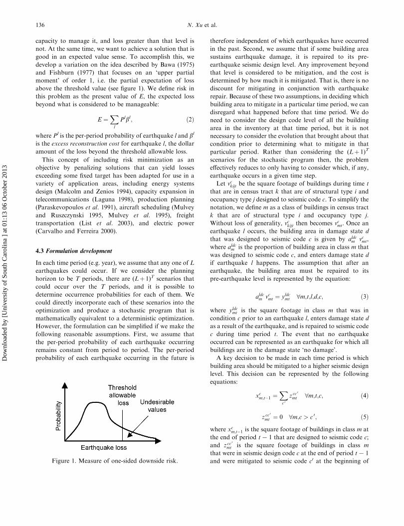
above the threshold value (see figure 1). We define risk in

this problem as the present value of E, the expected loss

beyond what is considered to be manageable:

E ¼Xl

Plbl; ð2Þ

where Pl is the per-period probability of earthquake l and bl

is the excess reconstruction cost for earthquake l, the dollar

amount of the loss beyond the threshold allowable loss.

This concept of including risk minimization as an

objective by penalizing solutions that can yield losses

exceeding some fixed target has been adapted for use in a

variety of application areas, including energy systems

design (Malcolm and Zenios 1994), capacity expansion in

telecommunications (Laguna 1998), production planning

(Paraskevopoulos et al. 1991), aircraft scheduling (Mulvey

and Ruszczynski 1995, Mulvey et al. 1995), freight

transportation (List et al. 2003), and electric power

(Carvalho and Ferreira 2000).

4.3 Formulation development

In each time period (e.g. year), we assume that any one of L

earthquakes could occur. If we consider the planning

horizon to be T periods, there are (Lþ 1)T scenarios that

could occur over the T periods, and it is possible to

determine occurrence probabilities for each of them. We

could directly incorporate each of these scenarios into the

optimization and produce a stochastic program that is

mathematically equivalent to a deterministic optimization.

However, the formulation can be simplified if we make the

following reasonable assumptions. First, we assume that

the per-period probability of each earthquake occurring

remains constant from period to period. The per-period

probability of each earthquake occurring in the future is

therefore independent of which earthquakes have occurred

in the past. Second, we assume that if some building area

sustains earthquake damage, it is repaired to its pre-

earthquake seismic design level. Any improvement beyond

that level is considered to be mitigation, and the cost is

determined by how much it is mitigated. That is, there is no

discount for mitigating in conjunction with earthquake

repair. Because of these two assumptions, in deciding which

building area to mitigate in a particular time period, we can

disregard what happened before that time period. We do

need to consider the design code level of all the building

area in the inventory at that time period, but it is not

necessary to consider the evolution that brought about that

condition prior to determining what to mitigate in that

particular period. Rather than considering the (Lþ 1)T

scenarios for the stochastic program then, the problem

effectively reduces to only having to consider which, if any,

earthquake occurs in a given time step.

Let vckijt be the square footage of buildings during time t

that are in census tract k that are of structural type i and

occupancy type j designed to seismic code c. To simplify the

notation, we define m as a class of buildings in census tract

k that are of structural type i and occupancy type j.

Without loss of generality, vckijt then becomes vcmt. Once an

earthquake l occurs, the building area in damage state d

that was designed to seismic code c is given by aldcm vcmt,

where aldcm is the proportion of building area in class m that

was designed to seismic code c, and enters damage state d

if earthquake l happens. The assumption that after an

earthquake, the building area must be repaired to its

pre-earthquake level is represented by the equation:

aldcm vcmt ¼ yldcmt 8m;t;l;d;c; ð3Þ

where yldcmt is the square footage in class m that was in

condition c prior to an earthquake l, enters damage state d

as a result of the earthquake, and is repaired to seismic code

c during time period t. The event that no earthquake

occurred can be represented as an earthquake for which all

buildings are in the damage state ‘no damage’.

A key decision to be made in each time period is which

building area should be mitigated to a higher seismic design

level. This decision can be represented by the following

equations:

xcm;t�1 ¼Xc 0

z cc0

mt 8m;t;c; ð4Þ

z cc0

mt ¼ 0 8m;c > c 0; ð5Þ

where xcm;t�1 is the square footage of buildings in class m at

the end of period t7 1 that are designed to seismic code c;

and z cc0

mt is the square footage of buildings in class m

that were in seismic design code c at the end of period t7 1

and were mitigated to seismic code c0 at the beginning ofFigure 1. Measure of one-sided downside risk.

136 N. Xu et al.

Dow

nloa

ded

by [

Uni

vers

ity o

f So

uth

Car

olin

a ]

at 0

1:13

06

Oct

ober

201

3

period t. Mitigation has occurred only when c04 c. If c0 ¼ c,

no mitigation has occurred, but the square footage is

conserved at zero mitigation cost. The following relation-

ship must hold between the z and n variables:

v c0

mt ¼Xc

z cc0

mt 8m;t;c 0: ð6Þ

Equation (6) requires that the square footage in building

class m in time period t designed to seismic code c0 equals

the square footage that has been mitigated to that seismic

code during t. The square footage of buildings in class m at

the end of period t that are designed to seismic code c is

then given by:

xcmt ¼ vcmt 8m;t;c: ð7Þ

Finally, the desire to guard against scenarios that would

produce losses greater than a specified allowable threshold

level is represented by the following constraint:Xm

Xd

Xc

Rdcmty

ldcmt � blt � Bt 8l;t; ð8Þ

where Rdcmt is the per square foot reconstruction cost for

building area in class m that enters damage state d and is

repaired to code c during period t; Bt is the allowable loss in

period t, the dollar loss that is considered manageable in

period t; and blt is the excess reconstruction cost for

earthquake l and period t, the dollar amount of the loss

beyond this allowable loss threshold in period t. The

following non-negativity requirements must also hold:

blt � 0 8l;t; ð9Þ

xcmt;vcmt � 0 8m;t;c; ð10Þ

z cc0

mt � 0 8m;t;c;c 0; ð11Þ

yldcmt � 0 8m;t;l;d;c: ð12Þ

We can now develop a multi-objective optimization

formulation in which the tradeoff between two objectives is

represented with a weight k. One objective is to minimize

the present value of the sum of the mitigation investment

and the expected reconstruction expenditures. The second

objective is to minimize the present value of the risk, as

defined in equation (2). The objective function is as follows:

minXt

1

1þ rð Þt�1

�Xm

Xc

Xc 0

Fcc 0

mt zcc 0

mt

þXm

Xc

Xl

Xd

PlRdcmty

ldcmt þ k

Xl

Plblt

�; ð13Þ

where k� 0 is the weight for the risk-based objective; Fcc 0

mt is

the per square foot cost to upgrade building area in class m

from seismic code c to code c0 in time period t; and r is an

interest rate per period used to discount cash flows to the

present value. A higher value of k represents more risk

aversion. The final optimization model is a linear program

in which the objective is given in equation (13) and the

constraints are given in equations (3) – (12). The model

results indicate what the total mitigation and expected post-

earthquake reconstruction costs will be, as well as the risk

associated with the mitigation strategy, in terms of the

expected excess reconstruction cost over all possible earth-

quakes during the time horizon.

The optimization model requires seven key inputs:

(1) xcm0, the inventory at time 0; (2) aldcm , the proportion of

building area in class m that was designed to seismic code c

and enters damage state d after an earthquake l; (3) Rdcmt, the

per square foot reconstruction cost for building area in

class m that enters damage state d and is repaired to code c

during period t; (4) Fcc 0

mt , the per square foot cost to upgrade

the building area in class m from seismic code c to code c0 in

period t; (5) Pl, the per-period probability of earthquake l;

(6) Bt, the user-defined allowable loss in each period t; and

(7) k, the user-defined weight used to tradeoff between the

two objectives. Items 1 to 3 can be obtained from any

regional loss estimation model. For items 6 and 7, it may be

difficult to define ‘the’ values of allowable loss and risk

aversion weight that represent a community’s interests. It

can be valuable, nonetheless, to run the analyses with

several possible values of allowable loss and risk aversion

weights, and examine the effects of these variables on the

recommended mitigation plan.

5. Model simplification

Realistic applications of this formulation include a very

large number of decision variables. For example, the case

study described in this paper, which focuses on 86 square

miles in the City of Los Angeles, yields a formulation with

over 11.1 million variables (after some substitution). Any

reduction in the size of the formulation, is therefore

helpful in making the model more useful for real-life

applications. It turns out that with two reasonable

assumptions, it can be shown that mitigation expenditures

are made only in the first period, which implies that the

formulation can be reduced to a one-period problem in

which the benefits and costs that stem from those

investments are calculated over the planning horizon. This

simplification dramatically reduces the computation re-

quired to solve the model. The assumptions are: (1) that

mitigating from low to medium code, then from medium

to high code is at least as expensive as mitigating directly

from low to high code (the condition is more general if

there are more than three code levels); and (2) that all

mitigation and reconstruction cost coefficients are

stationary (i.e. do not change over time). The theorem

connecting these assumptions to a one-period model

Risk-return tradeoff in mitigation 137

Dow

nloa

ded

by [

Uni

vers

ity o

f So

uth

Car

olin

a ]

at 0

1:13

06

Oct

ober

201

3

formulation is proved in Appendix I. The resulting

simplified model formulation is presented in this section.

Equation (14) links the initial square footage in class m

that was designed to seismic code c to the mitigation

decisions for that class and initial seismic design code.

Equation (15) calculates bl, the reconstruction cost in excess

of the allowable loss for each potential earthquake l. The

first term on the left side is the reconstruction cost if

earthquake l occurs, given the mitigation decisions that

have been made. Mitigation can only improve the seismic

design code of a building, so equation (16) must hold. The

non-negativity requirements in equations (17) and (18)

must also hold:

xcm ¼Xc 0

z cc0

m 8m;c; ð14Þ

Xm;c 0;d

Rdc 0

m aldc0

m

Xc

z cc0

m � bl � B 8l; ð15Þ

z cc0

m ¼ 0 8m; c > c 0; ð16Þ

bl � 0 8l; ð17Þ

z cc0

m � 0 8m;c;c 0: ð18Þ

The objective function in equation (13) can now be

simplified as follows:

minXm

Xc

Xc 0

Fcc 0

m þXl

Xd

dPlaldc0

m Rdc 0

m

!z cc

0

m

þ kdXl

Plbl; ð19Þ

where d ¼ 1þrr

�1�

�1

1þr�T�

and T is the number of periods

in the planning horizon. The other variables in equations

(14) – (19) are the same as defined previously, but without

the time index. These simplifications drastically reduce the

size of the formulation. Considering again the case study in

this paper, the simplified formulation has only 369,000

variables, compared to over 11.1 million variables in the

original formulation.

6. Dantzig-Wolfe solution procedure

Even the one-period model formulation can lead to very

large problems in realistic instances. An analysis for the

entire City of Los Angeles, for example, requires 2.2 million

variables in the simplified formulation (65 million in the

original version). However, the formulation has a special

structure that can be exploited to create an efficient solution

procedure. Notice that if equation (15) were removed, the

formulation would decompose into m*c independent linear

programs. This circumstance suggests that a Dantzig-Wolfe

decomposition (Bertsimas and Tsitsiklis 1977) is an

appropriate solution procedure. The idea of a Dantzig-

Wolfe decomposition is that rather than representing the

impact of each of these independent linear programs on the

optimization through the constraints, as in the formulation

above, one can explicitly use the set of extreme points to

define the feasible region generated by the constraints.

Since the feasible region of a bounded linear program is a

convex set, any feasible point can be represented as a

convex combination of the extreme points in that set. For

the purposes of this discussion, we assume the feasible

region is bounded because our formulation is bounded and

hence, we need not consider extreme directions.

A Dantzig-Wolfe decomposition specifies the use of a

master problem and a series of sub-problems. There is one

sub-problem for each class m and initial seismic design

code c. The master problem is comprised of the linking

constraints and a collection of additional variables that

represent a subset of the extreme points of each of the sub-

problems. At each iteration, a new extreme point is

generated for each of the sub-problems and these are

added to the master problem. The algorithm terminates

when the optimal solution has been identified. That optimal

solution is expressed as a convex combination of the

extreme points that satisfy the linking constraints.

The algorithm is described in the following five steps.

First, for all m and c, let z1ccm ¼ xcm, and for all c0 6¼ c let

z1cc0

m ¼ 0. This initial solution for each of the sub-problems

corresponds to no mitigation. The notation zncc0

m is the nth

solution to the sub-problem of how to optimally mitigate

the square footage in class m with initial seismic code c.

Second, at iteration n, there are n extreme points

zhcc0

m : 8m;c;c 0�

for h¼ 1, . . . , n. Solve the following

restricted master program to obtain the optimal yh for

h¼ 1, . . . , n and to obtain the dual prices pl correspondingto constraint (21) and r corresponding to constraint (22):

minXnh¼1

Xm

Xc

Xc 0

Fcc 0

m þXl

Xd

dPlaldc0

m Rdc 0

m

!zhcc

0

m yh

þ kdXl

Plbl; ð20Þ

subject to:Xnh¼1

Xm

Xc

Xc 0

Xd

aldc0

m Rdc 0

m zhcc0

m yh � bl � B 8l;

ð21Þ

Xnh¼1

yh ¼ 1; ð22Þ

bl � 0 8l; ð23Þ

yh � 0 8h: ð24Þ

138 N. Xu et al.

Dow

nloa

ded

by [

Uni

vers

ity o

f So

uth

Car

olin

a ]

at 0

1:13

06

Oct

ober

201

3

The mitigation strategy recommended by the master

problem at the nth iteration is then a convex combination

of the mitigation decisions identified in each of the n

iterations for each sub-problem where the weights for that

combination are given by yh. Third, for each class m and

initial seismic code c, find c0 � c to minimize

Fcc 0

m þP

d

Pl dPl � pl� �

aldc0

m Rdc 0

m . Assume that c� achieves

the minimum. Fourth, define a new extreme point of

equations (14), (16) and (18) as follows: znþ1;cc�m ¼ xcm and

znþ1;cc0

m ¼ 0 for c 0 6¼ c�, 8m;c;c 0. It is important to remember

that c� is defined for each class m and initial seismic code c.

We have suppressed the notion that c� is a function of m

and c to simplify the discussion. Fifth, if the following is

true,

Xm

Xc

F cc�m þ

Xd

Xl

dPl � pl� �

aldc�m Rdc�m

!xcm � r; ð25Þ

the optimal solution found on the previous iteration of the

restricted master problem is the optimal for the problem.

That solution is given byPn

k¼1 zhcc 0

m yh. If this condition is

not true, the solutions to the sub-problems that have just

been identified and are given by znþ1;cc0

m 8m;c;c 0, are added

to the restricted master problem and the process continues

by returning to step 2. Note that the objective value of the

restricted master program is non-increasing at each

iteration and that each of these solutions is a feasible

solution to the original optimization. In practice, the

termination criteria used for Dantzig-Wolfe are: (1) the

optimality condition that is given by equation (25) for this

formulation; (2) a specified maximum number of iterations;

or (3) the condition that the value of the left side of the

optimality condition is less than r, but by what is deemed

to be a very small amount.

7. Case study

7.1 Scope

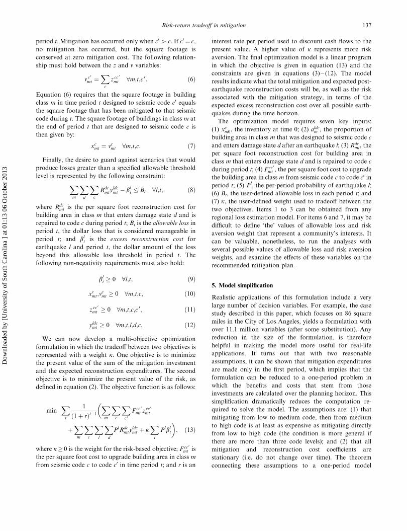
A case study analysis was conducted for the Central and

Eastern part of the City of Los Angeles, as defined by the

Los Angeles Area Planning Commission (LADRU 2004),

see figure 2. This diverse area of 86 square miles includes

Hollywood, Wilshire, Westlake, Silver Lake-Echo Park,

Central City, Central City North, Boyle Heights, and

Northeast Los Angeles. HAZUS was used as the basis for

most of the required data. HAZUS defines 36 structural

types (e.g. mid-rise steel braced frame, low-rise concrete

shear wall) and 28 occupancy types (e.g. single-family

dwelling, hospital) (FEMA 1999). There were 11 structural

types and 17 occupancy types in the 201 census tracts that

make up this case study area.

Table 1 lists the floor area in the region by structural

type. Within these 201 census tracts, there are about 167

million square foot of building space, of which about 16%,

56%, and 28% are designed to low, moderate, and high

seismic code, respectively. The most prevalent occupancy

types are multi-family dwelling (RES3), wholesale trade

(COM2), and retail trade (COM1), which make up 28%,

17%, and 15% of the building area, respectively. The

census tracts with the most square footage are those around

the Central City North area. The case study considered the

same 3 design levels (built to low, moderate, high seismic

design code), and the same 5 damage states (no, slight,

moderate, extensive, and complete damage) defined by

HAZUS (FEMA 1999). Structural, non-structural, con-

tents, inventory, and time-related losses are considered in

the estimation of reconstruction costs, but not for example,

indirect economic or human life losses. Time-related losses

include relocation expenses, loss of proprietor’s income,

rental income loss, and inventory loss.

Figure 2. Case study census tract locations in Los Angeles County.

Risk-return tradeoff in mitigation 139

Dow

nloa

ded

by [

Uni

vers

ity o

f So

uth

Car

olin

a ]

at 0

1:13

06

Oct

ober

201

3

7.2 Input data

In the case study analysis, the regional seismicity was

assumed to be represented by the set of 47 earthquake

scenarios identified by Chang et al. (2000) for a risk

analysis of the highway network in Los Angeles and

Orange Counties. The analysis thus assumes that only those

47 earthquakes are possible, each with an associated annual

‘hazard-consistent’ probability of occurrence, such that

together they approximate the regional seismicity. The

‘hazard-consistent’ probability of a particular earthquake

scenario represents the likelihood of earthquakes like that

scenario occurring, where ‘earthquakes like that scenario’

are similar in terms of severity and spatial distribution of

ground motion they cause (Chang et al. 2000). In this way,

all earthquakes are considered.

It was assumed that the time step is 1 year, the valuation

period is 30 years, the annual interest rate is 2%, and the

allowable loss is B¼ $1 billion. The analysis was conducted

for many values of the risk aversion weight, k. The case

study uses HAZUS default inventory data, which is from

1994 (FEMA 1999). The mitigation costs (Fcc 0

mt ) and

reconstruction costs (based on adcm and Rdcc 0

mt ) were estimated

based on information from HAZUS data tables and

simulation results, as described in Dodo et al. (2005).

Mitigation and reconstruction costs are estimated for the

year 2003.

7.3 Case study results

The solution algorithm was programmed in C. The

optimization model results can provide a risk manager

with guidance on specific earthquake risk resource alloca-

tion decisions, such as those described in the Potential

Model Users and Uses section, and can also help him or

her gain general insight into the risk-return tradeoff.

The results can be used to answer many questions,

including: (1) How do expected expenditures vary with

risk attitude? (2) What is the relative contribution of the

different possible earthquakes to exceeding allowable loss?

(3) Does the recommended mitigation strategy vary with

risk attitude? These questions are examined for the case

study analysis in turn in the following sections.

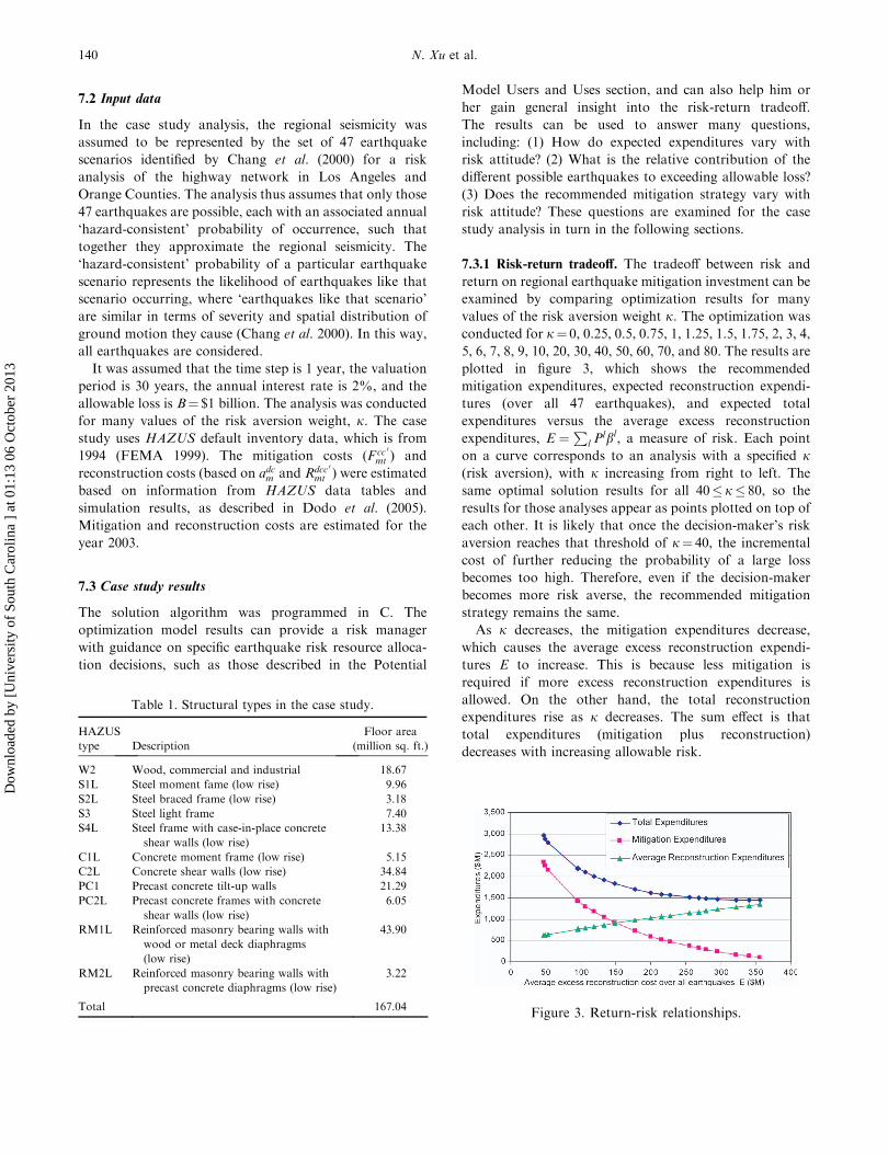
7.3.1 Risk-return tradeoff. The tradeoff between risk and

return on regional earthquake mitigation investment can be

examined by comparing optimization results for many

values of the risk aversion weight k. The optimization was

conducted for k¼ 0, 0.25, 0.5, 0.75, 1, 1.25, 1.5, 1.75, 2, 3, 4,

5, 6, 7, 8, 9, 10, 20, 30, 40, 50, 60, 70, and 80. The results are

plotted in figure 3, which shows the recommended

mitigation expenditures, expected reconstruction expendi-

tures (over all 47 earthquakes), and expected total

expenditures versus the average excess reconstruction

expenditures, E ¼P

l Plbl, a measure of risk. Each point

on a curve corresponds to an analysis with a specified k(risk aversion), with k increasing from right to left. The

same optimal solution results for all 40� k� 80, so the

results for those analyses appear as points plotted on top of

each other. It is likely that once the decision-maker’s risk

aversion reaches that threshold of k¼ 40, the incremental

cost of further reducing the probability of a large loss

becomes too high. Therefore, even if the decision-maker

becomes more risk averse, the recommended mitigation

strategy remains the same.

As k decreases, the mitigation expenditures decrease,

which causes the average excess reconstruction expendi-

tures E to increase. This is because less mitigation is

required if more excess reconstruction expenditures is

allowed. On the other hand, the total reconstruction

expenditures rise as k decreases. The sum effect is that

total expenditures (mitigation plus reconstruction)

decreases with increasing allowable risk.

Table 1. Structural types in the case study.

HAZUS

type Description

Floor area

(million sq. ft.)

W2 Wood, commercial and industrial 18.67

S1L Steel moment fame (low rise) 9.96

S2L Steel braced frame (low rise) 3.18

S3 Steel light frame 7.40

S4L Steel frame with case-in-place concrete

shear walls (low rise)

13.38

C1L Concrete moment frame (low rise) 5.15

C2L Concrete shear walls (low rise) 34.84

PC1 Precast concrete tilt-up walls 21.29

PC2L Precast concrete frames with concrete

shear walls (low rise)

6.05

RM1L Reinforced masonry bearing walls with

wood or metal deck diaphragms

(low rise)

43.90

RM2L Reinforced masonry bearing walls with

precast concrete diaphragms (low rise)

3.22

Total 167.04Figure 3. Return-risk relationships.

140 N. Xu et al.

Dow

nloa

ded

by [

Uni

vers

ity o

f So

uth

Car

olin

a ]

at 0

1:13

06

Oct

ober

201

3

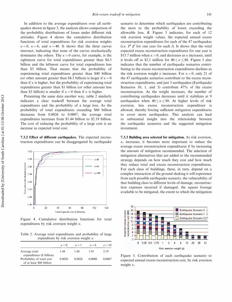
In addition to the average expenditures over all earth-

quakes shown in figure 3, the analysis allows comparison of

the probability distributions of losses under different risk

attitudes. Figure 4 shows the cumulative distribution

functions of total expenditures for risk aversion weights

k¼ 0, k¼ 6, and k¼ 40. It shows that the three curves

intersect, indicating that none of the curves stochastically

dominates the others. The k¼ 0 curve, for example, is the

rightmost curve for total expenditures greater than $4.5

billion and the leftmost curve for total expenditures less

than $3 billion. That means that the probability of

experiencing total expenditures greater than $40 billion

(or other amount greater than $4.5 billion) is larger if k¼ 0

than if k is higher, but the probability of experiencing total

expenditures greater than $1 billion (or other amount less

than $3 billion) is smaller if k¼ 0 than if k is higher.

Presenting the same data another way, table 2 similarly

indicates a clear tradeoff between the average total

expenditures and the probability of a large loss. As the

probability of total expenditures exceeding $60 billion

decreases from 0.0026 to 0.0007, the average total

expenditures increases from $1.44 billion to $2.19 billion.

The cost of reducing the probability of a large cost is an

increase in expected total cost.

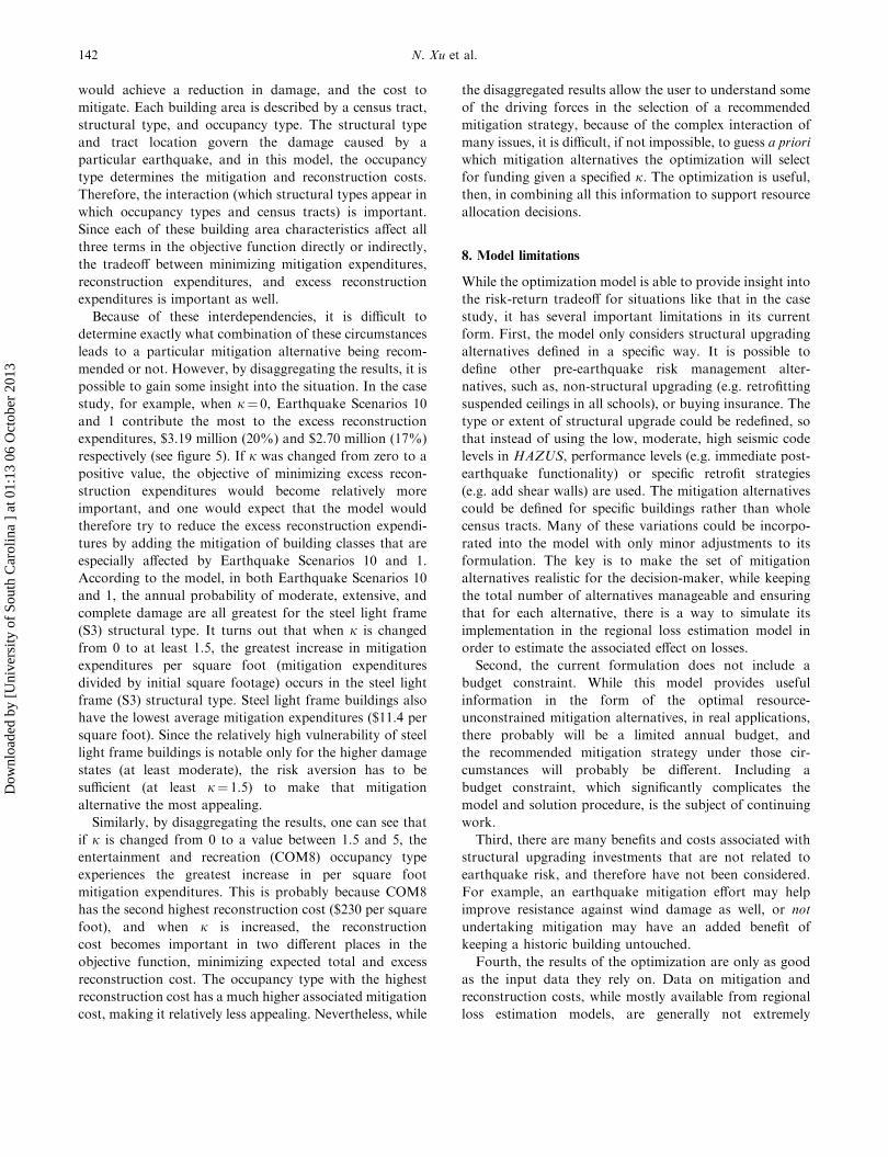
7.3.2 Effect of different earthquakes. The expected recons-

truction expenditures can be disaggregated by earthquake

scenario to determine which earthquakes are contributing

the most to the probability of losses exceeding the

allowable loss, B. Figure 5 indicates, for each of 12

risk aversion weight values, the expected annual excess

reconstruction expenditures for each of the 47 earthquakes

(i.e. Pl bl for one year for each l). It shows that the total

expected excess reconstruction expenditures for one year is

$15.7 million when k¼ 0, and decreases as k increases, until

it levels off at $2.1 million for 40�k� 80. Figure 5 also

indicates that the number of earthquake scenarios contri-

buting to the excess reconstruction expenditures declines as

the risk aversion weight k increases. For k¼ 0, only 21 of

the 47 earthquake scenarios contribute to the excess recon-

struction expenditures, and just 3 earthquakes (Earthquake

Scenarios 10, 1, and 3) contribute 47% of the excess

reconstruction. As the weight increases, the number of

contributing earthquakes decreases until it stabilizes at 9

earthquakes when 40� k� 80. At higher levels of risk

aversion, less excess reconstruction expenditure is

allowed, thereby forcing sufficient mitigation expenditures

to cover more earthquakes. This analysis can lead

to substantial insight into the relationship between

the earthquake scenarios and the suggested mitigation

investment.

7.3.3 Building area selected for mitigation. As risk aversion,

k, increases, it becomes more important to reduce the

average excess reconstruction expenditures E by increasing

the amount of mitigation recommended. The selection of

mitigation alternatives that are added to the recommended

strategy depends on how much they cost and how much

they reduce total and excess reconstruction expenditures.

For each class of buildings, these, in turn, depend on a

complex interaction of the ground shaking it will experience

from each possible earthquake scenario, the vulnerability of

that building class to different levels of damage, reconstruc-

tion expenses incurred if damaged, the square footage

available to be mitigated, the extent to which the mitigation

Figure 4. Cumulative distribution functions for total

expenditures by risk aversion weight k.

Table 2. Average total expenditures and probability of largeexpenditure by risk aversion weight k.

k¼ 0 k¼ 1 k¼ 6 k¼ 10

Average total

expenditures ($ billion)

1.44 1.48 1.91 2.19

Probability of total cost

of at least $60 billion

0.0026 0.0026 0.0008 0.0007Figure 5. Contribution of each earthquake scenario to

expected annual excess reconstruction cost, by risk aversion

weight k.

Risk-return tradeoff in mitigation 141

Dow

nloa

ded

by [

Uni

vers

ity o

f So

uth

Car

olin

a ]

at 0

1:13

06

Oct

ober

201

3

would achieve a reduction in damage, and the cost to

mitigate. Each building area is described by a census tract,

structural type, and occupancy type. The structural type

and tract location govern the damage caused by a

particular earthquake, and in this model, the occupancy

type determines the mitigation and reconstruction costs.

Therefore, the interaction (which structural types appear in

which occupancy types and census tracts) is important.

Since each of these building area characteristics affect all

three terms in the objective function directly or indirectly,

the tradeoff between minimizing mitigation expenditures,

reconstruction expenditures, and excess reconstruction

expenditures is important as well.

Because of these interdependencies, it is difficult to

determine exactly what combination of these circumstances

leads to a particular mitigation alternative being recom-

mended or not. However, by disaggregating the results, it is

possible to gain some insight into the situation. In the case

study, for example, when k¼ 0, Earthquake Scenarios 10

and 1 contribute the most to the excess reconstruction

expenditures, $3.19 million (20%) and $2.70 million (17%)

respectively (see figure 5). If k was changed from zero to a

positive value, the objective of minimizing excess recon-

struction expenditures would become relatively more

important, and one would expect that the model would

therefore try to reduce the excess reconstruction expendi-

tures by adding the mitigation of building classes that are

especially affected by Earthquake Scenarios 10 and 1.

According to the model, in both Earthquake Scenarios 10

and 1, the annual probability of moderate, extensive, and

complete damage are all greatest for the steel light frame

(S3) structural type. It turns out that when k is changed

from 0 to at least 1.5, the greatest increase in mitigation

expenditures per square foot (mitigation expenditures

divided by initial square footage) occurs in the steel light

frame (S3) structural type. Steel light frame buildings also

have the lowest average mitigation expenditures ($11.4 per

square foot). Since the relatively high vulnerability of steel

light frame buildings is notable only for the higher damage

states (at least moderate), the risk aversion has to be

sufficient (at least k¼ 1.5) to make that mitigation

alternative the most appealing.

Similarly, by disaggregating the results, one can see that

if k is changed from 0 to a value between 1.5 and 5, the

entertainment and recreation (COM8) occupancy type

experiences the greatest increase in per square foot

mitigation expenditures. This is probably because COM8

has the second highest reconstruction cost ($230 per square

foot), and when k is increased, the reconstruction

cost becomes important in two different places in the

objective function, minimizing expected total and excess

reconstruction cost. The occupancy type with the highest

reconstruction cost has a much higher associated mitigation

cost, making it relatively less appealing. Nevertheless, while

the disaggregated results allow the user to understand some

of the driving forces in the selection of a recommended

mitigation strategy, because of the complex interaction of

many issues, it is difficult, if not impossible, to guess a priori

which mitigation alternatives the optimization will select

for funding given a specified k. The optimization is useful,

then, in combining all this information to support resource

allocation decisions.

8. Model limitations

While the optimization model is able to provide insight into

the risk-return tradeoff for situations like that in the case

study, it has several important limitations in its current

form. First, the model only considers structural upgrading

alternatives defined in a specific way. It is possible to

define other pre-earthquake risk management alter-

natives, such as, non-structural upgrading (e.g. retrofitting

suspended ceilings in all schools), or buying insurance. The

type or extent of structural upgrade could be redefined, so

that instead of using the low, moderate, high seismic code

levels in HAZUS, performance levels (e.g. immediate post-

earthquake functionality) or specific retrofit strategies

(e.g. add shear walls) are used. The mitigation alternatives

could be defined for specific buildings rather than whole

census tracts. Many of these variations could be incorpo-

rated into the model with only minor adjustments to its

formulation. The key is to make the set of mitigation

alternatives realistic for the decision-maker, while keeping

the total number of alternatives manageable and ensuring

that for each alternative, there is a way to simulate its

implementation in the regional loss estimation model in

order to estimate the associated effect on losses.

Second, the current formulation does not include a

budget constraint. While this model provides useful

information in the form of the optimal resource-

unconstrained mitigation alternatives, in real applications,

there probably will be a limited annual budget, and

the recommended mitigation strategy under those cir-

cumstances will probably be different. Including a

budget constraint, which significantly complicates the

model and solution procedure, is the subject of continuing

work.

Third, there are many benefits and costs associated with

structural upgrading investments that are not related to

earthquake risk, and therefore have not been considered.

For example, an earthquake mitigation effort may help

improve resistance against wind damage as well, or not

undertaking mitigation may have an added benefit of

keeping a historic building untouched.

Fourth, the results of the optimization are only as good

as the input data they rely on. Data on mitigation and

reconstruction costs, while mostly available from regional

loss estimation models, are generally not extremely

142 N. Xu et al.

Dow

nloa

ded

by [

Uni

vers

ity o

f So

uth

Car

olin

a ]

at 0

1:13

06

Oct

ober

201

3

accurate. Because of the difficulty in collecting data, in the

case study inventory data from 1994 (the default data in

HAZUS 1999) was used for a 2003 analysis. Improvements

in the quality of the required data would be valuable to this

type of regional earthquake mitigation analysis, as well as

to other earthquake risk analysis efforts. The concept of

representing regional seismicity with a subset of earthquake

scenarios and associated ‘hazard-consistent’ probabilities is

sound and appropriate for use with this optimization model

approach, and the Chang et al. (2000) method used in the

case study produces reasonable results. Nevertheless, the

Chang et al. (2000) method in particular does have

recognized shortcomings. It is somewhat subjective and

only partially consistent with probabilistic hazard analyses.

It is difficult to assess ‘hazard-consistent’ probabilities for

small events, and there are different possible performance

measures that can be used to guide the process (Chang et al.

2000). If the Chang et al. (2000) method is improved or

another, better method is developed to obtain a represen-

tative set of earthquakes, it could easily be substituted for

use with the optimization model.

Fifth, to simplify the analysis, the non-structural damage

state was assumed to be the same as the structural damage

state, and the built environment was assumed to remain

unchanged over time.

Sixth, in the case study, it was assumed that if some

building area sustains earthquake damage, it is repaired to

its pre-earthquake seismic design level. Any improvement

beyond that level is considered to be mitigation, and the

cost is determined by how much it is mitigated.

Finally, as with most computer models, this optimiza-

tion model does not capture all the complexities of the

social, political, economic, and cultural context in which

resource allocation decisions are actually made. It is

intended only to be a tool to support decision-making by

providing insight into the way many variables interact to

determine the relative appeal of various resource alloca-

tion alternatives. While local governments have to make

decisions about what risk management to support in the

interest of the entire community, there are also many

individual homeowners, business owners, and other

decentralized decision-makers making individual decisions

with varying degrees of risk aversion, constraints, and

priorities. Recognizing the importance of designing

mitigation policies that are ‘Pareto Optimal’, i.e. leave

no stakeholder worse off and make some better (Alesch

and Petak 2002a), and communicating risks to stake-

holders using their own frames of reference (Alesch and

Petak 2002b), an important area of future research is to

try to explicitly incorporate the perspectives of different

stakeholders into the model to see what an ‘optimal’

solution looks like from different points-of-view and

how they may be merged into a strategy with a broad

base of support.

9. Conclusions

This paper describes a new stochastic optimization model

developed to support systematic regional earthquake

mitigation analysis with special emphasis on the risk-return

tradeoff. There is large variability in the return on regional

earthquake mitigation investments because of the uncer-

tainty associated with earthquake occurrence. Nevertheless,

most regional mitigation resource allocations decisions do

not account for the variability explicitly, and instead are

based on the expected average annual return or on the

return given a particular earthquake occurs. This newmodel

is novel in directly accounting for the risk-return tradeoff,

and in particular, in doing so using an optimization-based

decision-making approach.

The case study analysis suggests a few general findings. As

the decision-maker’s risk aversion increases (represented in

the model by k), the mitigation expenditures increase, but the

expected reconstruction expenditures decrease. However, as kgets larger, successive reductions in the risk come at higher

and higher costs. As expected, there is also a clear tradeoff

between the probability of a large loss and the average total

expenditures. As the former decreases, the latter increases.

Acknowledgements

The authors would like to thank the National Science

Foundation (CMS-0196003 andCMS -00408577) for partial

financial support of this research. This support is gratefully

acknowledged, but the authors take sole responsibility for

the content of the paper.

References

Alesch, D. and Petak, W., Guidance for seismic safety advocates:

formulating and evaluating policy alternatives. In Promoting Seismic

Safety: Guidance for Advocates, MCEER-04-SP.02, edited by D. Alesch,

P. May, R. Olshansky, W. Petak and K. Tierney, 2002 (Multidisciplinary

Center for Earthquake Engineering Research: Buffalo, NY).

Alesch, D. and Petak, W., Guidance for seismic safety advocates: gaining

attention. In Promoting Seismic Safety: Guidance for Advocates,

MCEER-04-SP.02, edited by D. Alesch, P. May, R. Olshansky,

W. Petak and K. Tierney, 2002 (Multidisciplinary Center for Earthquake

Engineering Research: Buffalo, NY).

Altay, G., Deodatis, G., Franco, G., Gulkan, P., Kunreuther, H., Lus, H.,

Mete, E., Seeber, N., Smyth, A. and Yuzugullu, O., Benefit-cost analysis

for earthquake mitigation: evaluatingmeasures for apartment in Turkey, in

Proceedings of the Second Annual IIASA-DPRI Meeting, 2002 (Interna-

tional Institute for Advanced Systems Analysis: Laxenburg, Austria).

Bawa, V., Optimal rules for ordering uncertain prospects. Journal of

Financial Economics, 1975, 2, 95 – 121.

Bernknopf, R.L., Dintz, L.B., Rabinovici, S.J.M. and Evans, A.M., A

portfolio approach to evaluating natural hazard mitigation policies: an

application to lateral-spread ground failure in coastal California.

International Geology Review, 2001, 43(5), 424 – 440.

Bertsimas, D. and Tsitsiklis, J.N., Introduction to Linear Optimization, 1997

(Athena Scientific: Belmont, Mass).

Risk-return tradeoff in mitigation 143

Dow

nloa

ded

by [

Uni

vers

ity o

f So

uth

Car

olin

a ]

at 0

1:13

06

Oct

ober

201

3

Carvalho, P.M.S. and Ferreira, L.A.F.M., Planning large-scale distribution

network for robust expansion under deregulation, in Proceedings of the

2000 Power Engineering Society Summer Meeting, 2000, pp. 1305 – 1310

(IEEE: Piscataway, NY).

Chang, S., Shinozuka, M. and Moore, II, J., Probabilistic earthquake

scenarios: extending risk analysis methodologies to spatially distributed

systems. Earthquake Spectra, 2000, 16(3), 557 – 572.

Dodo, A., Xu, N., Davidson, R.A. and Nozick, L.K., Optimizing regional

earthquake mitigation investment strategies. Earthquake Spectra, 2005, 21,

305 – 327.

Englehardt, J.D. and Peng, C., A Bayesian benefit-risk model applied to

the South Florida Building Code. Risk Analysis, 1996, 16(1), 81 – 91.

Ermoliev, Y.M., Ermolieva, T.Y., MacDonald, G.J., Norkin, V.I. and

Amendola, A., A system approach to management of catastrophic risks.

European Journal of Operations Research, 2000, 122, 452 – 460.

Federal Emergency Management Agency (FEMA), A Benefit-Cost Model

for the Seismic Rehabilitation of Buildings, Report No. 227/228, 1992

(FEMA: Washington, DC).

Federal Emergency Management Agency (FEMA), Seismic Rehabilitation

of Federal Buildings: A Benefit/Cost Model, Report No. 255/256, 1994

(FEMA: Washington, DC).

Federal Emergency Management Agency (FEMA), HAZUS Earthquake

Loss Estimation Methodology. Technical Manual, Service Release 1, 1999

(FEMA: Washington, DC).

Federal Emergency Management Agency (FEMA), State and Local Plan

Interim Criteria Under the Disaster Mitigation Act of 2000, 2002 (FEMA:

Washington, DC).

Federal Emergency Management Agency (FEMA), State and Local

Mitigation Planning How To Guide, Report No. 386-3, 2003 (FEMA:

Washington, DC).

Fishburn, P.C., Mean-risk analysis with risk associated with below-target

return. American Economic Review, 1977, 67(2), 116 – 126.

Laguna, M., Applying robust optimization to capacity expansion of one

location in telecommunications with demand uncertainty. Management

Science, 1998, 44(11), S101 – S110.

List, G., Wood, B., Nozick, L., Turnquist, M., Jones, D., Kjeldgaard, E.

and Lawton, C., Robust optimization for fleet planning under

uncertainty. Transportation Research Part E: Logistics and Transporta-

tion Review, 2003, 39(3), 209 – 227.

Los Angeles Department of City Planning Demographics Research Unit

(LADRU), Statistical Information, 2004. Available online at: www.

cityplanning.lacity.org/dru/HomeC2K.htm

Malcolm, S.A. and Zenios, S.A., Robust optimization for power system

capacity expansion under uncertainty. Journal Operational Research

Society, 1994, 45(9), 1040 – 1049.

Mostafa, E.M. and Grigoriu, M., A methodology for optimizing retrofitting

techniques, inProceedings of the 7thU.S.NationalConference onEarthquake

Engineering, 2002 (Earthquake Engineering Research Institute: Boston).

Mulvey, J. and Ruszczynski. A., A new scenario decomposition method

for large-scale stochastic optimization. Operations Research, 1995, 43(3),

477 – 490.

Mulvey, J.M., Vanderbei, R.J. and Zenios, S.A., Robust optimization of

large-scale system. Operations Research, 1995, 43(2), 254 – 281.

Paraskevopoulos, D., Karakistos, E. and Rustem, B., Robust capacity

planning under uncertainty.Management Science, 1991, 37(7), 787 – 800.

Prater, C. and Lindell, M., Politics of hazard mitigation. Natural Hazards

Review, 2000, 1(2), 73 – 82.

Sarin, R.K., A social decision analysis of the earthquake safety problem:

the case of existing Los Angeles buildings. Risk Analysis, 1983, 3(1), 35 – 50.

Seligson, H.A., Blais, N.C., Eguchi, R.T., Flores, P.J. and Bortugno, E.,

Regional benefit-cost analysis for earthquake hazard mitigation: applica-

tion to the Northridge Earthquake, in Proceedings of the 6th U.S. National

Conference on Earthquake Engineering, 1998 (Earthquake Engineering

Research Institute: Seattle).

Shah, H.C., Bendimerad, M.F. and Stojanovski, P., Resource allocation in

seismic risk mitigation, in Proceedings of the 10th World Conference on

Earthquake Engineering, 4, 1991, pp. 6007 – 6011 (International Associa-

tion of Earthquake Engineering: Madrid).

Taylor, C.E. and Werner, S.D., Proposed acceptable earthquake risk

procedures for the Port of Los Angeles 2020 Expansion program, in

Proceedings of the 4th Technical Council on Lifeline Earthquake

Engineering, 1995, pp. 64 – 71 (American Society of Civil Engineers:

San Francisco).

US Small Business Administration (SBA), 2003. Available online at:

www.sba.gov

Werner, S.D., Taylor, C.E., Dahlgren, T., Lobedan, F., LaBasco, T.R. and

Ogunfunmi, K., Seismic risk analysis of Port of Oakland container

berths, in Proceedings of the 7th U.S. National Conference on Earthquake

Engineering, 2002 (Earthquake Engineering Research Institute: Boston).

Werner, S.D., Taylor, C.E. and Ferritto, J.M., Seismic risk reduction

planning for ports lifelines, in Proceedings of the 5th Technical Council on

Lifeline Earthquake Engineering, 1999, pp. 503 – 512 (American Society

of Civil Engineers: Seattle).

Appendix I. Theorem proof

Theorem

If Fcc 0

m þ Fc 0c00m � Fcc00

m for all c� c0 � c00 and m; Fcc 0

mt ¼ Fcc 0

m

for all t; and Rdcmt ¼ Rdc

m for all t; then an optimal solution

satisfies z cc0

mt ¼ 0 for all c5 c0, m, and t� 2.

Proof

The theorem is presented for the case in which the planning

horizon is two periods. It can be proved for T periods by

induction on the number of periods in the planning

horizon. We begin by supposing that this theorem is not

valid. In that case, there exists an optimal solution

I ¼ �z cc0

m1 ;�vcm1;�y

ldcm1;�x

cm1;�z

cc 0

m2 ;�vcm2;�y

ldcm2;�x

cm2

� �: 8c;c 0;d;l;m

� such

that �zcacg~m2 > 0 for some ca, cg, and ~m. That is, there is

mitigation for some class ~m from c to ca in period 1 and

from ca to cg in period 2. To simplify the notation, we

assume that �z cc0

m2 ¼ 0 for c;c 0;mð Þ 6¼ ca;cg; ~m� �

. Therefore

there exists a j, 05j� 1, such that �zcacg~m2 ¼ j

Pc �z cca~m1 . This

simply indicates that some fraction of the square footage

that was mitigated from c to ca in period 1 will be further

mitigated to cg in period 2.

We define an alternative set of feasible mitigation

decisions as follows: z cca~m1 ¼ 1� jð Þ�z cca~m1 , zccg~m1 ¼ �z

ccg~m1 þ j�z cca~m1 ,

and z cc0

m1 ¼ �z cc0

m1 for c 0;mð Þ 6¼ cg; ~m� �

and c 0;mð Þ 6¼ ca; ~mð Þ,and z cc

0

m2 ¼ 0 for all c, c0, and m. This alternative

solution says that for class ~m, the square footage that was

mitigated from c to ca in period 1 and mitigated from ca to

cg in period 2 in the original solution will now be mitigated

directly cg in period 1. For all other classes, the

recommendations are the same. This second solution is

then defined as: II ¼ z cc0

m1 ;vcm1;y

ldcm1;x

cm1;z

cc 0

m2 ;vcm2;y

ldcm2;x

cm2

� �:

�8c;c 0;d;l;mg, where vcm1 ¼ vcm2 ¼ �vcm2, yldcm1 ¼ �yldcm2, and

xcm1 ¼ �xcm2. Let �vt ¼ �vcmt : 8m;c� �

for t¼ 1,2.

144 N. Xu et al.

Dow

nloa

ded

by [

Uni

vers

ity o

f So

uth

Car

olin

a ]

at 0

1:13

06

Oct

ober

201

3

We now show that the objective value for solution II is less

than the objective value for solution I.When solution I is used,

the cost in period 2 is Fcacg~m �z

cacg~m2 þ f �v2ð Þ where f �v2ð Þ is the sum

of the expected reconstruction cost and the risk aversion-

weighted average excess reconstruction cost (i.e. the two

rightmost terms in equation (13)) in period 2 based on the

condition of the inventory, �vcm2; after mitigation in period 2.

Now, since solution I is optimal, the following must hold:

Fcacg~m �z

cacg~m2 þ f �v2ð Þ � f �v1ð Þ; ð26Þ

where f �v1ð Þ is the sum of the expected reconstruction cost

and the risk aversion-weighted average excess reconstruc-

tion cost in period 2 based on the condition of the

inventory at the end of period 1. The right side of the

equation assumes that the mitigation identified for period 2

is not done.

Now we can add the mitigation costs for period 1 to both

sides of the equation.

Xc;c 0;m

Fcc 0

m �z cc0

m1 þ Fcacg~m �z

cacg~m2 þ f �v2ð Þ �

Xc;c 0;m

Fcc 0

m �z cc0

m1 þ f �v1ð Þ:

ð27Þ

Since we assume that the cost coefficients are stationary,

the right side of the equation is also the total cost in

period 1 by solution I. We claim that the left side of the

inequality is not less than the total cost in period 1 by

solution II, which would mean that the period 1 cost for

solution II is cheaper then the period 1 cost for solution I.

To see this, note that:Xc;c 0;m

Fcc 0

m �z cc0

m1 þ Fcacg~m �z

cacg~m2 þ f �v2ð Þ

¼Xc

Xc 0;mð Þ6¼ ca; ~mð Þ

Fcc 0

m �z cc0

m1 þXc

F cca~m �z cca~m1

þXc

jFcacg~m �z cca~m1 þ f �v2ð Þ; ð28aÞ

¼Xc

Xc 0;mð Þ6¼ ca; ~mð Þ

Fcc 0

m �z cc0

m1 þXc

1� jð ÞFcca~m �z cca~m1

þXc

j Fcca~m þ F

cacg~m

� ��z cca~m1 þ f �v2ð Þ; ð28bÞ

�Xc

Xc 0;mð Þ6¼ ca; ~mð Þ

Fcc 0

m �z cc0

m1 þXc

1� jð ÞFcca~m �z cca~m1

þXc

jFccg~m �z cca~m1 þ f �v2ð Þ; ð28cÞ

¼Xc

Xðc 0;mÞ6¼ðca; ~mÞðc 0;mÞ6¼ðcg; ~mÞ

Fcc 0

m �z cc0

m1 þXc

1� jð ÞFcca~m �z cca~m1

þXc

Fccg~m �z

ccg~m1 þ j�z cca~m1

� �þ f �v2ð Þ; ð28dÞ

¼Xc;c 0;m

Fcc 0

m z cc0

m1 þ f �v2ð Þ: ð28eÞ

Equation (28a) results from restating �zcacg~m2 in terms of �z cca~m1 ,

equation (28c) follows from the assumption about mitiga-

tion cost Fcc 0

m þ Fc 0c00

m �Fcc00

m for all c � c 0 � c00 and m� �

and

equation (28e) follows from substituting the definition of

z cc0

m1 . Therefore, by transitivity, the right side of equation

(28e) is less than or equal to the right side of equation (27):Xc;c 0;m

Fcc 0

m zcc0

m1 þ f �v2ð Þ �Xc;c 0;m

Fcc 0

m �z cc0

m1 þ f �v1ð Þ: ð29Þ

The inequality still holds if f �v2ð Þ=ð1þ rÞ is added to both

sides, and it becomes the inequality in equation (30)

if Fcacg~m �z

cacg~m2 =ð1þ rÞ is added to the right side:

Xc;c 0;m

Fcc 0

m zcc0

m1 þ f �v2ð Þ þ1

1þ rf �v2ð Þ <

Xc;c 0;m

Fcc 0

m �z cc0

m1 þ f �v1ð Þ

þ 1

1þ rF

cacg~m �z

cacg~m2 þ f �v2ð Þ

� �: ð30Þ

Therefore, the cost of solution II is less than that of

solution I. This contradicts the hypothesis that solution I is

optimal, so the theorem holds.

Appendix II. Notation

adcm Per-period probability that the building areas in

class m that were designed to seismic code c enter

damage state d

Bt User-defined allowable loss in period t

c Index of seismic design code

d Index of damage state

E Average expected excess reconstruction cost over

all possible earthquakes during the time horizon

(i.e. expected loss beyond what is considered to be

manageable)

Fcc 0

mt Per square foot cost to upgrade the building areas

in class m from seismic code c to code c0 in time

period t

i Index of structural type

j Index of occupancy type

k Index of census tract

h Index of extreme points in solution iteration

L Number of earthquake scenarios considered

l Index of earthquake scenario

m Class of buildings in census tract k that are of

structural type i and occupancy type j

n Index of solution iteration

Pl Per-period probability of occurrence of earthquake

scenario l

Rdcc 0

mt Per square foot reconstruction cost for building

area in class m that was designed to seismic code c,

enters damage state d, and is repaired to condition

c0 during time period t

Risk-return tradeoff in mitigation 145

Dow

nloa

ded

by [

Uni

vers

ity o

f So

uth

Car

olin

a ]

at 0

1:13

06

Oct

ober

201

3

r Annual interest rate

T Number of periods in planning horizon

t Index of time

xcmt Square footage of buildings in class m at the end of

period t that are designed to seismic code c

ydcc0

mt Square footage of buildings in class m that was in

condition c, entered damage state d as a result of an

earthquake, and is repaired to seismic code c0 during

time period t

z cc0

mt Square footage of buildings in class m that were in

seismic design code c at the end of period t7 1 and

were mitigated to seismic code c0 at the beginning of

period t

blt Excess reconstruction cost for earthquake l and

period t, the dollar amount of loss greater than Bt

d Factor to discount cash flow to present value

k User-defined risk aversion weight used to tradeoff

risk and return objectives

vcmt Square footage of buildings during time t that are in

class m designed to seismic code c, after mitigation

but before an earthquake occurs

146 N. Xu et al.

Dow

nloa

ded

by [

Uni

vers

ity o

f So

uth

Car

olin

a ]

at 0

1:13

06

Oct

ober

201

3