ArticlesDOI: 10.1038/s41562-017-0219-x

© 2017 Macmillan Publishers Limited, part of Springer Nature. All rights reserved.

1 Economic Psychology, Department of Psychology, University of Basel, 4055 Basel, Switzerland. 2 Methods of Plasticity Research, Department of Psychology, University of Zurich, 8050 Zurich, Switzerland. 3 Center for Cognitive and Decision Sciences, Department of Psychology, University of Basel, 4055 Basel, Switzerland. 4 Center for Adaptive Rationality, Max Planck Institute for Human Development, 14195 Berlin, Germany. 5 Faculty of Business and Economics (HEC Lausanne), University of Lausanne, 1015 Lausanne, Switzerland. *e-mail: anpedroni@gmail.com

The concept of risk preference has often been viewed as one of the key building blocks of economic theory and of human behaviour more generally1. People vary widely on this build-

ing block. Thus, to be able to customize consequential decisions such as choosing a health care plan2 or type of perinatal care3, one needs to know people’s risk preferences. Consequently, it is crucial to measure them.

Surprisingly, there is no consensus across science and industry on how risk preferences should be measured. Consider, for instance, the financial industry, for which measuring clients’ risk preferences is daily business. Indeed, regulatory bodies such as the European Commission require financial institutions to elicit customers’ “preferences regarding risk taking, their risk profile, and the purpose of the investment” and risk preferences are assumed to determine how an investor prefers resources to be allocated across risky and riskless investment options4. Financial institutions typically elicit these preferences by simply asking individuals to state their pre-ferred level of risk in general or in the light of a specified investment scenario. From the industry’s point of view, this is an inexpensive, fast and simple method, yet it has disadvantages. The method mea-sures risk preferences on an ordinal level, thus making it impossible to precisely extrapolate the obtained preferences to ‘out-of-sample’ situations (that is, to obtain a numerical estimate of a person’s risk preference in the new situation).

Whereas financial institutions ask their customers to engage in self-inquiry, participants in economists’ and psychologists’ labo-ratories are often faced with a different method: individuals’ risk preferences are inferred from incentivized observable behaviour in controlled experimental tasks. The classic method is to present individuals with choices between well-defined monetary lotteries. Recently, behaviour has also been elicited in sequential and expe-rience-based behavioural tasks5, as well as in terms of risky choices with perceptually more or less ambiguous information (for a recent review of elicitation methods (EMs), see ref. 6).

According to the procedural invariance axiom of standard decision theory, different EMs should give rise to the same risk

preferences7. Thus, a scientist’s choice of a specific EM should—at least in theory—not bias a person’s revealed risk preferences. However, recent research suggests the opposite. A series of inves-tigations has shown puzzling and large inconsistencies in risk preferences when they were elicited using different or even quite similar methods8–26.

Our goal was to explore whether the apparent inconsistency between the different risk EMs might result from too blunt a defini-tion of consistency. First, we examined to what extent risk prefer-ences are consistent when consistency is measured in terms of stable rank ordering of individuals across EMs. Although a person’s abso-lute risk preferences may change across EMs, that person’s position relative to others may remain stable. If so, EMs would be suited to measuring relative rather than absolute risk preferences. Second, modelling risk preferences exclusively in terms of the shape of the utility function—the standard approach according to expected util-ity theory (EUT; ref. 27)—neglects the variety of decision processes underlying risky choice. It may be that other characterizations of decision-making under risk—namely, those that permit violations of EUT’s restrictive assumptions—result in more consistency in people’s risk preferences. Consistency would thus not manifest in choices per se but on the level of modelling parameters that capture what are assumed to be stable psychological regularities in individu-als, such as their degree of loss aversion.

To this end, we elicited monetary-incentivized risk prefer-ences in 1,507 healthy individuals with six behaviour-based EMs (see Methods for detailed descriptions). This selection included widely applied EMs in the behavioural sciences such as the popu-lar gambles by Holt and Laury28 or the balloon analogue risk task (BART)29. It also included methods developed in-house (a series of multiple price lists (MPLs) and the adaptive lottery method), which are typically used in economics to allow an estimation of structural models (as in ref. 30), as well as methods that reflect the state of the art in psychology and cognitive neuroscience (the Columbia card task (CCT)31 and the marbles task33). Our selection was informed by the goal of representatively sampling methods that are typically

The risk elicitation puzzleAndreas Pedroni   1,2*, Renato Frey3,4, Adrian Bruhin5, Gilles Dutilh1, Ralph Hertwig4 and Jörg Rieskamp1

Evidence shows that people’s preference for risk changes considerably when measured using different methods, which led us to question whether the common practice of using a single behavioural elicitation method (EM) reflects a valid measure. The pres-ent study addresses this question by examining the across-methods consistency of observed risk preferences in 1,507 healthy participants using six EMs. Our analyses show that risk preferences are not consistent across methods when operationalized on an absolute scale, a rank scale or the level of model parameters of cumulative prospect theory. This is at least partly explained by the finding that participants do not consistently follow the same decision strategy across EMs. After controlling for meth-odological and human factors that may impede consistency, our results challenge the view that different EMs manage to stably capture risk preference. Instead, we interpret the results as suggesting that risk preferences may be constructed when they are elicited, and different cognitive processes can lead to varying preferences.

NATuRe HumAN BeHAviouR | www.nature.com/nathumbehav

© 2017 Macmillan Publishers Limited, part of Springer Nature. All rights reserved. © 2017 Macmillan Publishers Limited, part of Springer Nature. All rights reserved.

Articles NATurE HuMAN BEHAvIOur

used in different disciplines. For this reason, various features of the EMs differed, such as the type of choices they involved, the type of information being presented and whether feedback was given (for a summary of the design features, see Supplementary Fig. 3). More generally, every EM had distinct properties, but they also shared properties. The two most important shared properties were that individuals repeatedly chose between two options that differed by their risk, which was defined as the variability of the potential outcomes (that is, the standard measure of risk), and that all EMs involved substantial monetary stakes; that is, the choices exacted real consequences and required participants to instantaneously ‘put their money where their mouth is’.

Throughout the history of economics, risk has been defined in various ways. The most common definition in economics and finance focuses on the variability (variance) of outcomes33. We employed this definition of risk and expressed a person’s risk pref-erence using the proportion of riskier options (that is, the options with the larger variance out of stochastically non-dominated options) chosen in each EM (or if not applicable, the frequency of such choices). We thus avoided the problem of making our analy-sis dependent on a particular functional form of the utility func-tions (such as constant relative and absolute risk aversion) as well as the thorny debate as to whether risk preferences can be adequately quantified by the curvature of the utility function34.

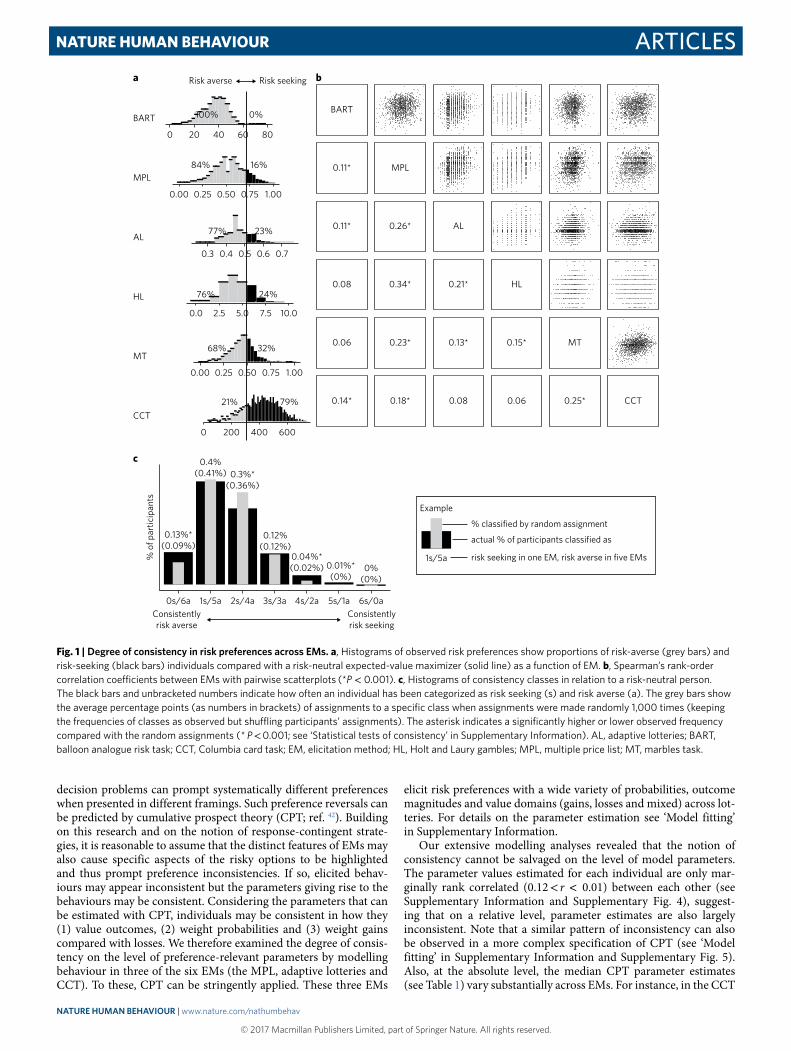
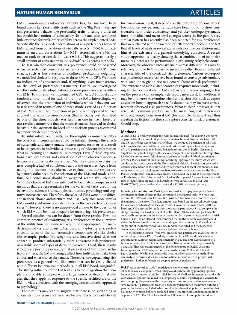
ResultsConsistency of risk preferences across EMs. At the outset, we categorized each individual’s behaviour relative to the baseline of expected value maximization (that is, the simplest normative model, which does not require any transformation of probabilities and outcomes and assumes risk neutrality). Using this baseline, we next compared individuals’ preferences across EMs. Figure 1a shows the distributions of individuals’ risk preferences (the proportion of choices for the riskier over the safer option) across all six EMs. The figure suggests that there are large differences in risk preferences across EMs. For instance, the proportion of individuals categorized as risk seekers ranged from 0 (in the BART) to 79% (in the CCT). Figure 1c shows how often a person was categorized as risk seeking or risk averse across the EMs. Only 13% of participants displayed the same risk preferences across all six EMs. A larger proportion of 53% of participants showed the same risk preferences in at least five of the six EMs. However, these observed proportions need to be considered in the context of the base rates of risk aversion and risk seeking in the different EMs before they can be interpreted as indicators of consistency. By repeatedly shuffling the assignments of participants within EMs 1,000 times and counting how often the shuffled participants showed identical risk preferences, estimations of the proportions due to pure base rate effects were calculated (see also ‘Statistical tests of consistency’ in Supplementary Information). The base-rate proportions (depicted in Fig.  1c in grey within the observed proportions in black bars) are by and large comparable to the observed proportions, suggesting that the observed consis-tency in assignments is primarily a consequence of base-rate effects. In sum, these results suggest that the six behavioural EMs elic-ited largely diverging preferences on an absolute level; the degree of overlap between the methods was barely higher than would be expected by chance.

Notwithstanding these inconsistencies, it could be that a per-son’s relative rank compared with others is constant across the EMs. For illustration, a score in a diagnostic screening test is infor-mative only relative to a norm distribution. By analogy, a person who is measured to be among the most risk-loving on one EM may also be measured to be one of the dare-devils on another EM. Consistent with this possibility, people’s rank orders on the differ-ent EMs were positively correlated between all EMs (Fig. 1b). Yet, the magnitudes of the correlations varied greatly, from insignificant

correlations close to zero (minimum Spearman’s rank-order cor-relations, r = 0.06) to moderate correlation coefficients (maximum Spearman’s rank-order correlations, r = 0.34). Thus, even if it is pos-sible to predict relative risk preferences assessed with EM A through behaviour measured with EM B, this extrapolation works only for some and not all behaviour-based EMs. In summary, the results show substantial across-method inconsistency in absolute risk pref-erences and little or moderate consistency in the relative ordering of individuals across methods.

Origins of people’s inconsistent risk preference measures. Some authors have suggested that inconsistency may be due to context-dependent risk preferences (for example, ref. 10), suggesting that people’s risk preferences pertaining to, for example, investment options might differ systematically from those pertaining to medi-cal options35. However, inconsistencies also emerged when similar EMs were applied in identical contextual frames and the choice architecture differed solely with respect to design features such as assortment, the order of choice sets14 or the magnitudes of the outcomes and probabilities12,14,15. To rule out this possibility in our study, we implemented EMs without explicit contextual frames.

Others have attributed inconsistent preferences to interactions of people’s cognitive ability and task complexity8,36; specifically, it has been suggested that differences in cognitive skills can affect people’s ability to reveal their true preferences in a given behavioural task to different degrees9. We tested whether individual differences in participants’ statistical numeracy—a construct that is strongly cor-related with cognitive ability37 but focuses on the comprehension of the operations of probabilistic and statistical computation—may have led to the apparent inconsistent risk preference measures. However, our analyses show that the observed inconsistencies were not significantly influenced by this factor (see ‘Inconsistency due to statistical numeracy’ in Supplementary Information).

Other sources that may attenuate consistency could be imposed by task-dependent and -independent measurement errors. Recently, Crosetto and Filippin21 examined the influence of task-specific measurement errors and showed in simulations that part of the observed across-task heterogeneity can be explained by task-specific measurement errors induced by the mere mechanics of the tasks at hand. Again, we found that after correcting for task-dependent and -independent measurement errors (see ‘Inconsistency due to measurement errors’ in  Supplementary Information) the overall picture remained by and large unchanged.

A final factor that could partially account for the observed inconsistent risk preferences is variability in how distinctly risk is expressed. The overall pattern of correlations indicates somewhat smaller consistency between the BART and the other EMs, com-pared with other tests. This could be explained by the fact that the BART involves decisions in which the underlying probabilities must be learned by the decision-maker. To disentangle the process of learning from risk preference in the BART, we modelled observed behaviour with the Bayesian sequential risk taking model38 (see ‘BSR model’ in Supplementary Information), but found qualitatively unchanged correlations when considering ‘learning-corrected’ risk preferences. Therefore, in summary, we conclude that these possi-ble explanations can only partially account for the widely observed inconsistent risk preferences.

A more general explanation has been discussed in a classic instance of inconsistent behaviour—the preference-reversal phe-nomenon39. Systematic reversals emerge as a function of the response mode (for example, binary choice, valuation and matching) through which people express their preference for otherwise equivalent lot-tery options. Different response modes, so the explanation goes, render distinct properties of options (for example, the magnitude of outcomes or probabilities) more prominent and consequently trig-ger distinct choice strategies7,40,41. Similarly, normatively identical

NATuRe HumAN BeHAviouR | www.nature.com/nathumbehav

© 2017 Macmillan Publishers Limited, part of Springer Nature. All rights reserved. © 2017 Macmillan Publishers Limited, part of Springer Nature. All rights reserved.

ArticlesNATurE HuMAN BEHAvIOur

decision problems can prompt systematically different preferences when presented in different framings. Such preference reversals can be predicted by cumulative prospect theory (CPT; ref. 42). Building on this research and on the notion of response-contingent strate-gies, it is reasonable to assume that the distinct features of EMs may also cause specific aspects of the risky options to be highlighted and thus prompt preference inconsistencies. If so, elicited behav-iours may appear inconsistent but the parameters giving rise to the behaviours may be consistent. Considering the parameters that can be estimated with CPT, individuals may be consistent in how they (1) value outcomes, (2) weight probabilities and (3) weight gains compared with losses. We therefore examined the degree of consis-tency on the level of preference-relevant parameters by modelling behaviour in three of the six EMs (the MPL, adaptive lotteries and CCT). To these, CPT can be stringently applied. These three EMs

elicit risk preferences with a wide variety of probabilities, outcome magnitudes and value domains (gains, losses and mixed) across lot-teries. For details on the parameter estimation see ‘Model fitting’ in Supplementary Information.

Our extensive modelling analyses revealed that the notion of consistency cannot be salvaged on the level of model parameters. The parameter values estimated for each individual are only mar-ginally rank correlated (0.12 < r < 0.01) between each other (see Supplementary Information and Supplementary Fig.  4), suggest-ing that on a relative level, parameter estimates are also largely inconsistent. Note that a similar pattern of inconsistency can also be observed in a more complex specification of CPT (see ‘Model fitting’ in Supplementary Information and Supplementary Fig. 5). Also, at the absolute level, the median CPT parameter estimates (see Table 1) vary substantially across EMs. For instance, in the CCT

0.13%*(0.09%)

0.4%(0.41%) 0.3%*

(0.36%)

0.12%(0.12%)

0.04%*(0.02%) 0.01%*

(0%)0%

(0%)

0s/6a 1s/5a 2s/4a 3s/3a 4s/2a 5s/1a 6s/0a

% o

f par

ticip

ants

BART

0.11* MPL

0.11* 0.26* AL

0.08 0.34* 0.21* HL

0.06 0.23* 0.13* 0.15* MT

0.14* 0.18* 0.08 0.06 0.25* CCT

100% 0%

0 20 40 60 80

84% 16%

0.00 0.25 0.50 0.75 1.00

77% 23%

0.3 0.4 0.5 0.6 0.7

76% 24%

0.0 2.5 5.0 7.5 10.0

68% 32%

0.00 0.25 0.50 0.75 1.00

21% 79%

0 200 400 600

BART

MPL

AL

HL

MT

CCT

Consistentlyrisk seeking

Consistentlyrisk averse

Risk seekingRisk averse

1s/5a

% classified by random assignment

actual % of participants classified as

risk seeking in one EM, risk averse in five EMs

Example

a b

c

Fig. 1 | Degree of consistency in risk preferences across ems. a, Histograms of observed risk preferences show proportions of risk-averse (grey bars) and risk-seeking (black bars) individuals compared with a risk-neutral expected-value maximizer (solid line) as a function of EM. b, Spearman’s rank-order correlation coefficients between EMs with pairwise scatterplots (*P < 0.001). c, Histograms of consistency classes in relation to a risk-neutral person. The black bars and unbracketed numbers indicate how often an individual has been categorized as risk seeking (s) and risk averse (a). The grey bars show the average percentage points (as numbers in brackets) of assignments to a specific class when assignments were made randomly 1,000 times (keeping the frequencies of classes as observed but shuffling participants’ assignments). The asterisk indicates a significantly higher or lower observed frequency compared with the random assignments (* P <  0.001; see ‘Statistical tests of consistency’ in Supplementary Information). AL, adaptive lotteries; BART, balloon analogue risk task; CCT, Columbia card task; EM, elicitation method; HL, Holt and Laury gambles; MPL, multiple price list; MT, marbles task.

NATuRe HumAN BeHAviouR | www.nature.com/nathumbehav

© 2017 Macmillan Publishers Limited, part of Springer Nature. All rights reserved. © 2017 Macmillan Publishers Limited, part of Springer Nature. All rights reserved.

Articles NATurE HuMAN BEHAvIOur

the typical participant (that is, described by median parameter esti-mates) is not loss averse but gain seeking (λ = 0.43) and sensitive to differences in the magnitudes of outcomes (α = 0.10). This ‘profile’ explains why many decision-makers emerged as more risk seeking in the CCT relative to the adaptive lottery and MPL methods. In the adaptive lotteries and MPL, however, the median CPT type exhib-its loss aversion (λ = 1.36 and 1.64, respectively) and is much more sensitive to differences in outcome magnitudes (α = 0.62 and 0.86, respectively).

One way consistency might be curtailed in these preference-relevant parameters is if distinct decision processes are used across different EMs. Most previous studies on method-dependent incon-sistency have implicitly assumed that all participants made deci-sions in accordance with EUT8,9,11–13,15,18; that is, they maximized the expected utility of their choices. However, numerous studies have demonstrated that individuals’ risk preferences often deviate from EUT and that CPT is often the best model for fitting aggre-gate choices even if some people are not best described by EUT and even though there may not be a single best model for fitting individual choices34,43,44.

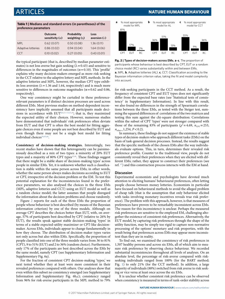
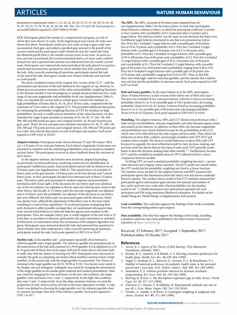
Consistency of decision-making strategies. Interestingly, two recent studies have shown that this heterogeneity can be parsimo-niously described as a mix of two types: a minority of 20% EUT types and a majority of 80% CPT types45,46. These findings suggest that there might be a stable share of ‘decision-making types’ across people in similar EMs. Yet, it is unknown whether such a classifica-tion is stable within the same person across EMs; in other words, whether the same person always makes decisions according to EUT or CPT, irrespective of the decision problem or the EM. To test this potential explanation for the inconsistencies found in the prefer-ence parameters, we also analysed the choices in the three EMs (MPL, adaptive lotteries and CCT) using an EUT model as well as a random choice model; the latter assumes that people disregard the information about the decision problems and choose randomly.

Figure  2 reports for each of the three EMs the proportion of people whose behaviour is best described (by means of the Bayesian information criterion) by one of the three models. Although on average CPT describes the choices better than EUT, with, on aver-age, 57% of participants best described by CPT (relative to 26% by EUT), the results speak against stable decision-making ‘types’ in terms of a stable expected-utility maximizer or CPT-like decision-maker. Across EMs, individuals appear to change fundamentally in how they choose. The distribution of decision-maker types varies not only across but also within EMs. Specifically, the proportion of people classified into one of the three models varies from 36 to 81% (CPT), 9 to 51% (EUT) and 2 to 36% (random choice). Furthermore, only 17% of the participants are best described across the EMs by the same model, namely CPT (see Supplementary Information and Supplementary Fig. 6a).

For the fraction of consistent CPT decision-making ‘types,’ we next tested whether they at least were more consistent in their revealed preferences compared with others. Our analyses show that even within this subset no consistency emerged (see Supplementary Information and Supplementary Fig.  6b,c); consistency ranged from 96% for risk-averse participants in the MPL method to 79%

for risk-seeking participants in the CCT method. As a result, the frequency of consistent CPT and EUT types does not significantly differ from the expected base rates (see ‘Statistical tests of consis-tency’ in  Supplementary Information). In line with this result, we also found no differences in the strength of Spearman’s correla-tions between the three EMs, as tested with the Steiger test, sum-ming the squared differences of  correlations of the two matrices and testing this sum against the chi-square distribution: Correlations within the subset of CPT ‘types’ were not stronger compared with those of the remaining 83% of participants (χ2 = 4.69, nCPT = 253, nother = 1,254, P < 0.2).

In summary, these findings do not support the existence of stable types of decision-makers who approach different tasks (EMs) on the basis of task-general decision processes. Instead, the results suggest that the specific methods of the chosen EMs alter the way individu-als evaluate options. This, in turn, determines their revealed risk preference profile. Counter to the traditional view, people do not consistently reveal their preferences when they are elicited with dif-ferent EMs; rather, they appear to construct their preferences (see ref. 47) and this construction process interacts with the EM at hand.

DiscussionExperimental economists and psychologists have devoted much attention to eliciting humans’ behavioural preferences, often letting people choose between money lotteries. Economists in particular have focused on behavioural methods to avoid the alleged problem of cheap talk (that is  the assumption that only behaviour elicited with tasks involving monetary incentives reveals true risk prefer-ence). The problem with this approach, however, is that measures of preferences have proven to be remarkably inconsistent across EMs. The reason for this inconsistency is unclear. Perhaps the measured risk preferences are sensitive to the employed EM, challenging alto-gether the existence of consistent risk preferences. Alternatively, the EUT model, by capturing risk preferences through the shape of the utility function, may be simply too rigid to capture non-normative processing of the options’ monetary and risk properties, with the result being that preferences across EMs may appear more inconsis-tent than they are in reality.

To find out, we examined the consistency of risk preferences in 1,507 healthy persons and across six EMs, all of which aim to mea-sure risk preference by observing choice behaviour. We recorded substantial inconsistencies throughout all levels of analyses. On an absolute level, the percentage of risk-averse compared with risk-seeking individuals ranged from 100% (for the BART method; Fig.  1) to only 21% (for the CCT method). In addition, a large majority of individuals (88%) switched from risk averse to risk seek-ing or vice versa at least once across the six EMs.

It is unclear whether consistent risk preference can be observed when consistency is measured in terms of rank-order stability across

Table 1 | medians and standard errors (in parentheses) of the preference parameters

outcome sensitivity (α )

Probability weighting (η )

Loss aversion (λ )

MPL 0.62 (0.07) 0.50 (0.08) 1.36 (0.11)

Adaptive lotteries 0.86 (0.02) 0.94 (0.04) 1.64 (0.06)

CCT 0.10 (0.02) 0.27 (0.05) 0.43 (0.01)

a b c

81%

17%2%

36%51%

13%

55%

9%

36%

% most appropriatemodel for MPL

% most appropriatemodel for AL

% most appropriatemodel for CCT

EUT RCCPT EUT RCCPT EUT RCCPT

Fig. 2 | Types of decision-makers across ems. a–c, The proportion of participants whose behaviour is best described by CPT, EUT or a random choice model (RC) varies substantially within and between EMs. a, MPL. b, Adaptive lotteries (AL). c, CCT. Classification according to the Bayesian information criterion value, taking the fit and model complexity into account.

NATuRe HumAN BeHAviouR | www.nature.com/nathumbehav

© 2017 Macmillan Publishers Limited, part of Springer Nature. All rights reserved. © 2017 Macmillan Publishers Limited, part of Springer Nature. All rights reserved.

ArticlesNATurE HuMAN BEHAvIOur

EMs. Considerable rank-order stability has, for instance, been found across key personality traits such as the ‘Big Five’48. Perhaps risk preference behaves like personality traits, offering a different but established notion of consistency. In our analyses, we found little evidence for rank-order stability across the implemented EMs. Specifically, the rank-order correlations of risk preferences between EMs ranged from correlations of virtually zero (r = 0.06) to a maxi-mum of medium correlations (r = 0.34). Across all the EMs, the median rank-order correlation was r = 0.11. This suggests merely a small amount of consistency in individuals’ ranks across methods.

To test whether consistent risk preference could be observed when we redefined consistency in terms of important CPT con-structs, such as loss aversion or nonlinear probability weighting, we modelled choices in response to three EMs with CPT. We found no indication of consistency and, if anything, even inconsistency on the level of preference parameters. Finally, we investigated whether individuals adopt distinct decision processes across differ-ent EMs. To this end, we implemented CPT, an EUT model and a random choice model for each of the three EMs. Interestingly, we observed that the proportion of individuals whose behaviour was best described in terms of one of three models varied as a function of EM. Moreover, the proportion of people who appeared to have adopted the same decision process (that is, being best described by one of the three models) was less than one in five. Therefore, our results demonstrate that the inconsistencies observed in choice behaviour also occur on the level of the decision process as captured by important decision models.

To substantiate our results, we thoroughly examined whether the observed inconsistencies could be inflated through the effects of systematic and unsystematic measurement error or as a result of heterogeneity in individuals’ processing of relevant information (that is, learning and statistical numeracy). Even if these explana-tions have some merit and even if some of the observed inconsis-tencies are idiosyncratic for some EMs, they cannot explain the near-complete lack of consistency across the measures. Apart from taking into account these alternative explanations, our results are, by nature, influenced by the selection of the EMs and models and, thus, our conclusions should be weighted within this selection. With the choice of EMs, we intended to facilitate a comparison of methods that are representative for the variety of tasks used in the behavioural sciences (for example, economics, psychology and cog-nitive neuroscience). Therefore, the selected EMs were quite differ-ent in their choice architectures and it is likely that more similar EMs would yield more consistency across the risk preference mea-sures49. However, there is no unequivocal answer to the question of which EM would be most adequate for measuring risk preferences.

Several conclusions can be drawn from these results. First, the common practice of quantifying risk preferences by the curvature of the utility function alone is likely to be inappropriate for many decision-makers and many EMs. Second, capturing risk prefer-ences in terms of the non-normative components of risky choice (for example, probability weighting and loss aversion) does not appear to produce substantially more consistent risk preferences or a stable share of types of decision-makers45. Third, these results strongly support the possibility that properties of the choice archi-tecture—here, the EMs—strongly affect how individuals make their choice and what choice they make. Therefore, conceptualizing risk preference as a general trait-like entity that can be easily elicited with different behavioural methods is, in all likelihood, misguided. The strong influence of the EM leads us to the suggestion that peo-ple are probably equipped with a large variety of decision strate-gies that they apply in response to the specific architecture of the EM—a view consistent with the emerging constructionist approach to psychology50.

These results may lead to suggest that there is no such thing as a consistent preference for risk. We believe this is too early to call

for two reasons. First, it depends on the definition of consistency. For instance, key personality traits have been found to show con-siderable rank-order consistency and yet they undergo systematic intra-individual and mean-level changes across the lifespan. A very similar pattern has recently also been reported for risk preferences that were elicited with the method of self-reports51. Second, the fact that all levels of analysis reveal exclusively positive correlations may hint at the existence of a general underlying construct. A recent study supports this idea by showing that a combination of many risk measures increases the performance in explaining risky behaviour20. Moreover, the observed inconsistencies across different EMs may be relatively unique to this class of measures rather than an inherent characteristic of the construct risk preference. Various self-report risk preference measures have been found to converge substantially with each other, giving rise to a general factor of risk preference52. The existence of such a latent construct requires more work, includ-ing further exploration of EMs whose architecture impinges less on the process (for example, self-report measures). In addition, it may be of interest to examine whether decision aids, such as expert advice on how to approach specific decisions, may increase consis-tency in observed risk preferences. What is clear, however, is that scientists’ common practice, namely, measuring risk preferences with one simple behavioural EM (for example, lotteries) and thus creating the fiction that they can capture consistent risk preferences, should stop.

methodsA total of 1,512 healthy participants without neurological (for example, epilepsy) or psychiatric (for example, depression or schizophrenia) disorders between 20 and 36 years of age were recruited. Of these, we excluded 5 participants who did not complete 4 or more of the behavioural tasks, resulting in a total sample size of 1,507 participants (746 in Basel, Switzerland, and 761 in Berlin, Germany). Supplementary Table 4 reports the socio-demographic information. The respective local ethics committees (Ethikkommission beider Basel and Ethikkommission des Max-Planck-Institut für Bildungsforschung) approved the study, which was conducted in accordance with the Declaration of Helsinki. Participants received a detailed explanation of the study and written informed consent was obtained. The study consisted of a day-long session in one of two laboratories—one at the Max Planck Institute for Human Development, Berlin, and the other at the Department of Psychology at the University of Basel. All of the reported P values from statistical tests of significance are two-sided. Analyses were conducted in MATLAB (8.6.0.267246) (www.mathworks.com) and R (3.3.0) (www.r-project.org).

Monetary incentivization. Participants received a fixed payment plus a bonus contingent on their choices in the incentivized behavioural tasks. We took into account the different wage levels at the Swiss and German study centres to match the monetary incentives. The fixed amount was based on the typical hourly wage for research assistants at the local universities, namely, 15 Swiss francs (CHF) in Basel and € 10 euros in Berlin. It took most participants about 8 h to complete the study, resulting in a fixed payment of CHF 120 or € 80. In addition, participants collected bonus points in the incentivized tasks. Participants started with an initial bonus of CHF 15 or € 10 and were informed that in the extreme case, they could either double or lose this amount, depending on their choices. At the end of the study, one of the incentivized tasks was randomly selected and the respective outcome was either added to or subtracted from the initial bonus.

In the morning session (from 9:00 am to noon), participants made choices in seven risk-preference EMs. The design features of the EMs and their schematic appearance is summarized in Supplementary Fig 1. The EMs were assessed in a time of no more than 2.5 h, interleaved with 10 min breaks after approximately 1 and 2 h. They were administered in the following order: BART, decisions from experience, CCT, adaptive lotteries, marbles task, MPL and Holt and Laury gambles. We did not include the decisions from experience method53 in our analysis because it does not aim for a direct measurement of people’s risk preferences. Rather, it focuses on people’s extent of exploration.

BART. As in an earlier study54, participants were sequentially presented with 30 balloons on a computer screen. They could earn points by pumping up each balloon (with mouse clicks). Each click inflated the balloon incrementally and with each click one point was added to a temporary account. If participants decided to stop pumping, the points on the temporary account were moved to a permanent save account. If participants reached a randomly determined maximum number of pumps, the balloon exploded, which resulted in a loss of all points accrued for that balloon. On average, balloons exploded after 64 pumps with a maximum number of pumps of 128. The 30 balloons had the following explosion points (and were

NATuRe HumAN BeHAviouR | www.nature.com/nathumbehav

© 2017 Macmillan Publishers Limited, part of Springer Nature. All rights reserved. © 2017 Macmillan Publishers Limited, part of Springer Nature. All rights reserved.

Articles NATurE HuMAN BEHAvIOur

presented in randomized order): 1, 13, 18, 22, 28, 30, 33, 37, 47, 49, 50, 55, 56, 58, 61, 67, 70, 72, 73, 78, 79, 81, 91, 95, 98, 100, 106, 110, 115 and 128. Each pump in a successful balloon equated to CHF 0.008 or € 0.005.

CCT. Participants played 84 rounds of a computerized card game, in each of which they were shown 32 cards. At the beginning of each round, all cards were shown face down. Participants could turn over cards as long as gain cards were encountered. Each gain card added a specified gain amount to the payoff of the current round and the participant could voluntarily stop the round and claim the obtained payoff (that is, the round’s current score) at any time. As soon as a loss card was encountered, the round terminated; that is, no more cards could be turned over and a specified loss amount was subtracted from the round’s current score. Participants were interactively instructed about the task, played two practice rounds and answered four questions to check whether they fully understood the task. After correctly answering all questions, participants started the task. At the end of the task, three game rounds were chosen randomly and summed to a total payoff.

We used a modified version of the original ‘hot’ version of the CCT55, with the presentation and structure of the task identical to the original set-up. However, to obtain precise parameter estimates of the value and probability weighting functions in the decision models it was advantageous to sample decision behaviour for a wide range of outcome magnitudes and probability levels (see Supplementary Table 5). Thus, we extended the current task to include game rounds with medium-to-high probabilities of losses; that is, 10, 16, 20 or 28 loss cards, compared with the maximum of 3 loss cards in the original CCT. This provided additional data points for estimating the probability weighting function of CPT for medium-to-high probabilities. Second, to enable precise estimation of the value functions, we also extended the range of gain amounts to amounts of 10, 20, 50, 75, 100, 150, 200, 300, 400 and 600 points per gain card (original version: 10, 20 and 30 points per gain card). Third, the loss amounts were similarly extended to 25, 50, 75, 100, 150, 250, 500 and 750 points per loss card (original version: 250, 500 and 750 points per loss card). Note that the placement of cards of all types was random. Each point equated to CHF 0.022 or € 0.015.

Adaptive lotteries. Participants made choices between 75 and 100 (mean = 80.6, s.d. = 2.9) pairs of two-outcome lotteries. Each lottery’s magnitude of outcomes was presented as numbers and the underlying probabilities were presented as numbers and pie charts. The participants received no direct feedback about the outcome of their choice.

In the adaptive lotteries, the lotteries were iteratively adapted depending on previously revealed preferences, rendering a more precise identification of participants’ indifference points. Each participant started with an identical set of 25 lottery pairs (see Supplementary Table 6). This initial lottery set included 10 lottery pairs in the gain domain, 10 lottery pairs in the loss domain and 5 mixed lottery pairs. At first, participants decided twice between each of these 25 lottery pairs. The lottery pairs were presented in random sequence and presentation orientation (left versus right). If the decisions for one lottery pair were identical, one of the two lotteries was adjusted so that its expected value became closer to the other lottery. Specifically, in 15 lottery pairs the outcome magnitude was adjusted and in 10 lottery pairs the probability was adjusted. If the decisions in one lottery pair were different, the lottery pair was presented again and the decision, which was chosen twice, affected the adjustment of the lottery pair in the next round (resulting in a total of four repetitions). To avoid participants strategizing their early decisions to affect possible earnings later, we randomized subsequent steps from several initial lotteries to make the lotteries appear more random to the participants. Thus, for example, lottery pair A could reappear in the next trial or 25 trials later, or anywhere in between, presented in the same orientation or switched. Furthermore, no information about the mechanism of the adaptive algorithm was given. Participants were instructed about the task and answered four questions to check whether they fully understood it. After correctly answering all questions, participants started the task. Each point equated to CHF 0.10 or € 0.07.

Marbles task. In the marbles task56, participants repeatedly chose between a reference gamble and a target gamble. The reference gamble was presented only in the instructions of the task and consisted of a 50/50 gamble. It was displayed as a 10 by 10 grid with 50 black dots in the upper half and 50 white dots in the lower half, to make clear that the chance of winning was 50%. Participants were instructed to consider the grids as containing win tickets (black marbles) and loss tickets (white marbles). In the actual task, only the target gamble was presented. The chance of winning in the target gamble was 45/55, 50/50 or 55/45. Two factors were varied in the design: risk and ambiguity. Ambiguity was varied by changing the presentation of the target gambles in the marble grids (ordered and random presentation). Risk was varied by changing the wins and losses. In the low-risk condition, the target gambles’ wins and losses were 1 and –1, respectively. In the high-risk condition, they were 3 and –3, respectively. As in the other monetary lotteries, we used the proportion of risky choices across all trials as the main dependent variable. A risky choice was defined as choosing the target gamble over the reference gamble when its variance was larger than that of the reference gamble. Each point equated to CHF 1 or € 0.7.

The MPL. The MPL consisted of 56 lottery pairs adapted from ref. 57 (see Supplementary Table 7 for the lottery pairs). In each trial, participants chose between a reference lottery, in which the participant could win 15 points or lose 5 points with a probability of 0.5 (expected value = 5 points) and a target lottery. The reference lottery was the same in each decision, but there were 56 different target lotteries structured in sets that were presented as 6 price lists. Price list 1 included 7 target lotteries with a possible gain of 60 points, loss of 10 to 70 points and a probability of 0.5. Price list 2 included 5 target lotteries with a possible gain of 30 points, loss of 0.1 to 40 points and a probability of 0.5. Price list 3 included 16 target lotteries with a possible gain of 50 to 200 points, loss of 60 points and a probability of 0.5. Price list 4 included 11 target lotteries with a possible gain of 20 to 120 points, loss of 30 points and a probability of 0.5. Price list 5 included 11 target lotteries with a possible gain of 60 points, loss of 60 points and a probability ranging from 0.46 to 0.91. Price list 6 included 6 target lotteries with a possible gain of 30 points, loss of 30 points and a probability ranging from 0.42 to 0.91. Thus, in this EM, there were both high- and low-outcome gambles, and the amount that could be won and lost and the probability of outcomes varied. Each point equated to CHF 0.075 or € 0.05.

Holt and Laury gambles. In the same fashion as in the MPL, participants chose 10 times between a scaled version of the lottery sets of Holt and Laury28. The price list included 10 two-outcome lotteries. Lotteries A had an increasing probability (from 0.1 to 1) of a possible gain of 192.5 points and a decreasing probability (from 0.9 to 0) of 5 points. Lotteries B had an increasing probability (from 0.1 to 1) of a possible gain of 80 points and a decreasing probability (from 0.9 to 0) of 70 points. Each point equated to CHF 0.075 or € 0.05.

Modelling. The adaptive lotteries, MPL and CCT elicited risk preferences with a wide variety of probabilities, outcome magnitudes and value domains (gains, losses and mixed) across lotteries. In addition, in these EMs, the outcome magnitudes and probabilities were clearly defined (except for the probabilities in the CCT, which were to be inferred from the ratio of gain and loss cards). Thus, observed behaviour in these EMs could be convincingly modelled with CPT, EUT and random choice models. We chose to model behaviour in these EMs with CPT because it is arguably the most influential model in risky decision-making, and previous work has shown that for the types of tasks used, CPT generally works better to describe decision-making than other models58,59. Furthermore, because EUT could be modelled as simplification of CPT it offered itself for a direct comparison between models.

In fitting CPT, we used a standard probability weighting function60, a power value function and a logistic choice function. The EUT model was nested within the CPT model but the probability weighting was fixed to a linear function. The random choice models for the adaptive lotteries and MPT assumed that participants ignore the information about the lottery sets and choose randomly between options. The random choice model of the CCT similarly assumed that participants ignore information (gain amount, loss amount and number of loss cards) and turn over cards with a fixed probability (see the baseline model in ref. 38). Model parameters were determined separately for each participant and EM using maximum likelihood estimation. For details on the model fitting see ‘Model fitting’ in Supplementary Information.

Code availability. The code that supports the findings of this study is available from the corresponding author upon request.

Data availability. The data that support the findings of this study, including a detailed codebook, have been published in the Open Science Framework repository at https://osf.io/rce7g.

Received: 23 February 2017; Accepted: 1 September 2017; Published: xx xx xxxx

References 1. Arrow, K. J. Aspects of the Theory of Risk-Bearing. (Yrjö Jahnssonin

Foundation, Helsinki, 1965). 2. Booske, B. C., Sainfort, F. & Hundt, A. S. Eliciting consumer preferences for

health plans. Health Serv. Res. 34, 839–854 (1999). 3. Saigal, S., Stoskopf, B. L., Burrows, E., Streiner, D. L. & Rosenbaum, P. L.

Stability of maternal preferences for pediatric health states in the perinatal period and 1 year later. Arch. Pediatr. Adolesc. Med. 157, 261–269 (2003).

4. Samuelson, P. A. Lifetime portfolio selection by dynamic stochastic programming. Rev. Econ. Stat. 51, 239–246 (1969).

5. Hertwig, R. & Erev, I. The description–experience gap in risky choice. Trends Cogn. Sci. 13, 517–523 (2009).

6. Charness, G., Gneezy, U. & Halladay, B. Experimental methods: pay one or pay all. J. Econ. Behav. Organ. 131, 141–150 (2016).

7. Tversky, A., Sattath, S. & Slovic, P. Contingent weighting in judgment and choice. Psychol. Rev. 95, 371–384 (1988).

NATuRe HumAN BeHAviouR | www.nature.com/nathumbehav

© 2017 Macmillan Publishers Limited, part of Springer Nature. All rights reserved. © 2017 Macmillan Publishers Limited, part of Springer Nature. All rights reserved.

ArticlesNATurE HuMAN BEHAvIOur

8. Anderson, L. R. & Mellor, J. M. Are risk preferences stable? Comparing an experimental measure with a validated survey-based measure. J. Risk Uncertain. 39, 137–160 (2009).

9. Dave, C., Eckel, C. C., Johnson, C. A. & Rojas, C. Eliciting risk preferences: when is simple better? J. Risk Uncertain. 41, 219–243 (2010).

10. Reynaud, A. & Couture, S. Stability of risk preference measures: results from a field experiment on French farmers. Theory Decis. 73, 203–221 (2012).

11. Dulleck, U., Fooken, J. & Fell, J. Within-subject intra- and inter-method consistency of two experimental risk attitude elicitation methods. German Econ. Rev. 16, 104–121 (2013).

12. Deck, C., Lee, J., Reyes, J. A. & Rosen, C. C. A failed attempt to explain within subject variation in risk taking behavior using domain specific risk attitudes. J. Econ. Behav. Organ. 87, 1–24 (2013).

13. Szrek, H., Chao, L. W., Ramlagan, S. & Peltzer, K. Predicting (un)healthy behavior: a comparison of risk-taking propensity measures. Judgm. Decis. Mak. 7, 716–727 (2012).

14. Bruner, D. M. Changing the probability versus changing the reward. Exp. Econ. 12, 367–385 (2009).

15. Ihli, H. J., Chiputwa, B. & Musshoff, O. Do changing probabilities or payoffs in lottery-choice experiments affect risk preference outcomes? Evidence from rural Uganda. J. Agr. Resour. Econ. 41, 324–345 (2016).

16. Deck, C., Lee, J. & Reyes, J. Investing versus gambling: experimental evidence of multi-domain risk attitudes. Appl. Econ. Let. 21, 19–23 (2013).

17. Isaac, R. M. & James, D. Just who are you calling risk averse? J. Risk Uncertain. 20, 177–187 (2000).

18. Berg, J., Dickhaut, J. & McCabe, K. Risk preference instability across institutions: a dilemma. Proc. Natl Acad. Sci. USA 102, 4209–4214 (2005).

19. Harbaugh, W. T., Krause, K. & Vesterlund, L. The fourfold pattern of risk attitudes in choice and pricing tasks. Econ. J. 120, 595–611 (2010).

20. Menkhoff, L. & Sakha, S. Estimating risky behavior with multiple-item risk measures. J. Econ. Psychol. 59, 59–86 (2017).

21. Crosetto, P. & Filippin, A. A theoretical and experimental appraisal of four risk elicitation methods. Exp. Econ. 19, 613–641 (2016).

22. He, P., Veronesi, M. & Engel, S. Consistency of Risk Preference Measures and the Role of Ambiguity: An Artefactual Field Experiment from China (WP 3, Working Paper Series, Department of Economics, Univ. Verona, 2016).

23. Loomes, G. & Pogrebna, G. Measuring individual risk attitudes when preferences are imprecise. Econ. J. 124, 569–593 (2014).

24. Nielsen, T., Keil, A. & Zeller, M. Assessing farmers’ risk preferences and their determinants in a marginal upland area of Vietnam: a comparison of multiple elicitation techniques. Agric. Econ. 44, 255–273 (2013).

25. Drichoutis, A. & Lusk, J. What can multiple price lists really tell us about risk preferences? J. Risk Uncertain. 53, 89–106 (2016).

26. Fausti, S. W. & Gillespie, J. M. A comparative analysis of risk preference elicitation procedures using mail survey results In Annual Meetings of the Western Agricultural Economics Association, Vancouver, Canada (Western Agricultural Economics Association, 2000).

27. Von Neumann, J. & Morgenstern, O. Theory of Games and Economic Behavior (Princeton Univ. Press, Princeton, NJ, 1947).

28. Holt, C. A. & Laury, S. K. Risk aversion and incentive effects. Am. Econ. Rev. 92, 1644–1655 (2002).

29. Lejuez, C. et al. Evaluation of a behavioral measure of risk taking: the Balloon Analogue Risk Task (BART). J. Exp. Psychol. Appl. 8, 75 (2002).

30. Hey, J. D. & Orme, C. Investigating generalizations of expected utility theory using experimental data. Econometrica 62, 1291–1326 (1994).

31. Figner, B., Mackinlay, R. J., Wilkening, F. & Weber, E. U. Affective and deliberative processes in risky choice: age differences in risk taking in the Columbia Card Task. J. Exp. Psychol. Learn. Mem. Cogn. 35, 709–730 (2009).

32. Dutilh, G. & Rieskamp, J. Comparing perceptual and preferential decision making. Psychon. Bull. Rev. 23, 723–737 (2015).

33. Markowitz, H. Portfolio selection. J. Finance 7, 77–91 (1952). 34. Starmer, C. Developments in non-expected utility theory: the hunt for a

descriptive theory of choice under risk. J. Econ. Lit. 38, 332–382 (2000). 35. Lejarraga, T., Pachur, T., Frey, R. & Hertwig, R. Decisions from experience:

from monetary to medical gambles. J. Behav. Decis. Mak. 29, 67–77 (2016). 36. Pachur, T., Mata, R. & Hertwig, R. Who dares, who errs? Disentangling

cognitive and motivational roots of age differences in decisions under risk. Psychol. Sci. 28, 504–518 (2017).

37. Cokely, E. T., Galesic, M., Schulz, E., Ghazal, S. & Garcia-Retamero, R. Measuring risk literacy: the Berlin numeracy test. J. Behav. Decis. Mak. 7, 25–47 (2012).

38. Wallsten, T. S., Pleskac, T. J. & Lejuez, C. Modeling behavior in a clinically diagnostic sequential risk-taking task. Psychol. Rev. 112, 862–880 (2005).

39. Lichtenstein, S. & Slovic, P. Reversals of preference between bids and choices in gambling decisions. J. Exp. Psychol. 89, 46–55 (1971).

40. Payne, J. W. Contingent decision behavior. Psychol. Bull. 92, 382–402 (1982). 41. Slovic, P. & Lichtenstein, S. Preference reversals: a broader perspective. Am.

Econ. Rev. 73, 596–605 (1983). 42. Tversky, A. & Kahneman, D. in Environmental Impact Assessment,

Technology Assessment, and Risk Analysis (eds Covello, V. T., Mumpower, J. L., Stallen, P. J. M. & Uppuluri, V. R. R.) 107–129 (Springer-Verlag, Berlin, Heidelberg, 1985).

43. Hey, J. D. & Orme, C. Investigating generalizations of expected utility theory using experimental data. Econometrica 62, 1291–1326 (1994).

44. Harless, D. W. & Camerer, C. F. The predictive utility of generalized expected utility theories. Econometrica 62, 1251–1289 (1994).

45. Bruhin, A., Fehr-Duda, H. & Epper, T. Risk and rationality: uncovering heterogeneity in probability distortion. Econometrica 78, 1375–1412 (2010).

46. Conte, A., Hey, J. D. & Moffatt, P. G. Mixture models of choice under risk. J. Econ. 162, 79–88 (2011).

47. Slovic, P. The construction of preference. Am. Psychol. 50, 364–371 (1995). 48. Ferguson, C. J. A meta-analysis of normal and disordered personality across

the life span. J. Pers. Soc. Psychol. 98, 659–667 (2010). 49. Vieider, F. M. et al. Common components of risk and uncertainty attitudes

across contexts and domains: evidence from 30 countries. J. Eur. Econ. Assoc. 13, 421–452 (2015).

50. Mesquita, B., Barrett, L. F. & Smith, E. R. The Mind in Context (Guilford Press, New York, 2010).

51. Josef, A. K. et al. Stability and change in risk-taking propensity across the adult life span. J. Pers. Soc. Psychol. 111, 430–450 (2016).

52. Frey, R., Pedroni, A., Mata, R., Rieskamp, J. & Hertwig, R. Risk preference shares the psychometric structure of major psychological traits. Sci. Adv. (in the press).

53. Hertwig, R., Barron, G., Weber, E. U. & Erev, I. Decisions from experience and the effect of rare events in risky choice. Psychol. Sci. 15, 534–539 (2004).

54. Lejuez, C. et al. Evaluation of a behavioral measure of risk taking: the balloon analogue risk task (BART). J. Exp. Psychol. Appl. 8, 75–84 (2002).

55. Figner, B., Mackinlay, R. J., Wilkening, F. & Weber, E. U. Affective and deliberative processes in risky choice: age differences in risk taking in the Columbia Card Task. J. Exp. Psychol. Learn. Mem. Cogn. 35, 709–730 (2009).

56. Dutilh, G. & Rieskamp, J. Comparing perceptual and preferential decision making. Psychon. Bull. Rev. 23, 723–737 (2015).

57. Von Helversen, B. & Rieskamp, J. Does the influence of stress on financial risk taking depend on the riskiness of the decision? In 35th Annual Conference of the Cognitive Science Soc. 1546–1551 (2013).

58. Rieskamp, J. The probabilistic nature of preferential choice. J. Exp. Psychol. Learn. Mem. Cogn. 34, 1446–1465 (2008).

59. Glöckner, A. & Pachur, T. Cognitive models of risky choice: parameter stability and predictive accuracy of prospect theory. Cognition 123, 21–32 (2012).

60. Prelec, D. The probability weighting function. Econometrica 66, 497–527 (1998).

AcknowledgementsThis paper benefited from many helpful comments from the members of the Center for Economic Psychology at the University of Basel. We thank S. Goss and L. Wiles for editing this manuscript. This work was supported by the Swiss National Science Foundation with a grant to J.R. and R.H. (CRSII1_136227). The funders had no role in study design, data collection and analysis, decision to publish or preparation of the manuscript.

Author contributionsA.P., R.F., A.B., G.D., R.H. and J.R. designed the research and wrote the paper. A.P. and R.F. performed the experimental studies. A.P., R.F. and A.B. analysed the data.

Competing interestsThe authors declare no competing interests.

Additional informationSupplementary information is available for this paper at doi:10.1038/s41562-017-0219-x.

Reprints and permissions information is available at www.nature.com/reprints.

Correspondence and requests for materials should be addressed to A.P.

Publisher’s note: Springer Nature remains neutral with regard to jurisdictional claims in published maps and institutional affiliations.

NATuRe HumAN BeHAviouR | www.nature.com/nathumbehav

1

nature research | life sciences reporting summ

aryJune 2017

Corresponding author(s): Andreas Pedroni

Initial submission Revised version Final submission

Life Sciences Reporting SummaryNature Research wishes to improve the reproducibility of the work that we publish. This form is intended for publication with all accepted life science papers and provides structure for consistency and transparency in reporting. Every life science submission will use this form; some list items might not apply to an individual manuscript, but all fields must be completed for clarity.

For further information on the points included in this form, see Reporting Life Sciences Research. For further information on Nature Research policies, including our data availability policy, see Authors & Referees and the Editorial Policy Checklist.

Experimental design1. Sample size

Describe how sample size was determined. The sample size was chosen to be able to robustly model individual differences in risk preferences in addition it was intended to facilitate genetic analyses (that are not reported in this manuscript but will possibly be combined with other samples).

2. Data exclusions

Describe any data exclusions. We excluded 5 participants who did not complete 4 or more of the behavioral tasks, resulting in a total sample size of 1,507 participants.

3. Replication

Describe whether the experimental findings were reliably reproduced.

No attempt to reproduce the findings was made.

4. Randomization

Describe how samples/organisms/participants were allocated into experimental groups.

The study does not involve experimental groups.

5. Blinding

Describe whether the investigators were blinded to group allocation during data collection and/or analysis.

There was no blinding of the investigators.

Note: all studies involving animals and/or human research participants must disclose whether blinding and randomization were used.

6. Statistical parameters For all figures and tables that use statistical methods, confirm that the following items are present in relevant figure legends (or in the Methods section if additional space is needed).

n/a Confirmed

The exact sample size (n) for each experimental group/condition, given as a discrete number and unit of measurement (animals, litters, cultures, etc.)

A description of how samples were collected, noting whether measurements were taken from distinct samples or whether the same sample was measured repeatedly

A statement indicating how many times each experiment was replicated

The statistical test(s) used and whether they are one- or two-sided (note: only common tests should be described solely by name; more complex techniques should be described in the Methods section)

A description of any assumptions or corrections, such as an adjustment for multiple comparisons

The test results (e.g. P values) given as exact values whenever possible and with confidence intervals noted

A clear description of statistics including central tendency (e.g. median, mean) and variation (e.g. standard deviation, interquartile range)

Clearly defined error bars

See the web collection on statistics for biologists for further resources and guidance.

2

nature research | life sciences reporting summ

aryJune 2017

SoftwarePolicy information about availability of computer code

7. Software

Describe the software used to analyze the data in this study.

We used Matlab, R and JAGS and indicate wherever we have used additional packages.

For manuscripts utilizing custom algorithms or software that are central to the paper but not yet described in the published literature, software must be made available to editors and reviewers upon request. We strongly encourage code deposition in a community repository (e.g. GitHub). Nature Methods guidance for providing algorithms and software for publication provides further information on this topic.

Materials and reagentsPolicy information about availability of materials

8. Materials availability

Indicate whether there are restrictions on availability of unique materials or if these materials are only available for distribution by a for-profit company.

Not applicable.

9. Antibodies

Describe the antibodies used and how they were validated for use in the system under study (i.e. assay and species).

Not applicable.

10. Eukaryotic cell linesa. State the source of each eukaryotic cell line used. Not applicable.

b. Describe the method of cell line authentication used. Not applicable.

c. Report whether the cell lines were tested for mycoplasma contamination.

Not applicable.

d. If any of the cell lines used are listed in the database of commonly misidentified cell lines maintained by ICLAC, provide a scientific rationale for their use.

Not applicable.

Animals and human research participantsPolicy information about studies involving animals; when reporting animal research, follow the ARRIVE guidelines

11. Description of research animalsProvide details on animals and/or animal-derived materials used in the study.

The study included human research participants.

Policy information about studies involving human research participants

12. Description of human research participantsDescribe the covariate-relevant population characteristics of the human research participants.

1,507 (748 in Basel, Switzerland, 762 in Berlin, Germany) healthy participants without neurological (e.g., epilepsy) or psychiatric (e.g., depression, schizophrenia) disorders between 20 and 36 years of age.