The Returns to the Federal Tax Creditsfor Higher Education*

George B. Bulman , Caroline M. Hoxby†† †††

August 2014

ABSTRACT

Three tax credits benefit households who pay tuition and fees for highereducation. The credits have been justified as an investment: generating moreeducated people and thus more earnings and externalities associated witheducation. The credits have also been justified purely as tax cuts to benefit themiddle class. In 2009, the generosity of and eligibility for the tax creditsexpanded enormously so that their 2011 cost was $25 billion. Using selected,de-identified data from the population of potential return filers, we show howthe credits are distributed across households with different incomes. Weestimate the causal effects of the federal tax credits using two empiricalstrategies (regression kink and simulated instruments) which we show to bestrong and very credibly valid for this application. The latter strategy exploitsthe massive expansion of the credits in 2009. We present causal estimates ofthe credits' effects on postsecondary attendance, the type of college attended,the resources experienced in college, tuition paid, and financial aid received. We discuss the implications of our findings for society's return on investmentand for the tax credits' budget neutrality over the long term (whether higherlifetime earnings generate sufficient taxes to recoup the tax expenditures). Weassess several explanations why the credits appear to have negligible causaleffects.

The opinions expressed in this paper are those of the authors alone and do not*

necessarily represent the views of the Internal Revenue Service or the U.S. TreasuryDepartment. This work is a component of a larger project examining the effects offederal tax and other expenditures that affect higher education. Selected, de-identifieddata were accessed through contract TIR-NO-12-P-00378 with the Statistics of Income(SOI) Division at the U.S. Internal Revenue Service. The authors gratefullyacknowledge the help of Barry W. Johnson of the Statistics of Income Division, InternalRevenue Service.

University of California Santa Cruz††

Stanford University and NBER†††

1

1 Introduction to the Tax Credits for Higher EducationSince 1997 the U.S. federal government has offered tax credits--the Hope TaxCredit (HTC) and Tax Credit for Lifelong Learning (TCLL)--to households whopay tuition and fees for higher education. In 2009, the enactment of theAmerican Opportunity Tax Credit (AOTC) made the postsecondary tax creditsmuch more generous. It also expanded eligibility for the credits to a largenumber of low-income and higher-income households that had previously beenineligible. The estimated fiscal cost of the tax credits is $23 billion for 2014. For comparison, the much better-known Pell Grant program, which providesgrants to low-income students, cost approximately $33 billion in the same year. All other federal programs that support higher education are smaller.

From 1997 to today, proponents have offered two main justifications forthe tax credits. The first is that tax credits will induce individuals to investmore in their own education, causing them to have improved earnings andother improved outcomes (some of which may occur through social mechanismssuch as educational spillovers or reduced dependency). The improvements willbe such that the tax credits ultimately pay for themselves--for the federalgovernment in particular or for society in general. Hereafter, we classifyarguments under this general heading as "return on investment" (ROI)arguments.

Some proponents of the tax credits have suggested, as a secondjustification, that they are simply a tax cut--more especially a "middle class taxcut." Although this justification has always been more controversial than theROI argument, it is safe to say that at least some proponents would judge thecredits to be successful if they could be shown to be an efficient means ofreducing taxes relative to other tax cuts with similar incidence.

In this paper, we show how the tax expenditures associated with the taxcredits are distributed among households. This evidence should help readersassess the credits' distributional consequences purely as tax cuts. Most of thestudy is, however, dedicated to assessing the ROI argument. It is logicallynecessary for this argument that the tax credits have a causal effect on someeducational outcome such as college attendance, the educational resourcesstudents experience, or the type of college students attend. Once one hasobtained causal effects on such outcomes, one can project their long-termconsequences by, for instance, by associating changes in college attendancewith changes in lifetime earnings.

The main challenge in this study is to identifying causal effects of the taxcredits. Our first approach relies on the phase-out of each tax credit. Eachphase-out creates two kinks in an otherwise linear relationship betweenhousehold income and the tax credit obtainable. These kinks allow us to useregression kink methods to estimate effects of the tax credits. These methodsare very suitable not only because they can produce highly credibly causalestimates but also because we estimate the kinks precisely using dense datafrom the population of potential tax returns. The limitation of the regressionkink estimates is that they inform us only about causal effects for households

2

in the vicinity of the phase-out range of income. If the effects on thesehouseholds is dissimilar from the effects on, say, low-income households, wehave learned only part of the story.

Therefore, we also use the method of simulated instruments to analyze theeffects of the tax credits. In particular, we look before and after the enactmentof the AOTC in 2009. This enactment effectively greatly increased thegenerosity of the tax credits and also extended credits to households that hadpreviously been ineligible. Thus, we have "before" and "after" periods and wehave households whose eligibility was changed ("treated") and whose eligibilitywas unchanged ("controls"): the ingredients of a classic difference-in-differences analysis. Because the changes in tax credits are complicated, weform simulated instruments that embody the policy-driven (and only the policy-driven) changes in the credits available to a household. Nevertheless, oneshould think of the simulated instruments analysis as logically analogous toa differences-in-differences analysis.

The advantage of the simulated instruments analysis is that we can assessthe effects of the tax credits on households of all income levels, not justhouseholds in the phase-out ranges. However, a disadvantage is that the 2008to 2009 period is hard to analyze because the financial crisis and recessionmight also have affected higher education. For instance, the method would beundermined by effects of the business cycle that differ for students withdifferent family incomes. Nevertheless, we are confident that our simulatedinstruments findings can dependably be interpreted as causal. Our confidenceis based on three facts. First, changes in the generosity of the tax credits werespread throughout the income distribution. There were low-income, middle-income, and high-income individuals who were "treated." Similarly, there werelow-, middle-, and high-income "controls" who experienced little or no changein the tax credits. Second, we can show that individuals who would be more orless affected by the enactment of the AOTC were on parallel trends, in termsof college outcomes, prior to the AOTC. Third, when applied to the relativelyhigh income individuals for whom we have regression kink results, thesimulated instruments method produces results that are essentially the same.

Having produced credible estimates of the causal effects of the tax creditson outcomes such as college attendance, we consider the implications for theROI argument. We conclude the paper by discussing explanations for theapparently negligible causal effects of the tax credits. We also discuss the taxcredits purely as tax cuts.

We benefit from several excellent, previous studies of the tax credits forhigher education. Crandall-Hollick (2012a, 2012b) concisely summarizes the provisions of the higher education tax credits and the legislative debatesurrounding them. Lederman's (1997) narrative about the lobbying for andpassage of the tax credits is highly informative about the announced intentionsof their proponents. Several previous studies have predicted the impact of thecredits or highlighted their peculiar features: Hoxby (1998), Davis (2002),Dynarski and Scott-Clayton (2006), Kane (1997), and Maag and Rohlay (2007).

3

Long (2004b) assesses the impact of the initial introduction of the credits. She uses the data from the National Postsecondary Student Aid Survey toshow their distributional consequences. She then uses differences-in-differences methods on the 1990 through 2000 October EnrollmentSupplements to the Current Population Survey to show that the introductionof the tax credits appears to have generated little or no increase inpostsecondary enrollment. Long classifies students based on their actualeligibility for the credit.

Like Long (2004b), Turner (2011) analyzes the initial enactment of the taxcredits. He relies on data from the 1996 and 2001 waves of the Survey ofIncome and Program Participation, and uses an approach that is essentiallydifferences-in-differences. However, he classifies students by their potentialeligibility for the credits. In other work, Turner (2012a, 2012b) investigateswhether the tax credits are offset by tuition increases and why many filers failto take the tax credit that would apparently benefit them most.

Relative to Long (2004b) and Turner (2011), we make severalimprovements. First, we use data from the population of potential tax returnfilers. These allow us to be fairly definitive about the distributionalconsequences of the credits. They also allow us to use the regression kinkmethod--a method that is not reliable with data that is less than very dense. (Unfortunately, certain key variables are not available before 1999 so we do notstudy the initial enactment of the credits.) Second, although we cannot studythe initial introduction of the tax credits, the enactment of the AOTC providesus with a much larger shock to tax expenditures than the initial introductionprovided. The fiscal cost of the credits rose by $12 billion between 2008 and2009 ($2014 dollars). The fiscal cost rose by only $4.9 billion when the creditswere initially introduced ($2014 dollars). The AOTC also affected householdsover a much wider range of incomes than the HTC and TCLL Third, our useof simulated instruments is a major improvement over both the Long andTurner methods. This point is a bit subtle but boils down to the fact that weobserve both the exact use of the tax credits and exact eligibility for the credits. This allows us to instrument for the actual credits with the credits for whichthe filer is eligible. This is superior to using just the actual credits (Long)because the actual credits are potentially endogenous. It is also superior tousing only an inexact measure of eligibility in a reduced-form analysis(Turner). Instrumental variables analysis is strictly superior to the reduced-form analysis because we obtain the correct magnitudes of the effects. Fourth,1

since the data are longitudinal, we know the filer on whom an individual wouldbe a dependent if she were a student. This allows us to construct tax crediteligibility even for those who are not students. Finally, because we have very

Turner estimates a reduced-form whereas we estimate by instrumental variables. 1

While time-series and cross-sectional variation in eligibility drives the estimates in bothcases, only the instrumental variables results will deliver coefficients of the correctmagnitudes.

4

dense data, we can construct simulated instruments based on behavior that istypical for households in precise income ranges. This is also a subtle point butit greatly increases our statistical power to discern effects relative to whatTurner has to do.2

We are able to make these improvements over prior studies mainly becausewe have better data. They allow the estimates to be fully representative (anobvious point) but also allow us to use empirical methods that are otherwiseinfeasible. Had we only the limited survey data that Long and Turner had, wewould have had been hard-pressed to improve upon their studies.

2 The Tax Credits2.1 The Mechanics of the Tax CreditsIn the Taxpayer Relief Act of 1997, two important and "permanent" tax creditswere enacted: the HTC and the TCLL. Both credits reduce the amount thata household owes in taxes, dollar for dollar, when the household spends asufficient amount on qualifying postsecondary tuition and fees. A householddoes not need to itemize deductions to take these credits, but the HTC andTCLL are non-refundable so that these credits can only reduce a household'stax liability to zero. Thus, a household with no tax liability cannot benefit fromthe credits and a household with little tax liability may benefit only to a limitedextent.

The HTC gives a household a credit equal to 100 percent of its first $1200and 50 percent of its second $1200 of expenditure on each student's qualifyingtuition and fees. Thus, the maximum amount of the credit is $1800 per3

student, and this maximum can reached only by households that spend at least$2400 per student. For his tuition and fees to qualify, a student must beenrolled at least half time in the first two years of a postsecondary educationthat could lead to some degree or certificate. In 2008, the HTC phased-outbetween $48,000 and $58,000 of modified adjusted gross income for single taxfilers. The phase-out range was $96,000 to $116,000 for married joint filers. (Hereafter, we use "income" to denote modified adjusted gross income.)

Independent students (mainly students age 24 and over) receive the credit

Turner assigns each student to the maximum tax credit for which she would be2

eligible if she enrolled in college and had tuition spending equal to or greater than therelevant credit's spending limit. This is the best available procedure given his data. The HTC and TCLL have had their parameters adjusted multiple times to account3

for inflation. In 1997, the HTC was 100 percent of the first $1000 and 50 percent of thesecond $1000. Because the HTC has been effectively suspended since the 2009introduction of the AOTC, the tuition and fee numbers in this paragraph reflect theHTC parameters in 2008. However, the phase-out range for the HTC is the same asthat for the TCLL so we know where the HTC would phase out--were it in effect--in2009 and after. If the AOTC expires in 2017, as planned under current legislation, theHTC will resume with tuition and fee parameters that take account of inflation between2008 and 2017.

5

themselves. However, if a student is a dependent of another tax filer, as mostfull-time students under age 24 are, then the HTC goes to the filer--typicallya parent. In theory, there is no limit on the number of dependent students afamily could have who qualify for the HTC. In practice, it is most common forthere to be only one credit per filer and it is rare for there to be more than twobecause each child is eligible only during her first two years of college.

It is important to note that the credit is for expenses paid in the relevanttax year. For instance, if a student entered college in the 2007-08 school year,his family would typically pay for the fall term in the summer of 2007 and payfor the spring term in December of 2007 or January of 2008. If the family paidfor both fall and spring in calendar year 2007, their expenditures on the 2007-08 school year would generate a credit on the taxes due on April 15, 2008. However, if the family paid for spring in January 2008, they would only receivethe credit with their 2008 tax filing, due in April 2009.

The household itself must spend the money for tuition and fees. If some orall of a student's college expenses are paid by a tax-free scholarship, fellowship,grant, employer assistance, or veterans' assistance, the qualifying tuition andfees are reduced commensurately.

The TCLL is a non-refundable credit equal to 20 percent of a tax payer'sfirst $10,000 of expenditure on tuition and fees. Thus, the maximum credit is4

$2,000. Unlike the HTC, the credit is per tax payer, not per student. TheTCLL can be generated by the tax payer's expenditure on virtually anypostsecondary coursework: undergraduate, graduate, or courses that improvejob skills (even if they are not part of a degree or certificate program). Theother major features of the TCLL--timing, the phase-out ranges, are the sameas for the HTC.

Although both the HTC and TCLL are "permanent" tax credits, the HTChas been in abeyance since the enactment of AOTC in 2009 because the AOTCis more generous than the HTC on all dimensions and expenses cannot qualifyfor both. Thus, so long as the AOTC is in effect, the HTC is effectivelysuspended. The AOTC was passed as a temporary measure as part of theAmerican Recovery and Reinvestment Act. Due to expire in 2012, it was5

extended for an additional five years by the American Taxpayer Relief Act andwill expire at the end of 2017 under current law.

The AOTC is equal to 100 percent of the first $2,000 plus 25 percent of thenext $2,000 of a student's qualifying tuition and fee expenditures. Thus, themaximum credit is $2,500 per student, but $4,000 per student must be spentto reach that maximum. Unlike the HTC, the AOTC can be claimed for all fourof a student's first four years of postsecondary education.

It is important for its distributional consequences that, unlike the HTC and

Between 1998 and 2002, the TCLL was equal to 20 percent of the first $5,000 of4

expenditures on qualifying tuition and fees. It was extended to 2012 by the Tax Relief, Unemployment Insurance Reauthorization,5

and Job Creation Act of 2010.

6

TCLL, the AOTC is partially refundable. Specifically, a tax payer receives aminimum of 40 percent of what he would receive, per student, had his taxesowed not been taken into account. Thus, a tax payer who owes zero taxesreceives a check for $1,000 per student if each student spends at least $4,000on qualifying tuition and fees. Also important for its distributionalconsequences are the substantially higher income thresholds before the AOTCbegins to phase out: the range is $80,000 to $90,000 for single filers and$160,000 to $180,000 for married joint filers. In other words, the AOTC makeseligible many taxpayers who were previously ineligible for higher education taxcredits because their incomes were either too low or too high. Table 1summarizes key parameters of the HTC, TCLL, and AOTC from 1999 through2012.

Figures 1 through 6 show the tax credits available to a student by incomeand spending on qualified tuition and fees. In order to emphasize the changein the law between 2008 and 2009, these figures are for an individual who, ifhe were to attend college, would be a dependent of a married couple filingjointly. Figure 1 and 2 show the tax credits available to him if he were tospend $10,000, the tuition at which the TCLL is maximized. Figures 3 and 4show the credits if he were to spend $4,000, the tuition at which the AOTC ismaximized. Figures 5 and 6 show the credits if he were to spend $2,400, thetuition at which the HTC is maximized.

There are a few things to take away from these figures. First, for studentswith less than $9,000 in qualified tuition, the HTC is always preferable to theTCLL. Above $9,000, the TCLL is always preferable to the HTC. Thus, upthrough 2008, many students would take the HTC in their first two years andonly take the TCLL in the third and high years. Second, the AOTC is moregenerous at every income and tuition level than the HTC or TCLL. Thus, from2009 to today, all students in their first four years of postsecondary schoolshould take the AOTC in preference to the TCLL. Third, each figure showsthat the tax credits phase out rather sharply. The HTC and TCLL alwaysphase out in the same income range, which is much lower than the AOTC'sphase-out range.

Fourth, on the left hand side of each figure, there is what appears to be aphase-in range of the HTC and TCLL. This is not a true phase-in but, rather,the empirical evolution of federal tax liability which limits the HTC and TCLLbecause they are nonrefundable. That is, owing to exemptions, deductions,brackets, and certain non-education credits (such as the credit for child careexpenses), households with fairly low incomes have negative, no, or smallpositive tax liability before the education tax credits are considered. Thus, thetax credits grow with income in the lower ranges but not because of income perse. Rather, a whole host of tax provisions affect a household's tax liability inthe lower range and it is the combination of all these provisions that makes theeducation credits tend to grow with income as an empirical matter. Putanother way, the apparent phase-in would look different if we made differentassumptions about households' children under 17, deductions, allocation of

7

earnings, childcare expenses, and so on.We make further use of Figures 1 through 6 below when we exploit the

changes in the tax law between 2008 and 2009 to analyze the causal effects ofthe tax credits.

2.2 The Fiscal Cost of the Tax Credits Even prior to the enaction of the AOTC, the higher education tax creditswere the single largest educated-related tax expenditure. They represent avery important component of federal support for students' higher educationexpenses. Total tax expenditures on the tax credits were $25.1 billion in 2011.

Table 2 and Figure 7 show how the fiscal cost of the tax credits grew fromtheir inception. Actual credits claimed are shown for 1998 through 2012. Estimated tax expenditures are shown for 2013 through 2015. The data showthe fiscal cost of the higher education tax credits grew gradually in real dollarsuntil 2008 when they totaled $8.3 billion in 2014 dollars. With the advent ofthe AOTC, the tax expenditures on the credits more than doubled in a singleyear: the 2009 total was $20.3 billion. Much of the growth in expenditures wasdue to the introduction of the refundable component of the credit which cost$8.4 billion in 2009 and grew to $12.1 billion in 2011, the last year for whichwe have non-preliminary actual numbers available. However, the cost of thenonrefundable component of the tax credits also grew dramatically--by 42percent between 2008 and 2009.

2.3 The Manner in which the AOTC is ComputedHere, it is useful to note a curious feature of how the refundable credits are

computed because it affects interpretation of Table 2, Figure 7, and all of ourdistributional calculations. One might think that the legislation would haveindividuals calculate the AOTC they could take as a nonrefundable credit andthen take the partially refundable credit only if the latter were greater thanthe nonrefundable credit. This is not, however, what is done. Instead,everyone eligible for the AOTC takes the partially refundable credit first (40percent of qualified tuition and fees after imposing the phase-out). Only thenis the remaining 60 percent of tuition and fees considered for thenonrefundable credit.6

The result is that many filers who do not need the AOTC to be refundable--that is, they have more than enough taxes owed--are reported as taking arefundable credit. To see why this matters, consider a filer with a single child

The legislation (Public Law 111–5, section 1004) states: "(6) Portion of Credit Made6

Refundable.—40 percent of so much of the credit allowed under subsection (a) as isattributable to the Hope Scholarship Credit (determined after application of paragraph(4) and without regard to this paragraph and section 26(a)(2) or paragraph (5), as thecase maybe) shall be treated as a credit allowable under subpart C (and not allowedunder subsection (a)). The phrase we have italicized is the crucial part.

8

for whom she spends $10,000 on tuition in 2008. If she has tax liability of atleast $2,000, the filer can get a $2,000 TCLL. With the same circumstances in2009, the filer can get a refundable credit of $1,000 and a nonrefundable creditof $1,500. Although her total tax credits have risen by $500 and therefundability of the AOTC is irrelevant to her, her nonrefundable credit will bereported as falling by $500.

In short, the enormous rise in refundable credits from 2009 onwards andthe smaller rise in nonrefundable credits does not mean that most of the taxexpenditure on the AOTC has gone to low-income households. Most of theincreased tax expenditure on the AOTC has gone to households that werealready eligible for the HTC and TCLL or to households with incomes abovethe HTC/TCLL phase-out range. Later, we show the distributionalconsequences of the AOTC's refundability where we define it as refundable onlyfor those filers who would get a different credit were it nonrefundable.

2.4 The Intended Effects of the Tax CreditsIt is always difficult to say what legislators intended a policy to do, but thereis good documentation of the origins and debate surrounding the enactment ofthe HTC, TCLL, and AOTC. In particular, see Lederman (1997). The majorityof the justifications for the tax credits suggest that they were intended to causean increase in students' investments in higher education.

For instance, in the Princeton University commencement address in whichhe initially proposed tax credits (that would become the HTC and TCLL),President Clinton said:

America knows that higher education is the key to the growth we needto lift our country....Today, the college-educated worker makes 74percent more than the high school worker. Higher education is the keyto a successful future in the 21century. We must say to all Americans:Go to college....That is why, today, I am announcing a new plan tocomplete our college strategy, and make two years of college asuniversal as four years of high school. And the right way to do it is togive families a tax cut, targeted to achieve our national goal....[N]o taxcut will do more to raise incomes and spur economic growth over thelong haul than one designed to help people to college.

Similarly, President Obama proposed a fully refundable higher educationtax credit when campaigning late in 2007:

It ... means putting a college education within reach of every American.That's the best investment we can make in our future. I'll create a newand fully refundable tax credit worth $4,000 for tuition and fees everyyear, which will cover two-thirds of the tuition at the average public

9

college or university. 7

While the tax credits enacted do not precisely match the policies initiallyenvisioned by Presidents Clinton or Obama, both speeches emphasize the ROIargument. That is, the presidents suggest that the tax credits will causestudents to invest more in higher education which will generate higher futureearnings, greater economic growth, and other benefits over the long term. Notably, both speeches suggest that the tax credits will have a causal effect oncollege education and that they represent an investment (not a simple transferof income).

In contrast, Lederman (1997) indicates that, when pushing their passage,various policy makers argued that the higher education tax credits were simplya well-targeted middle class tax cut. For instance, he quotes the then head ofthe National Economic Council, Gene Sperling, as saying, "This is a middle-class tax break, first and foremost."

It would be hard to justify the higher education tax credits purely as amethod of cutting the taxes of middle-income households because they requiresubstantially more paperwork than would a reduction in the tax rates appliedto middle incomes. However, we may speculate that the tax credits wereintended to direct tax relief to middle-income households who invest in highereducation rather than, say, spend money on consumption. Such intentionswould be consistent with optimal tax logic which, as rule, suggests that incomethat is invested should be treated differently than income that is consumed.For instance, fundamental tax reform proposals often provide for income thatis invested being pre-tax (not subject to tax) while income that is consumed ispost-tax. Like the simpler ROI arguments, optimal tax-based arguments8

require that (i) the credits have causal effects on families' spending on highereducation, (ii) families' college spending is actually an investment withpositive expected returns. The latter requirement is something we evaluate inother studies but that is beyond the scope of this study.

Alternatively, policy makers may have preferred the higher education taxcredits to a simpler rate cut for middle-income households because the creditswere less transparent. That is, policy makers may have been willing to acceptmore paperwork and a lack of causal effects in return for a tax cut that waspolitically more feasible because it appeared to be an education program, not tax relief program.

Barack Obama, "Remarks in Bettendorf, Iowa: 'Reclaiming the American Dream'",7

November 7, 2007. Posted online by Gerhard Peters and John T. Woolley, TheAmerican Presidency Project. http://www.presidency.ucsb.edu/ws/?pid=77019 The proceeds of the investments are eventually consumed so all income is eventually8

taxed. A practical classic on fundamental tax reform is Bradford (1984). SeeStantcheva (2014) for an optimal tax analysis using the most modern methods.

10

3 DataWe rely on selected, de-identified data from an IRS database. We use variablesderived from Form 8863: qualified spending on tuition and fees, the refundablecredit (from 2009 onwards), and the nonrefundable credit before it is limitedby taxes owed. We also use tax credit-related variables from returns: modifiedadjusted gross income, taxes owed before credits, and credits that areconsidered before the education credit (the foreign tax credit and the credit forchildcare expenses). Finally, we use variables derived from Form 1098t (the9

form on which institutions report payments of tuition and fees): tuition and feepayments, whether the student is enrolled at least half-time, whether thestudent is enrolled in graduate studies, and scholarships and grants receivedby the student.

It is not always possible to use 1098t-derived variables to compute thecredit for which the filer is eligible. First, scholarships are reported in such away that they cannot be used for precise tax credit calculations. If ascholarship can pay for qualified tuition and fees and can also pay for otherexpenses (such as room and board), only the part of scholarship that pays fortuition and fees should be subtracted from the payment made by the student'sfamily. However, all of the scholarship is typically reported on the 1098t. Below, we show lower bounds that assume that all of the scholarships reportedpay for tuition and fees. We show upper bounds that assume that none of thescholarships pay for tuition and fee. Second, tax years are not aligned withschool years, and the restrictions on the HTC and AOTC are a function of howmany years of school the student has enrolled in. It is possible that a studentwho has been reported as enrolled at least half-time in two previous tax yearsis, in fact, only beginning her second year of enrollment. Thus, the lower boundwe show below assumes that the a student is ineligible for the HTC (AOTC)once she has been reported as enrolled half-time in two (four) previous years. Our upper bound allows her three (five) previous years before she is ineligiblefor the HTC (AOTC). Summing up, when we use 1098t-derived variables tocompute the credit for which the filer is eligible, our upper bound overstatesthe truth probably much more than our lower bound understates the truth.

We use information on each postsecondary school's characteristics from theU.S. Department of Education's Integrated Postsecondary Education DataSystem (IPEDS). We employ College Board and ACT data in a limitedcapacity.

4 The Distribution of the Tax CreditsIn this section, we examine how the higher education tax credits aredistributed among households. This is not merely a matter of who ispotentially eligible based on income. It is also a matter of how much eachstudent and tax filer spends on tuition and fees and what the student's college

For non-filers whose adjusted gross income is missing, we uses wages from Form W-2.9

11

attendance patterns are. Thus, a household with a college-aged individual whois academically ready for college may get a credit when a household with asimilarly college-aged but not college-ready individual could not get a credit. Even within households with the same income and same college readiness, onehousehold may get the credit and another may not owing to differences in localschools' tuition and fees, the availability of full-time degree programs, and soon. Even within households who have the same income, same collegeexperience, and same expenditures on tuition and fees, some may take up acredit when others fail to do so owing to, for instance, their knowledge of thetax law. See Davis (2002) and Turner (2011a).

Table 3 shows potential and actual higher education tax credits for 19 and20 year olds in 2008. This and the subsequent tables, which present differentage ranges and tax years, are structured similarly. Thus, it is worthwhilereviewing the table structure here. Each row of the table shows an incomegroup: 0 to $10000, $10001 to $20000, and so on up to $190,000 to $200,000.

The left-hand column shows the number of 19 and 20 year olds who wouldbelong to each income group were they to be students who would (therefore)typically qualify as dependents. That is, the column shows the approximatenumber of 19 and 20 year olds who could be affected by the tax credits. For the"potential" calculations, we assign 19 and 20 year olds an income group basedon the 2008 income of the person of whom they were a dependent at age 17. This is regardless of whether they are still a dependent since their 2008dependency is a function of whether they actually choose to be a student, whichis possibly a function of the tax credits.

The next column shows the percentage of the 19 and 20 year olds in theleft-hand column who appear to qualify for a tax credit based on 1098tinformation returns. That is, the column shows the share of 19 and 20 yearolds who are reported to pay qualified tuition and fees and who are eligible fora credit based on the filer's income and tax due before credits. Observe thatlow income individuals tend not to qualify because they do not owe positive taxbefore credits. No individual above the phase-out range qualifies.

The next column shows the total tax expenditure associated with the taxcredits that could be received by the 19 and 20 year olds. To make thesecalculations, we need to determine whether an individual is in her first twoyears of postsecondary school and whether she attends at least half-time. Thisallows us to determine whether she qualifies for the HTC or only for the TCLL.

The two aforementioned columns show minimum and maximums for the19 and 20 year olds who qualify for a tax credit. These are the lower and upperbounds mentioned in the previous section. Keep in mind that the upper boundis probably farther from the truth than the lower bound.

So far, we have only considered the potential higher education tax credits. That is, we have shown how they would be distributed if they were to be basedpurely on administrative reports. We have not accounted for take-up.

The remaining three columns address this gap by showing how the taxcredits are actually distributed based on variables derived from returns and

12

Form 8863. The potential (1098t based) and actual (8863 based) distributionof the tax credits can differ for at least four reasons. First, some postsecondaryinstitutions might not file accurate 1098t returns. Second, some families might(deliberately or mistakenly) exaggerate or understate their true qualifiedspending on tuition and fees. Third, some families who qualify for a tax creditand who would report their qualified tuition and fees accurately if they knewto do it might be unaware of the tax credits and fail to take them up. Fourth,some families who take up a tax credit might fail to take the one that benefitsthem most.

The next column presents the percentage of 19 and 20-year-olds who areactually associated with a nonrefundable credit--the only type of creditavailable in 2008. The subsequent column presents their averagenonrefundable credit. The final column presents the tax expenditure10

associated with the students in each income group.The corresponding tables for 2009 have additional columns that show the

refundable part of the AOTC.Having reviewed the structure of the table, now consider what Table 3

shows. The table demonstrates that, in 2008, the credit was very much amiddle-class affair. For instance, there were 902,946 19 and 20 year olds who,had they been dependent students, would have been in households with$20,001 to $30,000 of income. Only 16 to 22 percent of them appear to havequalified for a credit based on 1098t information, and only 9 percent of themactually got a tax credit. The potential tax expenditure on them was $76 to 128million, and the actual tax expenditure on them was $37 million. This modesttax expenditure is partly because many were not students and partly becausemany owed insufficient taxes to benefit from a nonrefundable credit. Furthermore, their average tax credit when they did take one was a modest$631. Compare this record to that of households with $70,001 to $80,000 ofincome. They were associated with a smaller number of 19 to 20 year olds whocould have been students: 438,416. However, 49 to 53 percent of them appearto have qualified for a tax credit based on 1098t information. 30 percent ofthem (in other words, about 3/5ths of those who qualified) actually got a taxcredit, and their average tax credit was a much larger $1,394. Thus, thepotential tax expenditure on them was $266 to 351 million, and the actual tax

We can show the average nonrefundable credit per student in all households that10

contain a 19 or 20 year old claimant. We can alternatively show the averagenonrefundable credit for 19 and 20 year olds who are the only students in theirhouseholds for whom a credit is claimed. The first calculation matches aggregate data. but includes credits not just for 19 and 20 year olds but for students who are 21 to 23years old. The older students tend to be eligible only for the TCLL but the breakdownbetween the HTC and TCLL by student is not reported. Therefore, there is someadvantage to the second calculation which, though not fully representative, excludesolder dependent students. We did the calculation both ways and found that they wereso similar that we show only the first version.

13

expenditure was $183 million.So far, we have contrasted low-income households, who often spent too

little on tuition or owe insufficient taxes to get tax credits, to middle-incomehouseholds. But, Table 3 also shows that high-income households got no taxcredits in 2008 because they were above the phase out. For instance,households with $120,001 to $130,000 in income (just above the phase out) gotno tax credits although they were associated with 167,373 19 and 20 year olds.

If we divide the actual tax expenditures by the potential tax expendituresin Table 3, we see that the take-up rate of the tax credits rises almostmonotonically with income until we reach the bottom edge of the phase-outrange. The increasing take-up rate may be due to higher income householdsbeing (or using) better tax preparers. It may also be due to their having moreto gain from filing the tax credit paperwork: their average tax credit is muchlarger.

At least some of the low credit take-up of low-income households wasprobably due to their students being poorly prepared for college, especially forthe sort of colleges that would charge sufficient tuition and fees that theywould not have been entirely covered by a Pell Grant. (For students of mostachievement levels, colleges that have more resources are more selective andcharge higher tuition and fees. ) For instance, Appendix Table 1 shows that11

only 39.5 percent of 19 and 20 year olds associated with a 2008 household with$20,001 to $30,000 of income took a college assessment, a prerequisite foradmission to most selective colleges. (By including the PSAT , we are being12 ©

very generous in recording someone as having taken a college assessment.) Among the minority who took an exam, their mean math score was 444 inSAT scale points (approximately the 26th percentile among test-takers in that©

year).In contrast, 59.2 percent of potential students from households with

$70,001 to $80,000 of income took a college assessment. Among those who tookan exam, their mean math score was 496 (the 43rd percentile among test-

This pattern is reversed for very high-achieving students. For them, the most11

resource-rich institutions charge them the lowest tuition and fees. See Hoxby andAvery (2013). However, the patterns for these very high-achieving students are largelyirrelevant to the distribution of tax credits: the very high achieving make up only asmall share of total potential students.

We record a student as having taken a college assessment if he or she took the SAT ,12 ©

ACT , or PSAT . In some states and some school districts, nearly all students take one© ©

of these of tests owing to universal test-taking policies. In other states, students electto take one of these tests. It is rare, however, for a student to enter any selectivecollege in the U.S. without taking a college assessment. Students with no assessmentscores are typically restricted to enrolling in two-year institutions and "openenrollment" or nonselective four-year institutions. Of course, some students who takeno assessment exam would have proved to be college ready had they been forced to takeone. However, almost no students who would score very well on a college assessmentfail to take one. For evidence on these points, see Bulman (2012) and Klasik (2013).

14

takers). More generally, the (admittedly partial) exam-based measure ofcollege preparedness is monotonically increasing in household income. Forinstance, the top income group shown on the table (which is, of course, not thetop income group in the U.S.) has an average math score of 556, the 62ndpercentile. In short, not all of the differences in tax credit receipt are due toeligibility criteria that are potentially controlled by the federal government. Some of the differences are probably due to differences in preparation forcollege.

Table 4 is like Table 3 except that it shows numbers for 2009, after theenactment of the AOTC. In this table,we classify the tax credits asnonrefundable and refundable according to the IRS definition. We hereafterrefer to this as the "legislative" definition. However, we also present Table 5which treats as nonrefundable all those credits that would be approximatelythe same if the AOTC were purely nonrefundable. We hereafter refer to thisas the "economic" definition of refundability. It is what we need to answerquestions about how refundability changes the distributional consequences ofthe credits.

Because the individuals themselves are very much the same in 2008 and2009 , nearly all of the changes between Table 4 and Table 3 are due to13

changes in the tax credit formulae. Most obviously, there is massive increase in the share of potential and actual tax expenditure for students with incomesabove $120,000. For instance, 73 to 77 percent of 19 or 20 year olds associatedwith households with $150,001 to $160,000 of income appear to qualify for acredit. The potential tax expenditure on them (nonrefundable plus refundable)is $165 to $182 million, and the actual tax expenditure on them is $135 million. Their average tax credit (nonrefundable plus refundable) is $2261--close to themaximum. Notice that the households who are newly eligible due to the raisedphase-out (those with $116,000 to $180,000 in income) disproportionatelycontain students who not only have qualifying tuition but enough of it togenerate a substantial credit. Thus, raising the phase-out range to cover themgreatly increased the share of credits taken by relatively high incomehouseholds.

To understand the importance of refundability, it is necessary to examineTable 5 in which credits are classified according to the economic definition. Comparing Table 5 to Table 3, we see an enormous increase in the potential taxexpenditure on individuals from low-income households. This is entirely dueto the refundable nature of the AOTC. For instance, among the 962,065students associated with households with 2009 income of $20,001 to $30,000,the potential tax expenditure on nonrefundable credits is $83 to $129 million--almost unchanged from 2008. However, the potential tax expenditure oneconomic refundable credits was $0 in 2008 but $123 to $230 million in 2009.

We have verified this statement but do not show the data for reasons of conciseness. 13

The results are available from the authors.

15

Actual economic refundable tax expenditures on these individuals was asmaller but still very substantial $94 million. Note also that low-incomestudents' average refundable credit hovers around $800--that is, 80 percent ofthe maximum of $1000 potentially available as a refund.

In contrast, refundability is unimportant for higher income households. Forhouseholds with incomes of $60,001 and up, nearly all of the tax expenditurecomes from credits that would be received regardless of whether the AOTC wasrefundable.

So far we have emphasized the differences caused by income eligibilitychanges between the HTC and the AOTC. However, the increased generosityof the AOTC (four years rather than two years, a $2,500 maximum rather thanan $1,800 maximum) affected middle-income households who were neverlimited either by the phase-out or by taxes due. For instance, for householdswith $70,001 to $80,000 of income, tax expenditure rose by 92 percent between2008 and 2009: from $183 to $352 million!

Tables 6 through 8 replicate Tables 3 through 5 except that they are forindividuals aged 22 to 23. These students would still typically be dependentsif they were enrolled at least half-time. Therefore, for the "potential"calculations, they are associated with the incomes of the filer on whom theywere dependent at age 17. For these 22 to 23 year olds, we find patterns verysimilar to those for 19 to 20 year olds. Many more higher income students takethe credit because they are newly eligible; there is a dramatic increase incredits for low-income students, entirely because they receive refunds; middle-income students receive very substantial increases in credits owing to theincreased generosity of the AOTC; the take-up rate rises monotonically withincome.

To see some of the interesting effects of the AOTC, one must examinestudents who are too old to be dependent students. They were unlikely to beeligible for the HTC in 2008 owing to its being available only for the first twoyears of college. However, many are eligible for the AOTC's third and fourthyear. Moreover, the 25- to 26-year-olds are younger than the parents ofdependent students and they are therefore much more bunched at the low endof the income distribution where refundability matters. Thus, for instance, thepotential tax expenditures on 25- to 26-year olds with $0 to $20,000 rises froma paltry $11-15 million in 2008 to $197-284 million in 2009. Actual taxexpenditures on them rose from only $1 million in 2008 to $212 million in 2009. See Tables 9 and 10.14

Finally, Tables 11 and 12 show potential and actual higher education taxcredits for 29- to 30-year-olds. Again, there are dramatic changes in potentialand actual credits for low income individuals. There is little action in the

For older students, we do not show a version of Tables 5 and 8 --that is, a table in14

which we use the economic definition of refundability. This is because young,independent filers owe so few taxes that the legislative and economic versions of therefundable credit are very similar.

16

middle or higher income ranges, however. This is because most 29- to 30-year-olds who earn middle and higher incomes have completed their education (atleast their full-time education) and are eligible only for the TCLL whoseformula does not change from 2008 to 2009.

We do not show statistics for individuals older than 30 because our analysissuggests that they were largely unaffected by the introduction of the AOTC. As a rule, they are ineligible for the AOTC because they have too many yearsof prior education and/or are too unlikely to enroll at least half-time.

Summing up, the AOTC dramatically changed the nature of the federalhigher education tax credits. It made them available to low-income and higherincome households who were previously ineligible. It also greatly increased thegenerosity of the credits for middle-income households who were never affectedby the phase-out and who were never limited by taxes due.

5 Take-Up of the Tax Credits and their Coincidence withCalculations based on Third Party ReportsSo far, we have presented calculations that could be used to compute veryrough take-up rates: one can divide actual tax expenditures by potential taxexpenditures. However, these numbers are somewhat deceptive because theactual tax credit may be smaller or larger than what one would predict basedon third party reports (crucially, 1098t information). If some households takea smaller and others take a larger tax credit than third party reports suggest,the households will tend to cancel one another out. As a result, the crude take-up rate that one could compute using the above tables is hard to interpret.

In Appendix Table 2, we present more revealing measures of thecoincidence between actual credits and what one would predict based on thirdparty reports. As in the foregoing tables, we show a lower bound on the taxcredit computed from 1098t information by applying relative stringent criteria. We also show an upper bound computed by applying generous criteria. Appendix Table 2 is based on tax filers of all ages in 2011.

For students who have simple attendance patterns and simple payments,Form 1098t tends to generate information that entirely coincides with the trueinformation needed to calculate a tax credit. For instance, if a student attendscollege full-time for four years in a row between the ages of 18 and 23 and hisfamily pays all the tuition itself, Form 1098t can be interpreted in a completelystraightforward way. However, intermittent attendance and scholarships andgrants may make the family better informed about the true information for taxcredit calculations than anyone relying of Form 1098t could be. In short, thecalculations based on the third party reports should not be regarded as the"truth," but as what they are: the best available calculations given theinformation readily available to the IRS.

Using the stringent criteria, we find that 25 percent of actual and potentialtax credits in 2011 are within $500 of what one would calculate based on thirdparty reports. (Potential tax credits are those we compute based on third partyreports but that are no taken at all--not even in an amount smaller than the

17

calculation.) Another 25 percent are at least $500 greater than what one wouldcalculate based on third party reports. The remaining 50 percent are at least$500 smaller than what one would calculate based on third party reports.

Using the generous criteria, we find that 23 percent of actual and potentialtax credits in 2011 are within $500 of what one would calculate based on thirdparty reports. 16 percent are at least $500 greater than what one wouldcalculate based on third party reports. The remaining 61 percent are at least$500 smaller than what one would calculate based on third party reports.

6 The Causal Effects of the Tax Credits6.1 Using Regression Kink Analysis at the Boundaries of thePhrase Ranges to Identify the Causal Effects of the Tax CreditsIn this section, we identify the causal effects of the tax credits by exploiting thefact that the relationship between the credits and income changes at each"edge" of the phase-out range. The estimates contained in this sub-section arehighly credible because it is very unlikely that any other factors that affectcollege-going also just happen to change at exactly the same income numbers. We are aware that the regression kink method has limitations. These arediscussed below.

The logic of regression kink analysis is easy to see in figures. Suppose thatthere is an underlying relationship between a household's income and itsmembers' propensity to attend college. This relationship could be the result ofmany factors: richer parents might find it easier to pay for tuition but it mightalso be that they are more educated themselves and therefore make more effortto ensure that their children get a postsecondary education. The numerousfactors that combine to generate the relationship do not matter since all thatthe regression kink method requires is that the combination of the otherfactors generate a relationship with income that changes smoothly, notsharply, at the exact incomes that form the edges of the phase-out range.

Figure 8 shows a stylized example. Panel (a) shows what the collegeattendance-income relationship might look like in the absence of the taxcredits. That is, panel (a) shows the effects of many factors--parents' ability topay for tuition, parents' education, secondary school quality--that affect collegeattendance and that are correlated with parents' income. Panel (b) shows thestatutory relationship between the maximum value of the tax credits andincome. This statutory relationship is flat until income reaches the first edgeof the phase-out range. At that first kink, the slope of the credit-incomerelationship becomes negative. At the end of the phase-out range, therelationship abruptly levels out, producing a second kink.

If the tax credits have a causal effect on college attendance then we will seekinks in the attendance-income relationship at exactly the income levels atwhich the phase out begins and ends. Moreover, the changes in the slope of theattendance-income relationship will mimic the changes in the slope of the taxcredit-income relationship at those two points. This is shown in panel (c),

18

which shows how the attendance-income relationship will appear if the creditshave positive causal effects on attendance. If, instead, the credits have nocausal effect, the attendance-income relationship will exhibit no change inslope at the edges of the phase out range.

Of course, many students do not qualify for the maximum tax creditbecause they spend an insufficient amount on qualifying tuition and fees. Wemight expect (and, in fact, we will see) that throughout much of the eligibilityrange, higher income students tend to qualify for higher credits because theyspend more on tuition. If so, the credit-income relationship will look like thatin Figure 9 panel (a). It is upward sloping until it hits the first edge of thephase-out range. It is then downward sloping until it hits the second edge ofthe phase-out range. After that, the credit-income relationship is flat at zerocredit. Once again, we have a first kink at which the slope changes abruptlyin a negative direction and a second kink at which the slope changes abruptlyin a positive direction. Once again, if tax credits have a causal effect, theattendance-income relationship will exhibit a negative change in slope at thefirst edge of the phase-out range and a positive change in slope at the secondedge. See panel (b) of Figure 9.

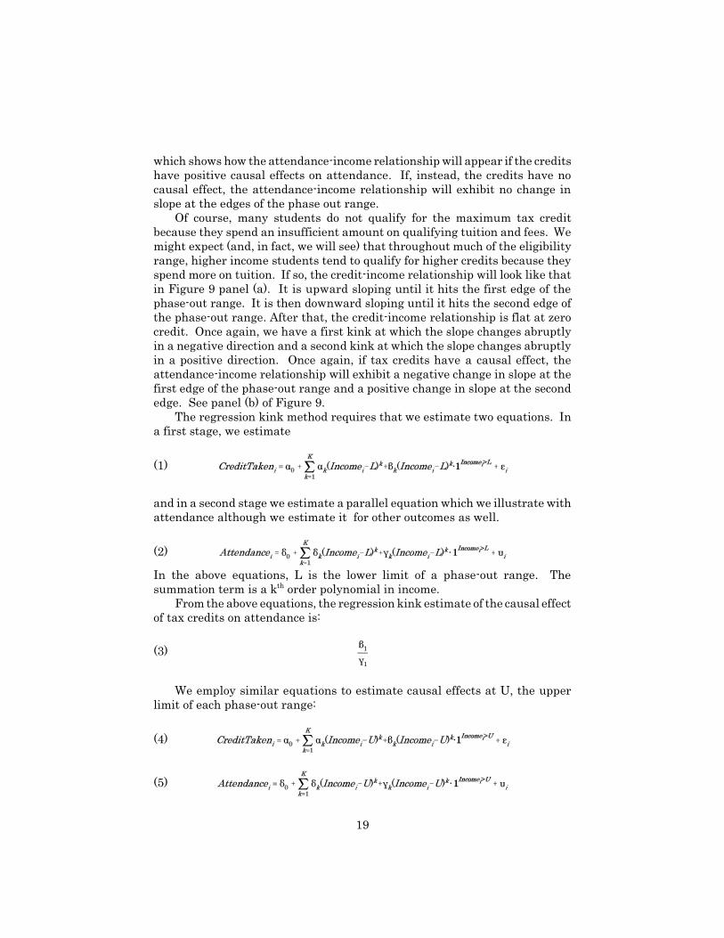
The regression kink method requires that we estimate two equations. Ina first stage, we estimate

(1)

and in a second stage we estimate a parallel equation which we illustrate withattendance although we estimate it for other outcomes as well.

(2)

In the above equations, L is the lower limit of a phase-out range. Thesummation term is a k order polynomial in income.th

From the above equations, the regression kink estimate of the causal effectof tax credits on attendance is:

(3)

We employ similar equations to estimate causal effects at U, the upperlimit of each phase-out range:

(4)

(5)

19

11111So far, we have used stylized figures to illustrate how the regression kinkmethod works. Now consider how data actually appear. Figure 10 shows theempirical credit-income relationship in 2007 and in 2011 for students who aredependents in households that file jointly. In both years, credits rise smoothlywith income until the first edge of the phase-out range. This sweeping curvereflects higher income students' tendency to pay more tuition. At the firstedge, the relationship abruptly becomes very negative and nearly linear,indicating that the phase-out formula is dictating the relationship. At thesecond edge, the slope of the credit-income relationship abruptly changes againfrom negative to flat. Thus, Figure 10 looks very much like the stylizedexample in panel (a) of Figure 9.

Although we have not shown it for reasons of conciseness, the credit-incomerelationship looks very similar for every year from the introduction of thecredits though 2012. The relationship also looks similar for single filers, asopposed to married couples filing jointly. There is always a sharp negativechange in the slope of the credit-income relationship at the lower edge and asharp positive change in the slope at the upper edge. Only the height of thecredit and location of the phase-out range changes.

Figure 10 shows close-ups of the kinks in the empirical credit-incomerelationship. These close-ups may seem unnecessary for displaying the kinksbecause they are very obvious. However, the regression kink method candepend on small changes in slopes at the edges of the phase-out range. Therefore, close-ups are useful for examining the empirical relationshipsbetween outcomes, like attendance, and income.

We have seen that the credit-income relationship exhibits sharp kinks justas in the stylized example. Do outcome-income relationships similarly matchwhat we would expect if the credits have causal effects? Figures 11 through 13show that the answer is no. The students in Figure 11 correspond to those onwhom Figure 10 is based yet we see no change whatsoever in the slope of theircollege attendance-income relationship at the edges of the phase-out range. (The close-ups are helpful here.) Perhaps, however, students are not changingwhether they attend college but are changing where they attend college. Thetax credit might, for instance, allow them to attend a four-year college ratherthan a two-year college. It might allow them to attend a college with higherinstructional resources. We look for evidence of such "upgrading" in Figures12 through 14 but we see none. At the edges of the 2011 phase-out range, wedo not perceive changes in the slope of the four-year college attendance-incomerelationship, the two-year college attendance-income relationship, or theinstructional resources-income relationship. Perhaps the tax credit changesthe grants and scholarships a student receives rather than his attendance? Figure 15 suggests not. It shows no perceptible changes in the slope of the

20

grants-income relationship at the edges of the phase-out range.15

Of course, we should not rely exclusively on our visual ability to discernchanges in slopes at the edges of the phase-out range. Therefore, we show theresults of formal regression kink analysis in Tables 13 and 14.

Table 13 shows estimates of the first stage equations--that is, estimates of

1â from equations (1) and (4) above. Each equation is estimated for 19 and 20year olds in the year mentioned using a bandwidth of plus or minus $3,000around the location of the kink mentioned. The results shown are for a cubicpolynomial following the guidance given by Ganong and Jäger (2014). Although we do not show alternative specifications, the first stage estimatesare, in fact, highly robust to our (i) changing the degree of the polynomial, (ii)expanding the bandwidth around each kink as far as plus or minus $10,000,(iii) focusing on older students, (iv) estimating the equations on years otherthan 2007 and 2011.16

Each estimated coefficient in Table 13 should be interpreted as the changein the slope of the credit-income relationship that occurs at the kinkmentioned. Thus, for instance, -0.107 in the first row tells us that the slope ofthe credit-income relationship decreases by about 11 cents per dollar at thelower edge of the phase-out range for joint filers in 2011. This makes a greatdeal of sense and corresponds closely to what we saw in the Figure 10 close-up. The credit-income relationship is almost flat at a credit of about $2,200 as itapproaches the lower edge. The relationship then falls fairly linearly so thatthe entire $2,200 goes to zero smoothly over a $20,000 income interval. Thismeans that, just from the figure, we expect the slope to fall from approximatelyzero to approximately -0.11. This is exactly what it does. All of the estimatedcoefficients in Table 13 can be similarly interpreted and line up similarly withwhat we expect based on the credit formula. For context, we have included17

a column showing the coefficient we would expect if credit-income relationshipwere flat at the maximum possible credit when approaching the lower edge ofthe phase-out range. Of course, students are not generally at the maximumcredit and the relationship need not be flat approaching the phase-out range. Nevertheless, these expected coefficients are a reminder of the sign we expectand the maximum magnitude consistent with the formula.

We use selected data from the population of individuals to produce theestimates in Table 13. Therefore, standard errors and p-values should not be

For conciseness, we show certain outcome-income relationships for 2011 only. 15

However, they are available from the authors for all outcomes in all years. We do not mean that the estimated coefficients do not change. We expect them to16

change with the year and the individuals' age because the credit formula that applieschanges with year and age. Rather, we mean that the estimated coefficients are alwaysclose to what we expect based on the formula that applies.

We do not show estimates for kinks at which there is insufficiently dense data. For17

instance, there are insufficient independent, young filers at the upper edge of the singleand joint phase-out ranges.

21

interpreted using a conventional sampling framework. Moreover, theregression kink method employs a specification that imposes very littleeconomic modeling so it is not easy to interpret the standard errors asmisspecification of the model as proposed by Abadie, Athey, Imbens, andWooldridge (2013). Nevertheless, we show p-values associated with the robust-to-heteroskedascity standard errors suggested by Card, Lee, Pei, and Weber(2012) in their seminal paper on regression kink methods.

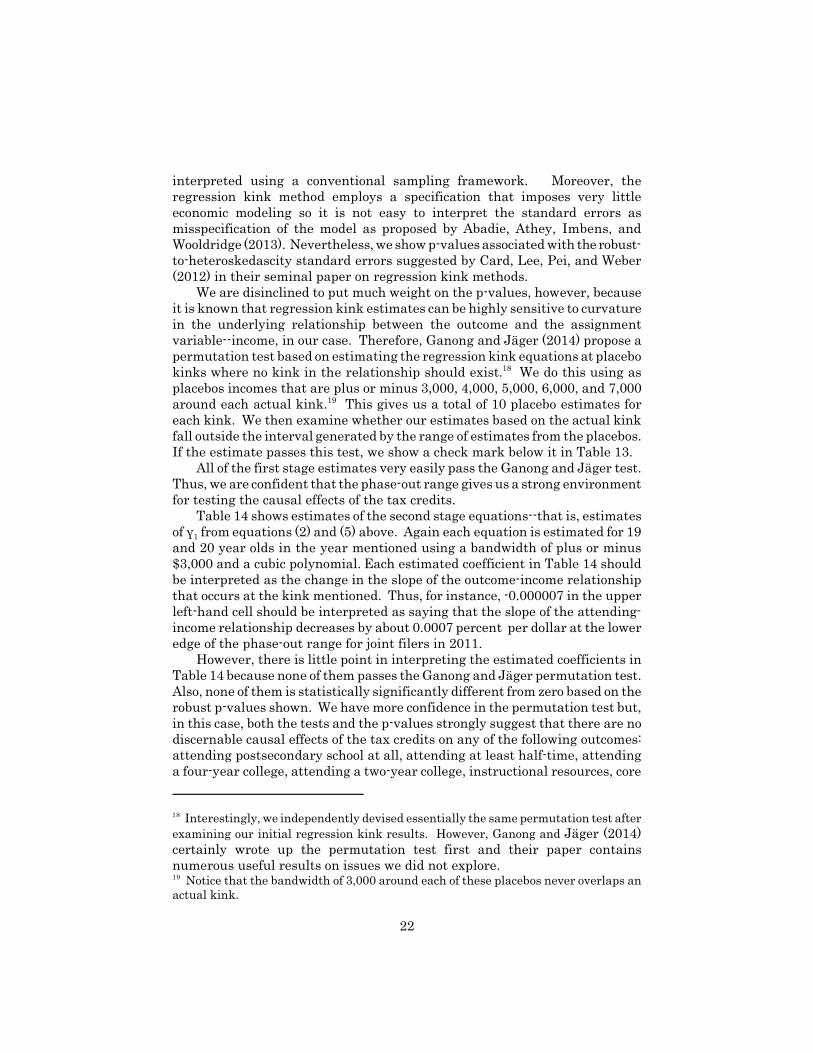
We are disinclined to put much weight on the p-values, however, because it is known that regression kink estimates can be highly sensitive to curvaturein the underlying relationship between the outcome and the assignmentvariable--income, in our case. Therefore, Ganong and Jäger (2014) propose apermutation test based on estimating the regression kink equations at placebokinks where no kink in the relationship should exist. We do this using as18

placebos incomes that are plus or minus 3,000, 4,000, 5,000, 6,000, and 7,000around each actual kink. This gives us a total of 10 placebo estimates for19

each kink. We then examine whether our estimates based on the actual kinkfall outside the interval generated by the range of estimates from the placebos. If the estimate passes this test, we show a check mark below it in Table 13.

All of the first stage estimates very easily pass the Ganong and Jäger test. Thus, we are confident that the phase-out range gives us a strong environmentfor testing the causal effects of the tax credits.

Table 14 shows estimates of the second stage equations--that is, estimates

1of ã from equations (2) and (5) above. Again each equation is estimated for 19and 20 year olds in the year mentioned using a bandwidth of plus or minus$3,000 and a cubic polynomial. Each estimated coefficient in Table 14 shouldbe interpreted as the change in the slope of the outcome-income relationshipthat occurs at the kink mentioned. Thus, for instance, -0.000007 in the upperleft-hand cell should be interpreted as saying that the slope of the attending-income relationship decreases by about 0.0007 percent per dollar at the loweredge of the phase-out range for joint filers in 2011.

However, there is little point in interpreting the estimated coefficients inTable 14 because none of them passes the Ganong and Jäger permutation test. Also, none of them is statistically significantly different from zero based on therobust p-values shown. We have more confidence in the permutation test but,in this case, both the tests and the p-values strongly suggest that there are nodiscernable causal effects of the tax credits on any of the following outcomes: attending postsecondary school at all, attending at least half-time, attendinga four-year college, attending a two-year college, instructional resources, core

Interestingly, we independently devised essentially the same permutation test after18

examining our initial regression kink results. However, Ganong and Jäger (2014)certainly wrote up the permutation test first and their paper containsnumerous useful results on issues we did not explore.

Notice that the bandwidth of 3,000 around each of these placebos never overlaps an19

actual kink.

22

educational resources, the "list" tuition and fees of the student's college, thegrant and scholarships the student receives, and the tuition the student pays. (The last eight outcomes are all conditional on attending at all.)

We cannot rule out effects of the tax credits that are too small to bediscernable. For instance, if a $1,000 tax credit were to increase attending by1 percent, we would be unable to distinguish this effect from random noise. Generally, though, we interpret the estimates in Table 14 as strongconfirmation of what the figures suggest: the tax credits have no or at mostextremely small causal effects on college-related outcomes in the vicinity of thephase-out ranges.

The advantage of regression kink analysis is that, so long as theassumptions of the method are met, it produces estimates that are verycredibly causal. The disadvantage is that the estimates are relevant only forhouseholds with incomes near the phase-out regions. Owing to the changes inthe phase-out ranges, especially the major rise in the ranges that accompaniedthe AOTC, we have estimates for married joint filers that cover a rather widearray of incomes: from about $107,000 to $180,000 in 2013 dollars. For singlefilers, we have regression kink estimates than span incomes from about$53,000 to about $90,000 in 2013 dollars. We find no causal effects of the taxcredits over these fairly wide regions.

However, the phase-out range never occurs in the lower to middlingpercentiles of the income distribution and, therefore, we cannot extrapolatefrom the regression kink estimates to say that removing or reducing the taxcredits would have no or only a slight effect on college attendance by studentswhose families have earnings at, say, the 50th percentile for their filing status. There is no reason to think that the effects on them will be as modest as theyare around the phase-out range. Indeed, a policy maker who is trying tominimize the causal effects of withdrawing a tax credit might choose to phaseit out among precisely those households who are likely to be unaffected. Thisdoes not imply that all households would be similarly unaffected.

6.2 Using the Introduction of the AOTC to Identify the CausalEffects of Tax Credits Across All Eligible IncomesBecause we cannot extrapolate our regression kink estimates to low and middleincome households, we turn to the introduction of the AOTC which, as we haveseen, sharply increased the generosity of the education tax credits for somehouseholds. In this section, we employ the classic method of analyzing how thechange in college-going behavior, from cohort to cohort, is related to the changein the tax credits they experience. Because the introduction of the AOTCaffected students across a very wide range of incomes, including poor students,the estimates from this method have broad application.

This method can be embodied in the simple equation:

(6)

23

1where ë is the coefficient of interest, there is a polynomial in income, and thereis a full set of year effects. Because we estimate this equation for individualsof certain ages (such as 19), we do not include cohort effects which would beredundant.

Because the tax credits that the household actually takes may reflect itsresponse to the tax credits (for instance, receiving a larger credit because thecredit causes one to attend a more expensive school) and not just the policy-driven change in the credits, we construct a simulated instrument for each taxcredit. A properly constructed simulated instrument embodies the policy-driven change in the credit, holding the household's behavior constant. Thus,our simulated instrument is the credit the household would receive if itscollege-going choices were typical for a household of its income in a base year(which we set to be 2008). These typical choices are run through the laws ofthe actual year so that the instrument reflects the changes in the tax creditparameters and only the tax credit parameters. An especially simple examplewould be the following. Suppose that households with $50,000 of income andone child aged 18 typically have a 50 percent probability of sending a child tocollege in such a way as to fulfill the requirements of the HTC (and thereforethe AOTC): at least half-time enrollment, enrollment in a degree or certificateprogram, and so on. Suppose that, conditional on its child enrolling, such ahousehold typically spends $4,000 on qualifying tuition and fees. Then, thesimulated instrument for the 2008 credit would be 50% × $1,800, and thesimulated instrument for the 2009 credit would be 50% × $2,500 in 2009.

Of course, computing the simulated instruments is more complicated butthe essential elements are clear. For each level of income, we need the taxcredit qualifying variables: spending on tuition and fees, half-time enrollment,taxes owed before the education credits, and so on.20

With the simulated instruments, we have a simple first stage equation:

(7)

When estimating equations (6) and (7), it is important to cluster thestandard errors to account for the fact that the tax credit policy is not

For each potential student cohort (those who are 19 in 2008, say), we divide their20

filers' income in each year into 300 quantiles for married filers and 300 quantiles forsingle filers. We then find the mean of each qualifying variable for each quantile. Weuse these means to construct the simulated instrument for the tax credits by runningthem through the credit formulae that apply in each year. A student is assigned to aquantile based on his filer's income when he is 17. After that, the filer's qualifyingvariables are made to evolve with those of his quantile. This excludes all possibility ofendogeneity. We choose 300 quantiles because it puts about 5,000 households in eachquantile--enough households to generate precise measures of their average behavior. Additional details are available from the authors.

24

individual-specific. For instance, consider two households each of which spends$4,000 on tuition in 2008. If both households have incomes below $96,000 andowe at least $2,500 in taxes before credits, these households will experience thesame change in credits due to the introduction of the AOTC even if they havequite different incomes--$60,000 and $95,000, say. To generate the clusters,we run each household through the tax credit formulae in 2008 and 2009. Weput households in the same cluster if they receive identical tax credits whenthey make the same college attendance and payment choices.

The weakness of the simulated instrumental variables method, which isoften used to assess tax reforms, is that its estimates may reflect other eventsthat occur at the same time as the change in the tax credits and that affect thesame people who experience a change in tax credits. Given that the AOTC wasintroduced as part of the stimulus package, one might worry that certainhouseholds were either affected by the events that triggered the stimulus (thefinancial crisis, the rise in unemployment) or by other components of thestimulus bill. For instance, college enrollment has often been found to be anti-cyclical owing to the decrease in opportunity costs (that is, labor earnings)during downturns. So, we might expect enrollment to rise in 2009 regardlessof the credits. Or families who lost home equity in 2008 may have found itharder to finance college.

Despite these circumstances, we are fairly confident that our estimatesbased on the introduction of the AOTC bear a causal interpretation. Ourconfidence is based on three things. First, the AOTC increased tax credits notjust for low-income or high-income households but for both types of households. Indeed, as we show below, the changes in the tax credits are not a simplefunction of household income. Some "control" (unaffected or hardly affected)households have high incomes; some have relatively low incomes. Some of themost affected households have fairly high incomes; some have low incomes. Our second reason for confidence is that trends in college-going behavior wereparallel before and after the law change, not just for students as a whole butwhen we define groups who were more and less affected by the change in taxcredits. Our third reason for confidence is that this method produces resultsthat closely match the regression kink results for households in the incomeranges covered by those results.

Figures 16 through 18 demonstrate our point that the changes induced bythe AOTC were not a simple function of income. To construct these figures, wesubtract each of the 2008 figures from section 2 from its 2009 counterpart. This shows us the change in the tax credit available to a household with agiven amount of spending on tuition, for each level of income. For instance,Figure 17 shows the change in the tax credit available to a household that filesjointly, that has no dependent other than the prospective student, and thatwould spend $4,000 on qualified tuition and fees if its child were to attendcollege. In zone (a) of the figure, we see that households with incomes up toabout $35,000 ($30,000 for third and fourth year students) experience a largeincrease of about $1,000 in tax credits owing to the AOTC's refundability. In

25

zone (b), households with incomes from about $40,000 to $96,000 experience amodest increase of $500 if their student is in his first or second year. Theyexperience a very large increase of $1,700 if their student is in his third orfourth year. In zone (c), households with incomes from $116,000 to about$160,000 experience a tremendous increase of $2,500 in their tax creditregardless of the year of their student. This is because they are above thephase-out range for the TCLL and HTC but not for the AOTC. Finally,households in zone (d) with incomes of $180,000 and above experience zerochange in the tax credits they could take.

Figures 16 and 18 show similar change in tax credit graphs for householdswho spend, respectively, $10,000 and $2,400 on tuition on fees. One can seethat the most and least affected households are somewhat different than inFigure 17. Indeed, there is variation in treatment not only as we scan thefigures horizontally (across incomes) but also as we scan them vertically--across the second versus third year of college. Below, we refer to zones athrough d in Figures 16 through 18 so we encourage readers to fix them intheir minds.

In econometric terms, it is helpful to have all this variation in the locationof the most affected and least affected households because it means that thetreatment and control groups have fairly common support, in terms of theincome distribution. Put another way, we can compare high income householdswho are greatly treated because they are just inside the top end of the newphase out range with other high income households who experience notreatment because they are just outside the top end of the phase out range. Weneed not compare high-income households only to low-income households. Similarly, we can compare upper-middle income households who are greatlytreated because they are just outside of the upper limit of the old phase outrange with households who are only modestly treated because they are justinside the upper limit of the old phase out range. And so on.

In addition, we gain a great deal of econometric common support from the"vertical" differences due to the AOTC (but not the HTC) being available tothird and fourth year students.

Although the variation in tax credits between 2008 and 2009 is too complexto be reasonably described as differences-in-differences, the logic of ourempirical strategy is essentially that of differences-in-differences. That is, weare simultaneously exploiting differences across cohorts and differences withincohorts in the tax credits that apply to them. An important test of such aidentification strategy is whether the groups who are differentially treated bythe law change are on parallel trends prior to the law change. If they are ontrends that are fairly parallel, the method is usually reliable. If they are ondiverging trends, the estimates may spuriously reflect the divergence in theirpreexisting trends.

In Figures 19 through 22, we show trends in college attendance and otheroutcomes by income group, where each group is set up to be as close as possibleto the edge of one of the zones mentioned above. Thus, in each figure, the panel

26

for 19-year-olds has a group from the top of zone a ($25,000-35,000, experienceda moderate increase in credits) whom one would naturally compare to thebottom of zone b ($40,000-50,000, experienced only a slight increase in credits). It also has a group from the top of zone b ($86,000-96,000, experienced only aslight change) whom one would naturally compare to the bottom of zone c($116,000-126,000, experienced an extremely large increase). It finallycontains a group from the top of zone c ($150,000-160,000, experienced anextremely large increase) whom one would naturally compare to the bottom ofzone d ($180,000-190,000, entirely unaffected by the introduction of the AOTC).

In all of Figures 19 through 22, the pairs whom we need to be on paralleltrends are on parallel trends as we approach 2008, both for 19-year-olds and23-year-olds. All income groups are slightly affected by the business cycle, butthe effects tend to be parallel. Another way to see the parallel trends is togroup people by the change in tax credits that they experience if they behaveas they do in the base year. That is, the next figure is set up to show thevariation that will, through the simulated instruments, drive the estimates. For instance, for 19-year-olds, the groups are 0 change, a $1 to $500 increasein the simulated tax credit, a $501 to $750 increase, a $751 to $900 increase,and a $901 and greater increase. Figure 23 shows the trends for attendanceand other outcomes for 19 year olds when individuals are grouped that way. The figure demonstrates that people who were more and less affected by thetax credit changes were not previously on divergent attendance trends prior tothe introduction of the AOTC. (We can show similar figures for other outcomesand people of other ages.)

Indeed, Figures 19 through 23 not only show parallel trends prior to theAOTC. They show parallel trends right through the introduction of the AOTC.That is, the figures provide little evidence that people who experienced muchlarger increases in tax credit generosity had college outcomes that were anydifferent as a result.

In Tables 15 and 16 we formalize this finding by showing estimates ofequations (6) and (7). Each regression contains a quintic polynomial inadjusted gross income as well as a full set of year effects. To maximize21

statistical power, we use the three years before and three years after theintroduction of the AOTC: 2006 through 2011. However, the results are verysimilar if we use only 2008 and 2009. We show results for 19-year-olds and 23-year-olds. The results for individuals of ages 20 through 22 and ages 24through 26 are similar. As we have seen, older people are much less affectedby the AOTC so it is not worthwhile analyzing them.

Table 15 shows the first stage regressions in which the actual tax creditsa person takes are regressed on her simulated instrument. There are multiplecolumns only because the individuals over whom the first stage is estimatedvaries slightly with the outcomes under study. Most of the coefficients for 19-

The results are very similar if we use polynomials from a cubic upwards.21

27

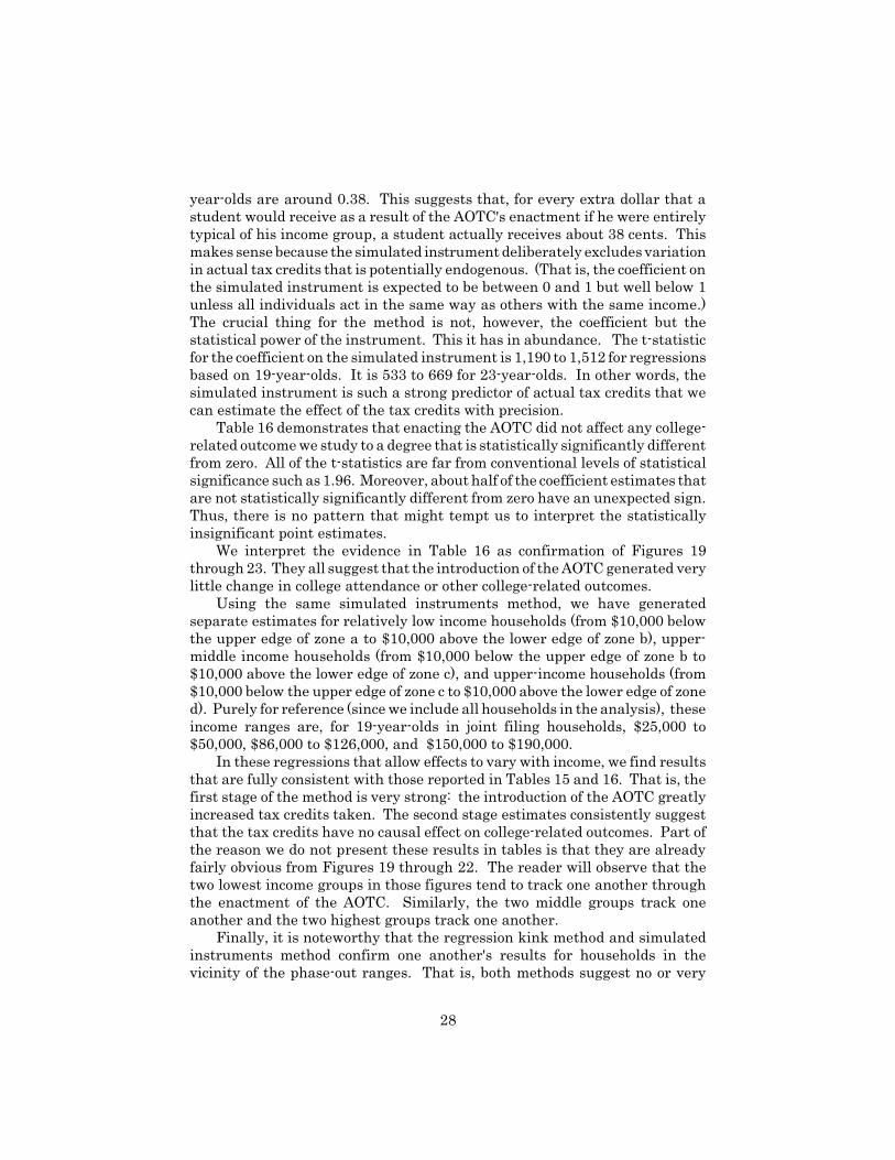
year-olds are around 0.38. This suggests that, for every extra dollar that astudent would receive as a result of the AOTC's enactment if he were entirelytypical of his income group, a student actually receives about 38 cents. Thismakes sense because the simulated instrument deliberately excludes variationin actual tax credits that is potentially endogenous. (That is, the coefficient onthe simulated instrument is expected to be between 0 and 1 but well below 1unless all individuals act in the same way as others with the same income.) The crucial thing for the method is not, however, the coefficient but thestatistical power of the instrument. This it has in abundance. The t-statisticfor the coefficient on the simulated instrument is 1,190 to 1,512 for regressionsbased on 19-year-olds. It is 533 to 669 for 23-year-olds. In other words, thesimulated instrument is such a strong predictor of actual tax credits that wecan estimate the effect of the tax credits with precision.

Table 16 demonstrates that enacting the AOTC did not affect any college-related outcome we study to a degree that is statistically significantly differentfrom zero. All of the t-statistics are far from conventional levels of statisticalsignificance such as 1.96. Moreover, about half of the coefficient estimates thatare not statistically significantly different from zero have an unexpected sign. Thus, there is no pattern that might tempt us to interpret the statisticallyinsignificant point estimates.

We interpret the evidence in Table 16 as confirmation of Figures 19through 23. They all suggest that the introduction of the AOTC generated verylittle change in college attendance or other college-related outcomes.

Using the same simulated instruments method, we have generatedseparate estimates for relatively low income households (from $10,000 belowthe upper edge of zone a to $10,000 above the lower edge of zone b), upper-middle income households (from $10,000 below the upper edge of zone b to$10,000 above the lower edge of zone c), and upper-income households (from$10,000 below the upper edge of zone c to $10,000 above the lower edge of zoned). Purely for reference (since we include all households in the analysis), theseincome ranges are, for 19-year-olds in joint filing households, $25,000 to$50,000, $86,000 to $126,000, and $150,000 to $190,000.

In these regressions that allow effects to vary with income, we find resultsthat are fully consistent with those reported in Tables 15 and 16. That is, thefirst stage of the method is very strong: the introduction of the AOTC greatlyincreased tax credits taken. The second stage estimates consistently suggestthat the tax credits have no causal effect on college-related outcomes. Part ofthe reason we do not present these results in tables is that they are alreadyfairly obvious from Figures 19 through 22. The reader will observe that thetwo lowest income groups in those figures tend to track one another throughthe enactment of the AOTC. Similarly, the two middle groups track oneanother and the two highest groups track one another.

Finally, it is noteworthy that the regression kink method and simulatedinstruments method confirm one another's results for households in thevicinity of the phase-out ranges. That is, both methods suggest no or very

28

small causal effects of the tax credits on college outcomes.

7 Federal and Social Returns to the Investment in the TaxCreditsWe would like to compute various rate of return on investment calculations forthe tax credits. However, given that they appear to have little or no causaleffect on college-going, the exercise would be nugatory. Regardless of how wemake the calculation, we will find that the U.S. Treasury will recoup none ofthe spending on the higher education tax credits through higher future taxpayments.

Since the tax credits cannot generate effects on other outcomes interestingto the federal government (such as crime) if they do not first affect educationaloutcomes, we will also necessarily find that the federal government as a wholewill recoup none of the spending on the higher education tax credits.

Finally, education can have social returns as well as private returns. Forinstance, one person's education may improve that of her children or neighbors.A more educated person may be a better civic participant. Nevertheless, themechanisms for social returns all rely on a policy actually affecting educationattainment in some way. Thus, regardless of how education generates socialreturns, we will necessarily find that society will earn a zero return on the taxcredits.

In 2014, the federal government and society spent $23 billion on taxcredits, an increase of about $15 billion or 177 percent since 2008 (in realdollars). Since we closely study the period from 2006 onwards, our findings canfairly confidently be interpreted as evidence that this increase in tax credits isunlikely to be recouped.

Because we do not have data to study the initial enactment of the taxcredits, we can be less confident about the $8.3 billion that the federalgovernment was already spending in 2008. That is, it is possible that this $8.3billion has causal effects on collegiate attainment and will be recouped withinterest. However, there is at best weak evidence in favor of this possibility. Neither the regression kink estimates from 2007 nor Long's estimates supportthis interpretation. Moreover, such an argument would have to rely on theidea that the $8.3 billion was targeted at precisely those households most likelyto be affected--that is, those with incomes of $40,000 to about $93,000 in 2008. If this targeting story were correct, however, it would be surprising that wefind no evidence of effects either at the lower end of this range (upper zone ato lower zone b) or the higher end of this range (upper zone b to lower zone cwhere simulated instrument as well as regression kink estimates areavailable). Nevertheless, we cannot rule out the possibility that the pre-AOTCtax credits had substantial effects on collegiate attainment right in the middleof this income range--$60,000 to $80,000, say. If this were to be the case, whichseems unlikely, it would suggest that the highest return on investment wouldbe attained if the federal government were to focus higher education tax creditson this specific income range, giving credits not much more generous than the

29

2008 HTC and TCLL. Overall, we conclude that there are shaky evidential foundations for

arguments based on the idea that the Treasury, federal government, or societywill recoup the tax credits with interest through higher education investments.

Of course, none of this means that the tax credits are wasted. They aresimply a transfer from some individuals to others. If there is some way otherthan higher education in which the people who receive the transfers employmoney in a way that is especially helpful to society or to the federal budget, thetax credits may be somewhat recouped through this other channel. However,we are not aware of clear hypotheses about channels other than highereducation.

8 Discussion and ConclusionsThere are at least four possible explanations for the tax credits' meager

effects on college-going: the credits are offset by decreased financial aid; thecredits are offset by increased tuition and fees; eligible individuals are notliquidity constrained with regard to college-going; the credits are structured ina way that minimizes their causal impact. Consider these explanations inturn.

If every increase in the generosity of the higher education tax credits isoffset by a corresponding decrease in financial aid, we would expect the creditsto have few or no effects on college. The tax credits would serve merely as atransfer to state governments and private philanthropies that would haveprovided the aid and can now use the funds for other purposes. However, wefind no evidence of such offset so it is unlikely to be an important reason whythe tax credits have few effects on college-going.

There is a long-standing hypothesis (the "Bennett Hypothesis") thatincreased federal support for higher education (in all forms) causes tuition torise, thereby limiting the effect on college-going. That is, the supply of highereducation might be inelastic so that the increased federal support would triggera price, not a quality, response. The price response need not occur throughindividual institutions raising their tuition. Students could be unable to findseats at inexpensive public or non-profit colleges that are supply constrained. They might enroll instead at for-profit schools that charge higher tuition. However, we do not find any evidence that the tax credits induce students toattend schools with higher list tuition or to pay higher tuition conditional onattending. Thus, our results provide no support for the Bennett Hypothesis asan explanation of the tax credits' inefficacy.

If individuals are not liquidity constrained when making college choices,they will exhibit approximately the same college-going behavior with orwithout the tax credits. The credits will simply reduce their borrowing orincrease their saving. It may well be that households with incomes at or abovethe HTC/TCLL phase-out range are unconstrained. If they are, the regressionkink analysis will indicate no effects and the AOTC's great rise in the locationof the phase-out (from $96,000-116,000 to $160,000-180,000) will have

30

produced no effects in the simulated instrument analysis. A lack of liquidityconstraints is a less obvious explanation for the refundable AOTC's lack ofeffect on low-income households. However, even they may be unconstrainedowing to their being eligible for grants (most obviously the Pell Grant), work-study, and loans at interest rates well below what a truly private lender wouldcharge. While the Pell Grant and federal loans cannot cover the cost of22

America's most selective non-profit colleges for a low-income student, suchcolleges offer generous financial aid to low-income students who meet theirstringent academic criteria. Thus, all in all, we consider a lack of liquidityconstraints to be plausible explanation for the tax credits' inefficacy.

The structure of the tax credits may also contribute to their inefficacy. This possibility has been discussed and even appear in the debates thatpreceded the enactment of the HTC and TCLL. First, a household receives23

a credit only after spending money on tuition and fees. This timing guaranteesthat credit takers are those who do not have tight liquidity constraints. Second, the tax filer gets the credit, and the filer is very often not the student. This would not matter if the filer and student shared unified liquidityconstraints, but they might not. For instance, a student might be liquidityconstrained from attending the college of his choice and his parents mightleave him in this position although they themselves are not liquidityconstrained. If they get a tax credit, his parents buy a more expensive car ortake out a smaller mortgage. They are not obliged to use the money to relaxthe liquidity constraints affecting their child. Third, the tax credits may notbe terribly salient at the times when families are making college-goingdecisions. Although the formula for each credit is simple and IRS materials onthe credits are readily available, a family planning its finances might overlookthe credits because calculating them requires a number of steps (see Davis2002). Or, a family may discount the credits because they are uncertain--theycan depend on income that has not yet been realized at the time whenenrollment decisions are made.

Because the tax credits have always had the same basic structure (timing,recipient, information required for their calculation), we cannot readily assesswhether changing the credits' structure would change their efficacy. Experiments in informing people about them are ongoing, but the structural24

issues may go beyond a mere lack of information. The issues may be inherentlydifficult to address through the tax system unless filers are given some meansto anticipate the credits and to pre-designate them for college expenses. Devising such means is within the scope of what is practical--a sort of

We mean a private lender who accounted for borrowing risk and had no government22

guarantee to help enforce repayment. See, for instance, Lederman (1997), Hoxby (1998), Davis (2002), Long (2004),23

Dynarski and Scott-Clayton (2006), Kane (1997), Maag and Rohlay (2007), and Turner(2011).

The source is authors' personal communication with the researchers.24

31

"Advance" HTC, TCLL, or AOTC analogous to the Advance Earned Income TaxCredit. However, only a small share of people who were eligible for the EarnedIncome Tax Credit took it in the form of an advance, and the Advance EarnedIncome Tax Credit was eliminated in 2010 because its disadvantages were seento outweigh its advantages.25

Recall that at least some proponents of the higher education tax creditssuggested that they were simply intended as a middle-class tax cut. To thispoint, we saw in Tables 3 through 12 that most of the tax expendituresassociated with the credits do go to middle-income households. This is less truenow, with the AOTC, than it was in 1999 through 2008. Nevertheless, middle-income households remain the key recipients of the tax expenditures.

It is far beyond the scope of this paper to evaluate the incidence orefficiency of the higher education tax credits if we view them purely as middle-class tax cuts, setting aside their links to education investments. However, itis useful to make two points on the tax credits purely as tax cuts.

First, the tax credits raise marginal tax rates by as much as 12.5 to 25percentage points in the phase-out ranges. These are potentially importantmarginal rate increases. On the other hand, the credits lower marginal taxrates for households whose credits are limited by their taxes due. We can seefrom Figures 1 through 6 that these households tend to be in the 15 percent taxbracket. Nevertheless, over quite a wide region of the income distribution(especially under the AOTC), the credits do not affect marginal tax rates butonly average tax rates. Thus, anyone investigating whether the credits changetaxable income (labor supply) of middle-income households should focus on theminority of households whose marginal tax rates are affected.

Second, the tax credits interact with state and local support for highereducation in a manner that generates horizontal differences in the tax cuts formiddle-income households who exhibit essentially the same behavior. Forinstance, consider a state or locality that collects considerable sales tax revenueand uses it to subsidize tuition at its public postsecondary institutions. Itsfamilies would not pay much tuition because they have already paid "up front"through sales taxes. They would receive smaller federal tax credits thanfamilies with identical incomes who live in areas where public institutions havethe same total resources but where state and local governments choose tosubsidize tuition less by taxes collected "up front." This may seem like acontrived example but it is not. State and local policies dominate tuitionsetting in the U.S., and states differ greatly in the extent to which theysubsidize tuition through state and local taxes (Long 2004a). Since the federalgovernment is inevitably a minor player in higher education relative to thestates, it may not be possible to design horizontally equitable tax cuts throughthe means of higher education tax credits.

See General Accounting Office (2007).25

32

9 References

Abadie, Alberto, Susan Athey, Guido W. Imbens, and Jeffrey Wooldridge. 2013. "Finite Population Causal Standard Errors," Stanford Universitytypescript.

Bradford, David. 1984. Blueprints for Basic Tax Reform. Arlington, VA: TaxAnalysts.

Bulman, George. 2012. "The Effect of Access to College Assessments onEnrollment and Attainment," University of California-Santa Cruz typescript.

Card, David, David Lee, Zhuan Pei, and Andrea Weber. 2012. "NonlinearPolicy Rules and the Identification and Estimation of Causal Effects in aGeneralized Regression Kink Design." National Bureau of Economic ResearchWorking Paper 18564.

Crandall-Hollick, Margot L. 2013. Higher Education Tax Benefits: BriefOverview and Budgetary Effects." Congressional Research Service (R41967).

Crandall-Hollick, Margot L. 2012. "The American Opportunity Tax Credit:Overview, Analysis, and Policy Options" (R42561).

Davis, Albert J. 2002. "Choice Complexity in Tax Benefits for HigherEducation," National Tax Journal, 50 (3): 509–538.

Dynarski, Susan M., and Judith E. Scott-Clayton. 2006. "The Cost ofComplexity in Higher Education: Lessons from Optimal Tax Theory andBehavioral Economics," National Tax Journal, 59 (2): 319–356.

Hoxby, Caroline M. 1998. "Tax Incentives for Higher Education." in Poterba,James M. (ed.), Tax Policy and the Economy, Volume 12, 49–82. MIT Press,Cambridge, MA.

Ganong, Peter and Simon Jäger. 2014. "A Permutation Test and EstimationAlternatives for the Regression Kink Design," Harvard University typescript.

Joint Committee on Taxation. 2013. Estimates of Federal Tax Expendituresfor Fiscal Years 2012-2017 (JCS-1-13).

Joint Committee on Taxation. 2014. Estimates of Federal Tax Expendituresfor Fiscal Years 2014-2018 (JCX-97-14).

Kane, Thomas J. 1997. "Beyond Tax Relief: Long Term Challenges toFinancing Higher Education," National Tax Journal 50 (2): 335–349.

33

Klasik, Daniel. 2013. "The ACT of Enrollment: The College Enrollment Effectsof State-Required College Entrance Exam Testing." Educational Researcher42: 151-159.

LaLumia, Sara. 2012. "Tax Preferences for Higher Education and AdultCollege Enrollment," National Tax Journal, 65(1): 59-90.

Lederman, Douglas. 1997. "The Politicking and Policy Making Behind a$40-Billion Windfall," Chronicle of Higher Education, 44:14 (November 28).

Long, Bridget Terry. 2004a. "Does the Format of a Financial Aid ProgramMatter? The Effect of State In-kind Tuition Subsidies," Review of Economicsand Statistics, 86(3): 767–782.

Long, Bridget Terry. 2004b. "The Impact of Federal Tax Credits for HigherEducation." in Hoxby, Caroline M. (ed.), College Choices: The Economics ofWhich College, When College, and How to Pay For It. Chicago, IL: Universityof Chicago Press, 101–168..

Maag, Elaine, and Jeffrey Rohaly. 2007. "Who Benefits from the Hope andLifetime Learning Credit?" Tax Policy Center, Urban Institute and BrookingsInstitution, Washington, DC.

National Center for Education Statistics, Institute for Education Sciences, U.S.Department of Education. Integrated Postsecondary Education Data System. Enrollment, Finance, Residence and Migration, and InstitutionalCharacteristics files. 1996 through 2012 editions. Electronic data. Washington, DC: U.S. Department of Education, retrieved August 2014.

Stantcheva, Stefanie. 2014. "Optimal Taxation and Human Capital Policiesover the Life Cycle," Harvard University typescript.

Turner, Nicholas. 2012b. "Why Don't Taxpayers Maximize their Tax-BasedStudent Aid? Salience and Inertia in Program Selection" The B.E. Journal ofEconomic Analysis & Policy 11.1.

Turner, Nicholas. 2012a. "Who Benefits from Student Aid? The EconomicIncidence of Tax-Based Federal Student Aid," Economics of Education Review.

Turner, Nicholas. 2011. "The Effect of Tax-based Federal Student Aid onCollege Enrollment," National Tax Journal 64: 839-861.

U.S. General Accounting Office. 2007. Advance Earned Income Tax Credit,Low Use and Small Dollars Paid Impede IRS’s Efforts to Reduce HighNoncompliance (GAO-07-1110). Washington, DC: GAO Report to the Joint

34

Committee on Taxation.

U.S. Department of the Treasury, Internal Revenue Service. 1999 to 2013. Form 8863 and Instructions for Form 8863.

U.S. Department of the Treasury, Internal Revenue Service. 2013. Statisticsof Income-2011: Individual Income Tax Returns, Publication 1304 (Rev. 08-2013), Washington DC: Department of the Treasury, Internal RevenueService.

U.S. Department of the Treasury, Internal Revenue Service. 2014. Compliance Data Warehouse. electronic data.

35

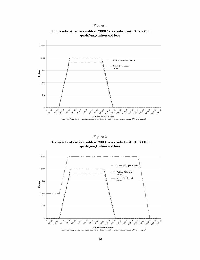
Figure 1

Figure 2

36

Figure 3

Figure 4

37

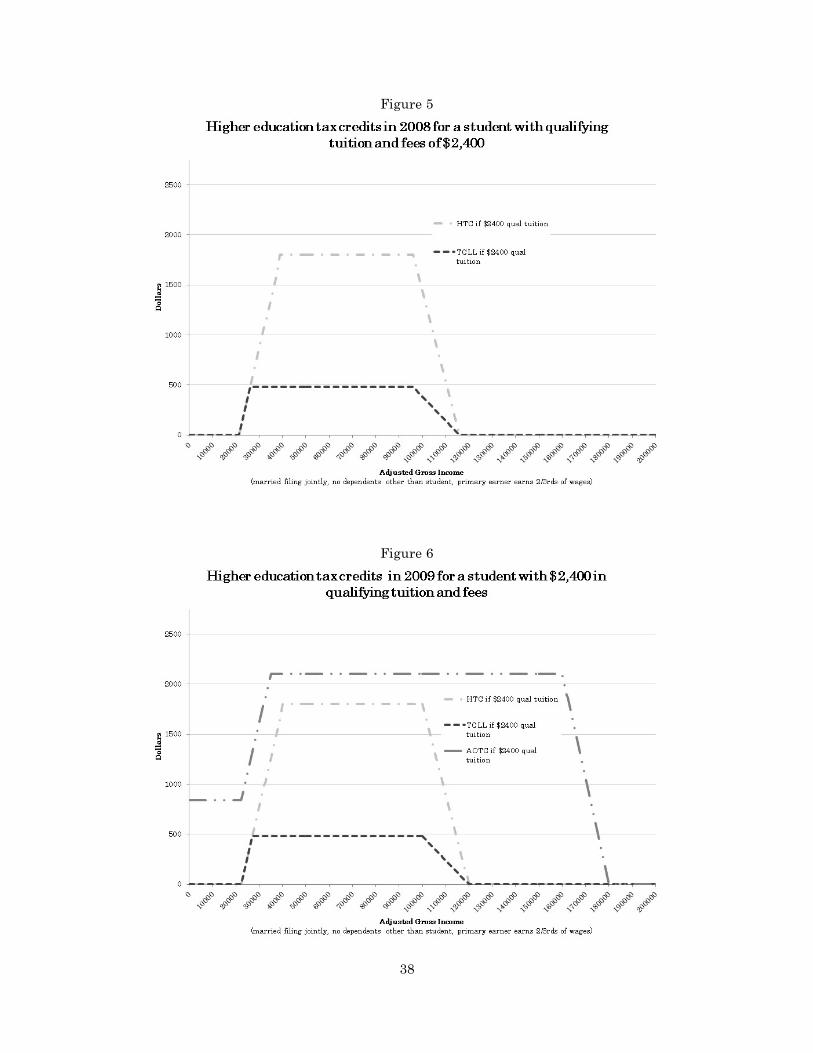
Figure 5

Figure 6

38

Figure 7

39

Figure 8

40

Figure 9

41

the tax credit-income relationship in 2011

overall

the tax credit-income relationship in 2007

overall

close-up on the phase-out range

close-up on the phase-out range

Figure 10

42

the attendance-income relationship in 2011

(attending at least half-time)

the attendance-income relationship in 2007

(attending at least half-time) close-up on the phase-out range

close-up on the phase-out range

Figure 11

43

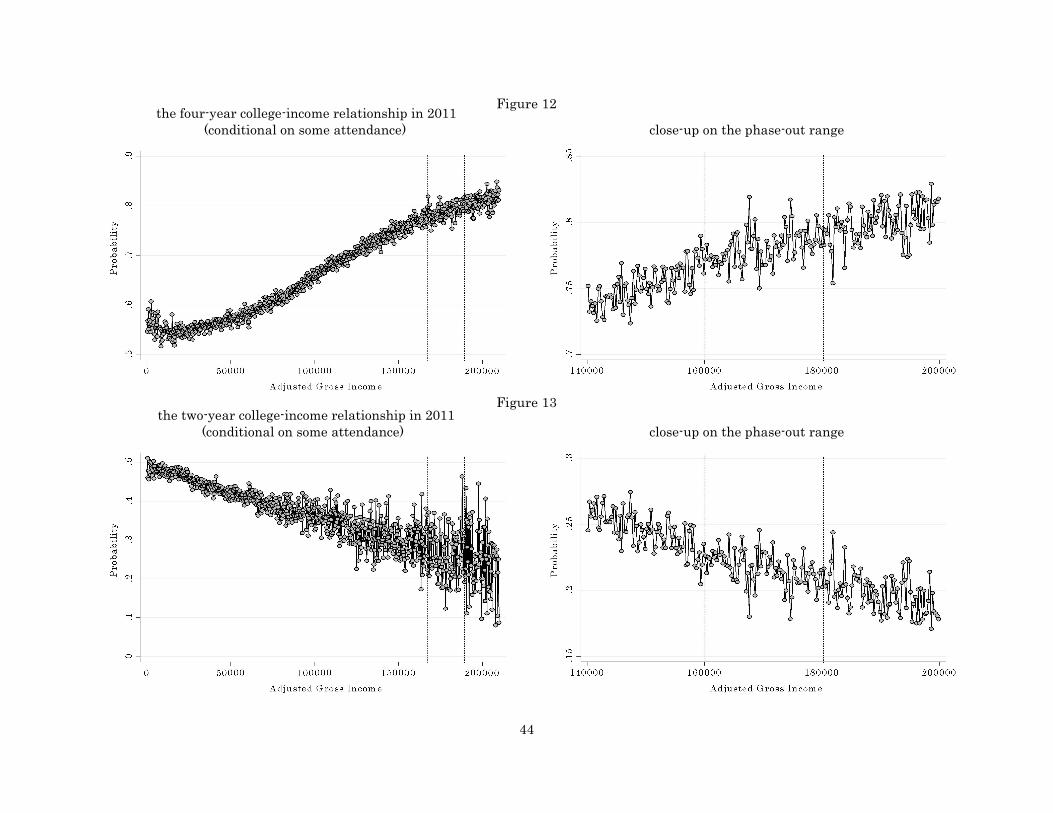
the four-year college-income relationship in 2011

(conditional on some attendance)

the two-year college-income relationship in 2011

(conditional on some attendance) close-up on the phase-out range

close-up on the phase-out range

Figure 12

Figure 13

44

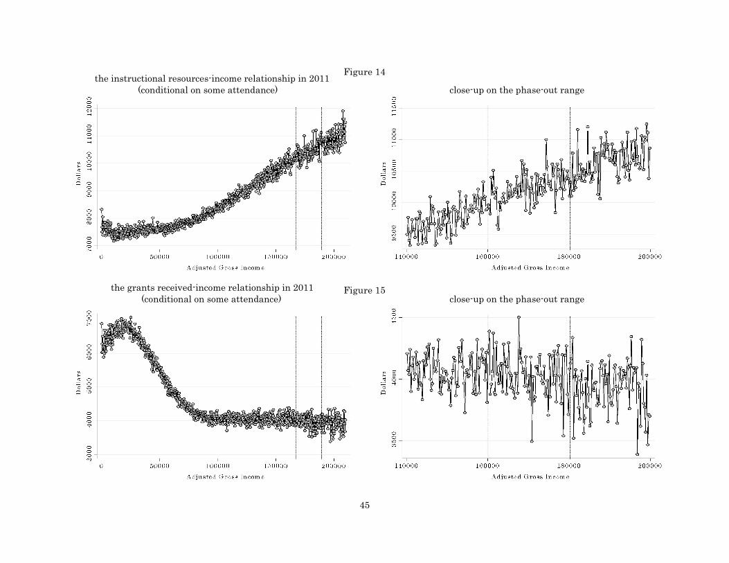
the instructional resources-income relationship in 2011

(conditional on some attendance) close-up on the phase-out range

the grants received-income relationship in 2011

(conditional on some attendance) close-up on the phase-out range

Figure 14

Figure 15

45

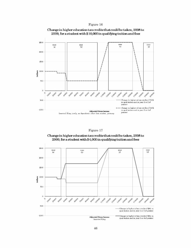
Figure 16

Figure 17

46

Figure 18

47

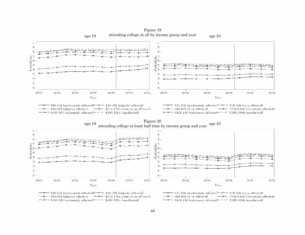
age 23age 19

age 19 age 23

Figure 19

attending college at all by income group and year

Figure 20

attending college at least half time by income group and year

48

age 19 age 23age 19 age 23

age 19 age 23

Figure 20

attending four-year college (conditional on attending)

Figure 21

attending two-year college (conditional on attending)

49

age 19 age 23

Figure 22

instructional resources (conditional on attending)w

50

attending college at all attending at least half-time

instructional resources (conditional on attending)attending four-year college (conditional on attending)

Figure 23

Outcomes of 19-year-olds by year and the degree to which they were potentially affected by the introduction of the AOTC

51

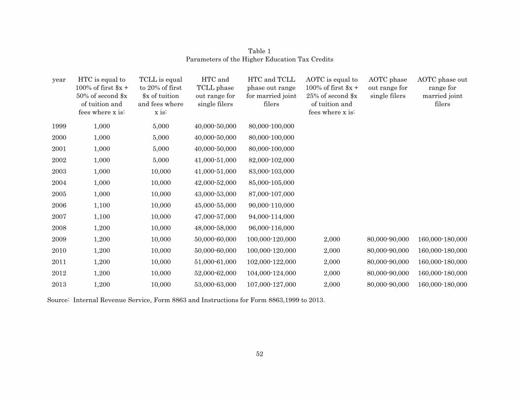
Table 1

Parameters of the Higher Education Tax Credits

year HTC is equal to

100% of first $x +

50% of second $x

of tuition and

fees where x is:

TCLL is equal

to 20% of first

$x of tuition

and fees where

x is:

HTC and

TCLL phase

out range for

single filers

HTC and TCLL

phase out range

for married joint

filers

AOTC is equal to

100% of first $x +

25% of second $x

of tuition and

fees where x is:

AOTC phase

out range for

single filers

AOTC phase out

range for

married joint

filers

1999 1,000 5,000 40,000-50,000 80,000-100,000

2000 1,000 5,000 40,000-50,000 80,000-100,000

2001 1,000 5,000 40,000-50,000 80,000-100,000

2002 1,000 5,000 41,000-51,000 82,000-102,000

2003 1,000 10,000 41,000-51,000 83,000-103,000

2004 1,000 10,000 42,000-52,000 85,000-105,000

2005 1,000 10,000 43,000-53,000 87,000-107,000

2006 1,100 10,000 45,000-55,000 90,000-110,000

2007 1,100 10,000 47,000-57,000 94,000-114,000

2008 1,200 10,000 48,000-58,000 96,000-116,000

2009 1,200 10,000 50,000-60,000 100,000-120,000 2,000 80,000-90,000 160,000-180,000

2010 1,200 10,000 50,000-60,000 100,000-120,000 2,000 80,000-90,000 160,000-180,000

2011 1,200 10,000 51,000-61,000 102,000-122,000 2,000 80,000-90,000 160,000-180,000

2012 1,200 10,000 52,000-62,000 104,000-124,000 2,000 80,000-90,000 160,000-180,000

2013 1,200 10,000 53,000-63,000 107,000-127,000 2,000 80,000-90,000 160,000-180,000

Source: Internal Revenue Service, Form 8863 and Instructions for Form 8863,1999 to 2013.

52

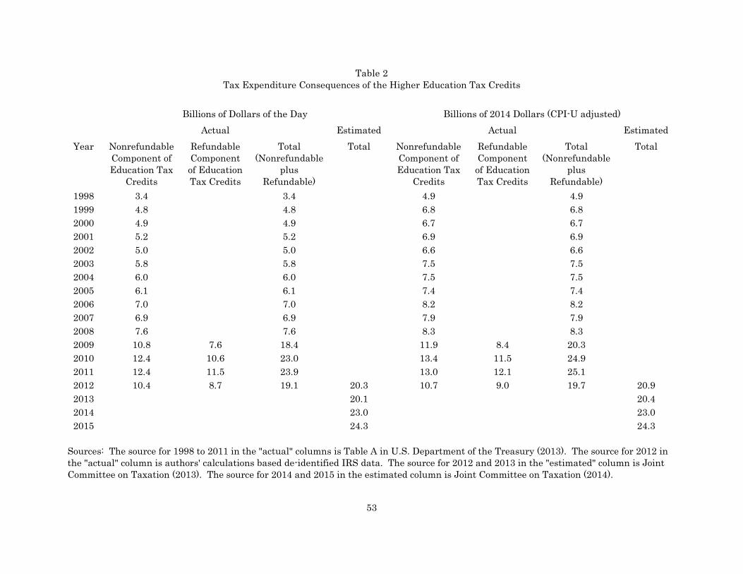
Table 2

Tax Expenditure Consequences of the Higher Education Tax Credits

Billions of Dollars of the Day Billions of 2014 Dollars (CPI-U adjusted)

Actual Estimated Actual Estimated

Year Nonrefundable

Component of

Education Tax

Credits

Refundable

Component

of Education

Tax Credits

Total

(Nonrefundable

plus

Refundable)

Total Nonrefundable

Component of

Education Tax

Credits

Refundable

Component

of Education

Tax Credits

Total

(Nonrefundable

plus

Refundable)

Total

1998 3.4 3.4 4.9 4.9

1999 4.8 4.8 6.8 6.8

2000 4.9 4.9 6.7 6.7

2001 5.2 5.2 6.9 6.9

2002 5.0 5.0 6.6 6.6

2003 5.8 5.8 7.5 7.5

2004 6.0 6.0 7.5 7.5

2005 6.1 6.1 7.4 7.4

2006 7.0 7.0 8.2 8.2

2007 6.9 6.9 7.9 7.9

2008 7.6 7.6 8.3 8.3

2009 10.8 7.6 18.4 11.9 8.4 20.3

2010 12.4 10.6 23.0 13.4 11.5 24.9

2011 12.4 11.5 23.9 13.0 12.1 25.1

2012 10.4 8.7 19.1 20.3 10.7 9.0 19.7 20.9

2013 20.1 20.4

2014 23.0 23.0

2015 24.3 24.3

Sources: The source for 1998 to 2011 in the "actual" columns is Table A in U.S. Department of the Treasury (2013). The source for 2012 in

the "actual" column is authors' calculations based de-identified IRS data. The source for 2012 and 2013 in the "estimated" column is Joint

Committee on Taxation (2013). The source for 2014 and 2015 in the estimated column is Joint Committee on Taxation (2014).

53

Table 3

Potential and Actual Higher Education Tax Credits among 19- to 20-year-olds, 2008 Tax Year

household income of

filer (assuming

dependent student)

number of persons

(potential students)

percent who appear

to qualify for a non-

refundable credit

based on tuition,

half-time enrollment

(HTC), AGI and tax

liability

potential tax expend

on non-refundable

credits based on

criteria in prior

column and year in

college (millions of

dollars)

percent actually

assoc with a non-

refundable credit

their average non-

refundable credit

(dollars)

tax expend on their

non-refundable

credits for

(millions of dollars)

min-max min-max

0-10k 604,667 0-1% 1 0% 0

10-20k 886,106 5-7% 11-18 1% 245 2

20-30k 902,946 16-22% 76-128 7% 631 37

30-40k 754,038 25-33% 157-262 14% 1,031 105

40-50k 624,855 34-41% 215-335 20% 1,220 152

50-60k 555,990 41-47% 244-352 21% 1,177 138

60-70k 487,247 42-47% 243-334 24% 1,360 157

70-80k 438,416 49-53% 266-351 30% 1,394 183

80-90k 390,349 54-59% 273-352 35% 1,419 195

90-100k 346,472 60-64% 264-334 38% 1,433 190

100-110k 307,661 66-70% 156-192 29% 944 84

110-120k 229,681 41-44% 20-25 7% 268 4

120-130k 167,373 0% 0 0% 0

130-140k 148,353 0% 0 0% 0

140-150k 122,893 0% 0 0% 0

150-160k 92,244 0% 0 0% 0

160-170k 83,036 0% 0 0% 0

170-180k 70,097 0% 0 0% 0

180-190k 58,702 0% 0 0% 0

190-200k 49,268 0% 0 0% 0

Source: Authors' calculations based on de-identified IRS data.

54

Table 4

Potential and Actual Higher Education Tax Credits among 19- to 20-year-olds, 2009 Tax Year

household

income of

filer

(assuming

dependent

student)

number of

persons

(potential

students)

percent

who appear

to qualify

for a non-

refundable

credit

based on

tuition,

AGI and

tax liability

potential tax

expend on non-

refundable

credits based on

criteria in prior

column, half-

time, and year

in college

(millions of

dollars)

percent who

appear to

qualify for a

refundable

credit based

on tuition,

AGI and tax

liability

potential tax

expend on

refundable tax

credits based

on criteria in

prior column

half-time and

year in college

(millions of

dollars)

percent

actually

assoc with

a non-

refundable

credit

their

average

non-

refundable

credit

(dollars)

tax expend

on their

non-

refundable

credits for

(millions of

dollars)

percent

actually

assoc with

a

refundable

credit

their

average

refundable

credit

(dollars)

tax expend

on their

refundable

credits for

(millions of

dollars)

min-max min-max min-max min-max

0-10k 656,553 0% 0 20-29% 96-158 0% 0 8% 812 43

10-20k 974,541 4-6% 11-17 16-26% 112-210 1% 191 3 9% 771 64

20-30k 962,065 15-22% 72-118 20-30% 134-242 9% 518 44 12% 767 86

30-40k 794,527 26-35% 150-232 26-36% 147-238 17% 856 115 17% 784 104

40-50k 642,415 35-44% 202-286 34-42% 157-227 24% 1,053 161 22% 804 113

50-60k 559,497 43-50% 241-316 41-48% 171-226 29% 1,149 188 27% 824 123

60-70k 490,602 49-55% 260-322 47-53% 178-221 35% 1,213 206 32% 838 130

70-80k 437,815 55-60% 271-323 52-58% 182-217 40% 1,242 217 36% 850 135

80-90k 383,149 60-65% 260-303 57-62% 170-198 44% 1,194 202 40% 811 124

90-100k 331,337 61-65% 237-272 58-62% 156-180 44% 1,277 187 40% 866 114

100-110k 280,080 65-69% 218-246 62-66% 144-163 48% 1,293 173 44% 874 108

110-120k 230,018 68-72% 187-210 65-69% 125-141 50% 1,293 148 48% 883 98

120-130k 183,832 67-71% 156-174 67-71% 105-117 52% 1,332 127 52% 889 84

130-140k 152,113 69-73% 135-150 70-74% 90-101 54% 1,340 110 54% 894 73

140-150k 125,506 71-75% 116-128 71-75% 77-86 55% 1,349 94 55% 900 62

150-160k 104,543 73-77% 99-109 73-77% 66-73 57% 1,356 81 57% 905 54

160-170k 85,901 74-78% 63-70 74-78% 42-47 57% 1,035 50 56% 691 33

170-180k 71,190 75-79% 18-20 75-79% 12-13 53% 358 14 53% 239 9

180-190k 58,655 0% 0 0% 0 0% 0 0% 0

190-200k 49,260 0% 0 0% 0 0% 0 0% 0

Source: Authors' calculations based on de-identified IRS data.

55

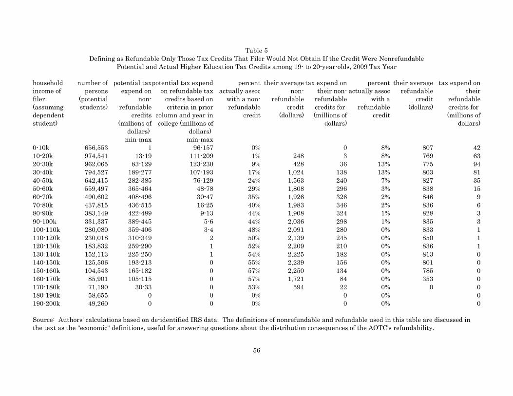
Table 5

Defining as Refundable Only Those Tax Credits That Filer Would Not Obtain If the Credit Were Nonrefundable

Potential and Actual Higher Education Tax Credits among 19- to 20-year-olds, 2009 Tax Year

household

income of

filer

(assuming

dependent

student)

number of

persons

(potential

students)

potential tax

expend on

non-

refundable

credits

(millions of

dollars)

potential tax expend

on refundable tax

credits based on

criteria in prior

column and year in

college (millions of

dollars)

percent

actually assoc

with a non-

refundable

credit

their average

non-

refundable

credit

(dollars)

tax expend on

their non-

refundable

credits for

(millions of

dollars)

percent

actually assoc

with a

refundable

credit

their average

refundable

credit

(dollars)

tax expend on

their

refundable

credits for

(millions of

dollars)

min-max min-max

0-10k 656,553 1 96-157 0% 0 8% 807 42

10-20k 974,541 13-19 111-209 1% 248 3 8% 769 63

20-30k 962,065 83-129 123-230 9% 428 36 13% 775 94

30-40k 794,527 189-277 107-193 17% 1,024 138 13% 803 81

40-50k 642,415 282-385 76-129 24% 1,563 240 7% 827 35

50-60k 559,497 365-464 48-78 29% 1,808 296 3% 838 15

60-70k 490,602 408-496 30-47 35% 1,926 326 2% 846 9

70-80k 437,815 436-515 16-25 40% 1,983 346 2% 836 6

80-90k 383,149 422-489 9-13 44% 1,908 324 1% 828 3

90-100k 331,337 389-445 5-6 44% 2,036 298 1% 835 3

100-110k 280,080 359-406 3-4 48% 2,091 280 0% 833 1

110-120k 230,018 310-349 2 50% 2,139 245 0% 850 1

120-130k 183,832 259-290 1 52% 2,209 210 0% 836 1

130-140k 152,113 225-250 1 54% 2,225 182 0% 813 0

140-150k 125,506 193-213 0 55% 2,239 156 0% 801 0

150-160k 104,543 165-182 0 57% 2,250 134 0% 785 0

160-170k 85,901 105-115 0 57% 1,721 84 0% 353 0

170-180k 71,190 30-33 0 53% 594 22 0% 0 0

180-190k 58,655 0 0 0% 0 0% 0

190-200k 49,260 0 0 0% 0 0% 0

Source: Authors' calculations based on de-identified IRS data. The definitions of nonrefundable and refundable used in this table are discussed in

the text as the "economic" definitions, useful for answering questions about the distribution consequences of the AOTC's refundability.

56

Table 6

Potential and Actual Higher Education Tax Credits among 22- to 23-year-olds, 2008 Tax Year

household income of

filer (assuming

dependent student)

number of persons

(potential students)

percent who appear

to qualify for a non-

refundable credit

based on tuition,

half-time enrollment

(HTC), AGI and tax

liability

potential tax expend

on non-refundable

credits based on

criteria in prior

column and year in

college (millions of

dollars)

percent actually

assoc with a non-

refundable credit

their average non-

refundable credit

(dollars)

tax expend on their

non-refundable

credits for

(millions of dollars)

min-max min-max

0-10k 513,558 1-5% 1 0% 0

10-20k 612,923 5-7% 10-14 1% 218 1

20-30k 680,673 14-17% 48-73 5% 553 18

30-40k 615,158 20-24% 86-131 9% 905 50

40-50k 535,309 25-29% 107-159 12% 1,052 69

50-60k 481,878 29-32% 109-154 12% 1,041 60

60-70k 429,382 28-31% 106-145 13% 1,156 63

70-80k 386,721 32-35% 115-152 15% 1,208 70

80-90k 344,359 37-39% 120-154 17% 1,249 73

90-100k 303,075 41-44% 117-147 17% 1,317 67

100-110k 259,567 44-47% 66-81 11% 941 26

110-120k 200,386 28-30% 9-11 3% 230 1

120-130k 149,979 0% 0 0% 0

130-140k 130,937 0% 0 0% 0

140-150k 108,252 0% 0 0% 0

150-160k 83,317 0% 0 0% 0

160-170k 72,956 0% 0 0% 0

170-180k 61,909 0% 0 0% 0

180-190k 51,640 0% 0 0% 0

190-200k 43,236 0% 0 0% 0

Source: Authors' calculations based on de-identified IRS data.

57

Table 7

Potential and Actual Higher Education Tax Credits among 22- to 23-year-olds, 2009 Tax Year

household

income of

filer

(assuming

dependent

student)

number of

persons

(potential

students)

percent who

appear to

qualify for a

non-

refundable

credit based

on tuition,

AGI and tax

liability

potential tax

expend on non-

refundable

credits based

on criteria in

prior column,

half-time, and

year in college

(millions of

dollars)

percent

who appear

to qualify

for a

refundable

credit

based on

tuition,

AGI and

tax liability

potential tax

expend on

refundable tax

credits based on

criteria in prior

column half-

time and year

in college

(millions of

dollars)

percent

actually

assoc with

a non-

refundable

credit

their

average

non-

refundable

credit

(dollars)

tax expend

on their

non-

refundable

credits for

(millions of

dollars)

percent

actually

assoc with

a

refundable

credit

their

average

refundable

credit

(dollars)

tax expend

on their

refundable

credits for

(millions of

dollars)

min-max min-max min-max min-max

0-10k 517,376 0-1% 1 11-20% 41-85 0% 0 4% 826 18

10-20k 631,684 6-7% 11-15 10-18% 45-93 1% 182 1 6% 792 31

20-30k 680,586 14-18% 51-74 11-20% 54-110 7% 504 24 8% 788 42

30-40k 611,254 22-26% 96-135 13-22% 56-112 12% 885 64 10% 805 49

40-50k 522,568 27-31% 120-163 14-25% 54-108 15% 1,078 85 12% 822 51

50-60k 467,110 31-35% 133-179 15-27% 54-108 17% 1,161 92 14% 843 54

60-70k 415,083 32-37% 132-177 16-30% 52-104 19% 1,232 95 15% 861 54

70-80k 371,824 36-41% 139-180 17-32% 51-101 21% 1,270 99 17% 874 55

80-90k 325,842 40-44% 134-168 18-34% 45-91 23% 1,228 92 19% 830 50

90-100k 281,723 42-45% 126-153 17-33% 39-82 23% 1,316 86 19% 887 47

100-110k 239,392 45-48% 103-134 18-36% 36-74 24% 1,312 77 21% 893 44

110-120k 196,744 47-50% 60-102 19-37% 30-64 24% 1,290 61 22% 899 40

120-130k 155,762 19-38% 36-77 19-38% 24-52 24% 1,351 51 24% 902 34

130-140k 130,193 19-39% 32-68 19-39% 21-45 26% 1,359 45 25% 908 30

140-150k 107,384 20-40% 27-58 20-40% 18-39 27% 1,364 39 26% 910 26

150-160k 89,442 20-41% 23-49 20-41% 15-33 28% 1,369 34 27% 913 22

160-170k 73,893 20-41% 14-31 20-42% 10-21 27% 1,044 21 27% 698 14

170-180k 61,234 20-42% 4-9 20-42% 3-6 24% 364 5 24% 244 4

180-190k 51,035 0% 0 0% 0 0% 0 0% 0

190-200k 42,677 0% 0 0% 0 0% 0 0% 0

Source: Authors' calculations based on de-identified IRS data.

58

Table 8

Defining as Refundable Only Those Tax Credits That Filer Would Not Obtain If the Credit Were Nonrefundable

Potential and Actual Higher Education Tax Credits among 22- to 23-year-olds, 2009 Tax Year

household

income of

filer

(assuming

dependent

student)

number of

persons

(potential

students)

potential tax

expend on

non-

refundable

credits

(millions of

dollars)

potential tax expend

on refundable tax

credits based on

criteria in prior

column and year in

college (millions of

dollars)

percent

actually

assoc with a

non-

refundable

credit

their average

non-

refundable

credit

(dollars)

tax expend on

their non-

refundable

credits for

(millions of

dollars)

percent

actually assoc

with a

refundable

credit

their average

refundable

credit

(dollars)

tax expend on

their

refundable

credits for

(millions of

dollars)

min-max min-max

0-10k 517,376 1 41-85 0% 0 4% 817 18

10-20k 631,684 12-17 44-92 1% 232 2 6% 785 30

20-30k 680,586 58-82 47-102 7% 388 18 9% 791 47

30-40k 611,254 115-164 36-83 12% 876 63 10% 817 50

40-50k 522,568 151-216 22-55 15% 1,478 117 5% 824 20

50-60k 467,110 174-252 13-34 17% 1,699 135 3% 832 11

60-70k 415,083 175-258 9-22 19% 1,835 141 2% 808 8

70-80k 371,824 184-269 5-12 21% 1,917 150 2% 796 5

80-90k 325,842 177-253 2-6 23% 1,861 140 1% 759 3

90-100k 281,723 165-232 1-3 23% 2,010 132 1% 763 1

100-110k 239,392 138-207 0-1 24% 2,068 121 0% 772 0

110-120k 196,744 90-165 0-1 24% 2,128 100 0% 798 0

120-130k 155,762 60-128 0-1 24% 2,242 85 0% 776 0

130-140k 130,193 52-113 0 26% 2,257 75 0% 776 0

140-150k 107,384 45-96 0 27% 2,266 65 0% 782 0

150-160k 89,442 38-81 0 28% 2,275 56 0% 757 0

160-170k 73,893 24-52 0 27% 1,735 35 0% 347 0

170-180k 61,234 7-15 0 24% 615 9 0% 69 0

180-190k 51,035 0 0 0% 0 0% 0

190-200k 42,677 0 0 0% 0 0% 0

Source: Authors' calculations based on de-identified IRS data. The definitions of nonrefundable and refundable used in this table are discussed in

the text as the "economic" definitions, useful for answering questions about the distribution consequences of the AOTC's refundability.

59

Table 9

Potential and Actual Higher Education Tax Credits among 25- to 26-year-olds, 2008 Tax Year

household income of

filer (independent

student)

number of persons

(potential students)

percent who appear

to qualify for a non-

refundable credit

based on tuition,

half-time enrollment

(HTC), AGI and tax

liability

potential tax expend

on non-refundable

credits based on

criteria in prior

column and year in

college (millions of

dollars)

percent actually

assoc with a non-

refundable credit

their average non-

refundable credit

(dollars)

tax expend on their

non-refundable

credits for

(millions of dollars)

min-max min-max

0-10k 513,558 1-5% 1 0% 0

10-20k 612,923 5-7% 10-14 1% 218 1

20-30k 680,673 14-17% 48-73 5% 553 18

30-40k 615,158 20-24% 86-131 9% 905 50

40-50k 535,309 25-29% 107-159 12% 1,052 69

50-60k 481,878 29-32% 109-154 12% 1,041 60

60-70k 429,382 28-31% 106-145 13% 1,156 63

70-80k 386,721 32-35% 115-152 15% 1,208 70

80-90k 344,359 37-39% 120-154 17% 1,249 73

90-100k 303,075 41-44% 117-147 17% 1,317 67

100-110k 259,567 44-47% 66-81 11% 941 26

110-120k 200,386 28-30% 9-11 3% 230 1

120-130k 149,979 0% 0 0% 0

130-140k 130,937 0% 0 0% 0

140-150k 108,252 0% 0 0% 0

150-160k 83,317 0% 0 0% 0

160-170k 72,956 0% 0 0% 0

170-180k 61,909 0% 0 0% 0

180-190k 51,640 0% 0 0% 0

190-200k 43,236 0% 0 0% 0

Source: Authors' calculations based on de-identified IRS data.

60

Table 10

Potential and Actual Higher Education Tax Credits among 25- to 26-year-olds, 2009 Tax Year

household

income of

filer

(independe

nt student)

number of

persons

(potential

students)

percent who

appear to

qualify for a

non-

refundable

credit based

on tuition,

AGI and tax

liability

potential tax

expend on non-

refundable

credits based

on criteria in

prior column,

half-time, and

year in college

(millions of

dollars)

percent

who appear

to qualify

for a

refundable

credit

based on

tuition,

AGI and

tax liability

potential tax

expend on

refundable tax

credits based on

criteria in prior

column half-

time and year

in college

(millions of

dollars)

percent

actually

assoc with

a non-

refundable

credit

their

average

non-

refundable

credit

(dollars)

tax expend

on their

non-

refundable

credits for

(millions of

dollars)

percent

actually

assoc with

a

refundable

credit

their

average

refundable

credit

(dollars)

tax expend

on their

refundable

credits for

(millions of

dollars)

min-max min-max min-max min-max

0-10k 1,783,401 11-12% 116-144 6-10% 81-140 0% 0 7% 806 97

10-20k 1,737,221 12-13% 108-136 4-7% 52-90 11% 464 90 9% 767 115

20-30k 1,487,233 12-13% 122-155 4-6% 40-66 14% 874 179 8% 753 89

30-40k 992,906 13-14% 94-112 4-6% 27-44 14% 931 131 7% 755 53

40-50k 567,754 15-16% 60-71 4-7% 17-29 13% 1,009 74 6% 763 27

50-60k 328,623 16-18% 32-38 5-8% 12-20 10% 986 33 6% 761 15

60-70k 190,235 11-13% 14-19 6-10% 9-15 10% 987 18 6% 766 9

70-80k 111,311 14-17% 11-14 9-13% 7-12 11% 946 11 6% 758 5

80-90k 66,044 18-22% 7-10 12-18% 4-7 11% 879 6 6% 691 3

90-100k 39,555 18-20% 5-6 8-12% 2-4 8% 997 3 4% 762 1

100-110k 24,230 24-26% 3-4 10-16% 2-3 7% 1,008 2 4% 752 1

110-120k 15,245 29-32% 1-2 13-20% 1-2 5% 902 1 4% 761 0

120-130k 9,532 10-14% 1 16-24% 1-2 3% 1,136 0 3% 770 0

130-140k 6,014 12-18% 1 21-31% 1 3% 1,098 0 3% 747 0

140-150k 4,236 14-21% 0-1 23-35% 1 3% 1,126 0 3% 774 0

150-160k 3,233 14-21% 0 25-39% 1 2% 1,111 0 2% 733 0

160-170k 2,253 18-27% 0 29-44% 0-1 3% 891 0 2% 629 0

170-180k 1,577 21-31% 0 33-50% 0 2% 336 0 3% 225 0

180-190k 1,098 0% 0 0% 0 0% 0 0% 0

190-200k 854 0% 0 0% 0 0% 0 0% 0

Source: Authors' calculations based on de-identified IRS data.

61

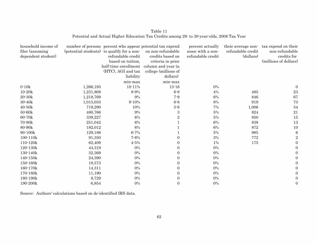
Table 11

Potential and Actual Higher Education Tax Credits among 29- to 30-year-olds, 2008 Tax Year

household income of

filer (assuming

dependent student)

number of persons

(potential students)

percent who appear

to qualify for a non-

refundable credit

based on tuition,

half-time enrollment

(HTC), AGI and tax

liability

potential tax expend

on non-refundable

credits based on

criteria in prior

column and year in

college (millions of

dollars)

percent actually

assoc with a non-

refundable credit

their average non-

refundable credit

(dollars)

tax expend on their

non-refundable

credits for

(millions of dollars)

min-max min-max

0-10k 1,266,193 10-11% 13-16 0% 0

10-20k 1,231,808 8-9% 6-8 4% 485 23

20-30k 1,218,769 9% 7-9 6% 846 67

30-40k 1,015,033 9-10% 6-8 8% 919 73

40-50k 719,290 10% 5-6 7% 1,006 54

50-60k 480,766 9% 3 5% 824 21

60-70k 339,227 6% 2 5% 850 15

70-80k 251,042 6% 1 6% 838 13

80-90k 182,012 6% 1 6% 872 10

90-100k 129,186 6-7% 1 5% 985 6

100-110k 91,350 7-8% 0 3% 772 2

110-120k 62,409 4-5% 0 1% 175 0

120-130k 44,319 0% 0 0% 0

130-140k 32,369 0% 0 0% 0

140-150k 24,390 0% 0 0% 0

150-160k 18,573 0% 0 0% 0

160-170k 14,311 0% 0 0% 0

170-180k 11,190 0% 0 0% 0

180-190k 8,729 0% 0 0% 0

190-200k 6,854 0% 0 0% 0

Source: Authors' calculations based on de-identified IRS data.

62

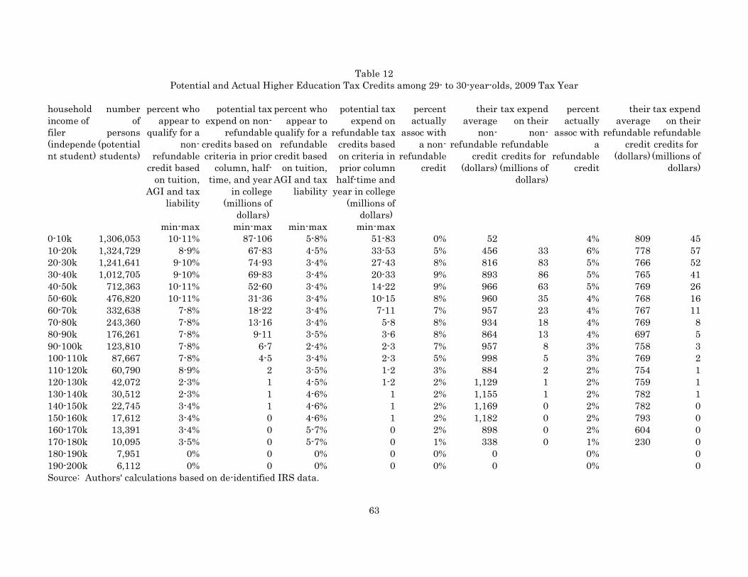
Table 12

Potential and Actual Higher Education Tax Credits among 29- to 30-year-olds, 2009 Tax Year

household

income of

filer

(independe

nt student)

number

of

persons

(potential

students)

percent who

appear to

qualify for a

non-

refundable

credit based

on tuition,

AGI and tax

liability

potential tax

expend on non-

refundable

credits based on

criteria in prior

column, half-

time, and year

in college

(millions of

dollars)

percent who

appear to

qualify for a

refundable

credit based

on tuition,

AGI and tax

liability

potential tax

expend on

refundable tax

credits based

on criteria in

prior column

half-time and

year in college

(millions of

dollars)

percent

actually

assoc with

a non-

refundable

credit

their

average

non-

refundable

credit

(dollars)

tax expend

on their

non-

refundable

credits for

(millions of

dollars)

percent

actually

assoc with

a

refundable

credit

their

average

refundable

credit

(dollars)

tax expend

on their

refundable

credits for

(millions of

dollars)

min-max min-max min-max min-max

0-10k 1,306,053 10-11% 87-106 5-8% 51-83 0% 52 4% 809 45

10-20k 1,324,729 8-9% 67-83 4-5% 33-53 5% 456 33 6% 778 57

20-30k 1,241,641 9-10% 74-93 3-4% 27-43 8% 816 83 5% 766 52

30-40k 1,012,705 9-10% 69-83 3-4% 20-33 9% 893 86 5% 765 41

40-50k 712,363 10-11% 52-60 3-4% 14-22 9% 966 63 5% 769 26

50-60k 476,820 10-11% 31-36 3-4% 10-15 8% 960 35 4% 768 16

60-70k 332,638 7-8% 18-22 3-4% 7-11 7% 957 23 4% 767 11

70-80k 243,360 7-8% 13-16 3-4% 5-8 8% 934 18 4% 769 8

80-90k 176,261 7-8% 9-11 3-5% 3-6 8% 864 13 4% 697 5

90-100k 123,810 7-8% 6-7 2-4% 2-3 7% 957 8 3% 758 3

100-110k 87,667 7-8% 4-5 3-4% 2-3 5% 998 5 3% 769 2

110-120k 60,790 8-9% 2 3-5% 1-2 3% 884 2 2% 754 1

120-130k 42,072 2-3% 1 4-5% 1-2 2% 1,129 1 2% 759 1

130-140k 30,512 2-3% 1 4-6% 1 2% 1,155 1 2% 782 1

140-150k 22,745 3-4% 1 4-6% 1 2% 1,169 0 2% 782 0

150-160k 17,612 3-4% 0 4-6% 1 2% 1,182 0 2% 793 0

160-170k 13,391 3-4% 0 5-7% 0 2% 898 0 2% 604 0

170-180k 10,095 3-5% 0 5-7% 0 1% 338 0 1% 230 0

180-190k 7,951 0% 0 0% 0 0% 0 0% 0

190-200k 6,112 0% 0 0% 0 0% 0 0% 0

Source: Authors' calculations based on de-identified IRS data.

63

Table 13

First Stage of Regression Kink Estimation

Changes in the Slope of the Credit-Income Relationship at the Edges of the Phase-Out Range

coefficient we expect if all students at

lower edge of phase-out qualified for

maximum AOTC (2011) or HTC (2007)

estimated coefficient

dependents of 2011 joint filers lower kink -0.125 -0.1074026***

[<0.001 T]

dependents of 2011 joint filers upper kink 0.125 0.1146557***

[<0.001 T]

dependents of 2011 single filers lower kink -0.250 -0.2019312***

[<0.001 T]

dependents of 2011 single filers upper kink 0.250 0.2164388***

[<0.001 T]

independent 2011 single filers lower kink -0.250 -0.2268326***

[0.001 T]

dependents of 2007 joint filers lower kink -0.090 -0.0731243***

[<0.001 T]

dependents of 2007 joint filers upper kink 0.090 0.0638205***

[<0.001 T]

dependents of 2007 single filers lower kink -0.180 -0.1386706***

[0.001 T]

dependents of 2007 single filers upper kink 0.180 0.1441341***

[0.001 T]

independent 2007 single filers lower kink -0.180 -0.1156229***

[0.001 T]

Source: Authors' estimates based on de-identified IRS data. Robust-to-heteroskedasticity p-values are in square brackets. T indicates that the

estimate passes the Ganong and Jäger (2014) permutation test. The estimates shown are for equations (1) and (4) in the text using cubics for the

polynomials. Households with incomes plus or minus $3,000 around each kink are included.

64

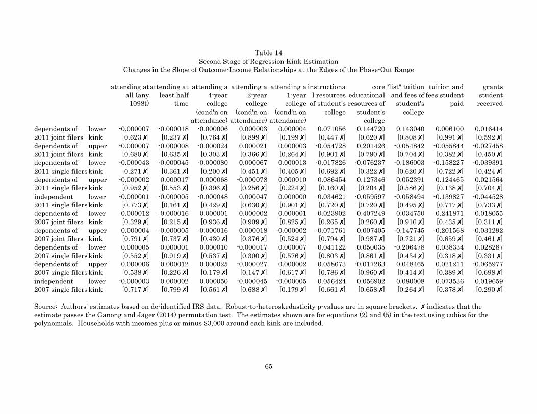
Table 14

Second Stage of Regression Kink Estimation

Changes in the Slope of Outcome-Income Relationships at the Edges of the Phase-Out Range

attending at

all (any

1098t)

attending at

least half

time

attending a

4-year

college

(cond'n on

attendance)

attending a

2-year

college

(cond'n on

attendance)

attending a

1-year

college

(cond'n on

attendance)

instructiona

l resources

of student's

college

core

educational

resources of

student's

college

"list" tuition

and fees of

student's

college

tuition and

fees student

paid

grants

student

received

dependents of

2011 joint filers

lower

kink

-0.000007

[0.623 X]

-0.000018

[0.237 X]

-0.000006

[0.764 X]

0.000003

[0.899 X]

0.000004

[0.199 X]

0.071056

[0.447 X]

0.144720

[0.620 X]

0.143040

[0.808 X]

0.006100

[0.991 X]

0.016414

[0.592 X]

dependents of

2011 joint filers

upper

kink

-0.000007

[0.680 X]

-0.000008

[0.635 X]

-0.000024

[0.303 X]

0.000021

[0.366 X]

0.000003

[0.264 X]

-0.054728

[0.901 X]

0.201426

[0.790 X]

-0.054842

[0.704 X]

-0.055844

[0.382 X]

-0.027458

[0.450 X]

dependents of

2011 single filers

lower

kink

-0.000043

[0.271 X]

-0.000045

[0.361 X]

-0.000080

[0.200 X]

0.000067

[0.451 X]

0.000013

[0.405 X]

-0.017826

[0.692 X]

-0.076237

[0.322 X]

-0.186003

[0.620 X]

-0.158227

[0.722 X]

-0.039391

[0.424 X]

dependents of

2011 single filers

upper

kink

-0.000002

[0.952 X]

0.000017

[0.553 X]

0.000068

[0.396 X]

-0.000078

[0.256 X]

0.000010

[0.224 X]

0.086454

[0.160 X]

0.127346

[0.204 X]

0.052391

[0.586 X]

0.124465

[0.138 X]

0.021564

[0.704 X]

independent

2011 single filers

lower

kink

-0.000001

[0.773 X]

-0.000005

[0.161 X]

-0.000048

[0.429 X]

0.000047

[0.630 X]

0.000000

[0.901 X]

0.034621

[0.720 X]

-0.059597

[0.720 X]

-0.058494

[0.495 X]

-0.139827

[0.717 X]

-0.044528

[0.733 X]

dependents of

2007 joint filers

lower

kink

-0.000012

[0.329 X]

-0.000016

[0.215 X]

0.000001

[0.936 X]

-0.000002

[0.909 X]

0.000001

[0.825 X]

0.023902

[0.265 X]

0.407249

[0.260 X]

-0.034750

[0.916 X]

0.241871

[0.435 X]

0.018055

[0.311 X]

dependents of

2007 joint filers

upper

kink

0.000004

[0.791 X]

-0.000005

[0.737 X]

-0.000016

[0.430 X]

0.000018

[0.376 X]

-0.000002

[0.524 X]

-0.071761

[0.794 X]

0.007405

[0.987 X]

-0.147745

[0.721 X]

-0.201568

[0.659 X]

-0.031292

[0.461 X]

dependents of

2007 single filers

lower

kink

0.000005

[0.552 X]

0.000001

[0.919 X]

0.000010

[0.537 X]

-0.000017

[0.300 X]

0.000007

[0.576 X]

0.041122

[0.803 X]

0.050035

[0.861 X]

-0.206478

[0.434 X]

0.038334

[0.318 X]

0.028287

[0.331 X]

dependents of

2007 single filers

upper

kink

0.000006

[0.538 X]

0.000012

[0.226 X]

0.000025

[0.179 X]

-0.000027

[0.147 X]

0.000002

[0.617 X]

0.058673

[0.786 X]

-0.017263

[0.960 X]

0.048465

[0.414 X]

0.021211

[0.389 X]

-0.065977

[0.698 X]

independent

2007 single filers

lower

kink

-0.000003

[0.717 X]

0.000002

[0.799 X]

0.000050

[0.561 X]

-0.000045

[0.688 X]

-0.000005

[0.179 X]

0.056424

[0.661 X]

0.056902

[0.658 X]

0.080008

[0.264 X]

0.073536

[0.378 X]

0.019659

[0.290 X]

Source: Authors' estimates based on de-identified IRS data. Robust-to-heteroskedasticity p-values are in square brackets. X indicates that the

estimate passes the Ganong and Jäger (2014) permutation test. The estimates shown are for equations (2) and (5) in the text using cubics for the

polynomials. Households with incomes plus or minus $3,000 around each kink are included.

65

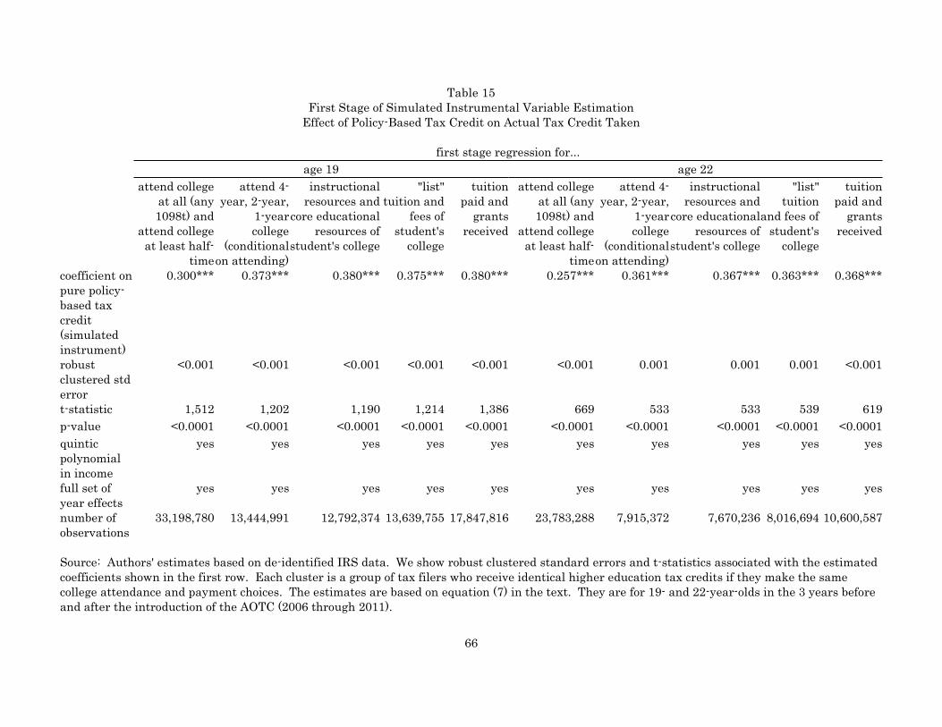
Table 15

First Stage of Simulated Instrumental Variable Estimation

Effect of Policy-Based Tax Credit on Actual Tax Credit Taken

first stage regression for...

age 19 age 22

attend college

at all (any

1098t) and

attend college

at least half-

time

attend 4-

year, 2-year,

1-year

college

(conditional

on attending)

instructional

resources and

core educational

resources of

student's college

"list"

tuition and

fees of

student's

college

tuition

paid and

grants

received

attend college

at all (any

1098t) and

attend college

at least half-

time

attend 4-

year, 2-year,

1-year

college

(conditional

on attending)

instructional

resources and

core educational

resources of

student's college

"list"

tuition

and fees of

student's

college

tuition

paid and

grants

received

coefficient on

pure policy-

based tax

credit

(simulated

instrument)

0.300*** 0.373*** 0.380*** 0.375*** 0.380*** 0.257*** 0.361*** 0.367*** 0.363*** 0.368***

robust

clustered std

error

<0.001 <0.001 <0.001 <0.001 <0.001 <0.001 0.001 0.001 0.001 <0.001

t-statistic 1,512 1,202 1,190 1,214 1,386 669 533 533 539 619

p-value <0.0001 <0.0001 <0.0001 <0.0001 <0.0001 <0.0001 <0.0001 <0.0001 <0.0001 <0.0001

quintic

polynomial

in income

yes yes yes yes yes yes yes yes yes yes

full set of

year effects

yes yes yes yes yes yes yes yes yes yes

number of

observations

33,198,780 13,444,991 12,792,374 13,639,755 17,847,816 23,783,288 7,915,372 7,670,236 8,016,694 10,600,587

Source: Authors' estimates based on de-identified IRS data. We show robust clustered standard errors and t-statistics associated with the estimated

coefficients shown in the first row. Each cluster is a group of tax filers who receive identical higher education tax credits if they make the same

college attendance and payment choices. The estimates are based on equation (7) in the text. They are for 19- and 22-year-olds in the 3 years before

and after the introduction of the AOTC (2006 through 2011).

66

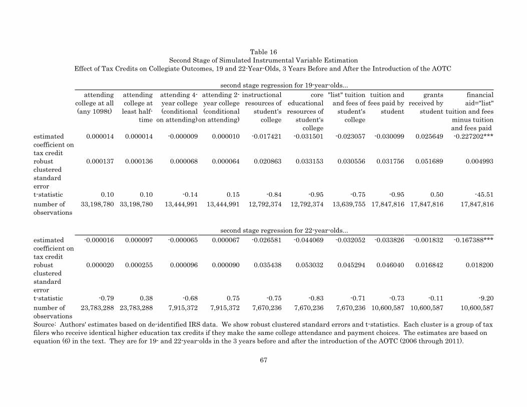
Table 16

Second Stage of Simulated Instrumental Variable Estimation

Effect of Tax Credits on Collegiate Outcomes, 19 and 22-Year-Olds, 3 Years Before and After the Introduction of the AOTC

second stage regression for 19-year-olds...

attending

college at all

(any 1098t)

attending

college at

least half-

time

attending 4-

year college

(conditional

on attending)

attending 2-

year college

(conditional

on attending)

instructional

resources of

student's

college

core

educational

resources of

student's

college

"list" tuition

and fees of

student's

college

tuition and

fees paid by

student

grants

received by

student

financial

aid="list"

tuition and fees

minus tuition

and fees paid

estimated

coefficient on

tax credit

0.000014 0.000014 -0.000009 0.000010 -0.017421 -0.031501 -0.023057 -0.030099 0.025649 -0.227202***

robust

clustered

standard

error

0.000137 0.000136 0.000068 0.000064 0.020863 0.033153 0.030556 0.031756 0.051689 0.004993

t-statistic 0.10 0.10 -0.14 0.15 -0.84 -0.95 -0.75 -0.95 0.50 -45.51

number of

observations

33,198,780 33,198,780 13,444,991 13,444,991 12,792,374 12,792,374 13,639,755 17,847,816 17,847,816 17,847,816

second stage regression for 22-year-olds...

estimated

coefficient on

tax credit

-0.000016 0.000097 -0.000065 0.000067 -0.026581 -0.044069 -0.032052 -0.033826 -0.001832 -0.167388***

robust

clustered

standard

error

0.000020 0.000255 0.000096 0.000090 0.035438 0.053032 0.045294 0.046040 0.016842 0.018200

t-statistic -0.79 0.38 -0.68 0.75 -0.75 -0.83 -0.71 -0.73 -0.11 -9.20

number of

observations

23,783,288 23,783,288 7,915,372 7,915,372 7,670,236 7,670,236 7,670,236 10,600,587 10,600,587 10,600,587

Source: Authors' estimates based on de-identified IRS data. We show robust clustered standard errors and t-statistics. Each cluster is a group of tax

filers who receive identical higher education tax credits if they make the same college attendance and payment choices. The estimates are based on

equation (6) in the text. They are for 19- and 22-year-olds in the 3 years before and after the introduction of the AOTC (2006 through 2011).

67

Appendix Table 1College Assessment Taking and Scores by Household Income

19 and 20 Year Olds in 2008

householdincomecategory

took any college assessment(ACT, SAT, or PSAT)

average math score(SAT scale)

average verbal score(SAT scale)

0-10k 35.0% 458 452

10-20k 35.4% 436 429

20-30k 39.0% 444 437

30-40k 43.1% 457 451

40-50k 47.5% 470 466

50-60k 51.6% 481 476

60-70k 54.6% 489 484

70-80k 58.7% 496 491

80-90k 63.1% 503 497

90-100k 67.6% 510 503

100-110k 72.8% 516 509

110-120k 74.4% 522 514

120-130k 75.9% 527 518

130-140k 80.3% 533 523

140-150k 82.5% 538 528

150-160k 83.3% 542 532

160-170k 85.7% 546 535

170-180k 87.2% 550 539

180-190k 89.9% 553 541

190-200k 89.9% 556 544

Notes: Individuals who were 19 or 20 years old in 2008 are associated with the 2008 income of thefiler of whom they were a dependent at the age of 17. All scores are converted to the SAT© scale.

68

Appendix Table 2

Expenditures on Tax Credits that Coincide More and Less with Third Party Reports, tax filers of all ages in 2011, billions of $2011

using minimum/stringent assumptions on 3rd party reports using maximum/generous assumptions on 3rd party reports

household

income

category

tax expenditures

on credits within

$500 of those

based on third

party reports

tax expenditures

on credits that are

at least $500 more

than those based

on third party

reports

actual and potential tax

expenditures on credits

(including those not taken)

that are at least $500 less

than those based on third

party reports

tax expenditures

on credits within

$500 of those

based on third

party reports

tax expenditures

on credits that are

at least $500 more

than those based

on third party

reports

actual and potential tax

expenditures on credits

(including those not taken)

that are at least $500 less

than those based on third

party reports

0-10k 0.32 0.40 0.68 2.43 0.03 0.17

10-20k 0.54 1.26 1.09 2.96 0.15 0.35

20-30k 0.77 0.77 1.40 2.00 0.16 0.30

30-40k 0.88 0.92 1.81 1.34 0.15 0.25

40-50k 0.75 0.64 1.53 0.87 0.12 0.19

50-60k 0.55 0.56 1.18 0.54 0.08 0.13

60-70k 0.45 0.43 1.00 0.38 0.06 0.10

70-80k 0.45 0.33 0.95 0.31 0.06 0.09

80-90k 0.43 0.61 0.78 0.23 0.05 0.08

90-100k 0.39 0.15 0.61 0.16 0.04 0.06

100-110k 0.31 0.13 0.48 0.13 0.02 0.04

110-120k 0.18 0.06 0.35 0.10 0.01 0.02

120-130k 0.11 0.04 0.27 0.07 0.01 0.01

130-140k 0.10 0.03 0.23 0.06 0.00 0.01

140-150k 0.09 0.05 0.19 0.05 0.00 0.01

150-160k 0.08 0.03 0.17 0.04 0.00 0.01

160-170k 0.05 0.02 0.11 0.03 0.00 0.01

170-180k 0.01 0.14 0.03 0.02 0.00 0.00

180-190k 0.00 0.00 0.00 0.00 0.00 0.00

190-200k 0.00 0.00 0.00 0.00 0.00 0.00

total 6.47 6.43 12.85 7.17 4.92 19.06

Notes: Authors' calculations based on de-identified IRS data. The important third party report for these calculations is Form 1098t.

69