THE RETURN ON INVESTMENT FROMPROPORTIONAL PORTFOLIO STRATEGIES

Sid Browne ∗

Columbia University

Final Version: November 11, 1996

Appeared in: Advances in Applied Probability, 30, 216-238, 1998

Abstract

Dynamic asset allocation strategies that are continuously rebalanced so as to always keepa fixed constant proportion of wealth invested in the various assets at each point in time playa fundamental role in the theory of optimal portfolio strategies. In this paper we study therate of return on investment, defined here as the net gain in wealth divided by the cumulativeinvestment, for such investment strategies in continuous time. Among other results, we provethat the limiting distribution of this measure of return is a gamma distribution. This limit the-orem allows for comparisons of different strategies. For example, the mean return on investmentis maximized by the same strategy that maximizes logarithmic utility, which is also known tomaximize the exponential rate at which wealth grows. The return from this policy turns outto have other stochastic dominance properties as well. We also study the return on the riskyinvestment alone, defined here as the present value of the gain from investment divided by thepresent value of the cumulative investment in the risky asset needed to achieve the gain. Weshow that for the log-optimal, or optimal growth policy, this return tends to an exponentialdistribution. We compare the return from the optimal growth policy with the return from apolicy that invests a constant amount in the risky stock. We show that for the case of a singlerisky investment, the constant investor’s expected return is twice that of the optimal growthpolicy. This difference can be considered the cost for insuring that the proportional investordoes not go bankrupt.

Key words: Portfolio Theory; Diffusions; Stationary Distributions; Convergence in Distribu-tion; Limit Theorems; Stochastic Order Relations; Logarithmic Utility; Optimal Growth Policy.

AMS 1991 Subject Classification: Primary: 90A09, 60F99. Secondary: 90A10, 60J60,60H10.

∗Postal address: 402 Uris Hall, Graduate School of Business, Columbia University, New York, NY 10027 USA.Email:sb30@columbia.edu. Acknowledgment: This paper has benefitted greatly from the very careful reading,corrections and helpful suggestions of an anonymous referee, to whom the author is most grateful.

1 Introduction

Constant proportions investment strategies play a fundamental role in portfolio theory. Under

these policies, an investor follows a dynamic trading strategy that continuously rebalances the

portfolio so as to always allocate fixed constant proportions of the investor’s wealth across the

investment opportunities. These strategies are quite widely used in practice and are also sometimes

referred to as constant mix, or continuously rebalanced, strategies (see e.g., Perold and Sharpe

[25]). Furthermore, for certain objectives and under some specific assumptions about the stochastic

behavior of the investment opportunities, it is well known that these policies have many optimality

properties associated with them as well. These properties are reviewed in the next section.

Given the fundamental nature of such policies in theoretical as well as actual portfolio practice,

it is of interest to know what the stochastic behavior of the rate of return on investment (RROI)

— defined here as the net gain divided by the cumulative investment — is for such policies. In

this paper we study this dimension of the portfolio problem. We take as our setting the continuous

time financial model introduced in Merton [22] and used in Black and Scholes [3]. For this model

we obtain some limit theorems for the RROI which allow us to compare and derive some specific

optimality properties for certain portfolio strategies.

A summary of our main results and the organization of the paper is as follows: in the next sec-

tion, we review the continuous-time model and some well known optimality properties associated

with constant proportion investment policies. In Section 3 we provide our main result (Theo-

rem 3.1): that the return on investment for such policies converges to a limiting distribution which

is a gamma distribution. This result provides a basis upon which to compare different strategies

and to explore and identify various optimality criteria. For example, with this distributional limit

theorem in hand we show in Section 3 that the policy that maximizes logarithmic utility of wealth

generates a RROI that has some stochastic dominance properties over other policies. The logarith-

mic utility function has certain other objective optimality properties that are reviewed in Section 2.

In Section 4 we prove Theorem 3.1. We show in particular that the limiting behavior of the RROI

is in fact determined by the limiting behavior of a related diffusion process, which is completely

analyzed. In Section 5 we move on to consider the excess return from investment above the risk-free

rate. We call this the rate of return on risky investment (RRORI). We show that this measure

converges to a different gamma distribution, and in particular, for the case of logarithmic utility,

to an exponential distribution. However, for the RRORI measure, the logarithmic utility function

has only limited stochastic dominance properties over other policies, and we show that the mean

RRORI is in fact maximized by a different class of strategies, namely, by strategies that invest only

1

a constant amount (as opposed to a constant proportion) in the risky assets. For such strategies the

RRORI follows a Gaussian process that is independent of the constant amount invested in the risky

assets. Furthermore, it turns out that that the mean RRORI for such constant amount investment

strategies is twice the mean RRORI for a logarithmic utility function. (These last two statements

are specific to the case with a single risky stock, and do not hold for the more general case treated in

Section 6.) Since bankruptcy is possible under such strategies, this halved return can be considered

the price the constant proportional investor must pay for the insurance of never going bankrupt,

since in continuous time bankruptcy is impossible under a proportional investment strategy (in the

absence of any withdrawals and other constraints). The precise distributional results obtained in

Section 5 allow us to compute explicitly various comparative probabilities. Finally, in Section 6 we

extend all our results to the multiple risky stock case.

Our study was motivated by the stimulating paper of Ethier and Tavare [9] who studied the

return on investment in a discrete-time gambling model, where the return on the individual gambles

is assumed to follow a random walk. They showed that the asymptotic distribution of the return, as

the mean increment in the random walk goes to zero, is a gamma distribution. Since there is only

one investment opportunity in the model of Ethier and Tavare [9], their results have counterparts in

our treatment of the RRORI, but they did not obtain the discrete-time analogs of our more general

results for the RROI, and hence of the optimality of the logarithmic utility policy, discussed in

Sections 3 and 4.

2 Optimal Properties of Proportional Investment

We recall here some basic facts about certain optimal properties associated with investment policies

that invest a fixed proportion (possibly greater than 1) of current wealth in the risky asset. These

policies are commonly referred to as constant proportions or constant mix strategies. While for

expositional purposes we concentrate on the case of a single stock in Sections 3-5, we introduce

here the model with an arbitrary number of risky stocks since we will return to the multiple stock

case later in Section 6.

The model we treat is that of a complete market with constant coefficients, with k (correlated)

risky stocks generated by k independent Brownian motions. The prices of these stocks will be

denoted by {S(i)t : i = 1, . . . , k}, where it is assumed that the prices evolve according to

dS(i)t = µiS

(i)t dt+

k∑j=1

σijS(i)t dW

(j)t , for i = 1, . . . , k (2.1)

where {µi : i = 1, . . . , k} and {σij : i, j = 1, . . . , k} are constants, and W(j)t denotes a standard

2

independent Brownian motion, for j = 1, . . . , k. There is also a risk-free security, a bond, available

for investment. The price of the bond, {Bt, t ≥ 0}, evolves according to

dBt = rBtdt , (2.2)

where r > 0 is a constant. Thus the stock prices follow a multi-dimensional geometric Brownian

motion, as introduced in Merton [22].

An investment policy is a (column) vector control process {πt : t ≥ 0} with individual compo-

nents πi(t), i = 1, . . . , k, where πi(t) is the proportion of the investor’s wealth invested in the risky

asset i at time t, for i = 1, . . . , k, with the remainder invested in the risk-free bond. Thus, under

the policy π, the investor’s wealth process, Xπt evolves according to

dXπt = Xπ

t

(k∑i=1

πi(t)dS

(i)t

S(i)t

)+Xπ

t

k∑i=1

(1− πi(t))dBtBt

= Xπt

(r + π

′t(µ− r1)

)dt+Xπ

t

k∑i=1

k∑j=1

πi(t)σij dW(j)t , (2.3)

upon substitution from (2.1) and (2.2), where πt = (π1(t), . . . , πk(t))′, µ = (µ1, . . . , µk)

′, and

1 = (1, . . . , 1)′

(transposition is denoted by the superscript′). It is of course assumed that πt is an

admissible control process, i.e., it is a nonanticipative adapted vector satisfying∫ T0 π

′tπtdt < ∞,

for all T < ∞. We place no further restrictions on π. For example we allow πi(t) < 0, in which

case the investor is selling the ith stock short, as well as πi(t) > 1, for any and all i = 1, . . . , k.

Let σ denote the matrix σ = (σ)ij , and let Σ = σσ′. We will assume for the remainder that

the matrix σ is of full rank, and hence σ−1 as well as Σ−1 exist.

For the sequel, let

µ̃ := µ− r1 (2.4)

denote the vector of the excess returns of the risky stocks over the risk-free return.

2.1 Optimality of constant proportions

Of particular interest to us is the case where πt is a constant vector for all t ≥ 0. Such a policy

is called a constant proportions policy and is in fact the optimal investment policy for many

interesting objective functions. For example, it is well known that if the investor’s objective is

to choose an admissible investment strategy to maximize expected utility of terminal wealth for a

utility function that is either a power function, or logarithmic, then the optimal policy is a constant

vector. Furthermore, a constant vector is also the optimal policy for other objective criteria, such

as minimizing the expected time to reach a given level of wealth, as well. We summarize these

main properties in the following:

3

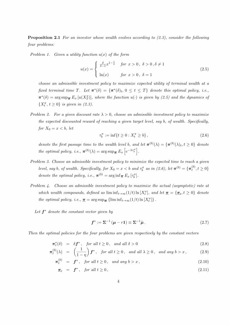
Proposition 2.1 For an investor whose wealth evolves according to (2.3), consider the following

four problems:

Problem 1. Given a utility function u(x) of the form

u(x) =

δδ−1x

1− 1δ for x > 0 , δ > 0 , δ 6= 1

ln(x) for x > 0 , δ = 1

(2.5)

choose an admissible investment policy to maximize expected utility of terminal wealth at a

fixed terminal time T . Let π∗(δ) = {π∗(δ)t, 0 ≤ t ≤ T} denote this optimal policy, i.e.,

π∗(δ) = arg supπ Ex [u(XπT )], where the function u(·) is given by (2.5) and the dynamics of

{Xπt , t ≥ 0} is given in (2.3).

Problem 2. For a given discount rate λ > 0, choose an admissible investment policy to maximize

the expected discounted reward of reaching a given target level, say b, of wealth. Specifically,

for X0 = x < b, let

τπb := inf{t ≥ 0 : Xπt ≥ b} , (2.6)

denote the first passage time to the wealth level b, and let π(b)(λ) = {π(b)(λ)t, t ≥ 0} denote

the optimal policy, i.e., π(b)(λ) = arg supπ Ex[e−λτ

πb

].

Problem 3. Choose an admissible investment policy to minimize the expected time to reach a given

level, say b, of wealth. Specifically, for X0 = x < b and τπb as in (2.6), let π(b) = {π(b)t , t ≥ 0}

denote the optimal policy, i.e., π(b) = arg infπ Ex [τπb ].

Problem 4. Choose an admissible investment policy to maximize the actual (asymptotic) rate at

which wealth compounds, defined as lim inft→∞(1/t) ln [Xπt ], and let π = {πt, t ≥ 0} denote

the optimal policy, i.e., π = arg supπ {lim inft→∞(1/t) ln [Xπt ]} .

Let f∗ denote the constant vector given by

f∗ := Σ−1 (µ− r1) ≡ Σ−1µ̃ . (2.7)

Then the optimal policies for the four problems are given respectively by the constant vectors

π∗t (δ) = δf∗ , for all t ≥ 0 , and all δ > 0 (2.8)

π(b)t (λ) =

(1

1− η

)f∗ , for all t ≥ 0 , and all λ ≥ 0 , and any b > x , (2.9)

π(b)t = f∗ , for all t ≥ 0 , and any b > x , (2.10)

πt = f∗ , for all t ≥ 0 , (2.11)

4

where in (2.9), η = η(λ) satisfies 0 < η < 1 and is the (smaller) root to the quadratic equation

η2r − η(γ + λ+ r) + λ = 0, where the parameter γ := (1/2)µ̃′Σ−1µ̃.

Problem 1 and its optimal policy (2.8) were first considered in Merton [22]. The identical policy is

in effect if the investor maximizes utility obtained from consumption as well (see Merton [22, 23]

for more details). Problem 2 and its optimal policy (2.9) follows from a somewhat more general

result of Browne [6, Theorem 4.3] (see also Orey et al.[24]). Problem 3 and its optimal policy (2.10)

was first considered in Heath et al.[15] for the case k = 1 (see also Merton[23, Section 6.5]). The

multivariate case follows directly from the more general result in Browne [6]. It is interesting to

note that the optimal policies for Problems 2 and 3 are independent of the target level of wealth b.

Problem 4 was considered in Karatzas [17, Section 9.6].

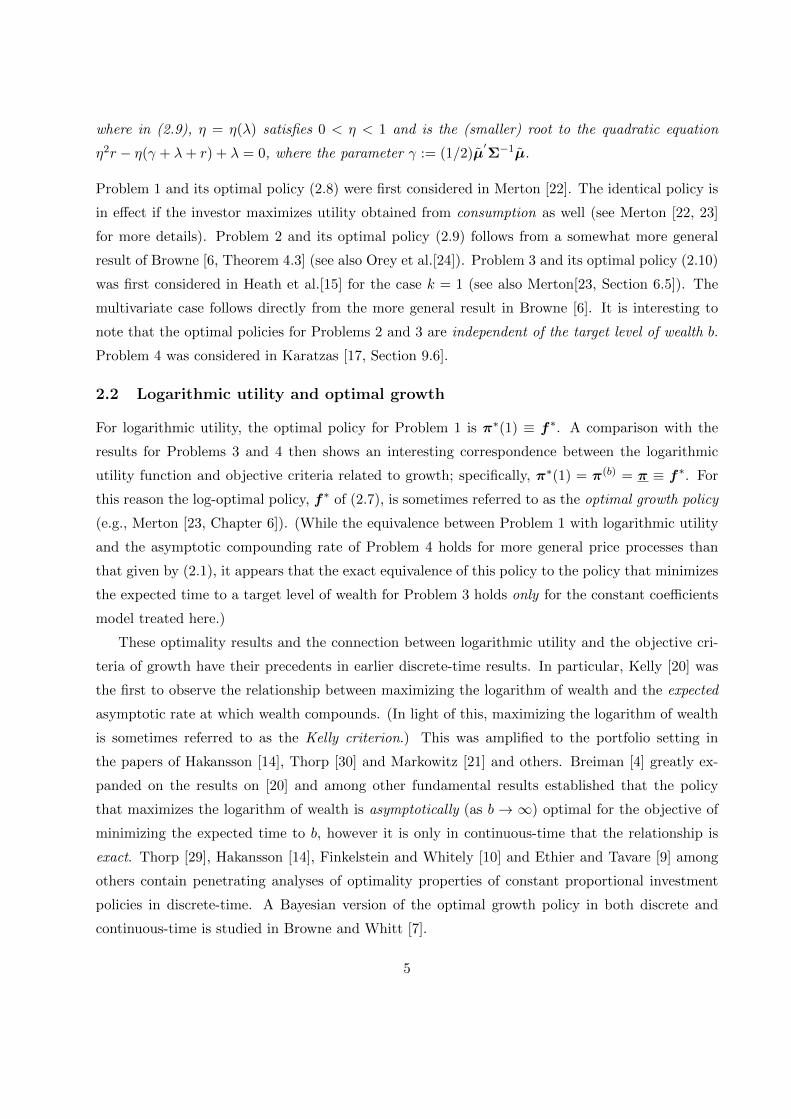
2.2 Logarithmic utility and optimal growth

For logarithmic utility, the optimal policy for Problem 1 is π∗(1) ≡ f∗. A comparison with the

results for Problems 3 and 4 then shows an interesting correspondence between the logarithmic

utility function and objective criteria related to growth; specifically, π∗(1) = π(b) = π ≡ f∗. For

this reason the log-optimal policy, f∗ of (2.7), is sometimes referred to as the optimal growth policy

(e.g., Merton [23, Chapter 6]). (While the equivalence between Problem 1 with logarithmic utility

and the asymptotic compounding rate of Problem 4 holds for more general price processes than

that given by (2.1), it appears that the exact equivalence of this policy to the policy that minimizes

the expected time to a target level of wealth for Problem 3 holds only for the constant coefficients

model treated here.)

These optimality results and the connection between logarithmic utility and the objective cri-

teria of growth have their precedents in earlier discrete-time results. In particular, Kelly [20] was

the first to observe the relationship between maximizing the logarithm of wealth and the expected

asymptotic rate at which wealth compounds. (In light of this, maximizing the logarithm of wealth

is sometimes referred to as the Kelly criterion.) This was amplified to the portfolio setting in

the papers of Hakansson [14], Thorp [30] and Markowitz [21] and others. Breiman [4] greatly ex-

panded on the results on [20] and among other fundamental results established that the policy

that maximizes the logarithm of wealth is asymptotically (as b → ∞) optimal for the objective of

minimizing the expected time to b, however it is only in continuous-time that the relationship is

exact. Thorp [29], Hakansson [14], Finkelstein and Whitely [10] and Ethier and Tavare [9] among

others contain penetrating analyses of optimality properties of constant proportional investment

policies in discrete-time. A Bayesian version of the optimal growth policy in both discrete and

continuous-time is studied in Browne and Whitt [7].

5

A comparison of (2.9) with (2.5) and (2.8) shows that just as the logarithmic utility function

is related to optimal growth, a power utility function with δ 6= 1 is also related to certain growth

objectives related to that of Problem 2 (in particular for δ = (1 − η)−1 in (2.5)). (Relationships

between objective criteria other than growth and particular utility functions for some other portfolio

problems are discussed in Browne [5].)

Remark 2.1: Risk aversion. The Arrow-Pratt measure of relative risk aversion for a utility

function u(·), denoted here by Λ(·), is defined as Λ(x) := −xu(2)(x)/u(1)(x), where u(i)(x) :=diu(x)dxi

, see [26]. Thus for the power utility function in (2.5) we have Λ(x) = δ−1 for all x > 0,

corresponding to constant relative risk aversion. Since the logarithmic case corresponds to

a relative risk aversion Λ(x) = 1, it is seen from (2.8) that for the case where f∗′1 > 0, an

investor who is more risk averse than a logarithmic investor (i.e., δ < 1) will in fact under-

invest in the risky assets relative to the logarithmic investor while an investor who is less risk

averse (δ > 1) will over-invest in the risky assets relative to the logarithmic investor.

Since constant proportion investment policies play such a fundamental role in portfolio theory, and

is the focus of study here, we summarize its main properties next. For models where the optimal

policy is a constant proportion of the surplus of wealth over some level — instead of wealth itself

— see Gottlieb [11], Sundaresan[27], Black and Perold[2], Grossman and Zhou[13], Dybvig[8] and

Browne[6].

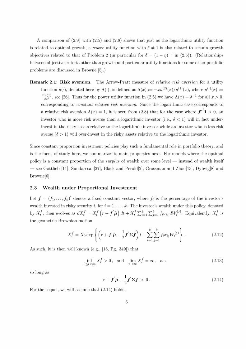
2.3 Wealth under Proportional Investment

Let f = (f1, . . . , fk)′

denote a fixed constant vector, where fi is the percentage of the investor’s

wealth invested in risky security i, for i = 1, . . . , k. The investor’s wealth under this policy, denoted

by Xft , then evolves as dXf

t = Xft

(r + f

′µ̃)dt + Xf

t

∑ki=1

∑kj=1 fiσij dW

(j)t . Equivalently, Xf

t is

the geometric Brownian motion

Xft = X0 exp

(r + f

′µ̃− 1

2f′Σf

)t+

k∑i=1

k∑j=1

fiσijW(j)t

. (2.12)

As such, it is then well known (e.g., [18, Pg. 349]) that

inf0≤t<∞

Xft > 0 , and lim

t→∞Xft =∞ , a.s. (2.13)

so long as

r + f′µ̃− 1

2f′Σf > 0 . (2.14)

For the sequel, we will assume that (2.14) holds.

6

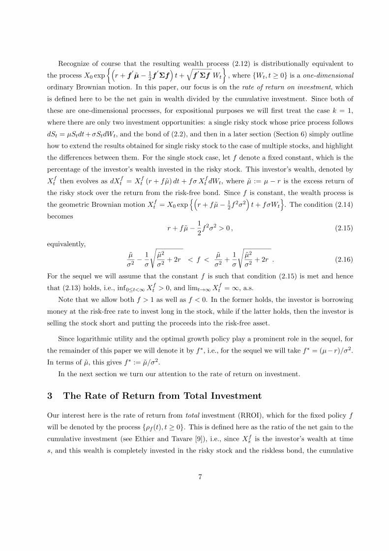
Recognize of course that the resulting wealth process (2.12) is distributionally equivalent to

the process X0 exp

{(r + f

′µ̃− 1

2f′Σf

)t+

√f′Σf Wt

}, where {Wt, t ≥ 0} is a one-dimensional

ordinary Brownian motion. In this paper, our focus is on the rate of return on investment, which

is defined here to be the net gain in wealth divided by the cumulative investment. Since both of

these are one-dimensional processes, for expositional purposes we will first treat the case k = 1,

where there are only two investment opportunities: a single risky stock whose price process follows

dSt = µStdt+σStdWt, and the bond of (2.2), and then in a later section (Section 6) simply outline

how to extend the results obtained for single risky stock to the case of multiple stocks, and highlight

the differences between them. For the single stock case, let f denote a fixed constant, which is the

percentage of the investor’s wealth invested in the risky stock. This investor’s wealth, denoted by

Xft then evolves as dXf

t = Xft (r + fµ̃) dt + fσXf

t dWt, where µ̃ := µ − r is the excess return of

the risky stock over the return from the risk-free bond. Since f is constant, the wealth process is

the geometric Brownian motion Xft = X0 exp

{(r + fµ̃− 1

2f2σ2

)t+ fσWt

}. The condition (2.14)

becomes

r + fµ̃− 1

2f2σ2 > 0 , (2.15)

equivalently,

µ̃

σ2− 1

σ

√µ̃2

σ2+ 2r < f <

µ̃

σ2+

1

σ

√µ̃2

σ2+ 2r . (2.16)

For the sequel we will assume that the constant f is such that condition (2.15) is met and hence

that (2.13) holds, i.e., inf0≤t<∞Xft > 0, and limt→∞X

ft =∞, a.s.

Note that we allow both f > 1 as well as f < 0. In the former holds, the investor is borrowing

money at the risk-free rate to invest long in the stock, while if the latter holds, then the investor is

selling the stock short and putting the proceeds into the risk-free asset.

Since logarithmic utility and the optimal growth policy play a prominent role in the sequel, for

the remainder of this paper we will denote it by f∗, i.e., for the sequel we will take f∗ = (µ−r)/σ2.In terms of µ̃, this gives f∗ := µ̃/σ2.

In the next section we turn our attention to the rate of return on investment.

3 The Rate of Return from Total Investment

Our interest here is the rate of return from total investment (RROI), which for the fixed policy f

will be denoted by the process {ρf (t), t ≥ 0}. This is defined here as the ratio of the net gain to the

cumulative investment (see Ethier and Tavare [9]), i.e., since Xfs is the investor’s wealth at time

s, and this wealth is completely invested in the risky stock and the riskless bond, the cumulative

7

investment until time t is then∫ t0 X

fs ds, and the RROI is then defined by

ρf (t) :=Xft −X0∫ t0 X

fs ds

, for t > 0 . (3.1)

Thus ρf (t) is a measure of the amount of wealth it takes to finance a gain. If ρf (t) is large,

then the investor is accumulating gains at a faster rate than if it is small (see Remark 3.1 below

for a discussion of other measures of rate of return). Note that if we divide the numerator and

denominator of the ratio in (3.1) by t, we may also interpret the measure ρf (t) as the average net

gain over the average wealth level.

Substitution of (2.3) into (3.1) shows that for a fixed f ,

ρf (t) =exp

{(r + fµ̃− 1

2f2σ2

)t+ fσWt

}− 1∫ t

0 exp{(r + fµ̃− 1

2f2σ2

)s+ fσWs

}ds. (3.2)

Placing f = 0 in (3.2) shows that for that policy, under which total wealth is always invested in

the risk-free asset, we do have

ρ0(t) :=ert − 1∫ t0 e

rsds= r

the risk-free interest rate, as expected. However, for f 6= 0, the RROI process {ρf (t), t > 0} is

quite complicated and does not yield to a simple direct analysis. Nevertheless, we will show that for

any fixed proportion f such that (2.15) holds, the process {ρf (t), t > 0} admits a unique limiting

distribution, which is a gamma distribution. We make this more precise in the next theorem.

Remark on notation: For reference, we note that throughout the remainder of the paper, when

we say that a random variable X ∼ gamma(α, β), we mean that X is a random variable with

density function ψ(x) = e−βxxα−1βα/Γ(α), and so E(X) = α/β, and V ar(X) = α/β2.

Our main result can now be stated as the following:

Theorem 3.1 For any fixed proportional strategy f which satisfies condition (2.15), the RROI

process {ρf (t), t > 0} converges (as t → ∞) in distribution to a random variable which has a

gamma distribution. Specifically, as t→∞,

ρf (t)d−→ ρf ∼ gamma

(2 (r + fµ̃)

σ2f2− 1 ,

2

σ2f2

), (3.3)

whered−→ denotes convergence in distribution. As such

E[ρf ] = r + fµ̃− 1

2f2σ2 > 0 . (3.4)

8

The proof of this theorem is given in the next section. However, since the precise distributional

nature of the result allows us a basis upon which to compare different investment strategies, we

will investigate some of its ramifications directly.

Remark 3.1: Our definition of ρf (t) as the rate of return on investment, while based directly on

measures studied in Ethier and Tavare [9] (see also Griffin [12]), is not quite the rate of return

that is typically used in corporate finance. In continuous-time the rate of return until time t

from the portfolio strategy f is more usually defined in the financial literature as the value

of rf (t) such that X0erf (t) t = Xf

t . (Recall that in discrete time, if an investment yields a

return ri in period i, then an initial investment of X0 grows (if all gains are reinvested) after

n investment periods to Xn = X0∏ni=1(1 + ri). The rate of return is then typically defined as

that value of r∗n such that [(1 + r∗n)n − 1] = [Xn −X0] /X0, from which it follows that r∗n =

[∏ni=1(1 + ri)]

1/n−1. It should be clear that the analog of this for our continuous-time model

with continuous reinvestment is indeed rf (t). The rate of return measure studied by Ethier

and Tavare [9] is defined in discrete-time by Rn := [Xn −X0] /∑n−1i=0 Xi, the continuous-time

analog of which is clearly our ρf (t).)

Using (2.12), it is seen that rf (t) = r+fµ̃− 12f

2σ2 + 1t fσWt, and so for any t > 0, E[rf (t)] =

r + fµ̃ − f2σ2/2, which by (3.4) is equivalent to E[ρf ]. However, the measure rf (t) has a

degenerate stochastic limit, since by the law of large numbers rf (t)a.s.−→ r + fµ̃ − f2σ2/2 ≡

E[ρf ], as t→∞. Thus the more usual measure rf (t) does not convey any information about

the variation of the asymptotic return around the mean. By Theorem 3.1 above, we see that

such (more refined) information is indeed provided by the measure ρf .

Remark 3.2: The expectation in (3.4) should not be confused with the ratio of the expected gain

to the expected total investment, which for any t > 0, is equal to

E[total gain]

E[total investment]≡E[Xft −X0

]E[∫ t

0 Xfs ds

] = r + fµ̃ . (3.5)

(This can be established by recognizing that EXft = X0e

(r+fµ̃)t, and then by using Fubini’s

theorem to compute the expectation in the denominator.)

The distinction between measures related to (3.4) and (3.5) for simple discrete-time gambling

models is discussed in Griffin [12].

9

3.1 Optimal Growth Policy and Stochastic Dominance

Note that while r+fµ̃ is unbounded in f , hence implying that the quantity in (3.5) is maximized by

a strategy that invests as much as possible in the risky asset, the mean RROI of (3.4), r+fµ̃− 12f

2σ2,

is maximized at a finite value. In particular at the value f∗ = µ̃/σ2, which is the same policy that

is optimal for maximizing logarithmic utility of wealth at a fixed terminal time and hence for

maximizing the asymptotic (exponential) rate of growth, and by the results of [15, 23, 6] is also

optimal for minimizing the expected time to a goal, i.e., the mean RROI is maximized by the

log-optimal or ordinary optimal-growth strategy of (2.7). Thus, we find that a byproduct of our

analysis is that it provides yet another objective justification for the use of logarithmic utility. We

make this precise in the following.

Corollary 3.2 The mean of the limiting distribution of the RROI process is maximized at the value

f∗ =µ̃

σ2, (3.6)

with resulting mean E[ρ∗] = r+γ, where γ := 12 (µ̃/σ)2. For this strategy the RROI, ρ∗(t), satisfies

ρ∗(t)d−→ ρ∗ ∼ gamma

(r + γ

γ,

1

γ

). (3.7)

In fact, the precise distributional characterization of the limiting RROI allows for a somewhat

stronger statement, in terms of stochastic orderings. Recall first (see e.g. Stoyan [28]) that for

two random variables, X,Y , we say that X ≤icx Y if E(X − x)+ ≤ E(Y − x)+ for all x. This is

equivalent to saying that E[g(X)] ≤ E[g(Y )] for all increasing convex functions g, and is referred

to as the increasing convex ordering. We also say that X ≤icv Y if E(x −X)+ ≥ E(x − Y )+, for

all x (provided the expectations are finite). This is equivalent to saying that E[h(X)] ≤ E[h(Y )]

for all increasing concave functions h, and is hence referred to as the increasing concave ordering.

(This last ordering is also referred to as second degree stochastic monotonic dominance (see [16,

Section 2.9]).)

The following corollary shows that the RROI obtained from using the optimal growth policy

dominates in the increasing convex stochastic order the RROI from any other proportional strategy

that under-invests relative to it, and dominates in the increasing concave stochastic order the RROI

for any proportional strategy that over-invests relative to it.

Corollary 3.3 Let ρ∗ denote the RROI obtained from using the policy f∗ defined in (3.6), and let

ρf be the RROI from any other constant proportional strategy f := cf∗, where c is an arbitrary

constant. Then the following hold:

ρf ≤icx ρ∗ for c ≤ 1, (3.8)

10

ρf ≤icv ρ∗ for c ≥ 1. (3.9)

Proof: See Appendix A.1.

Comparing Corollary 3.3 with equations (2.5) and (2.8), and the earlier discussion of risk aver-

sion in Remark 2.1, shows clearly that (3.8) is in effect for an investor with greater relative risk

aversion than a log investor, while (3.9) is in effect for an investor with less relative risk aversion.

Remark 3.3: It should be noted that while the previous two corollaries highlight some optimal

properties of the log-optimal strategy, it is not claimed that the log-optimal strategy, f∗, is

in fact the strategy that maximizes the mean RROI over all admissible strategies — only

among all constant proportional ones. It is an open question as to what the actual (global)

optimal strategy is for this criterion.

Remark 3.4: It is interesting to observe that we cannot extend Corollary 3.3 to get a standard

stronger stochastic ordering in general with respect to over or under investing relative to

the log-optimal policy. Rather, we can only obtain a (sharp) characterization of the type of

constant proportional strategies that yield RROIs that are stochastically dominated by the

RROI from the log-optimal or optimal growth policy. However, before we proceed we recall

the likelihood ratio order, denoted by ≤LR. This stochastic order is stronger than (and hence

implies) the stochastic order ≤st, which is also known as “first degree stochastic dominance”

(see [16]). (Recall that X ≤st Y if P (X ≥ z) ≤ P (Y ≥ z), for all z.)

For two continuous nonnegative random variables, X1, X2, with densities ψ1(x) and ψ2(x),

we say that X2 ≤LR X1 if

ψ1(y)

ψ1(x)≥ ψ2(y)

ψ2(x)for all x ≤ y . (3.10)

Corollary 3.4 For a proportional strategy f = cf∗, with c 6= 1, where f∗ is the optimal

policy of (3.6), the relationship ρf ≤LR ρ∗ (which implies the weaker relationship ρf ≤st ρ∗)

holds if and only if c satisfies

1−√r + γ

γ< c < − r

r + 2γ. (3.11)

Proof: See Appendix A.2.

Corollary 3.4 shows that the only type of constant proportional policy (other than f∗) for

which the RROI is stochastically dominated by the optimal growth policy is one that is

shorting the stock to the degree required by (3.11).

11

4 Proof of Theorem 3.1 and a Related Diffusion Process

In this section we provide the proof of Theorem 3.1. While the process {ρf (t), t ≥ 0} does not

admit a simple direct analysis, there is a related Markov process amenable to analysis which holds

the key for the limiting behavior of {ρf (t)}. Specifically, the process {Rf (t), t ≥ 0} defined by

Rf (t) :=Xft

X0 +∫ t0 X

fs ds

. (4.1)

(Note that Rf (0) = 1.) We will first show that the limiting behavior of {ρf (t)} is equivalent to

the limiting behavior of the process {Rf (t)}. Since our main interest here is in fact on the limiting

behavior of the RROI process {ρf (t)}, this is quite convenient, since as we will show below {Rf (t)}is in fact a diffusion process whose limiting behavior we can analyze precisely.

Theorem 4.1 Suppose that for some random variable Rf , we have Rf (t)d−→ Rf as t→∞. Then

for any f that satisfies (2.15) we have, as t→∞,

ρf (t)d−→ Rf . (4.2)

Proof: Observe that

ρf (t) = Rf (t)

[Xft −X0

Xft

] [X0 +

∫ t0 X

fs ds∫ t

0 Xfs ds

]≡ Rf (t)

[1− e−Bt

] [1 +

1∫ t0 e

Bsds

](4.3)

where {Bs, s ≥ 0} is the linear Brownian motion defined by

Bs :=

(r + fµ̃− f2σ2

2

)s+ fσWs , with B0 = 0.

If (2.15) holds, then {Bs} has positive drift, which then implies that limt→∞ e−Bt = 0 a.s.,

as well as limt→∞(∫ t

0 eBsds

)−1= 0 a.s., which in turn implies the distributional limit (4.2) as a

consequence of Theorem 4.4 of Billingsley [1].

As such, Theorem 3.1 will be completely established if we can now prove that Rf (t)d−→ Rf ,

for some random variable Rf with Rf = ρf , i.e., we must establish that {Rf (t)} has the limiting

gamma distribution posited earlier. To that end, we will first show that the process {Rf (t)} is

in fact a temporally homogeneous diffusion. This enables us to use standard techniques from the

theory of diffusion processes to establish its limiting stationary distribution exactly. We will also

prove that {Rf (t)} is uniformly integrable. We begin by first noting the following.

Proposition 4.2 For a fixed proportional investment policy f , the process {Rf (t)} follows the

stochastic differential equation

dRf (t) =[(r + fµ̃)Rf (t)−R2

f (t)]dt+ fσRf (t)dWt , (4.4)

12

i.e., {Rf (t)} is a temporally homogeneous diffusion process with drift function b(x) = (r+fµ̃)x−x2

and diffusion function v2(x) = f2σ2x2.

Proof: Defining At :=∫ t0 X

fs ds as the cumulative wealth (investment) process, we may write

Rf (t) = Xft /(X0 + At). Since At is a process of bounded first variation, its quadratic variation is

zero, and so Ito’s rule shows that dAt = Xft dt. Applying Ito’s rule to Xf

t /(X0 +At) gives

dXft

X0 +At=

1

X0 +AtdXf

t −Xft

(X0 +At)2dAt

which upon substitution gives

dXft

X0 +At=

Xft

X0 +At(r + fµ̃)dt+

Xft

X0 +AtfσdWt −

(Xft

X0 +At

)2

dt

which is equivalent to (4.4).

The fact that the {Rf (t)} follows the stochastic differential equation (4.4) allows us to conclude

that it is in fact a strongly ergodic Markov process with a gamma stationary distribution. We state

this as a theorem next. The proof will follow as an application of the more general lemma that

follows directly.

Theorem 4.3

Rf (t)d−→ Rf ∼ gamma

(2 (r + fµ̃)

σ2f2− 1 ,

2

σ2f2

). (4.5)

Moreover the the process Rf (t) is uniformly integrable, and hence

limt→∞

E(Rf (t)) = E[Rf ] = r + fµ̃− 1

2f2σ2 . (4.6)

Proof: Since we will have other occasions to examine stochastic differential equations similar

to (4.4), we will establish the result for the more general stochastic differential equation dZt =[aZt − bZ2

t

]dt + cZtdWt, of which (4.4) is just a special case with a = r + fµ̃, b = 1, c = fσ.

Therefore, Theorem 4.3 (and then in light of Theorem 4.1, by implication Theorem 3.1) is just a

consequence of the following lemma:

Lemma 4.4 Suppose Zt evolves as the stochastic differential equation

dZt =[aZt − bZ2

t

]dt+ cZtdWt (4.7)

with a > 0, b > 0. Then

(i)

Zt =Z0 exp

{(a− 1

2c2)t+ cWt

}1 + Z0 b

∫ t0 exp

{(a− 1

2c2)s+ cWs

}ds. (4.8)

13

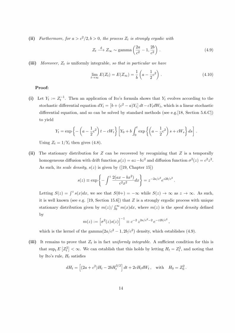
(ii) Furthermore, for a > c2/2, b > 0, the process Zt is strongly ergodic with

Ztd−→ Z∞ ∼ gamma

(2a

c2− 1,

2b

c2

). (4.9)

(iii) Moreover, Zt is uniformly integrable, so that in particular we have

limt→∞

E(Zt) = E(Z∞) =1

b

(a− 1

2c2). (4.10)

Proof:

(i) Let Yt := Z−1t . Then an application of Ito’s formula shows that Yt evolves according to the

stochastic differential equation dYt =[b+ (c2 − a)Yt

]dt−cYtdWt, which is a linear stochastic

differential equation, and so can be solved by standard methods (see e.g.[18, Section 5.6.C])

to yield

Yt = exp

{−(a− 1

2c2)t− cWt

}[Y0 + b

∫ t

0exp

{(a− 1

2c2)s+ cWs

}ds

].

Using Zt = 1/Yt then gives (4.8).

(ii) The stationary distribution for Z can be recovered by recognizing that Z is a temporally

homogeneous diffusion with drift function µ(z) = az−bz2 and diffusion function σ2(z) = c2z2.

As such, its scale density, s(z) is given by ([19, Chapter 15])

s(z) ≡ exp

{−∫ z 2(ax− bx2)

c2x2dx

}= z−2a/c

2ez2b/c

2.

Letting S(z) =∫ z s(x)dx, we see that S(0+) = −∞ while S(z) → ∞ as z → ∞. As such,

it is well known (see e.g. [19, Section 15.6]) that Z is a strongly ergodic process with unique

stationary distribution given by m(z)/∫∞0 m(x)dx, where m(z) is the speed density defined

by

m(z) :=[σ2(z)s(z)

]−1≡ c−2 z2a/c2−2 e−z2b/c2 ,

which is the kernel of the gamma(2a/c2 − 1, 2b/c2

)density, which establishes (4.9).

(iii) It remains to prove that Zt is in fact uniformly integrable. A sufficient condition for this is

that suptE[Z2t

]<∞. We can establish that this holds by letting Ht = Z2

t , and noting that

by Ito’s rule, Ht satisfies

dHt =[(2a+ c2)Ht − 2bH

3/2t

]dt+ 2cHtdWt , with H0 = Z2

0 .

14

Since b > 0, we may now choose constants α > 0 and β > 0 so that

α− βx > (2a+ c2)x− 2bx3/2 , for x ≥ 0 ,

and construct a new process H̃ where

dH̃t = (α− βH̃t)dt+ 2cH̃tdWt , with H̃0 ≡ Z20 . (4.11)

Note that H̃t is always nonnegative.

By the comparison theorem for diffusions (e.g.[18, Proposition 5.2.18]) it follows that H̃t ≥ Ht,

a.s., and hence Pz(Ht > x) ≤ Pz(H̃t > x), from which it follows that E(Ht) ≤ E(H̃t). Note

now that since (4.11) is a linear equation, we can solve it exactly to find

H̃t = e−(β+2c2)t+2cWt

[H0 + α

∫ t

0e(β+2c2)s−2cWsds

]from which it is follows that

E(H̃t) = H0e−βt +

α

β(1− e−βt) ,

and for which it is therefore evident (since β > 0) that suptE(H̃t) < ∞. Since E(Z2t ) =

E(Ht) ≤ E(H̃t) for every t ≥ 0, it follows that Zt is uniformly integrable.

5 Rate of return from investment in the risky asset alone.

In the previous sections we concentrated on the return from total investment, which included

both investment in the risky stock as well as investment in the risk-free asset. Here we focus on the

excess return above the risk-free rate, i.e., the gain and return from the investment in the risky stock

alone. To that end, recognize that the excess gain in wealth above what could have been obtained

by investing in the risk-free asset is the discounted, or present value, of the gain, e−rtXft −X0. Note

that if f = 0, whereby all the wealth is always invested in the risk-free asset, then this quantity is

simply 0. (This follows since if all the money is invested in the risk-free asset, then X0t = ertX0.)

Since f is the proportion of wealth invested in the risky stock, the total amount invested in the

risky stock at time t is fXft , and so the cumulative amount of money invested in the risky stock

until t is f∫ t0 X

fs ds. The discounted, or present value, of the cumulative amount of money invested

in the risky stock until time t is therefore f∫ t0 e−rsXf

s ds.

Define now the return on the risky investment (RRORI) to be the discounted gain divided by

the discounted cumulative investment in the risky stock, i.e., let ρ̃f (t) denote the RRORI, which is

15

defined by

ρ̃f (t) =e−rtXf

t −X0

f∫ t0 e−rsXf

s ds. (5.1)

As will be seen presently, if µ̃ > 0 we require f > 0 for {ρ̃f (t)} to have a nondegenerate limit, i.e.,

shortselling the stock is prohibited, as then the discounted gain tends to 0. The RRORI is thus the

present value of the gain from risky investment divided by the present value of the total amount of

wealth invested in the risky stock that is needed to obtain the gain. As such, it is again a measure

of the effectiveness of an investment strategy, with larger values signifying a better strategy.

We will show that the limiting distribution of ρ̃f (t) is again a gamma distribution, specifically,

Theorem 5.1 For any constant f such that

0 < f <2µ̃

σ2, (5.2)

the RRORI process ρ̃f (t) converges as t→∞ to a gamma distribution, i.e.,

ρ̃f (t)d−→ ρ̃f ∼ gamma

(2µ̃

fσ2− 1 ,

2

fσ2

), (5.3)

and hence

E[ρ̃f ] = µ̃− 1

2fσ2 . (5.4)

Remark 5.1: Note that the mean RROI in (5.4) is a strictly decreasing function of f , the propor-

tion invested in the risky stock (for f > 0). However, it is interesting to note that if we look at

the ratio of the expected values of the discounted gain to the discounted cumulative investment,

we get a value that is independent of the proportion invested, for any t > 0. Specifically, note

that E(e−rtXft ) = X0e

fµ̃t, and so by Fubini we have E∫ t0 e−rsXf

s ds = X0(fµ̃)−1(efµ̃t − 1

).

Hence, it follows that

E(discounted gain)

E( discounted cumulative risky investment)≡E(e−rtXf

t −X0

)fE

∫ t0 e−rsXf

s ds= µ̃ , (5.5)

for any value of f > 0, and t > 0. (See Griffin [12] for a discussion of the different interpre-

tation of measures related to (5.4) and (5.5) for simple gambling models.)

5.1 Proof of Theorem 5.1

To study the limiting distribution of ρ̃f (t), we first define the process

R̃f (t) :=e−rtXf

t

f(X0 +

∫ t0 e−rsXf

s ds) . (5.6)

16

In the next theorem we show that the limiting behavior of the process {ρ̃f (t)} is determined by the

limiting behavior of the process {R̃f (t)}.

Theorem 5.2 If for some random variable R̃f we have R̃f (t)d−→ R̃f , then for any constant f

that satisfies (5.2), we have, as t→∞,

ρ̃f (t)d−→ R̃f . (5.7)

Proof: It is easiest to first define the discounted wealth process Y ft := e−rtXf

t , since then Ito’s

formula applied to Y shows that dY ft = fµ̃Y f

t dt+ σfY ft dWt, and so

Y ft = X0 exp

{(fµ̃− 1

2f2σ2

)t+ fσWt

}.

Noting now that ρ̃f (t) =(Y ft − Y0

)/(f∫ t0 Y

fs ds

), it is clear that we can write

ρ̃f (t) := R̃f (t)

[Y ft − Y0Y ft

] [Y0 +

∫ t0 Y

fs ds∫ t

0 Yfs ds

]. (5.8)

From classical results on geometric Brownian motion we know that so long as (5.2) holds,

inft≥0 Yft > 0 and Y f

ta.s.−→ ∞, which also implies that

∫ t0 Y

fs ds

a.s.−→ ∞. Therefore it follows from

(5.8) that if (5.2) holds we have

limt→∞

[Y ft − Y0Y ft

]= 1 a.s , and lim

t→∞

[Y0 +

∫ t0 Y

fs ds∫ t

0 Yfs ds

]= 1 a.s , (5.9)

which then implies (5.7) as a consequence of Theorem 4.4 of Billingsley[1].

Since (5.7) shows that the limiting behavior of the RRORI process {ρ̃f (t)} is determined by the

limiting behavior of {R̃f (t)}, we now turn to the study of the process R̃f (t). We will show that

R̃f (t) is an ergodic diffusion process, which will allow us to identify its limiting distribution from

previous results, and extract its limiting moments accordingly.

To begin, we note the following, which should be compared with Proposition 4.2.

Proposition 5.3 The process R̃f (t) satisfies the stochastic differential equation

dR̃f (t) =(fµ̃R̃f (t)− fR̃f (t)2

)dt+ fσR̃f (t)dWt , (5.10)

i.e., R̃f (t) is a temporally homogeneous diffusion process with drift function b(x) = fµ̃x− fx2, and

diffusion function v2(x) = f2σ2x2.

17

Proof: Note that R̃f (t) = Y ft /Dt, where Dt := f

(Y0 +

∫ t0 Y

fs ds

). Recognize that dDt =

fY ft dt, and apply Ito’s formula to (Y f

t /Dt) to get

d

(Y ft

Dt

)= D−1t dY f

t −(Y ft

D2t

)dDt ≡

(Y ft

Dt

)(fµ̃dt+ fσdWt)− f

(Y ft

Dt

)2

dt ,

which is equivalent to (5.10).

Since for f > 0 the process R̃f (t) follows the stochastic differential equation (5.10), we may now

identify a = fµ̃, b = f and c = fσ in (4.7), (4.10) and therefore appeal to Lemma 1 to conclude

the following:

Theorem 5.4 For 0 < f < 2µ̃/σ2, the process R̃f (t) is strongly ergodic and has a limiting gamma

distribution. Specifically, as t→∞

R̃f (t)d−→ R̃f ∼ gamma

(2µ̃

fσ2− 1,

2

fσ2

)(5.11)

Furthermore, we have uniform integrability, and so

limt→∞

E[R̃f (t)

]= E[R̃f ] = µ̃− 1

2fσ2 . (5.12)

This in conjunction with Theorem 5.2, and the fact that R̃fd= ρ̃f , proves Theorem 5.1.

We next move on to study some consequences of Theorem 5.1.

5.2 Optimal Growth Policy

It is clear from (5.4) that here, where our interest is in the return from the risky investment,

logarithmic utility and the optimal growth policy, f∗, no longer gives the maximal mean RRORI.

In fact, E(ρ̃f ) := µ̃− fσ2/2 is a strictly decreasing function of the (fixed) proportion f and so has

no maximizer for f > 0. This would seem to preclude any optimality properties for the optimal

growth policy under this performance measure. Furthermore it turns out that the RRORI under

the optimal growth policy has a limiting exponential distribution, which agrees with the asymptotic

results obtained in Ethier and Tavare [9] for the discrete-time gambling model studied there.

Recall first that the optimal growth proportional investment strategy is f∗ := µ̃/σ2. Therefore

by taking f = cf∗ in (5.3), where f∗ is the optimal growth policy and 0 < c < 2, we find that

ρ̃f ∼ gamma

(2

c− 1 ,

2

cµ̃

)(5.13)

which is independent of σ.

18

Remark 5.2: This now allows us to recover the asymptotic results for the discrete-time gambling

model in Ethier and Tavare [9], since (5.13) implies that

ρ̃fµ̃∼ gamma

(2

c− 1,

2

c

),

which should be compared to (1.9) of Ethier and Tavare [9].

Taking c = 1 in (5.13), and recognizing that a gamma(1, β) ≡ Exp(β), where Exp(λ) denotes the

exponential density function with mean 1/λ, then allows us to deduce directly that the RRORI for

the optimal growth policy tends to an exponential distribution.

Corollary 5.5 For the case where f = f∗, the optimal growth policy, the associated RRORI, say

ρ̃∗(t), has a limiting exponential distribution. Specifically, ρ̃∗(t)d−→ ρ̃∗ ∼ Exp (2/µ̃), and so

E[ρ̃∗] =µ̃

2. (5.14)

Checking the conditions given in the appendices for stochastic dominance of gamma random

variables, we find that no orderings are possible in general, except for the following, which shows

that the RRORI from the optimal growth policy dominates in the increasing concave stochastic

order the RRORI from any other constant proportional strategy which over invests in the risky

stock relative to the optimal growth policy, i.e., for an investor who is less risk averse than an

investor with a logarithmic utility function. (This is quite limited compared to what we obtained

earlier in Section 3 for the rate of return on total investment, the RROI.)

Corollary 5.6 For f > f∗, where f∗ is the optimal growth policy, we have ρ̃f ≤icv ρ̃∗.

Proof: The conditions needed for the stochastic order relationX2 ≤icv X1, forXi ∼ gamma(αi, βi),

are β1 > β2 and α1/β1 ≥ α2/β2 (see Appendix A.1). Taking X2 = ρ̃f and X1 = ρ̃∗, (5.13) and the

fact that ρ̃∗ ∼ gamma(1, 2/µ̃), shows that these two conditions are equivalent to the requirement

c > 1, i.e., f > f∗.

It is interesting to note that the conditions for the other forms of stochastic dominance (see

Appendix A.1 and A.2), such as ≤icx, ≤LR and ≤st here give contradictory conditions on c, so

that no domination can be established. It is easily checked that the previous result generalizes to

arbitrary constant proportional strategies as

Corollary 5.7 Consider two proportional strategies, with fi = cif∗ for i = 1, 2, and let ρ̃i denote

their respective RRORIs. Then c2 > c1 implies ρ̃2 ≤icv ρ̃1.

19

5.3 Constant investment

For µ̃ > 0, the mean RRORI, E(ρ̃f ) is a decreasing function of f , and we see that the maximal

RRORI is taken at f = 0 with corresponding value µ̃. As noted earlier, this of course does not

correspond to an investor who invests all of his wealth in the risk-free asset, since for such an

investor ρ̃0(t) ≡ 0, for all t > 0. Instead, as we now show, this maximal return is instead achieved

for an investor who invests a fixed constant amount (as opposed to a constant proportion) in the

risky asset. Such investment policies are optimal when the investor has an exponential utility

function (see e.g., Merton[22] or Browne[5]).

Interestingly enough, the RRORI for such an investment policy is independent of the particular

constant amount invested.

Proposition 5.8 Consider an investment strategy that always keeps a fixed constant total amount

of money, say $κ, invested in the risky stock, regardless of the wealth level with the remainder

invested in the risk-free bond. Then the RRORI for this strategy, {ρ̃κ(t), t ≥ 0}, is an ergodic

Gaussian process with constant mean function E[ρ̃κ(t)] = µ̃, and covariance function, for s ≤ t

E [(ρ̃κ(t)− µ̃)(ρ̃κ(s)− µ̃)] =rσ2

2

(1− e−2rs

(1− e−rt)(1− e−rs)

). (5.15)

Therefore, as t→∞

ρ̃κ(t)d−→ ρ̃κ ∼ N

(µ̃,rσ2

2

), (5.16)

where N(α, β2) denotes a normal distribution with mean α and variance β2.

Proof:

If the investor always keeps $κ invested in the risky stock, regardless of his wealth level, with

the remainder invested in the bond, then this investor’s wealth, say Xκt , evolves as

dXκt = κ

dStSt

+ (Xκt − κ)

dBtBt

= (rXκt + κµ̃) + κσdWt , (5.17)

which is a simple linear stochastic differential equation, sometimes called “compounding Brownian

motion”. It follows that (see e.g.[18, Section 5.6])

e−rtXκt = X0 +

κµ̃

r(1− e−rt) + κσ

∫ t

0e−rsdWs (5.18)

and so the discounted gain for a constant investor, e−rtXκt −X0 is a Gaussian process with mean

function κµ̃(1− e−rt)/r and variance function κ2σ2(1− e−2rt)/(2r).

20

The cumulative amount invested in the risky stock for a constant investor is∫ t0 κds = κt, and

the discounted cumulative amount invested is∫ t0 κe

−rsds = κ(1 − e−rt)/r. Therefore, the RRORI

for a constant investor, ρ̃κ(t) is given by

ρ̃κ(t) :=e−rtXκ

t −X0κr (1− e−rt)

= µ̃+rσ

1− e−rt∫ t

0e−rsdWs (5.19)

where the second equality follows from (5.18). It is clear from (5.19) that for any constant κ, ρ̃κ(t)

is a Gaussian process with mean µ̃ and covariance function given by (5.15). It is also clear from

(5.19) that ρ̃κ(t)d−→ ρ̃κ, where ρ̃κ ∼ N

(µ̃, rσ

2

2

).

Remark 5.3: Comparing the RRORI for the optimal growth policy with the RRORI for a con-

stant investment policy shows that the mean RRORI under the optimal growth policy is half

the mean RRORI for a constant amount investment policy, i.e., (5.14) and (5.16) shows

E(ρ̃∗) =1

2E(ρ̃κ) .

This rather disturbing result can best be understood in the context of the fact that the

constant investor can go bankrupt under his investment policy, while a proportional investor

will never go bankrupt. Thus the halved return can be considered the insurance premium for

never going bankrupt. This is discussed in Ethier and Tavare [9] as well.

It turns out that this comparison is specific to the case of a single risky stock, and does not

generalize to the multiple stock case, as we will see in the next section.

The distributional results in Theorem 5.1 and Proposition 5.8 allow for the explicit computation

of various probabilities. The probability that ρ̃κ is positive is directly seen to be P (ρ̃κ > 0) =

Φ(√

2rµ̃σ

), where Φ(·) is the CDF of the standard normal variate. This quantity is of course not

the probability that the constant investor never goes bankrupt. This latter quantity is in fact

P

(inf

0≤t≤∞Xκt > 0

)=

Φ(√

2rκσ (X0 + κµ̃)

)− Φ

(√2rσ µ̃

)1− Φ

(√2rσ µ̃

) . (5.20)

This last result can be established from the fact that (5.17) shows that Xκt is a diffusion process

with drift b(x) = rx + κµ̃ and diffusion function v2(x) = κ2σ2. Hence, it follows that its scale

function is given by

sκ(x) = erµ̃/σ2

exp

{− r

κ2σ2(x+ κµ̃)2

},

and that therefore P (inf0≤t≤∞Xκt > 0) =

∫X00 sκ(x)dx/

∫∞0 sκ(x)dx, which reduces to (5.20).

21

Another interesting quantity is the probability that the (optimal) proportional return ρ̃∗ exceeds

the return on constant investment ρ̃κ, P (ρ̃∗ > ρ̃κ). This can be computed by recognizing that

P (ρ̃∗ > ρ̃κ|ρ̃κ = x) = e−2x/µ̃ ,

which then implies

P (ρ̃∗ > ρ̃κ) = P (ρ̃κ < 0) +1√πrσ2

∫ ∞0

exp

{−[

2x

µ̃+

1

rσ2(x− µ̃)2

]}dx

= 1− Φ

(√2

r

(µ̃

σ

))+ exp

{∣∣µ̃2 − rσ2∣∣− µ̃3rσ2µ̃

}Φ

√2 |µ̃2 − rσ2|µ̃rσ2

.

6 Multiple Risky Stocks

As promised earlier, in this section we return to consider the case with k risky stocks. Since the

wealth process, Xft of (2.12), is still one dimensional it is not hard to extend the previous analysis

to this case. As such, we merely highlight the results, leaving the details for the reader. It does

turn out that the results for the RRORI measure differ somewhat from the case with a single risky

stock.

6.1 RROI

For any fixed proportional strategy f which satisfies condition (2.14), the RROI process ρf (t)

converges in distribution to a random variable which has a gamma distribution. I.e., as t→∞,

ρf (t)d−→ ρf ∼ gamma

2(r + f

′µ̃)

f′Σf

− 1 ,2

f′Σf

.

It is clear once again that the mean of this distribution, E[ρf ] = r+f′µ̃− 1

2f′Σf , is again maximized

at the log-optimal, or optimal growth policy, which is now f∗ = Σ−1µ̃. For this strategy the RROI,

ρ∗(t), still satisfies ρ∗(t)d−→ ρ∗ where ρ∗ ∼ gamma

(r+γγ , 1γ

), and hence with mean E[ρ∗] = r + γ,

but now we have γ := (1/2)µ̃′Σ−1µ̃. The comparisons in Corollaries 3.3 and 3.4 still hold in terms

of f = cf∗.

All of this can be proved in essentially the identical manner as in Section 4, with the only

proviso being that now {Rf (t)} is a temporally homogeneous diffusion process with drift function

b(x) = (r + f′µ̃)x − x2 and diffusion function v2(x) = f

′Σf x2. As such, no new difficulties are

encountered.

22

6.2 RRORI

Here the situation is slightly different. The amount invested in the risky stock at time t is (f′1)Xf

t ,

and so the RRORI, ρ̃f (t), is defined by

ρ̃f (t) :=e−rtXf

t −X0

(f′1)∫ t0 e−rsXf

s ds.

The analog of Theorem 5.1, which holds so long as f′µ̃− (1/2)f

′Σf > 0, is

ρ̃f (t)d−→ ρ̃f ∼ gamma

(2f′µ̃

f′Σf− 1 ,

2

f′Σf

),

and hence E[ρf ] =(f′µ̃− 1

2f′Σf

)/ f

′1. For this case we also note that the ratio of the expected

values is no longer independent of the policy (see Remark 5.1), and is in fact

E(e−rtXf

t −X0

)(f′1)E

∫ t0 X

fs ds

=f′µ̃

f′1.

The RRORI under the optimal growth policy, f∗ is still exponential, but its mean now depends on

the covariance matrix as well: specifically,

Eρ̃∗ =µ̃′Σ−1µ̃

2µ̃′Σ−11

. (6.1)

Comparisons with a constant amount investment strategy no longer seem relevant. For a con-

stant amount policy, say κ := (κ1, . . . , κk)′, where κi is the amount of money invested in stock i,

the wealth process is distributionally equivalent to the process Xκt which evolves as

dXκt = (rXκ

t + κ′µ̃) +

√κ′Σκ dWt .

Since the amount invested at time t is just κ′1, the cumulative discounted investment is just

(κ′1/r)(1− e−rt), and hence the RRORI for this policy, ρ̃κ(t) is the Gaussian process

ρ̃κ(t) :=e−rtXκ

t −X0

(κ′1/r)(1− e−rt)≡ κ

′µ̃

κ′1+

√κ′Σκ

κ′1

(r

1− e−rt)∫ t

0e−rtdWs ,

which depends on the specific value of κ. It follows that ρ̃κ(t)d−→ ρ̃κ, where

ρ̃κ ∼ N(κ′µ̃

κ′1,

2κ′Σκ

2(κ′1)2

). (6.2)

What is apparent from (6.1) and (6.2) is that if the constant amount investor chooses κ ≡ f∗,then the mean RRORI for the constant amount investor is twice the mean RRORI for a log-optimal,

or optimal growth policy investor.

23

A Appendix

A.1 Proof of Corollary 3.3

Let f = cf∗, where c is an arbitrary constant. Note that it then follows from Theorem 3.1 that

under this parameterization we have

ρf ∼ gamma

(r + 2cγ − c2γ

c2γ,

1

c2γ

). (A.1)

Recall first (Stoyan[28]) that if Xi ∼ gamma(αi, βi) for i = 1, 2, then

α1 < α2 andα1

β1≥ α2

β2implies X2 ≤icx X1 . (A.2)

Taking X1 = ρ∗ and X2 = ρf , we see from the parameterization in (3.7) and (A.1) that the two

conditions for the dominance ρf ≤icx ρ∗ in (A.2) are equivalent to

(i)r + γ

γ<r + 2cγ − c2γ

c2γ, and (ii) r + γ ≥ r + 2cγ − c2γ .

Condition (ii) holds trivially by the fact that f∗ was chosen to maximize the mean RROI. Condition

(i) is equivalent to the requirement that Q(c) < 0 where Q(c) is the quadratic defined by

Q(c) := c2(r + 2γ)− c2γ − r . (A.3)

It is easily checked that the two roots to the equation Q(c) = 0 are c∗ = 1 and c∗ = −rr+2γ , with

Q(c) ≥ 0 only for c ≥ c∗ or c ≤ c∗, and correspondingly with Q(c) < 0 for c∗ < c < c∗. Hence for

any f < f∗ we have c < 1, for which ρf ≤icx ρ∗.

Similarly, it is well known (ibid) that for Xi ∼ gamma(αi, βi) for i = 1, 2,

β1 > β2 andα1

β1≥ α2

β2implies X2 ≤icv X1 . (A.4)

Under the parameterization of (A.1) the two conditions for the dominance ρf ≤icv ρ∗ in (A.4) then

become (ii), which holds by construction of f∗, and the new condition 1γ >

1c2γ

. But this trivially

holds for c > 1 which is the same as f > f∗.

A.2 Proof of Corollary 3.4

Taking Xi ∼ gamma(αi, βi), it is clear that the inequality in (3.10) is equivalent to(y

x

)α1−α2

≥ e(β1−β2)(y−x) , for all x ≤ y ,

for which a necessary and sufficient condition is obviously α1 ≥ α2 and β1 ≤ β2. These two

conditions are in fact the conditions given in Stoyan[28] for the (weaker) relationship X2 ≤st X1.

24

Hence, a sufficient condition for the likelihood ratio order to apply to two gamma random variables

is that they be stochastically ordered. (This is obviously not the case in general.)

Using (3.7) and (A.1) we see that these two conditions (i.e., α1 ≥ α2 and β1 ≤ β2) for the

dominating relationship ρf ≤LR ρ∗ (which implies ρf ≤st ρ∗) are equivalent to the requirement

that c simultaneously satisfy the inequalities

(iii)r + γ

γ≥ r + 2cγ − c2γ

c2γ, and (iv)

1

γ≤ 1

c2γ.

Condition (iv) is obviously equivalent to c2 ≤ 1, while (iii) reduces to the requirement that Q(c) ≥ 0,

where Q(c) is the quadratic of (A.3). However, as noted above, the two roots to the equation

Q(c) = 0 are c∗ = 1 and c∗ = −rr+2γ , with Q(c) ≥ 0 only for c ≥ c∗ or c ≤ c∗. Hence Q(c) ≥ 0

implies that either c ≥ 1 or c ≤ −r/(r+2γ). The former is impossible (except at equality c = 1) by

(iv). The requirement that r+ 2cγ − c2γ > 0, which is just (2.15), is equivalent to the requirement

(recall (2.16))

1−√r + γ

γ< c < 1 +

√r + γ

γ.

Since −r/(r + 2γ) > 1−√

r+γγ , we obtain the result.

It should be noted that Corollary 3.4 extends to arbitrary constant proportional policies as in

the following.

Proposition A.1 Consider two proportional strategies, with fi = cif∗, for i = 1, 2, where f∗ is

the optimal growth policy of (3.6), and let ρi, i = 1, 2 denote their corresponding RROIs. Then a

necessary and sufficient condition for ρ2 ≤LR ρ1 (and by implication, also ρ2 ≤st ρ1) is

1 ≤ c21c22≤ r + 2c1γ − c21γr + 2c2γ − c22γ

. (A.5)

Proof: Using (A.1) the two conditions (α1 ≥ α2 and β1 ≤ β2) for the relation ρ2 ≤LR ρ1 become

r + 2c1γ − c21γc21γ

≥ r + 2c2γ − c22γc22γ

, and1

c21γ≤ 1

c22γ, (A.6)

which together imply the simultaneous inequality (A.5).

References

[1] Billingsley, P. (1968). Convergence of Probability Measures. Wiley, NY.

[2] Black, F., and Perold, A.F. (1992). Theory of Constant Proportion Portfolio Insurance.

Jour. Econ. Dyn. and Cntrl. 16, 403-426.

25

[3] Black, F. and Scholes, M. (1973). The Pricing of Options and Corporate Liabilities. J.

Polit. Econom. 81, 637-659.

[4] Breiman, L. (1961). Optimal Gambling Systems for Favorable Games. Fourth Berkeley Symp.

Math. Stat. and Prob. 1, 65 - 78.

[5] Browne, S. (1995). Optimal Investment Policies for a Firm with a Random Risk Process:

Exponential Utility and Minimizing the Probability of Ruin. Math. of Oper. Res. 20, 937-958.

[6] Browne, S. (1997). Survival and Growth with a Fixed Liability: Optimal Portfolios in Con-

tinuous Time. Math. of Oper. Res. 22, 468-493.

[7] Browne, S. and Whitt, W. (1996). The Bayesian Kelly Criterion. Adv. Applied Prob. 28,

1145-1176.

[8] Dybvig, P.H. (1995). Duesenberry’s Ratcheting of Consumption: Optimal Dynamic Con-

sumption and Investment given Intolerance for any Decline in Standard of Living. Review of

Economic Studies, 62, 287-313.

[9] Ethier, S.N. and Tavare, S. (1983). The Proportional Bettor’s Return on Investment.

Jour. Applied Prob. 20, 563 - 573.

[10] Finkelstein, M. and Whitely, R. (1981). Optimal Strategies for Repeated Games. Adv.

Applied Prob. 13, 415 - 428.

[11] Gottlieb, G. (1985). An Optimal Betting Strategy for Repeated Games. Jour. Applied Prob.

22, 787 - 795.

[12] Griffin, P.A. (1984). Different Measures of Win Rate for Optimal Proportional Betting.

Management Science 30, 1540-1547.

[13] Grossman, S.J., and Zhou, Z. (1993). Optimal Investment Strategies for Controlling Draw-

downs. Mathematical Finance 3, 241-276.

[14] Hakansson, N.H. (1970). Optimal Investment and Consumption Strategies Under Risk for

a Class of Utility Functions. Econometrica 38, 5, 587-607.

[15] Heath, D., Orey, S., Pestien, V. and Sudderth, W. (1987). Minimizing or Maximizing

the Expected Time to Reach Zero. SIAM J. Contr. and Opt. 25, 1, 195-205.

[16] Huang, C. and Litzenberger, R.H. (1988). Foundations for Financial Economics. Prentice

Hall.

26

[17] Karatzas, I. (1989). Optimization Problems in the Theory of Continuous Trading. SIAM J.

Contr. and Opt. 7, 6, 1221-1259.

[18] Karatzas, I. and Shreve, S. (1988). Brownian Motion and Stochastic Calculus. Springer-

Verlag, NY.

[19] Karlin, S. and Taylor, H.M. (1981). A Second Course on Stochastic Processes. Academic,

NY.

[20] Kelly, J. (1956). A New Interpretation of Information Rate. Bell Sys. Tech. J. 35, 917 - 926.

[21] Markowitz, H.M. (1976). Investment for the Long Run: New Evidence for an Old Rule.

The Journal of Finance 16, 1273-1286.

[22] Merton, R. (1971). Optimum Consumption and Portfolio Rules in a Continuous Time Model.

Jour. Econ. Theory 3, 373-413.

[23] Merton, R. (1990). Continuous Time Finance. Blackwell, Ma.

[24] Orey, S., Pestien, V. and Sudderth, W. (1987). Reaching Zero Rapidly. SIAM J. Cont.

and Opt. 25, 5, 1253-1265.

[25] Perold, A.F. and Sharpe, W.F. (1988). Dynamic Strategies for Asset Allocation. Financial

Analyst Journal, Jan/Feb: 16-27.

[26] Pratt, J.W. (1964). Risk Aversion in the Small and in the Large. Econometrica 32, 122-136.

[27] Sundaresan, S.M. (1989). Intertemporally Dependent Preferences and the Volatility of Con-

sumption and Wealth. Rev. Fin. Studies 2, 73-89.

[28] Stoyan, D. (1983). Comparison Methods for Queues and other Stochastic Models. Wiley.

[29] Thorp, E.O. (1969). Optimal Gambling Systems for Favorable Games. Rev. Int. Stat. Inst.

37, 273 - 293.

[30] Thorp, E.O. (1971). Portfolio Choice and the Kelly Criterion. Bus. and Econ. Stat. Sec.,

Proc. Amer. Stat. Assoc., 215-224.

27