the political geography of macro-level turnout in american political...

Political Geography 25 (2006) 123e150www.elsevier.com/locate/polgeo

The political geography of macro-level turnoutin American political development

David Darmofal*

Department of Political Science, University of South Carolina, 350 Gambrell Hall,

Columbia, SC 29208, USA

Abstract

Aggregate turnout rates are among the central indicators of democratic performance in the Americanpolity. Despite the considerable implications of macro turnout, however, most studies of turnout focus in-stead on the micro level. As a consequence, we know little about how local, political, and historical in-fluences have impacted turnout over the course of American political development. The result isa somewhat impoverished conception of turnout that often removes the political from political participa-tion. In this article, I argue for a new, macro-level perspective that highlights the political dimension ofturnout by placing turnout in the local political settings in which it has taken place. I contrast two com-peting explanations of macro turnout variation across local electorates, a political account and Elazar’scultural thesis, and discuss their implications for the political geography of macro turnout in Americanelectoral history. I then examine this political geography by employing a local indicator of spatial asso-ciation (a LISA statistic) to identify the spatial structuring of macro turnout in the United States from1828 through 2000. I demonstrate that a political perspective provides greater leverage than Elazar’s cul-tural perspective in explaining the political geography of macro turnout in the United States.� 2005 Elsevier Ltd. All rights reserved.

Keywords: Macro behavior; Partisan competition; Political culture; Political geography; LISA statistic; American po-

litical development

Introduction

Aggregate turnout rates have long been a central concern of both democratic theorists andscholars of political behavior. The reason for this interest is clear: in its macro form, voter

* Tel.: þ1 803 777 5440; fax: þ1 803 777 8255.

E-mail address: [email protected]

0962-6298/$ - see front matter � 2005 Elsevier Ltd. All rights reserved.

doi:10.1016/j.polgeo.2005.10.001

mailto:[email protected]

http://www.elsevier.com/locate/polgeo

124 D. Darmofal / Political Geography 25 (2006) 123e150

participation is the voice of the people. It is the citizenry’s sole mechanism for choosing thegoverning, and is an essential mechanism for constraining the governing once they are elected.Aggregate turnout rates, as a consequence, are among the central indicators of the health ofa representative democracy. High turnout rates are viewed as evidence that an engaged citizenryis willing and able to carry out its principal political responsibility, that political elites are ar-ticulating and representing the interests and concerns of the citizenry, and that the political sys-tem is accorded support and legitimacy by the citizenry (Brody, 1978; Putnam, 2000;Schattschneider, 1960).

Despite the considerable implications of macro-level turnout, most studies of turnout havefocused instead on the micro level, and the question of why individuals vote (Campbell,Converse, Miller & Stokes, 1960; Riker & Ordeshook, 1968; Wolfinger & Rosenstone,1980). Although this micro-level approach has shed light on the sources of individual-levelturnout, it is fundamentally ill-equipped to address macro-level turnout and the more conse-quential question of why electorates vote at the rates they do.

This microemacro divergence results from the fact that aggregates, such as electorates, of-ten behave differently than we would expect based on our knowledge of the behavior of indi-viduals, such as voters. What appears random or irrational at the micro level may appearorderly or rational at the macro level (Erikson, MacKuen, & Stimson, 2002; MacKuen, Erikson,& Stimson, 1989; Page & Shapiro, 1992). What produces variation in micro-level behaviorsmay not produce variation in macro-level behaviors (Kramer, 1983). Add to this emergent macro-level properties such as popular sovereignty and political legitimacy that have no direct analogsin micro-level turnout and it is clear that our understanding of micro-level turnout will carry usonly so far in understanding macro-level turnout.

Given the dominance of the micro-level turnout perspective to date, there is also the dangerthat we will transfer the limitations of this perspective to the macro level by adopting a similartheoretical framework or research approach in the study of macro turnout. The two dominant mi-cro-level theoretical perspectives on turnout, the Michigan model of voting (Campbell et al.,1960) and the socioeconomic approach (Wolfinger & Rosenstone, 1980) largely divorce turnoutfrom the local political settings in which voting takes place. The former does so by tracing turnoutto citizens’ early socialization experiences while the latter does so by tracing turnout to citizens’socioeconomic demographic characteristics. Turnout is further detached from its local politicalsettings by the national random surveys of geographically dispersed respondents employed inmost micro-level turnout studies. Moreover, because individual-level data exist only for the mod-ern survey era, micro-level studies necessarily disregard nearly 70 percent of the history of massvoter participation in the United States. These features of the micro-level perspective lead indi-vidual-level turnout studies to deemphasize local, political, and historical influences on turnout.1

A macro-level perspective on turnout allows us to overcome these limitations of the micro-level approach. We can develop a theoretical perspective that delineates the role that local po-litical features, such as partisan competition, play in shaping macro turnout (Darmofal, 2003).This macro-level perspective highlights the political dimension of political participation, andwith it, the collective responsibility of both elites and citizens for voter participation and dem-ocratic performance. This stands in contrast to the micro-level perspective’s emphasis on

1 Exceptions to this broader tendency in the literature include Huckfeldt and Sprague (1992), Rosenstone and Hansen

(1993), and Gerber and Green (2000). While these contributions are significant and point to the importance of local

political influences for participation, none seeks to provide a comprehensive analysis of political influences on turnout

in local electorates over the course of American electoral history.

125D. Darmofal / Political Geography 25 (2006) 123e150

citizen attributes and deemphasis of political factors, which carry the implication that the re-sponsibility for participation rests largely on citizens’ shoulders.

We can readily examine implications of the macro-level political perspective on turnout withaggregate electoral data. Unlike micro-level data, macro-level data provide complete spatialcoverage of local political settings in the United States. And where micro-level data are limitedto the period since the late 1940s, macro-level data exist for the entire period of mass voterparticipation in the United States. As a consequence, we can examine how local political set-tings have shaped turnout over the course of American political development.

The testing of a comprehensive macro-level model of turnout over the full period of massvoter participation in the United States is beyond the scope possible in a single article.2 Inthis article, instead, I demonstrate the utility of a macro-level approach to turnout over thecourse of American political development. I identify the significant local-level variation in turn-out in the United States over the past 170 years and argue for a shift from the analysis of thenational electorate that has predominated in recent studies of macro behaviors to the analysis oflocal electorates. I next contrast two competing explanations of macro turnout variation acrosslocal electorates, a political account and Elazar’s cultural thesis, and discuss their implicationsfor the political geography of macro turnout in American electoral history. In the following sec-tion, I apply a local indicator of spatial association (a LISA statistic) to identify the politicalgeography of macro turnout in presidential elections since the advent of Jacksonian democracyand mass voter participation in the 1820s. I demonstrate that a political account provides lever-age in explaining this political geography while Elazar’s cultural account fares poorly. I con-clude by discussing the implications that the political geography of macro turnout presentsfor our understanding of macro turnout in American political development.

Macro analyses and macro turnout in local electorates

Prior to the introduction of scientific surveys, macro-level analyses were the preferred ap-proach for the study of political behavior. Key’s (1949) Southern Politics in State and Nationis the exemplar of this approach. In recent decades, scholars have expressed a renewed interestin macro-level political behavior as a result of its consequential implications for the functioningof politics. This renewed interest can be seen in the titles of some of the most prominent recentworks in the political science discipline: ‘‘Macropartisanship’’ (MacKuen et al., 1989), The Ra-tional Public (Page & Shapiro, 1992), and The Macro Polity (Erikson et al., 2002). These andother studies seek to understand macro political behavior by examining over time changes inthe behavior of national survey aggregates. Although much of the study of voter turnout re-mains focused on the micro level, the limited macro-level literature on turnout also focuseson national survey aggregates, and particularly the question of why national turnout has de-clined since the early 1960s (Abramson & Aldrich, 1982; Brody, 1978).

The increased analysis of national survey aggregates represents an important development,as it recognizes the critical political importance of macro behaviors. Subnational aggregates,however, have been less analyzed. This is unfortunate, since federalism and localism combineto make the United States a highly decentralized polity (Elazar, 1984, 1994; Erikson, Wright, &McIver, 1993). This produces significant local-level variation in political behavior (Gimpel &Schuknecht, 2003).

2 I provide an analysis of political, contextual, and demographic influences on macro turnout in local electorates in the

United States since the advent of mass voter participation in 1828 in Darmofal (2003).


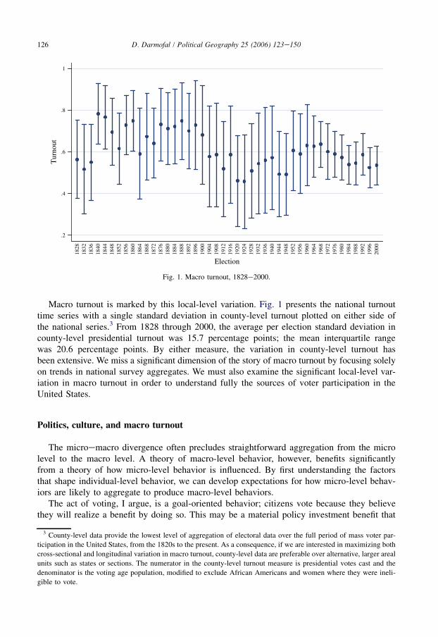
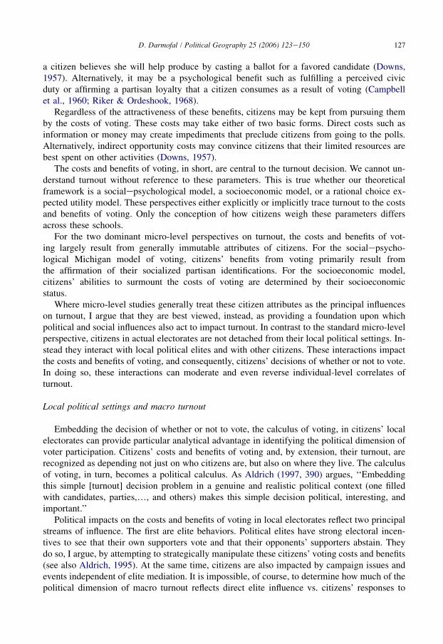
Macro turnout is marked by this local-level variation. Fig. 1 presents the national turnouttime series with a single standard deviation in county-level turnout plotted on either side ofthe national series.3 From 1828 through 2000, the average per election standard deviation incounty-level presidential turnout was 15.7 percentage points; the mean interquartile rangewas 20.6 percentage points. By either measure, the variation in county-level turnout hasbeen extensive. We miss a significant dimension of the story of macro turnout by focusing solelyon trends in national survey aggregates. We must also examine the significant local-level var-iation in macro turnout in order to understand fully the sources of voter participation in theUnited States.

Politics, culture, and macro turnout

The microemacro divergence often precludes straightforward aggregation from the microlevel to the macro level. A theory of macro-level behavior, however, benefits significantlyfrom a theory of how micro-level behavior is influenced. By first understanding the factorsthat shape individual-level behavior, we can develop expectations for how micro-level behav-iors are likely to aggregate to produce macro-level behaviors.

The act of voting, I argue, is a goal-oriented behavior; citizens vote because they believethey will realize a benefit by doing so. This may be a material policy investment benefit that

.2

.4

.6

.8

1

1828

1832

1836

1840

1844

1848

1852

1856

1860

1864

1868

1872

1876

1880

1884

1888

1892

1896

1900

1904

1908

1912

1916

1920

1924

1928

1932

1936

1940

1944

1948

1952

1956

1960

1964

1968

1972

1976

1980

1984

1988

1992

1996

2000

Tur

nout

Election

Fig. 1. Macro turnout, 1828e2000.

3 County-level data provide the lowest level of aggregation of electoral data over the full period of mass voter par-

ticipation in the United States, from the 1820s to the present. As a consequence, if we are interested in maximizing both

cross-sectional and longitudinal variation in macro turnout, county-level data are preferable over alternative, larger areal

units such as states or sections. The numerator in the county-level turnout measure is presidential votes cast and the

denominator is the voting age population, modified to exclude African Americans and women where they were ineli-

gible to vote.


a citizen believes she will help produce by casting a ballot for a favored candidate (Downs,1957). Alternatively, it may be a psychological benefit such as fulfilling a perceived civicduty or affirming a partisan loyalty that a citizen consumes as a result of voting (Campbellet al., 1960; Riker & Ordeshook, 1968).

Regardless of the attractiveness of these benefits, citizens may be kept from pursuing themby the costs of voting. These costs may take either of two basic forms. Direct costs such asinformation or money may create impediments that preclude citizens from going to the polls.Alternatively, indirect opportunity costs may convince citizens that their limited resources arebest spent on other activities (Downs, 1957).

The costs and benefits of voting, in short, are central to the turnout decision. We cannot un-derstand turnout without reference to these parameters. This is true whether our theoreticalframework is a socialepsychological model, a socioeconomic model, or a rational choice ex-pected utility model. These perspectives either explicitly or implicitly trace turnout to the costsand benefits of voting. Only the conception of how citizens weigh these parameters differsacross these schools.

For the two dominant micro-level perspectives on turnout, the costs and benefits of vot-ing largely result from generally immutable attributes of citizens. For the socialepsycho-logical Michigan model of voting, citizens’ benefits from voting primarily result fromthe affirmation of their socialized partisan identifications. For the socioeconomic model,citizens’ abilities to surmount the costs of voting are determined by their socioeconomicstatus.

Where micro-level studies generally treat these citizen attributes as the principal influenceson turnout, I argue that they are best viewed, instead, as providing a foundation upon whichpolitical and social influences also act to impact turnout. In contrast to the standard micro-levelperspective, citizens in actual electorates are not detached from their local political settings. In-stead they interact with local political elites and with other citizens. These interactions impactthe costs and benefits of voting, and consequently, citizens’ decisions of whether or not to vote.In doing so, these interactions can moderate and even reverse individual-level correlates ofturnout.

Local political settings and macro turnout

Embedding the decision of whether or not to vote, the calculus of voting, in citizens’ localelectorates can provide particular analytical advantage in identifying the political dimension ofvoter participation. Citizens’ costs and benefits of voting and, by extension, their turnout, arerecognized as depending not just on who citizens are, but also on where they live. The calculusof voting, in turn, becomes a political calculus. As Aldrich (1997, 390) argues, ‘‘Embeddingthis simple [turnout] decision problem in a genuine and realistic political context (one filledwith candidates, parties,., and others) makes this simple decision political, interesting, andimportant.’’

Political impacts on the costs and benefits of voting in local electorates reflect two principalstreams of influence. The first are elite behaviors. Political elites have strong electoral incen-tives to see that their own supporters vote and that their opponents’ supporters abstain. Theydo so, I argue, by attempting to strategically manipulate these citizens’ voting costs and benefits(see also Aldrich, 1995). At the same time, citizens are also impacted by campaign issues andevents independent of elite mediation. It is impossible, of course, to determine how much of thepolitical dimension of macro turnout reflects direct elite influence vs. citizens’ responses to


campaigns. We would expect, however, that in most electorates over the course of Americanpolitical development, this political dimension reflects both streams of influence.

Given elites’ incentives to be electorally active in local electorates, it is essential to examinehow elites seek to gain office by impacting citizens’ costs and benefits of voting. Elites seek tomobilize their supporters’ turnout by increasing their policy and psychological benefits of vot-ing and by reducing their direct and indirect costs of voting. They seek to demobilize opposi-tion turnout by reducing opposition supporters’ benefits of voting and by increasing their costsof voting.

Elites can increase their supporters’ policy differential benefits, as well as the consumptionbenefits that accompany these policy benefits (Fiorina, 1976), by drawing distinctions betweentheir own positions and their opponents’. And contrary to Downsian expectations about the me-dian voter, American parties’ policy positions do in fact diverge (Page, 1978). At the same time,this divergence is not universal across all issues. Elites have strategic incentives to mimic theiropponents’ positions on some issues or to take ambiguous positions (Page, 1976; Shepsle,1972). Such strategies can reduce the turnout of opposition supporters by reducing their policymotives for voting. Elites influence the cost side of the turnout ledger through campaign activ-ities and voting law enactments. Campaign speeches, debates, and paid advertising all aim toreduce supporters’ information costs. Get-out-the-vote efforts at the end of campaigns aim toreduce the monetary, time, and information costs of voting (Aldrich, 1995, 101).

Voting law enactments can be employed to increase opposition supporters’ costs of voting.There is an asymmetric political benefit from such voting law enactments. Because lower-classcitizens are likely to have the greatest difficulty clearing the hurdle to participation posed byrestrictive voting laws (Wolfinger and Rosenstone, 1980; but see Nagler, 1991), restrictive vot-ing laws provide a particularly attractive means for political elites representing upper-class in-terests to restrict the participation of lower-class opposition supporters.

The two streams of political influence shape the costs and benefits of voting via several po-litical dimensions of local electorates. Among these are the competitiveness of elections, thevigor of minor party campaigns, and the restrictiveness of voting laws. Each of these politicalfeatures of local electorates is likely to affect individuals’ turnout decisions and potentially pro-duce macro turnout variation across local electorates as a consequence.

As discussed earlier, translating implications from the micro to the macro level is not alwaysa straightforward process. Aggregation bias largely precludes predictions regarding point esti-mates of macro effects. Because macro-level coefficients are often correlated with their regres-sors, and because we have little a priori theory for modeling this correlation, we are generallyunable to predict how much a political feature of a local electorate will increase or decreasemacro turnout (Cho, 1998; King, 1997; Robinson, 1950).

Generally, however, our interest is not in point prediction but rather in directional prediction:is a political dimension of a local electorate likely to increase or reduce macro turnout? Evenhere, however, we will often encounter difficulties in formulating a priori expectations due tothe microemacro divergence. Political factors may shift the benefits or costs of voting (and thusthe probabilities of voting) in different directions for different citizens in a local electorate. Di-vergent micro-level effects preclude macro-level expectations.

Consider minor party candidacies. These candidacies may increase the policy or psycholog-ical benefits of voting for Independents and those disenchanted with the major party alternatives(and may reduce these citizens’ voting costs through mobilization campaigns). At the sametime, the issues raised by these candidacies may highlight the weaknesses in major party can-didacies, making partisan adherents less likely to vote. The result is no clear directional


prediction for macro-level turnout. A significant advantage of a macro-level approach, however,is that we are able to identify how factors with no clear directional predictions at the micro levelimpact the more consequential macro-level turnout. It is of considerable importance to identifyhow minor party candidacies and other factors with no clear micro-level predictions have im-pacted macro turnout over the course of American political development.

We can be more confident in our macro-level expectations when a political dimension islikely to shift citizens’ probabilities of voting in the same direction within a local electorate.Partisan competition carries these directionally consistent micro-level effects, producing a clearmacro-level expectation. Strategic political elites are more likely to mobilize citizens in closeelections (Cox & Munger, 1989). This is likely to increase the psychological benefits of votingwhile reducing the costs of voting (through get-out-the-vote efforts). Citizens are also likely tohave increased psychological motives for voting in competitive elections due to their increasedinterest in such contests. At the same time, citizens may have increased policy motives for vot-ing in such contests as they believe erroneously that their vote is likely to be decisive despitethe fact that the chances of casting a decisive ballot are infinitesimally small (Gelman, King, &Boscardin, 1998; Riker & Ordeshook, 1968).

It is unlikely that competitive elections will reduce voting benefits or increase voting costs,and thus reduce micro-level turnout. Partisan competition thus is expected to increase both mi-cro- and macro-level turnout. As a consequence, electorates with more competitive electionsshould have higher turnout than electorates with less competitive elections.

Political influences on macro turnout are also likely to promote a spatial structuring of turn-out rates that transcends local electorates. Similar levels of partisan competition, for example,are likely to exist in neighboring electorates, particularly as elites speak to shared interests thattranscend these electorates and imitate the mobilization activities of neighboring elites. Identi-fying the relationship between political dimensions, including partisan competition, and thespatial structuring of macro turnout is critical for understanding the political dimension of par-ticipation in American political development.

Elazar’s cultural thesis and macro turnout

Although the implications of local political dimensions for macro turnout and its spatialstructuring have been underexplored to date, an earlier research approach emphasizing the im-portance of local political culture for participation has received extensive consideration in theliterature (Elazar, 1984, 1994; Sharkansky, 1969). The principal cultural thesis is Elazar’s ac-count. Borrowing from Almond’s (1956, 396) definition, Elazar (1994, 214) defines politicalculture as ‘‘the particular pattern of orientations to political action in which each political sys-tem is embedded.’’ Elazar presents a tripartite thesis, in which he argues that locales are markedby moralistic, individualistic, or traditionalistic political cultures. These political cultures, Ela-zar argues, carry clear expectations for macro turnout rates.

The moralistic culture views politics as ‘‘the search for the good society . an effort to ex-ercise power for the betterment of the commonwealth’’ (Elazar, 1984, 117). Citizen participa-tion is valued and expected in this commonwealth conception of governance. For Elazar (1994,233), ‘‘this political culture considers it the duty of every citizen to participate in the politicalaffairs of his or her commonwealth.’’ As a consequence, electorates with moralistic politicalcultures should exhibit high turnout rates (Elazar, 1984, 1994).

At the opposite end of the political cultural spectrum is the traditionalistic culture. Where themoralistic culture values citizen participation, the traditionalistic culture discourages it. The


traditionalistic culture, Elazar argues, is built upon the notion of a natural social hierarchy. Inthe traditionalistic culture, ‘‘real political power [is confined] to a relatively small and self-per-petuating group drawn from an established elite who often inherit their right to govern throughfamily ties or social position’’ (Elazar, 1984, 119). Such a small sphere of power cannot be longmaintained if ordinary citizens are actively engaged in politics. As a result, Elazar (1994, 235)argues, in the traditionalistic culture, ‘‘those [ordinary citizens] who do not have a definite roleto play in politics are not expected to be even minimally active as citizens. In many cases, theyare not even expected to vote.’’ As a consequence, macro turnout should be low in electorateswith traditionalistic political cultures.

Between the two extremes of the political cultural continuum lies the individualistic cul-ture. Where the moralistic culture views society as a commonwealth and the traditionalisticculture views it as a hierarchy, the individualistic culture views it as a marketplace. Elazar(1994, 230) notes, ‘‘political participation in systems dominated by the individualistic politicalculture reflects the view that politics is just another means by which individuals may improvethemselves socially and economically.’’ Neither promoted by conceptions of the common-wealth nor discouraged by conceptions of hierarchy, macro turnout rates in the individualisticculture are expected to be between those in the moralistic and traditionalistic cultures (Shar-kansky, 1969).

Elazar’s political culture thesis has found empirical support in explaining aggregate turnoutrates. Coding states’ political cultures on a 9 point scale ranging from moralistic (1) to tradi-tionalistic (9), Sharkansky (1969, 71, 80) finds significant negative correlations between polit-ical culture and macro turnout at the state level, controlling for state-level characteristics suchas personal income and urbanism. Sharkansky’s (1969, 73) analysis, however, is static, focusingonly on the period of the early 1960s.

Elazar’s conception of political culture, in contrast, is not static. Instead, Elazar (1994, 216,217) argues that the geographic location of political cultures has depended upon ethnoculturalwaves of immigration, from the first European immigration during the Colonial era, to 19thcentury European and Canadian immigration, to 20th century Hispanic and Asian immigration.Elazar traces the moralistic political culture to Puritan, North Sea, and Jewish immigrationwaves and places this culture in the Northern tier of states from New England across the UpperPlains to the Pacific Northwest. Elazar traces the traditionalistic political culture to early Euro-pean agrarian immigration and places it in the South. Finally, Elazar traces the individualisticpolitical culture to several European immigration waves including English, Mediterranean, andIrish streams and places this culture in the Mid-Atlantic and Midwest states (Elazar, 1994,215e223, 230e237).

Elazar’s thesis thus provides clear expectations for the local spatial structuring of turnout inAmerican political development. Throughout American electoral history, local electorates inNew England should have been marked by high turnout rates due to their moralistic cultures.As Northern European immigration spread westward into the Upper Plains and Pacific North-west, local electorates in these locations should also have become marked by high turnout ratesdue to their moralistic cultures. Local electorates in the Middle Atlantic states, alternatively,should always evidence intermediate turnout rates due to their individualistic political cultures.Additionally, as westward expansion of the population and of the individualistic culture spreadacross the Midwest, local electorates in these states should also have become marked by interme-diate turnout rates as a result of their individualistic political cultures. Finally, local electorates inthe South should have been marked by low turnout rates from the beginning as the traditionalisticpolitical culture was present in the South from its beginning, even prior to the Jim Crow era.


The political geography of macro turnout in the United States, 1828e2000

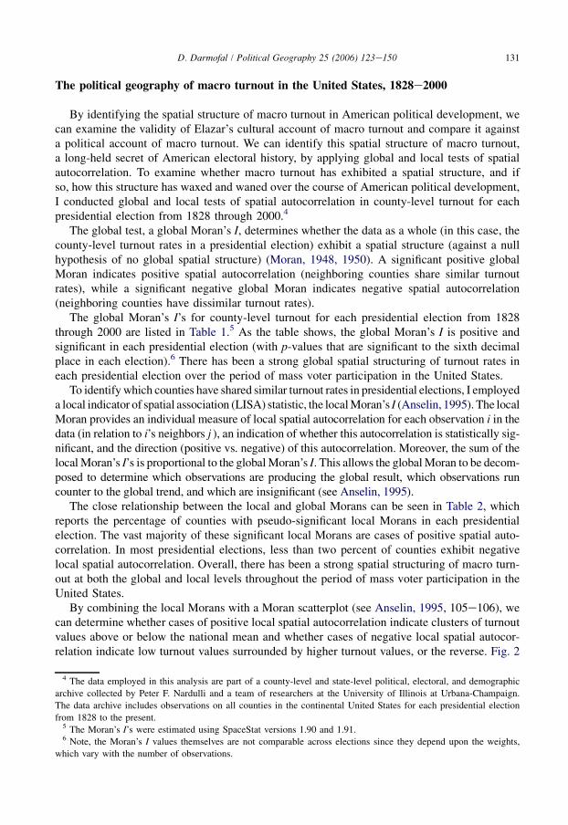
By identifying the spatial structure of macro turnout in American political development, wecan examine the validity of Elazar’s cultural account of macro turnout and compare it againsta political account of macro turnout. We can identify this spatial structure of macro turnout,a long-held secret of American electoral history, by applying global and local tests of spatialautocorrelation. To examine whether macro turnout has exhibited a spatial structure, and ifso, how this structure has waxed and waned over the course of American political development,I conducted global and local tests of spatial autocorrelation in county-level turnout for eachpresidential election from 1828 through 2000.4

The global test, a global Moran’s I, determines whether the data as a whole (in this case, thecounty-level turnout rates in a presidential election) exhibit a spatial structure (against a nullhypothesis of no global spatial structure) (Moran, 1948, 1950). A significant positive globalMoran indicates positive spatial autocorrelation (neighboring counties share similar turnoutrates), while a significant negative global Moran indicates negative spatial autocorrelation(neighboring counties have dissimilar turnout rates).

The global Moran’s I’s for county-level turnout for each presidential election from 1828through 2000 are listed in Table 1.5 As the table shows, the global Moran’s I is positive andsignificant in each presidential election (with p-values that are significant to the sixth decimalplace in each election).6 There has been a strong global spatial structuring of turnout rates ineach presidential election over the period of mass voter participation in the United States.

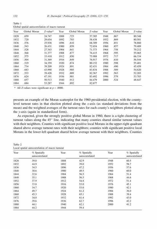
To identify which counties have shared similar turnout rates in presidential elections, I employeda local indicator of spatial association (LISA) statistic, the localMoran’s I (Anselin, 1995). The localMoran provides an individual measure of local spatial autocorrelation for each observation i in thedata (in relation to i’s neighbors j ), an indication of whether this autocorrelation is statistically sig-nificant, and the direction (positive vs. negative) of this autocorrelation. Moreover, the sum of thelocalMoran’s I’s is proportional to the globalMoran’s I. This allows the globalMoran to be decom-posed to determine which observations are producing the global result, which observations runcounter to the global trend, and which are insignificant (see Anselin, 1995).

The close relationship between the local and global Morans can be seen in Table 2, whichreports the percentage of counties with pseudo-significant local Morans in each presidentialelection. The vast majority of these significant local Morans are cases of positive spatial auto-correlation. In most presidential elections, less than two percent of counties exhibit negativelocal spatial autocorrelation. Overall, there has been a strong spatial structuring of macro turn-out at both the global and local levels throughout the period of mass voter participation in theUnited States.

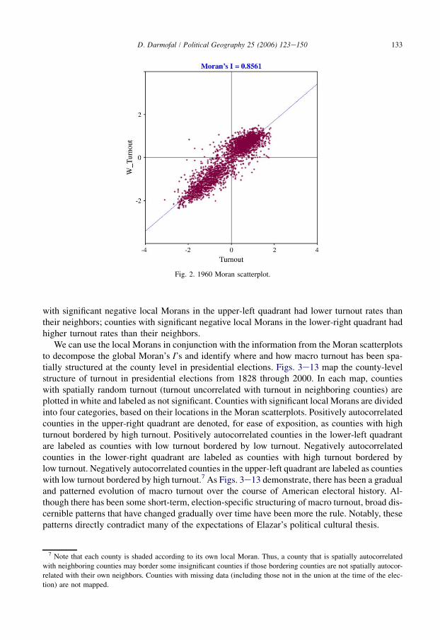
By combining the local Morans with a Moran scatterplot (see Anselin, 1995, 105e106), wecan determine whether cases of positive local spatial autocorrelation indicate clusters of turnoutvalues above or below the national mean and whether cases of negative local spatial autocor-relation indicate low turnout values surrounded by higher turnout values, or the reverse. Fig. 2

4 The data employed in this analysis are part of a county-level and state-level political, electoral, and demographic

archive collected by Peter F. Nardulli and a team of researchers at the University of Illinois at Urbana-Champaign.

The data archive includes observations on all counties in the continental United States for each presidential election

from 1828 to the present.5 The Moran’s I’s were estimated using SpaceStat versions 1.90 and 1.91.6 Note, the Moran’s I values themselves are not comparable across elections since they depend upon the weights,

which vary with the number of observations.


presents an example of the Moran scatterplot for the 1960 presidential election, with the county-level turnout rates in that election plotted along the x-axis (as standard deviations from themean) and the weighted averages of the turnout rates for each county’s neighbors plotted alongthe y-axis (again in standardized form).

As expected, given the strongly positive global Moran in 1960, there is a tight clustering ofturnout values along the 45 � line, indicating that many counties shared similar turnout valueswith their neighbors. Counties with significant positive local Morans in the upper-right quadrantshared above average turnout rates with their neighbors; counties with significant positive localMorans in the lower-left quadrant shared below average turnout with their neighbors. Counties

Table 1

Global spatial autocorrelation of macro turnout

Year Global Moran Z-value* Year Global Moran Z-value Year Global Moran Z-value

1828 .659 24.747 1888 .723 57.305 1948 .867 80.348

1832 .720 29.654 1892 .703 58.438 1952 .869 80.501

1836 .576 25.938 1896 .810 68.309 1956 .851 78.860

1840 .543 26.431 1900 .859 72.654 1960 .857 79.409

1844 .528 27.343 1904 .841 71.373 1964 .758 70.212

1848 .568 31.377 1908 .877 76.415 1968 .595 55.065

1852 .575 33.410 1912 .850 75.988 1972 .717 66.334

1856 .504 31.369 1916 .849 76.917 1976 .610 56.544

1860 .519 34.359 1920 .874 80.152 1980 .598 55.401

1864 .734 39.209 1924 .891 82.431 1984 .490 45.459

1868 .683 43.990 1928 .905 83.834 1988 .589 54.620

1872 .533 39.428 1932 .889 82.367 1992 .563 52.203

1876 .624 47.191 1936 .901 83.492 1996 .579 53.703

1880 .657 50.513 1940 .912 84.479 2000 .524 48.647

1884 .684 53.287 1944 .892 82.677

* All Z-values were significant at p< .0000.

Table 2

Local spatial autocorrelation of macro turnout

Year % Spatially

autocorrelated

Year % Spatially

autocorrelated

Year % Spatially

autocorrelated

1828 39.0 1888 42.9 1948 60.5

1832 44.9 1892 39.0 1952 58.7

1836 34.5 1896 47.2 1956 57.6

1840 30.6 1900 49.5 1960 60.0

1844 32.6 1904 56.5 1964 51.4

1848 35.1 1908 56.5 1968 44.6

1852 37.9 1912 54.8 1972 51.4

1856 33.8 1916 53.0 1976 45.1

1860 34.7 1920 53.0 1980 42.1

1864 49.7 1924 61.2 1984 36.0

1868 45.3 1928 65.1 1988 39.4

1872 34.0 1932 61.4 1992 43.0

1876 39.6 1936 62.7 1996 42.2

1880 44.1 1940 62.1 2000 41.2

1884 44.2 1944 59.4


with significant negative local Morans in the upper-left quadrant had lower turnout rates thantheir neighbors; counties with significant negative local Morans in the lower-right quadrant hadhigher turnout rates than their neighbors.

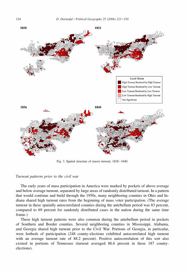
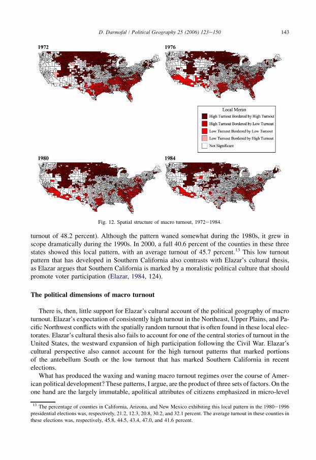
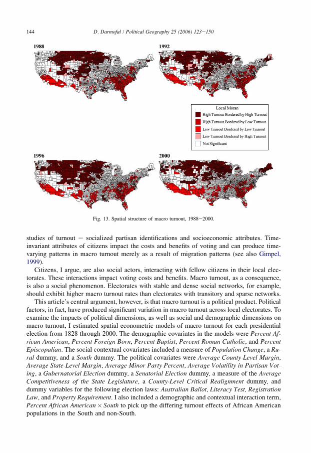
We can use the local Morans in conjunction with the information from the Moran scatterplotsto decompose the global Moran’s I’s and identify where and how macro turnout has been spa-tially structured at the county level in presidential elections. Figs. 3e13 map the county-levelstructure of turnout in presidential elections from 1828 through 2000. In each map, countieswith spatially random turnout (turnout uncorrelated with turnout in neighboring counties) areplotted in white and labeled as not significant. Counties with significant local Morans are dividedinto four categories, based on their locations in the Moran scatterplots. Positively autocorrelatedcounties in the upper-right quadrant are denoted, for ease of exposition, as counties with highturnout bordered by high turnout. Positively autocorrelated counties in the lower-left quadrantare labeled as counties with low turnout bordered by low turnout. Negatively autocorrelatedcounties in the lower-right quadrant are labeled as counties with high turnout bordered bylow turnout. Negatively autocorrelated counties in the upper-left quadrant are labeled as countieswith low turnout bordered by high turnout.7 As Figs. 3e13 demonstrate, there has been a gradualand patterned evolution of macro turnout over the course of American electoral history. Al-though there has been some short-term, election-specific structuring of macro turnout, broad dis-cernible patterns that have changed gradually over time have been more the rule. Notably, thesepatterns directly contradict many of the expectations of Elazar’s political cultural thesis.

Fig. 2. 1960 Moran scatterplot.

7 Note that each county is shaded according to its own local Moran. Thus, a county that is spatially autocorrelated

with neighboring counties may border some insignificant counties if those bordering counties are not spatially autocor-

related with their own neighbors. Counties with missing data (including those not in the union at the time of the elec-

tion) are not mapped.


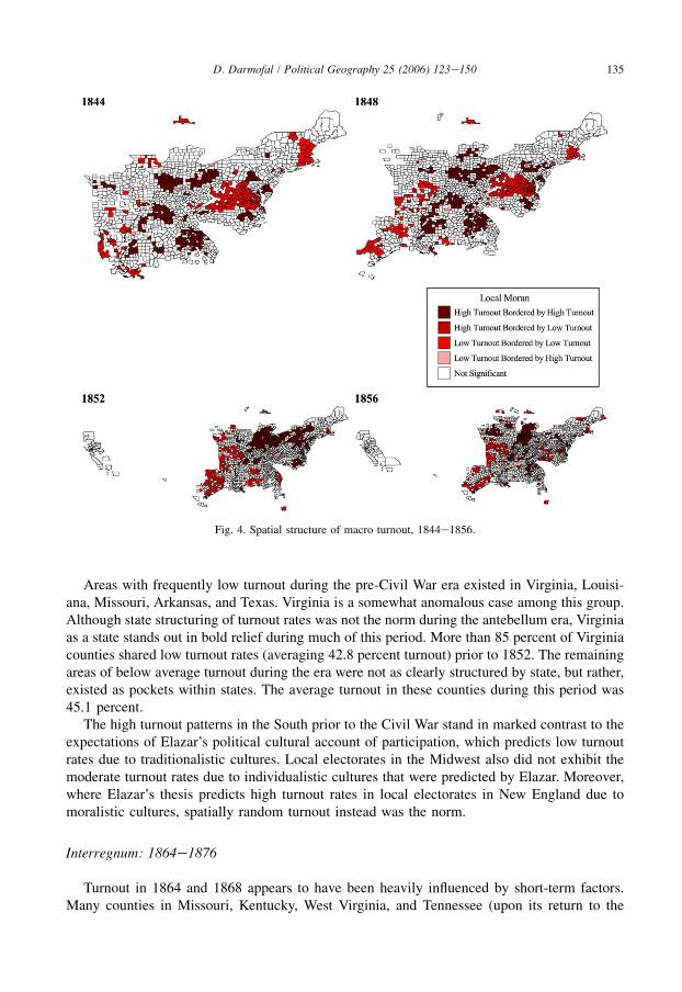
Turnout patterns prior to the civil war

The early years of mass participation in America were marked by pockets of above averageand below average turnout, separated by large areas of randomly distributed turnout. In a patternthat would continue and build through the 1950s, many neighboring counties in Ohio and In-diana shared high turnout rates from the beginning of mass voter participation. (The averageturnout in these spatially autocorrelated counties during the antebellum period was 83 percent,compared to 69 percent for randomly distributed cases in the nation during the same timeframe.)

These high turnout patterns were also common during the antebellum period in pocketsof Southern and Border counties. Several neighboring counties in Mississippi, Alabama,and Georgia shared high turnout prior to the Civil War. Portions of Georgia, in particular,were hotbeds of participation (248 county-elections exhibited autocorrelated high turnoutwith an average turnout rate of 88.2 percent). Positive autocorrelation of this sort alsoexisted in portions of Tennessee (turnout averaged 86.6 percent in these 187 county-elections).

Fig. 3. Spatial structure of macro turnout, 1828e1840.


Areas with frequently low turnout during the pre-Civil War era existed in Virginia, Louisi-ana, Missouri, Arkansas, and Texas. Virginia is a somewhat anomalous case among this group.Although state structuring of turnout rates was not the norm during the antebellum era, Virginiaas a state stands out in bold relief during much of this period. More than 85 percent of Virginiacounties shared low turnout rates (averaging 42.8 percent turnout) prior to 1852. The remainingareas of below average turnout during the era were not as clearly structured by state, but rather,existed as pockets within states. The average turnout in these counties during this period was45.1 percent.

The high turnout patterns in the South prior to the Civil War stand in marked contrast to theexpectations of Elazar’s political cultural account of participation, which predicts low turnoutrates due to traditionalistic cultures. Local electorates in the Midwest also did not exhibit themoderate turnout rates due to individualistic cultures that were predicted by Elazar. Moreover,where Elazar’s thesis predicts high turnout rates in local electorates in New England due tomoralistic cultures, spatially random turnout instead was the norm.

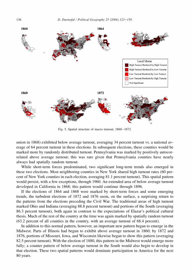
Interregnum: 1864e1876

Turnout in 1864 and 1868 appears to have been heavily influenced by short-term factors.Many counties in Missouri, Kentucky, West Virginia, and Tennessee (upon its return to the



union in 1868) exhibited below average turnout, averaging 34 percent turnout vs. a national av-erage of 64 percent turnout in these elections. In subsequent elections, these counties would bemarked more by randomly distributed turnout. Pennsylvania was marked by positively autocor-related above average turnout; this was rare given that Pennsylvania counties have nearlyalways had spatially random turnout.

While short-term forces predominated, two significant long-term trends also emerged inthese two elections. Most neighboring counties in New York shared high turnout rates (60 per-cent of New York counties in each election, averaging 81.1 percent turnout). This spatial patternwould persist, with a few exceptions, through 1960. An extended area of below average turnoutdeveloped in California in 1868; this pattern would continue through 1896.

If the elections of 1864 and 1868 were marked by short-term forces and some emergingtrends, the turbulent elections of 1872 and 1876 seem, on the surface, a surprising return tothe patterns from the elections preceding the Civil War. The traditional areas of high turnoutmarked Ohio and Indiana (averaging 88.8 percent turnout) and portions of the South (averaging86.3 percent turnout), both again in contrast to the expectations of Elazar’s political culturalthesis. Much of the rest of the country at the time was again marked by spatially random turnout(63.2 percent of all counties in the country, with an average turnout of 68.4 percent).

In addition to this normal pattern, however, an important new pattern began to emerge in theMidwest. Parts of Illinois had begun to exhibit above average turnout in 1860; by 1872 and1876, portions of Missouri, Iowa, and Wisconsin likewise began to show this pattern (averaging82.5 percent turnout). With the election of 1880, this pattern in the Midwest would emerge morefully; a counter pattern of below average turnout in the South would also begin to develop inthat election. These two spatial patterns would dominate participation in America for the next80 years.



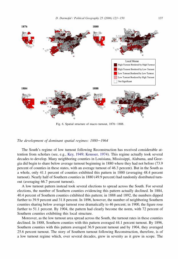
The development of dominant spatial regimes: 1880e1964

The South’s regime of low turnout following Reconstruction has received considerable at-tention from scholars (see, e.g., Key, 1949; Kousser, 1974). This regime actually took severaldecades to develop. Many neighboring counties in Louisiana, Mississippi, Alabama, and Geor-gia did begin to share below average turnout beginning in 1880 where they had not before (73.9percent of counties in these states, with an average turnout of 46.3 percent). But in the South asa whole, only 41.1 percent of counties exhibited this pattern in 1880 (averaging 48.4 percentturnout). Nearly half of Southern counties in 1880 (49.9 percent) had randomly distributed turn-out (averaging 66.7 percent turnout).

A low turnout pattern instead took several elections to spread across the South. For severalelections, the number of Southern counties evidencing this pattern actually declined. In 1884,40.4 percent of Southern counties exhibited this pattern; in 1888 and 1892, the numbers dippedfurther to 39.9 percent and 31.8 percent. In 1896, however, the number of neighboring Southerncounties sharing below average turnout rose dramatically to 46 percent; in 1900, the figure rosefurther to 51.1 percent. By 1904, the pattern had clearly become the norm, with 72 percent ofSouthern counties exhibiting this local structure.

Moreover, as the low turnout area spread across the South, the turnout rates in these countiesdeclined. In 1888, Southern counties with this pattern averaged 44.1 percent turnout. By 1896,Southern counties with this pattern averaged 36.9 percent turnout and by 1904, they averaged25.6 percent turnout. The story of Southern turnout following Reconstruction, therefore, is ofa low turnout regime which, over several decades, grew in severity as it grew in scope. The



pattern of below average turnout throughout the South would persist through 1964, when 67.6percent of Southern counties exhibited this pattern.

The several decades of declining turnout in the South following Reconstruction again standin contrast to the expectations of Elazar’s thesis. The traditionalistic culture, Elazar had argued,had long marked the South and should have produced consistently low turnout rates. The pat-tern of low turnout that developed following the end of Reconstruction suggests the influence,instead, of political features of local electorates, such as a decline in partisan competition andthe enactment of restrictive voting laws (Darmofal, 2003). The patterns are consistent not witha cultural account, which in this particular instance predicts a time-invariant pattern, but in-stead, with a political account that recognizes the impact of partisan competition and eliteactivities.

Although the low turnout regime in the South has received a great deal of attention frompolitical scientists and historians, the development of a high turnout regime in Midwest andPlains counties during the same period has received far less attention. Indeed, one of the greatuntold stories of voter turnout in American history has been this westward expansion of partic-ipation. At its high point in the early 1940s, this spatial pattern would encompass nearly a thirdof the counties in the continental United States.

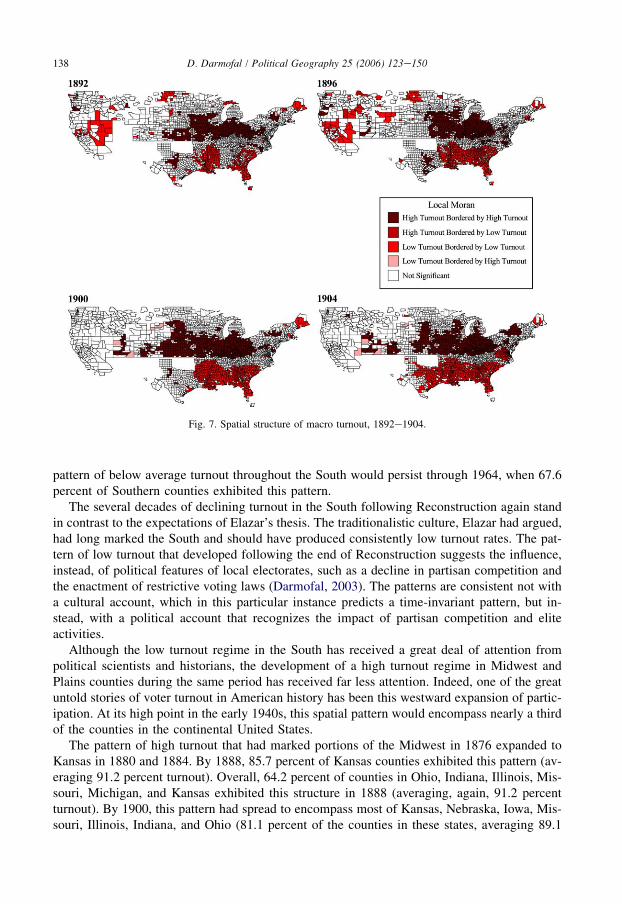
The pattern of high turnout that had marked portions of the Midwest in 1876 expanded toKansas in 1880 and 1884. By 1888, 85.7 percent of Kansas counties exhibited this pattern (av-eraging 91.2 percent turnout). Overall, 64.2 percent of counties in Ohio, Indiana, Illinois, Mis-souri, Michigan, and Kansas exhibited this structure in 1888 (averaging, again, 91.2 percentturnout). By 1900, this pattern had spread to encompass most of Kansas, Nebraska, Iowa, Mis-souri, Illinois, Indiana, and Ohio (81.1 percent of the counties in these states, averaging 89.1



percent turnout). With minor short-term fluctuations, this spatial pattern of above average turn-out persisted through the 1916 election.

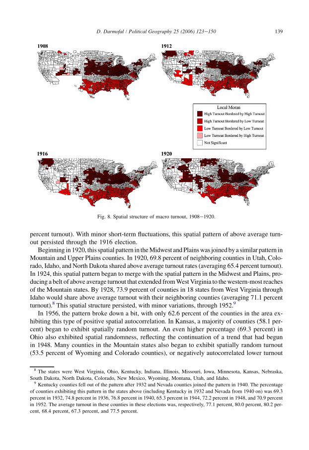
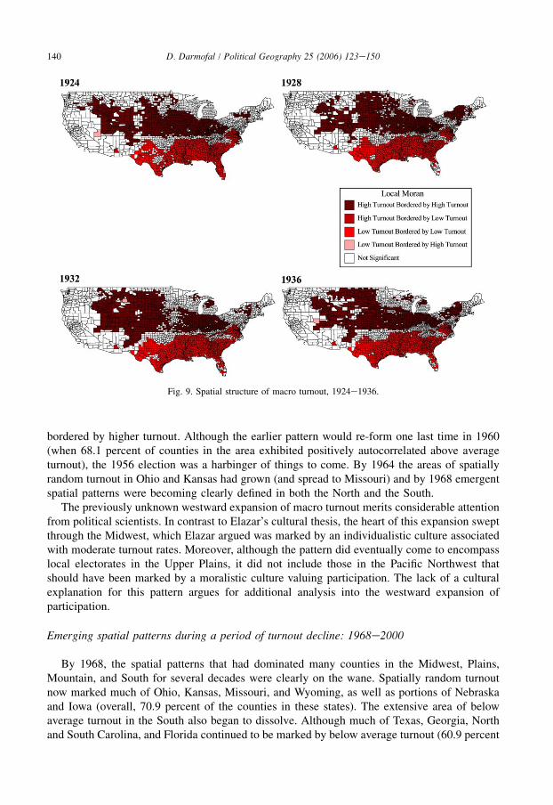
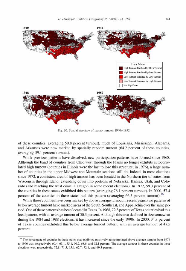
Beginning in 1920, this spatial pattern in theMidwest andPlainswas joinedbya similar pattern inMountain and Upper Plains counties. In 1920, 69.8 percent of neighboring counties in Utah, Colo-rado, Idaho, and North Dakota shared above average turnout rates (averaging 65.4 percent turnout).In 1924, this spatial pattern began to merge with the spatial pattern in the Midwest and Plains, pro-ducing a belt of above average turnout that extended fromWestVirginia to thewestern-most reachesof the Mountain states. By 1928, 73.9 percent of counties in 18 states from West Virginia throughIdaho would share above average turnout with their neighboring counties (averaging 71.1 percentturnout).8 This spatial structure persisted, with minor variations, through 1952.9

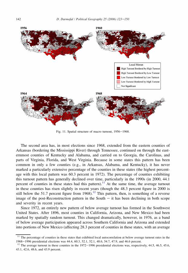
In 1956, the pattern broke down a bit, with only 62.6 percent of the counties in the area ex-hibiting this type of positive spatial autocorrelation. In Kansas, a majority of counties (58.1 per-cent) began to exhibit spatially random turnout. An even higher percentage (69.3 percent) inOhio also exhibited spatial randomness, reflecting the continuation of a trend that had begunin 1948. Many counties in the Mountain states also began to exhibit spatially random turnout(53.5 percent of Wyoming and Colorado counties), or negatively autocorrelated lower turnout


8 The states were West Virginia, Ohio, Kentucky, Indiana, Illinois, Missouri, Iowa, Minnesota, Kansas, Nebraska,

South Dakota, North Dakota, Colorado, New Mexico, Wyoming, Montana, Utah, and Idaho.9 Kentucky counties fell out of the pattern after 1932 and Nevada counties joined the pattern in 1940. The percentage

of counties exhibiting this pattern in the states above (including Kentucky in 1932 and Nevada from 1940 on) was 69.3

percent in 1932, 74.8 percent in 1936, 76.8 percent in 1940, 65.3 percent in 1944, 72.2 percent in 1948, and 70.9 percent

in 1952. The average turnout in these counties in these elections was, respectively, 77.1 percent, 80.0 percent, 80.2 per-

cent, 68.4 percent, 67.3 percent, and 77.5 percent.


bordered by higher turnout. Although the earlier pattern would re-form one last time in 1960(when 68.1 percent of counties in the area exhibited positively autocorrelated above averageturnout), the 1956 election was a harbinger of things to come. By 1964 the areas of spatiallyrandom turnout in Ohio and Kansas had grown (and spread to Missouri) and by 1968 emergentspatial patterns were becoming clearly defined in both the North and the South.

The previously unknown westward expansion of macro turnout merits considerable attentionfrom political scientists. In contrast to Elazar’s cultural thesis, the heart of this expansion sweptthrough the Midwest, which Elazar argued was marked by an individualistic culture associatedwith moderate turnout rates. Moreover, although the pattern did eventually come to encompasslocal electorates in the Upper Plains, it did not include those in the Pacific Northwest thatshould have been marked by a moralistic culture valuing participation. The lack of a culturalexplanation for this pattern argues for additional analysis into the westward expansion ofparticipation.

Emerging spatial patterns during a period of turnout decline: 1968e2000

By 1968, the spatial patterns that had dominated many counties in the Midwest, Plains,Mountain, and South for several decades were clearly on the wane. Spatially random turnoutnow marked much of Ohio, Kansas, Missouri, and Wyoming, as well as portions of Nebraskaand Iowa (overall, 70.9 percent of the counties in these states). The extensive area of belowaverage turnout in the South also began to dissolve. Although much of Texas, Georgia, Northand South Carolina, and Florida continued to be marked by below average turnout (60.9 percent



of these counties, averaging 50.8 percent turnout), much of Louisiana, Mississippi, Alabama,and Arkansas were now marked by spatially random turnout (64.2 percent of these counties,averaging 59.1 percent turnout).

While previous patterns have dissolved, new participation patterns have formed since 1968.Although the band of counties from Ohio west through the Plains no longer exhibits autocorre-lated high turnout (counties in Illinois were the last to lose this structure, in 1976), a large num-ber of counties in the upper Midwest and Mountain sections still do. Indeed, in most electionssince 1972, a consistent area of high turnout has been located in the Northern tier of states fromWisconsin through Idaho, extending down into portions of Nebraska, Kansas, Utah, and Colo-rado (and reaching the west coast in Oregon in some recent elections). In 1972, 59.3 percent ofthe counties in these states exhibited this pattern (averaging 76.1 percent turnout). In 2000, 57.4percent of the counties in these states had this pattern (averaging 66.3 percent turnout).10

While these counties have beenmarked by above average turnout in recent years, two patterns ofbelow average turnout havemarked areas of the South, Southeast, andAppalachia over the same pe-riod.One of these patterns has been located in Texas. In 1968, 72.8 percent ofTexas counties had thislocal pattern, with an average turnout of 50.3 percent. Although this area declined in size somewhatduring the 1984 and 1988 elections, it has increased since the early 1990s. In 2000, 34.8 percentof Texas counties exhibited this below average turnout pattern, with an average turnout of 47.5percent.


10 The percentage of counties in these states that exhibited positively autocorrelated above average turnout from 1976

to 1996 was, respectively, 60.4, 65.1, 55.1, 60.7, 68.6, and 62.1 percent. The average turnout in these counties in these

elections was, respectively, 72.8, 71.5, 65.6, 67.7, 72.1, and 69.3 percent.


The second area has, in most elections since 1968, extended from the eastern counties ofArkansas (bordering the Mississippi River) through Tennessee, continued on through the east-ernmost counties of Kentucky and Alabama, and carried on to Georgia, the Carolinas, andparts of Virginia, Florida, and West Virginia. Because in some states this pattern has beencommon in only a few counties (e.g., in Arkansas, Alabama, and Kentucky), it has nevermarked a particularly extensive percentage of the counties in these states (the highest percent-age with this local pattern was 60.3 percent in 1972). The percentage of counties exhibitingthis turnout pattern has generally declined over time, particularly in the 1990s (in 2000, 44.1percent of counties in these states had this pattern).11 At the same time, the average turnoutin these counties has risen slightly in recent years (though the 48.3 percent figure in 2000 isstill below the 51.7 percent figure from 1968).12 This pattern, then, is something of a reverseimage of the post-Reconstruction pattern in the South e it has been declining in both scopeand severity in recent years.

Since 1972, an entirely new pattern of below average turnout has formed in the SouthwestUnited States. After 1896, most counties in California, Arizona, and New Mexico had beenmarked by spatially random turnout. This changed dramatically, however, in 1976, as a bandof below average participation appeared across Southern California and Arizona and extendedinto portions of New Mexico (affecting 28.3 percent of counties in these states, with an average


11 The percentage of counties in these states that exhibited local autocorrelation at below average turnout rates in the

1968e1996 presidential elections was 44.4, 60.3, 52.1, 52.1, 48.6, 54.7, 47.9, and 46.6 percent.12 The average turnout in these counties in the 1972e1996 presidential elections was, respectively, 44.5, 46.5, 45.6,

43.1, 42.6, 48.6, and 43.9 percent.


turnout of 48.2 percent). Although the pattern waned somewhat during the 1980s, it grew inscope dramatically during the 1990s. In 2000, a full 40.6 percent of the counties in these threestates showed this local pattern, with an average turnout of 45.7 percent.13 This low turnoutpattern that has developed in Southern California also contrasts with Elazar’s cultural thesis,as Elazar argues that Southern California is marked by a moralistic political culture that shouldpromote voter participation (Elazar, 1984, 124).

The political dimensions of macro turnout

There is, then, little support for Elazar’s cultural account of the political geography of macroturnout. Elazar’s expectation of consistently high turnout in the Northeast, Upper Plains, and Pa-cific Northwest conflicts with the spatially random turnout that is often found in these local elec-torates. Elazar’s cultural thesis also fails to account for one of the central stories of turnout in theUnited States, the westward expansion of high participation following the Civil War. Elazar’scultural perspective also cannot account for the high turnout patterns that marked portionsof the antebellum South or the low turnout that has marked Southern California in recentelections.

What has produced the waxing and waning macro turnout regimes over the course of Amer-ican political development? These patterns, I argue, are the product of three sets of factors. On theone hand are the largely immutable, apolitical attributes of citizens emphasized in micro-level


13 The percentage of counties in California, Arizona, and New Mexico exhibiting this local pattern in the 1980e1996

presidential elections was, respectively, 21.2, 12.3, 20.8, 30.2, and 32.1 percent. The average turnout in these counties in

these elections was, respectively, 45.8, 44.5, 43.4, 47.0, and 41.6 percent.


studies of turnout e socialized partisan identifications and socioeconomic attributes. Time-invariant attributes of citizens impact the costs and benefits of voting and can produce time-varying patterns in macro turnout merely as a result of migration patterns (see also Gimpel,1999).

Citizens, I argue, are also social actors, interacting with fellow citizens in their local elec-torates. These interactions impact voting costs and benefits. Macro turnout, as a consequence,is also a social phenomenon. Electorates with stable and dense social networks, for example,should exhibit higher macro turnout rates than electorates with transitory and sparse networks.

This article’s central argument, however, is that macro turnout is a political product. Politicalfactors, in fact, have produced significant variation in macro turnout across local electorates. Toexamine the impacts of political dimensions, as well as social and demographic dimensions onmacro turnout, I estimated spatial econometric models of macro turnout for each presidentialelection from 1828 through 2000. The demographic covariates in the models were Percent Af-rican American, Percent Foreign Born, Percent Baptist, Percent Roman Catholic, and PercentEpiscopalian. The social contextual covariates included a measure of Population Change, a Ru-ral dummy, and a South dummy. The political covariates were Average County-Level Margin,Average State-Level Margin, Average Minor Party Percent, Average Volatility in Partisan Vot-ing, a Gubernatorial Election dummy, a Senatorial Election dummy, a measure of the AverageCompetitiveness of the State Legislature, a County-Level Critical Realignment dummy, anddummy variables for the following election laws: Australian Ballot, Literacy Test, RegistrationLaw, and Property Requirement. I also included a demographic and contextual interaction term,Percent African American� South to pick up the differing turnout effects of African Americanpopulations in the South and non-South.



In each election other than the 1828 and 1836 elections, JarqueeBera test rejected the null ofnormally distributed errors ( p< .01, one-tailed test). Non-normality in errors compromises theLagrange Multiplier and Robust Lagrange Multiplier tests for spatial lag and spatial error de-pendence, as these tests assume normally distributed errors (Anselin & Bera, 1998). The Kele-jian and Robinson (1992) test for spatial error dependence, which does not require normality inerrors, indicated significant spatial error dependence from unmeasured covariates in each pres-idential election. There was, therefore, clear evidence of spatial error dependence and no clearevidence of contagion, or spatial lag dependence. As a result, I estimated spatial error modelsfor each election. The estimates for each election, not reported here due to space limitations, arereported in Darmofal (2003). Overall, political covariates account, on average, for an 11.6 pointturnout difference per election between positively autocorrelated above average and below av-erage turnout electorates.14

Earlier I discussed a particular political dimension e partisan competition e that presentsa clear macro-level directional turnout expectation due to its consistent micro-level directionalturnout effects. High and low turnout electorates have, in fact, been marked by significantlydifferent rates of competition for much of American political development. Throughout mostof American electoral history, local electorates with spatially autocorrelated above averageturnout have had significantly more competitive presidential elections than have local elector-ates with spatially autocorrelated below average turnout.15 A one-way analysis of varianceshows that positively autocorrelated above average turnout counties had significantly smallerpresidential election margins, on average, than positively autocorrelated below average turnoutcounties in 40 out of 44 presidential elections from 1828 through 2000 ( p< .001, one-tailedBonferroni test).16

Partisan competition also had a significant substantive impact on turnout differences be-tween high and low turnout regimes for much of American political development. Even aftercontrolling for a set of demographic, social, and other political influences on macro turnout,partisan competition still retained a significant role in producing turnout differences between

14 Political factors also influence anomalies in the political geography of macro turnout. Consider, for example, New

York, with its large band of spatially autocorrelated above average turnout in 1904, its smaller bands of such turnout in

1892 and 1900, and its near absence of such a structure in 1896. Because New York was long a critical swing state, New

Yorkers were common figures on national tickets in the late 19th and early 20th centuries. The 1896 election was the

lone election with no New Yorker on either major party ticket during this period. In 1892, in contrast, the Democratic

Presidential and Republican Vice-Presidential candidates were from New York. In 1900, the Republican Vice-Presiden-

tial candidate was from New York. And in 1904, both the Republican and Democratic Presidential candidates (Theodore

Roosevelt and Alton B. Parker, respectively) hailed from New York (CQ Press, 1997). As we would expect, the spatial

structuring of above average turnout in New York was strongest in the 1904 election, and weakest in the 1896 election,

with 1892 and 1900 as intermediate cases. Similarly, political factors also influenced the anomalous state structuring of

below average turnout in Virginia prior to 1852. For example, Virginia had significantly less competitive presidential

elections on average than other states during this period, p< .001, one-tailed two-sample t test.15 I measure local partisan competition in presidential elections using a five-election moving average that includes the

margin in the four preceding presidential elections and the margin in the current presidential election. Such a moving

average measure has the advantage of tapping both retrospective and prospective competitiveness. By incorporating past

competitiveness, the measure also incorporates the long-term competitiveness of elections in an electorate and reduces

the problem of potential endogeneity inherent in a single-election measure in which turnout may impact competitive-

ness rather than vice versa.16 The lone exceptions were the elections of 1840, 1844, 1848, and 1968, each of which had no significant difference in

average presidential margin between the two sets of counties. Positively autocorrelated high turnout electorates also had

significantly smaller average margins than spatially random electorates in 27 out of 44 presidential elections (one-way

ANOVA, p< .001, one-tailed Bonferroni test).


spatially autocorrelated above average and below average turnout electorates. From 1852through 1896, differences in average presidential margins accounted for one to three percentagepoints of the turnout difference between the two sets of counties.17 From 1900 through 1948,this impact grew larger, ranging from four to six percentage points.

Partisan competition has had a much reduced impact on turnout differences between highand low turnout counties, however, since 1960. Indeed, the United States appears to have en-tered into a distinct political era since the 1960s. Although political factors continue to affectmacro turnout, the nature of this impact has changed. For example, where state-level presiden-tial election competitiveness and state legislative competitiveness once produced significantturnout differences between high and low turnout electorates, this is no longer the case (Dar-mofal, 2003). These differing effects over time highlight the dynamic nature of the Americanpolity and the utility of longitudinal data for identifying the time-varying sources of macroturnout.18

Minor-party candidacies and macro turnout

Earlier I discussed the lack of a clear macro-level prediction for the turnout impact of minorparty candidacies due to potentially differing micro-level effects among citizens in the samelocal electorate. A critical advantage of the macro-level perspective, I argued, was the abilityto examine the macro impacts of such factors where we have conflicting micro-level expecta-tions. It is instructive, therefore, to examine the effects of minor party candidacies on macroturnout. These impacts have been time-variant, changing over the course of political party de-velopment in the United States.

Minor party support has had an oscillating, but often consequential relationship with macroturnout. During the Second American Party System, from 1828 through 1856, minor party sup-port in local electorates exerted no impact on macro turnout differences between spatially

17 The lone exception during this period was the 1860 election, in which presidential margins had no effect on turnout

differences between the two regimes.18 Immigration, women’s suffrage, and the rural vs. urban cleavage have all played critical roles in American political

development. The first two impacted the political geography of macro turnout while the third did not. Electorates with

spatially autocorrelated above average turnout have generally had larger foreign-born populations than have electorates

with spatially autocorrelated below average turnout. From 1880 through 1920, these larger immigrant populations were

associated with one to three points lower turnout in the former electorates than in the latter electorates. The much larger

immigrant populations in major Midwest urban centers such as Chicago, St. Louis, and Kansas City partially explain

why these locations were often excluded from the westward expansion of macro turnout following the Civil War. In

Cook County, IL, for example, 34 percent of the population was foreign born in 1904, vs. a national average of 9.3

percent. From 1924 through 1956, however, larger immigrant populations were associated with one to two points higher

turnout in spatially autocorrelated above average turnout electorates than in spatially autocorrelated below average turn-

out electorates. With aggregate data alone, we cannot tell whether these turnout differences were due to the (non)-voting

of immigrants or the (non)-voting of non-immigrants. It is suggestive, however, that the emergence of positive macro

turnout effects with larger immigrant populations coincides with the emergence of the modern, urban, ethnic Democratic

party in the 1920s. In contrast to immigrant populations, there has not been sufficient variation in male vs. female

populations across local electorates to produce significant variation in macro turnout across electorates. Several predom-

inantly western states, however, recognized women’s right to vote beginning in the late 19th century. These early adop-

tions were related to the political geography of macro turnout. Electorates with spatially autocorrelated above average

turnout were significantly more likely to have early adoptions of women’s suffrage than were electorates with spatially

autocorrelated below average turnout (one-way ANOVA, p< .01, one-tailed Bonferroni test). After controlling for po-

litical, social, and demographic factors, the rural vs. urban cleavage has had little independent effect on macro turnout.

In most elections, the Rural dummy variable has had no effect on the political geography of macro turnout.


autocorrelated above average and below average turnout electorates.19 As a minor party, theRepublicans, emerged to offer a vessel for opposition to slavery at the beginning of the ThirdAmerican Party System (1860e1896), support for minor parties briefly produced higher turnoutrates in spatially autocorrelated high turnout electorates than in spatially autocorrelated lowturnout electorates.20 As the Republican and Democratic parties increased their salience andtheir mobilization capacities during the latter quarter of the 19th century, minor parties ceasedto boost macro turnout.

The Republican and Democratic parties were weakened both in their salience with votersand as mobilizing organizations as a result of Progressive reforms at the beginning of the FourthAmerican Party System (1896e1932). However, this weakening of the major parties did notresult in minor party alternatives boosting macro turnout rates. Despite the considerable elec-toral support for minor parties such as the Progressives and Socialists during this period, minorparty support did not translate into higher macro turnout rates. Instead, minor parties had noeffect in producing turnout differences between spatially autocorrelated above average and be-low average turnout electorates until the 1920s. And at that point, where minor parties ranstrongest, macro turnout was generally lowest.

The emergence of the Democratic Party as the majority party in the United States at the be-ginning of the Fifth American Party System (1932epresent) brought with it a partial rehabil-itation in major party salience and organizational capacities. But despite the increasedprominence and attractiveness of the major parties (particularly the Democrats), minor partycandidacies still emerged. The States’ Rights (Dixiecrats) and Progressive Party candidaciesof 1948 briefly boosted macro turnout rates. Subsequently, minor party candidacies had littleconsequential impact on macro turnout for several decades.

Recent elections, however, have witnessed the largest macro turnout impacts of minor partycandidacies in American electoral history. From 1992 through 2000, minor party support pro-duced a five to six point turnout difference between spatially autocorrelated high and low turn-out electorates. This impact occurred during a period in which high-profile minor partycandidates, especially H. Ross Perot and Ralph Nader, served as vehicles for voter discontentwith the major party alternatives. Overall, minor party candidacies have had a highly time-vary-ing impact on macro turnout over the course of American political development that at timescomports with and at other times challenges popular accounts of their role in mobilizing voterparticipation.

Conclusion

Macro turnout is recognized as a central measure of democratic performance and of the po-litical health of a representative democracy. As a consequence, few data are as keenly examinedby both scholars and professional commentators as the national turnout rate. One prominentscholar has analogized recent low turnout rates to a ‘‘fever’’ that indicates ‘‘deeper troublein the body politic’’ (Putnam, 2000, 35). Professional observers routinely bemoan the lowrate of participation by American voters (Dionne, 2000).

Despite the importance of macro turnout, our understanding of this critical macro behaviorremains quite limited along several dimensions. The dominant approach to turnout, a

19 I measure minor party support as a moving average of the level of support for minor party presidential candidacies in

the local electorate over five elections.20 This largely reflects coding of the Republican party as a minor party in 1860.


micro-level survey-based approach, is ill-suited for explaining macro turnout variation. The fo-cus on national survey aggregates obscures local-level variation in macro turnout. The domi-nant micro-level approach ignores a critical 70 percent of the history of mass voterparticipation in American political development. And its principal theoretical and methodolog-ical approaches necessarily detach participation from the local, political, and historical settingsin which it has taken place. The result is a constrained conception of turnout that is fundamen-tally unable to examine how local political factors have shaped macro turnout over the courseof American political development.

This article has argued for an alternative, macro-level political perspective on turnout. Thisapproach offers significant advantages both over the dominant micro-level approach to turnoutand Elazar’s alternative cultural account of macro turnout variation.

A political perspective on macro turnout identifies the impact of the local political influenceson turnout that are largely excluded from the micro-level approach. It also provides greater le-verage than Elazar’s cultural perspective in explaining the political geography of macro turnoutin the United States. In highlighting the political dimension of political participation, the macro-level political perspective underscores the collective responsibility that elites and citizens jointlyshare for voter participation and democratic performance.

This article has examined macro turnout in its local, political, and historical settings bycharting the underexplored political geography of macro turnout in American political devel-opment. This political geography challenges much of our conventional wisdom regarding turn-out in American electoral history. The South, for example, has not been consistently marked bylow rates of participation. Instead, participation was at times vibrant among those eligible tovote in the antebellum South. Macro turnout has not been consistently strong in New Englandor in the Upper Plains as a product of Puritan or Northern European cultural preferences forparticipation. Instead, turnout has often been lower in these electorates than in electorates pre-sumed to be dominated by individualistic or traditionalistic cultures.

Most fundamentally, our conception of participation in American political development ischallenged by the identification of a previously unknown regime of participation that is, argu-ably, the dominant macro turnout regime in American history. The westward expansion of voterparticipation following the Civil War contradicts many conceptions of voter engagement andmobilization in the United States. This regime, for example, poses a fundamental challengeto Schattschneider’s privatization of conflict thesis, and the resulting debate between Burnham,Converse, and Rusk regarding the System of 1896. Most fundamentally, this high turnout re-gime argues that there was no significant privatization of conflict, no extensive eliminationof vote fraud (Converse, 1974; Rusk, 1974), no System of 1896 (Burnham, 1974), and no sig-nificant decline in macro turnout in much of the non-South. Macro turnout, instead, persisted athigh rates for decades after scholars (operating largely with data limited to a few states) hadpresumed that it had declined substantially.

In this article, I have identified that political factors have played a critical role in producingmacro turnout differences between high turnout regimes such as the post-Civil War westwardexpansion of participation and low turnout regimes such as the post-Reconstruction South.Delineating the particular political factors that produced the westward expansion of macroturnout and that have produced other high and low turnout regimes is the essential nextstep in understanding how political features of local electorates have shaped macro turnoutin American political development. In delineating these influences, we will more readily un-derstand the political dimensions underlying one of the essential macro behaviors in Americanpolitics.


Acknowledgements

I thank Luc Anselin, Jan Box-Steffensmeier, Wendy Tam Cho, Brian Gaines, James Kuklin-ski, Peter Nardulli, Kira Sanbonmatsu, Jack Wright, three anonymous reviewers and the editor,John O’Loughlin, as well as seminar participants at the University of Illinois, University ofNorth Texas, University of Notre Dame, Ohio State University, and University of South Caro-lina for their helpful comments, discussions, and suggestions on this project. I also thank PeterNardulli for the data employed in this article.

References

Abramson, P. R., & Aldrich, J. H. (1982). The decline of electoral participation in America. American Political Science

Review, 76, 502e521.Aldrich, J. H. (1995). Why parties? The origin and transformation of political parties in America. Chicago, IL: Univer-

sity of Chicago Press.

Aldrich, J. H. (1997). When is it rational to vote? In D. Mueller (Ed.), Perspectives on public choice: A handbook. Ann

Arbor, MI: University of Michigan Press.

Almond, G. (1956). Comparative political systems. Journal of Politics, 18, 391e409.

Anselin, L. (1995). Local indicators of spatial association e LISA. Geographical Analysis, 27, 93e115.

Anselin, L., & Bera, A. K. (1998). Spatial dependence in linear regression models with an introduction to spatial econo-

metrics. In A. Ullah, & D. E. A. Giles (Eds.), Handbook of applied economic statistics. New York: Marcel Dekker.

Brody, R. A. (1978). The puzzle of political participation in America. In A. King (Ed.), The new American political

system. Washington, D.C.: American Enterprise Institute.

Burnham, W. D. (1974). Theory and voting research: some reflections on Converse’s change in the American electorate.

American Political Science Review, 68, 1002e1023.

Campbell, A., Converse, P. E., Miller, W. E., & Stokes, D. E. (1960). The American voter. New York: John Wiley and

Sons.

Cho, W. K. T. (1998). Iff the assumption fits .: a comment on the King ecological inference solution. Political Anal-ysis, 7, 143e163.

Converse, P. E. (1974). Comment on Burnham’s theory and voting research. American Political Science Review, 68,

1024e1027.

Cox, G. W., & Munger, M. C. (1989). Closeness, expenditures, and turnout in the 1982 U.S. House elections. AmericanPolitical Science Review, 83, 217e231.

Darmofal, D. (2003). Voter participation across space and time: Institutions, contexts, and citizens, 1828e2000. Ph.D.

dissertation. Urbana, IL: University of Illinois at Urbana-Champaign.

Dionne Jr., E. J. (2000). Political indifference: who’s to blame? The conventions will be sillier than ever, but the prob-

lem is year-round. Pittsburgh Post-Gazette, July 25, A19.

Downs, A. (1957). An economic theory of democracy. New York: Harper & Row.

Elazar, D. J. (1984). American federalism: A view from the states, 3rd ed. New York: Harper & Row.

Elazar, D. J. (1994). The American mosaic: The impact of space, time, and culture on American politics. Boulder, CO:

Westview Press.

Erikson, R. S., Wright, G. C., & McIver, J. P. (1993). Statehouse democracy: Public opinion and policy in the American

states. Cambridge: Cambridge University Press.

Erikson, R. S., MacKuen, M. B., & Stimson, J. A. (2002). The macro polity. Cambridge: Cambridge University Press.

Fiorina, M. P. (1976). The voting decision: instrumental and expressive aspects. Journal of Politics, 38, 390e413.

Gelman, A., King, G., & Boscardin, J. (1998). Estimating the probability of events that have never occurred: when is

your vote decisive? Journal of the American Statistical Association, 93, 1e9.Gerber, A. S., & Green, D. P. (2000). The effects of canvassing, telephone calls, and direct mail on voter turnout: a field

experiment. American Political Science Review, 94, 653e663.

Gimpel, J. G. (1999). Separate destinations: Migration, immigration, and the politics of places. Ann Arbor, MI: Uni-

versity of Michigan Press.

Gimpel, J. G., & Schuknecht, J. E. (2003). Patchwork nation: Sectionalism and political change in American politics.

Ann Arbor, MI: University of Michigan Press.


Huckfeldt, R., & Sprague, J. (1992). Political parties and electoral mobilization: political structure, social structure, and

the party canvass. American Political Science Review, 86, 70e86.

Kelejian, H., & Robinson, D. P. (1992). Spatial autocorrelation: a new computationally simple test with an application to

per capita county policy expenditures. Regional Science and Urban Economics, 22, 317e331.

Key Jr., V. O. (1949). Southern politics in state and nation. New York: Knopf.

King, G. (1997). A solution to the ecological inference problem: Reconstructing individual behavior from aggregate

data. Princeton, NJ: Princeton University Press.

Kousser, J. M. (1974). The shaping of southern politics: Suffrage restriction and the establishment of the one-party south,

1880e1910. New Haven, CT: Yale University Press.

Kramer, G. H. (1983). The ecological fallacy revisited: aggregate- versus individual-level findings on economics and

elections, and sociotropic voting. American Political Science Review, 77, 92e111.

MacKuen, M. B., Erikson, R. S., & Stimson, J. A. (1989). Macropartisanship. American Political Science Review, 83,

1125e1142.

Moran, P. A. P. (1948). The interpretation of statistical maps. Journal of the Royal Statistical Society B, 10, 243e251.Moran, P. A. P. (1950). Notes on continuous stochastic phenomena. Biometrika, 37, 17e23.

Nagler, J. (1991). The effect of registration laws and education on U.S. voter turnout. American Political Science

Review, 85, 1393e1405.

Page, B. I. (1976). The theory of political ambiguity. American Political Science Review, 70, 742e752.Page, B. I. (1978). Choices and echoes in presidential elections. Chicago, IL: University of Chicago Press.

Page, B. I., & Shapiro, R. Y. (1992). The rational public: Fifty years of trends in Americans’ policy preferences.

Chicago, IL: University of Chicago Press.

Presidential elections, 1789e1996, 1997. Washington, D.C.: CQ Press.

Putnam, R. D. (2000). Bowling alone: The collapse and revival of American community. New York: Simon & Schuster.

Riker, W. H., & Ordeshook, P. C. (1968). A theory of the calculus of voting. American Political Science Review, 62, 25e

42.

Robinson, W. S. (1950). Ecological correlations and the behavior of individuals. American Sociological Review, 15,

351e357.

Rosenstone, S. J., & Hansen, J. M. (1993). Mobilization, participation, and democracy in America. New York: Macmil-

lan Publishing Company.

Rusk, J. G. (1974). Comment: the American electoral universe: speculation and evidence. American Political Science

Review, 68, 1028e1049.

Schattschneider, E. E. (1960). The semi-sovereign people: A realist’s view of democracy in America. New York: Holt,

Rinehart, and Winston.

Sharkansky, I. (1969). The utility of Elazar’s political culture. Polity, 2, 66e83.

Shepsle, K. A. (1972). The strategy of ambiguity: uncertainty and electoral competition. American Political Science

Review, 66, 555e568.Wolfinger, R. E., & Rosenstone, S. J. (1980). Who votes? New Haven, CT: Yale University Press.

the political geography of macro-level turnout in american political...

Documents