the particle finite element method: a powerful tool to ... · the particle ﬁnite element method:...

INTERNATIONAL JOURNAL FOR NUMERICAL METHODS IN ENGINEERINGInt. J. Numer. Meth. Engng 2004; 61:964–989 (DOI: 10.1002/nme.1096)

The particle finite element method: a powerful tool to solveincompressible flows with free-surfaces and breaking waves

S. R. Idelsohn1,2,∗,†, E. Oñate2 and F. Del Pin1

1International Center for Computational Methods in Engineering (CIMEC), Universidad Nacionaldel Litoral and CONICET, Santa Fe, Argentina

2International Center for Numerical Methods in Engineering (CIMNE), Universidad Politécnicade Cataluña, Barcelona, Spain

SUMMARY

Particle Methods are those in which the problem is represented by a discrete number of particles. Eachparticle moves accordingly with its own mass and the external/internal forces applied to it. ParticleMethods may be used for both, discrete and continuous problems. In this paper, a Particle Methodis used to solve the continuous fluid mechanics equations. To evaluate the external applied forces oneach particle, the incompressible Navier–Stokes equations using a Lagrangian formulation are solvedat each time step. The interpolation functions are those used in the Meshless Finite Element Methodand the time integration is introduced by an implicit fractional-step method. In this manner classicalstabilization terms used in the momentum equations are unnecessary due to lack of convective termsin the Lagrangian formulation. Once the forces are evaluated, the particles move independently ofthe mesh. All the information is transmitted by the particles. Fluid–structure interaction problemsincluding free-fluid-surfaces, breaking waves and fluid particle separation may be easily solved withthis methodology. Copyright � 2004 John Wiley & Sons, Ltd.

KEY WORDS: particle methods; finite element methods; fractional step; lagrange formulations;incompressible Navier–Stokes equations; implicit time integration; fluid–structureinteractions; free-surfaces; breaking waves

1. INTRODUCTION

Over the last 20 years, computer simulation of incompressible fluid flow has been based onthe Eulerian formulation of the fluid mechanics equations on continuous domains. However, itis still difficult to analyse problems in which the shape of the interface changes continuously

∗Correspondence to: S. R. Idelsohn, International Center for Computational Methods in Engineering (CIMEC),Universidad Nacional del Litoral and CONICET, Santa Fe, Argentina.

†E-mail: [email protected]

Received 11 July 2003Revised 8 January 2004

Copyright � 2004 John Wiley & Sons, Ltd. Accepted 13 February 2004

THE PARTICLE FINITE ELEMENT METHOD 965

or in fluid–structure interactions with free-surfaces where complicated contact problems areinvolved.

More recently, Particle Methods in which each fluid particle is followed in a Lagrangianmanner have been used [1–4]. The first ideas on this approach were proposed by Monaghan [1]for the treatment of astrophysical hydrodynamic problems with the so-called Smooth ParticleHydrodynamics Method (SPH). This method was later generalized to fluid mechanic problems[2–4]. Kernel approximations are used in the SPH method to interpolate the unknowns. Withinthe family of Lagrangian formulations the Free Lagrange Method (FLM) [5, 6] received a lotof attention throughout 1980s. Basically the FLM is an adaptation of the finite volume methodin a Lagrangian scheme that uses the Voronoi diagram of freely moving points to partitionthe domain. As a drawback, we might say that poor aspect-ratio Voronoi cells results in poorresolution of the final results.

On the other hand, a family of methods called Meshless Methods have been developed bothfor structural [7–9] and fluid mechanics problems [10–13]. All these methods use the ideaof a polynomial interpolant that fits a number of points minimizing the distance between theinterpolated function and the value of the unknown point. These ideas were proposed first byNayroles et al. [9] which were later used in structural mechanics by Belytschko et al. [7] andin fluid mechanics problems by Oñate et al. [10–13]. In a previous paper, the authors presentedthe numerical solution for the fluid mechanics equations using a Lagrangian formulation and ameshless method called the Finite Point Method (FPM) [10]. Lately, the meshless ideas weregeneralized to take into account the finite element type approximations in order to obtain thesame computing time in mesh generation as in the evaluation of the meshless connectivities[13]. This method was called the Meshless Finite Element Method (MFEM) and uses theextended Delaunay tessellation [14] to build a mesh combining elements of different polygonal(or polyhedral in 3D) shapes in a computing time which is linear with the number of nodalpoints.

It must be noted that particle methods may be used with either mesh-based or meshlessshape functions. The only practical limitation is that the connectivities in meshless methods orthe mesh generation in mesh-based methods need to be evaluated at each time step.

In this paper, a particle method will be used together with a particular form of the FEM.The new method will be called the Particle Finite Element Method (PFEM). To evaluate theforces on each particle the incompressible Navier–Stokes equations on a continuous domainwill be solved using the MFEM shape functions [13] in space. Those functions are generatedin a computing time order ‘n’ where ‘n’ being the number of particles. From the computingtime point of view, this is the same (or even better) than the computing time to evaluate theconnectivities in a meshless method. Furthermore, the shape functions proposed by the MFEMhave big advantages compared with those obtained via any other meshless method: all theclassical advantages of the FEM for the evaluation of the integrals of the unknown functionsand their derivatives are preserved, including the facilities to impose the boundary conditionsand the use of symmetric Galerkin approximations.

The Lagrangian fluid flow equations for the Navier–Stokes approximation will be revised inthe next sections including an implicit fractional-step method for the time integration. Then,the particle method proposed will be used to solve some FSI problems with rigid solids andfluid flows including free-surfaces and breaking waves.

Copyright � 2004 John Wiley & Sons, Ltd. Int. J. Numer. Meth. Engng 2004; 61:964–989

966 S. R. IDELSOHN, E. OÑATE AND F. D. PIN

2. PARTICLE METHODS

Particle Methods aim to represent the behaviour of a physical problem by a collection ofparticles. Each particle moves accordingly with its own mass and the internal/external forcesapplied on it. External forces are evaluated by the interaction with the neighbour particles bysimple rules.

A particle may be a physical part of the domain (spheres, rocks, powder, etc.) or a specificpart of the continuous domain previously defined.

Another characteristic of Particle Methods is that all the physical and mathematical propertiesare attached to the particle itself and not to the elements as in the FEM. For instance, physicalproperties like viscosity or density, physical variables like velocity, temperature or pressureand also mathematical variables like gradients or volumetric deformations are assigned to eachparticle and they represent an average of the property around the particle position.

Particle methods are advantageous to treat discrete problems like granular materials but alsoto treat continuous problems in which there are possibilities of internal separations, contactproblems or free-surfaces with breaking waves.

Accordingly to the way to evaluate the forces applied to each particle, the method may bedivided into two categories: those in which the interacting forces between the particles areevaluated by a local contact problem [15] and those in which the forces are evaluated bysolving a continuous differential equation in the entire domain [16]. This paper concerns withthe last category.

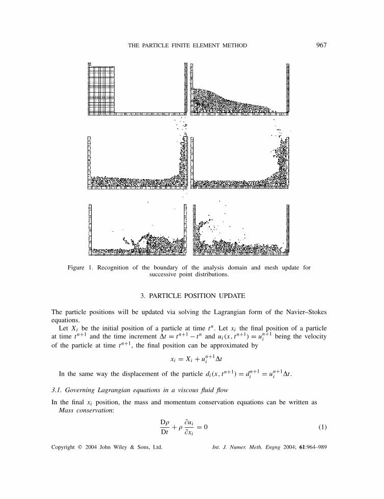
Finally, the most crucial characteristic of a Particle Method is that there is not a specifiedsolution domain. The problem domain is defined by the particle positions and hence, there isnot a boundary surface or line. This is the reason why, when a differential equation is to besolved in order to evaluate the forces, the boundary surface needs to be identified in order toimpose the boundary conditions. In addition, the particles can be used to generate a discretedomain within which the integral form of the governing differential equations is solved (seeFigure 1).

In this paper, a Particle Finite Element Method is proposed to deal with the incompressibleNavier–Stokes equations. Then, the true material will be continuous and incompressible whenit is submitted to compression forces, but with the possibility to separate under traction forces.This is the case of most physical fluids, like water, oils and other fluids with low rate ofsurface tractions.

Both, fluid and solid materials will be modelled by an arbitrary number of particles. Oneach particle the acting forces will be the gravity force (internal force of the particle) andthe interacting forces with the neighbour particles (external force to the particle). The externalforces will be evaluated solving the Navier–Stokes equations. For this reason a domain needsto be defined at each time step with a defined boundary surface where the boundary conditionswill be imposed. Also at each time step a new mesh is generated in order to define shapefunctions to solve the differential equations. This mesh is only useful for the definition of theinteracting forces and vanishes once the forces are evaluated (see Figure 1). The interpolationfunctions to be used are a particular case of the Finite Element Method shape functions.The boundary surface is defined using the Alpha-Shape Method explained in Section 4. Theevaluation of the interacting forces between particles is described next.



Figure 1. Recognition of the boundary of the analysis domain and mesh update forsuccessive point distributions.

3. PARTICLE POSITION UPDATE

The particle positions will be updated via solving the Lagrangian form of the Navier–Stokesequations.

Let Xi be the initial position of a particle at time tn. Let xi the final position of a particleat time tn+1 and the time increment �t = tn+1 − tn and ui(x, tn+1) = un+1

i being the velocityof the particle at time tn+1, the final position can be approximated by

xi = Xi + un+1i �t

In the same way the displacement of the particle di(x, tn+1) = dn+1i = un+1

i �t .

3.1. Governing Lagrangian equations in a viscous fluid flow

In the final xi position, the mass and momentum conservation equations can be written asMass conservation:

D�

Dt+ �

�ui

�xi

= 0 (1)



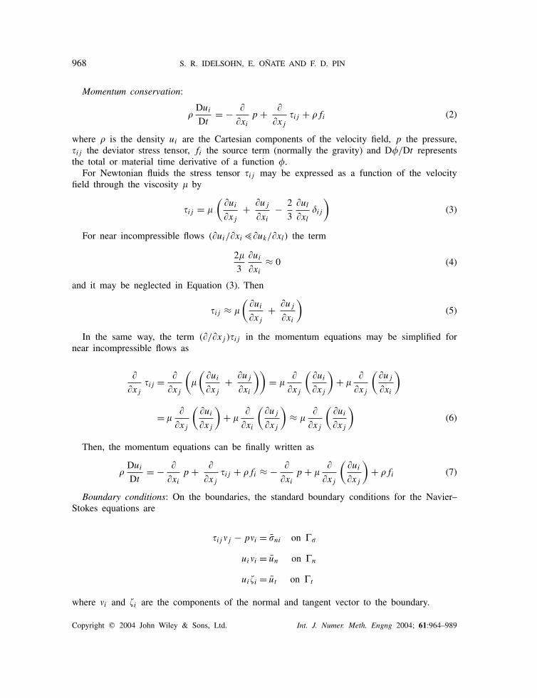
Momentum conservation:

�Dui

Dt= − �

�xi

p + ��xj

�ij + �fi (2)

where � is the density ui are the Cartesian components of the velocity field, p the pressure,�ij the deviator stress tensor, fi the source term (normally the gravity) and D�/Dt representsthe total or material time derivative of a function �.

For Newtonian fluids the stress tensor �ij may be expressed as a function of the velocityfield through the viscosity � by

�ij = �

(�ui

�xj

+ �uj

�xi

− 2

3

�ul

�xl

�ij

)(3)

For near incompressible flows (�ui/�xi>�uk/�xl) the term

2�

3

�ui

�xi

≈ 0 (4)

and it may be neglected in Equation (3). Then

�ij ≈ �

(�ui

�xj

+ �uj

�xi

)(5)

In the same way, the term (�/�xj )�ij in the momentum equations may be simplified fornear incompressible flows as

��xj

�ij = ��xj

(�

(�ui

�xj

+ �uj

�xi

))= �

��xj

(�ui

�xj

)+ �

��xj

(�uj

�xi

)

= ��

�xj

(�ui

�xj

)+ �

��xi

(�uj

�xj

)≈ �

��xj

(�ui

�xj

)(6)

Then, the momentum equations can be finally written as

�Dui

Dt= − �

�xi

p + ��xj

�ij + �fi ≈ − ��xi

p + ��

�xj

(�ui

�xj

)+ �fi (7)

Boundary conditions: On the boundaries, the standard boundary conditions for the Navier–Stokes equations are

�ij �j − p�i = �ni on ��

ui�i = un on �n

ui�i = ut on �t

where �i and �i are the components of the normal and tangent vector to the boundary.



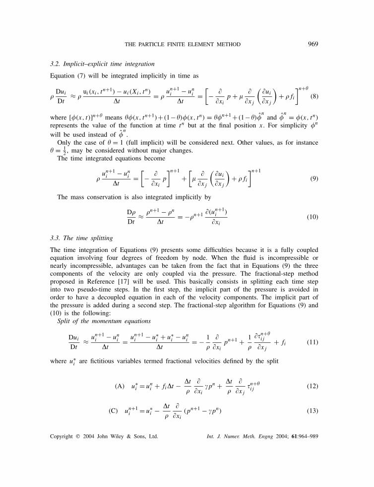
3.2. Implicit–explicit time integration

Equation (7) will be integrated implicitly in time as

�Dui

Dt≈ �

ui (xi, tn+1) − ui(Xi, t

n)

�t= �

un+1i − un

i

�t=[− �

�xi

p + ��

�xj

(�ui

�xj

)+ �fi

]n+

(8)

where [�(x, t)]n+ means �(x, tn+1)+(1−)�(x, tn) = �n+1 +(1−)�n

and �n = �(x, tn)

represents the value of the function at time tn but at the final position x. For simplicity �n

will be used instead of �n.

Only the case of = 1 (full implicit) will be considered next. Other values, as for instance = 1

2 , may be considered without major changes.The time integrated equations become

�un+1

i − uni

�t=[− �

�xi

p

]n+1

+[�

��xj

(�ui

�xj

)+ �fi

]n+1

(9)

The mass conservation is also integrated implicitly by

D�

Dt≈ �n+1 − �n

�t= −�n+1 �(un+1

i )

�xi

(10)

3.3. The time splitting

The time integration of Equations (9) presents some difficulties because it is a fully coupledequation involving four degrees of freedom by node. When the fluid is incompressible ornearly incompressible, advantages can be taken from the fact that in Equations (9) the threecomponents of the velocity are only coupled via the pressure. The fractional-step methodproposed in Reference [17] will be used. This basically consists in splitting each time stepinto two pseudo-time steps. In the first step, the implicit part of the pressure is avoided inorder to have a decoupled equation in each of the velocity components. The implicit part ofthe pressure is added during a second step. The fractional-step algorithm for Equations (9) and(10) is the following:

Split of the momentum equations

Dui

Dt≈ un+1

i − uni

�t= un+1

i − u∗i + u∗

i − uni

�t= − 1

�

��xi

pn+1 + 1

�

��n+ij

�xj

+ fi (11)

where u∗i are fictitious variables termed fractional velocities defined by the split

(A) u∗i = un

i + fi�t − �t

�

��xi

pn + �t

�

��xj

�n+ij (12)

(C) un+1i = u∗

i − �t

�

��xi

(pn+1 − pn) (13)



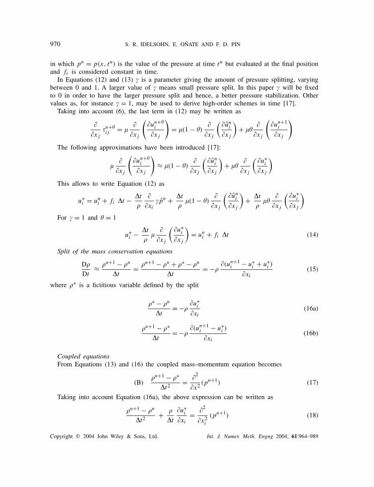
in which pn = p(x, tn) is the value of the pressure at time tn but evaluated at the final positionand fi is considered constant in time.

In Equations (12) and (13) is a parameter giving the amount of pressure splitting, varyingbetween 0 and 1. A larger value of means small pressure split. In this paper will be fixedto 0 in order to have the larger pressure split and hence, a better pressure stabilization. Othervalues as, for instance = 1, may be used to derive high-order schemes in time [17].

Taking into account (6), the last term in (12) may be written as

��xj

�n+ij = �

��xj

(�un+

i

�xj

)= �(1 − )

��xj

(�un

i

�xj

)+ �

��xj

(�un+1

i

�xj

)

The following approximations have been introduced [17]:

��

�xj

(�un+

i

�xj

)≈ �(1 − )

��xj

(�un

i

�xj

)+ �

��xj

(�u∗

i

�xj

)

This allows to write Equation (12) as

u∗i = un

i + fi �t − �t

�

��xi

pn + �t

��(1 − )

��xj

(�un

i

�xj

)+ �t

��

��xj

(�u∗

i

�xj

)

For = 1 and = 1

u∗i − �t

��

��xj

(�u∗

i

�xj

)= un

i + fi �t (14)

Split of the mass conservation equations

D�

Dt≈ �n+1 − �n

�t= �n+1 − �∗ + �∗ − �n

�t= −�

�(un+1i − u∗

i + u∗i )

�xi

(15)

where �∗ is a fictitious variable defined by the split

�∗ − �n

�t= −�

�u∗i

�xi

(16a)

�n+1 − �∗

�t= −�

�(un+1i − u∗

i )

�xi

(16b)

Coupled equationsFrom Equations (13) and (16) the coupled mass–momentum equation becomes

(B)�n+1 − �∗

�t2 = �2

�x2(pn+1) (17)

Taking into account Equation (16a), the above expression can be written as

�n+1 − �n

�t2 + �

�t

�u∗i

�xi

= �2

�x2i

(pn+1) (18)



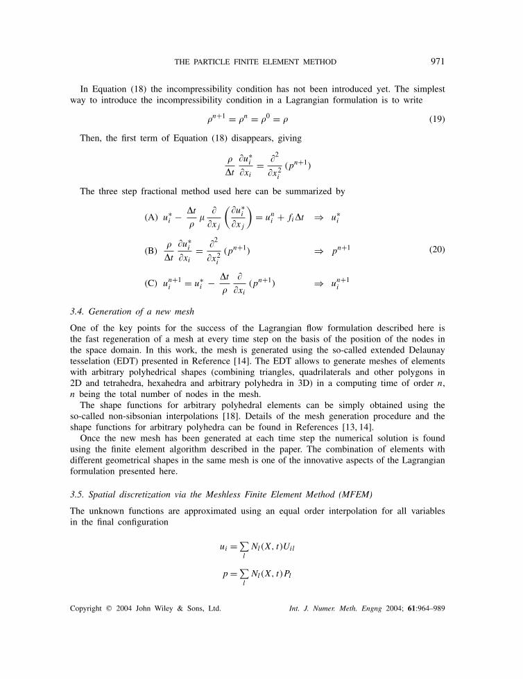
In Equation (18) the incompressibility condition has not been introduced yet. The simplestway to introduce the incompressibility condition in a Lagrangian formulation is to write

�n+1 = �n = �0 = � (19)

Then, the first term of Equation (18) disappears, giving

�

�t

�u∗i

�xi

= �2

�x2i

(pn+1)

The three step fractional method used here can be summarized by

(A) u∗i − �t

��

��xj

(�u∗

i

�xj

)= un

i + fi�t ⇒ u∗i

(B)�

�t

�u∗i

�xi

= �2

�x2i

(pn+1) ⇒ pn+1

(C) un+1i = u∗

i − �t

�

��xi

(pn+1) ⇒ un+1i

(20)

3.4. Generation of a new mesh

One of the key points for the success of the Lagrangian flow formulation described here isthe fast regeneration of a mesh at every time step on the basis of the position of the nodes inthe space domain. In this work, the mesh is generated using the so-called extended Delaunaytesselation (EDT) presented in Reference [14]. The EDT allows to generate meshes of elementswith arbitrary polyhedrical shapes (combining triangles, quadrilaterals and other polygons in2D and tetrahedra, hexahedra and arbitrary polyhedra in 3D) in a computing time of order n,n being the total number of nodes in the mesh.

The shape functions for arbitrary polyhedral elements can be simply obtained using theso-called non-sibsonian interpolations [18]. Details of the mesh generation procedure and theshape functions for arbitrary polyhedra can be found in References [13, 14].

Once the new mesh has been generated at each time step the numerical solution is foundusing the finite element algorithm described in the paper. The combination of elements withdifferent geometrical shapes in the same mesh is one of the innovative aspects of the Lagrangianformulation presented here.

3.5. Spatial discretization via the Meshless Finite Element Method (MFEM)

The unknown functions are approximated using an equal order interpolation for all variablesin the final configuration

ui =∑l

Nl(X, t)Uil

p =∑l

Nl(X, t)Pl



In matrix formui = NT(X, t)Ui

p = NT(X, t)P (21)

or in compact form

ui = NTi U =

NT

NT

NT

U (22)

where NT are the MFEM shape functions and U, P the nodal values of the three componentsof the unknown velocity and the pressure, respectively.

It must be noted that the shape functions N(X, t) are functions of the particle co-ordinates.Then, the shape functions may change in time following the particles position. During thetime step a mesh update may introduce change in the shape function definition which must betaken into account. During the time integration there are two times involved: tn and tn+1. Thefollowing notation will be used to distinguish between N(X, tn) and N(X, tn+1):

N(X, tn) = Nn and N(X, tn+1) = Nn+1 (23)

Nevertheless, the following hypothesis will be introduced: There is no mesh update duringeach time step. This means that if a mesh update is introduced at the beginning of a time step,the same mesh (but deformed) will be kept until the end of the time step.

Mathematically this means

N(X, tn) = N(X, tn+1) (24)

Unfortunately, this hypothesis is not always possible to satisfy for all meshes and thusintroduces small errors in the computation which are neglected in this paper.

Using the Galerkin weighted residual method to solve the split equations the followingintegrals must be written:

(A)

∫V

Niu∗i dV

�

�t−∫

V

Niuni dV

�

�t−∫

V

Nifi� dV +∫

V

Ni

��xi

pn dV

+∫

V

Ni��

�xj

{(�un+

i

�xj

)}dV −

∫��

Ni (�ni − (�n+ij �j − pn�i )) d� = 0

(25)

(B)

∫V

N

{�

�t

(�u∗

i

�xi

)− �2

�x2i

(pn+1 − pn)

}dV

+ �

�t

∫�u

N(un+1i �i − un+1

i �i ) d� = 0 (26)



(C)

∫V

Ni

{(un+1

i − u∗i )

�

�t+ �

�xi

(pn+1 − pn)

}dV

−∫

��

Ni (pn+1 − pn)�i d� = 0 (27)

where the boundary conditions have also been split and V is the volume at time tn+1.Integrating by parts some of the terms, the above equations become

(A)

∫V

Ni (u∗i − fi�t)

�

�tdV −

∫V

Niuni

�

�tdV +

∫V

Ni

��xi

pn dV

+ �∫

V

�Ni

�xj

�un+i

�xj

dV −∫

��Ni (�ni + pn�i ) d� = 0 (28)

(B) − �

�t

∫V

�N�xi

u∗i dV −

∫V

�N�xi

�(pn+1 − pn)

�xi

dV + �

�t

∫�u

Nun+1n d� = 0

(29)

(C)

∫V

Ni

{(un+1

i − u∗i )

�

�t+ �

�xi

(pn+1 − pn)

}dV −

∫��

Ni (pn+1 − pn)d� = 0

(30)

It must be noted that the essential and natural boundary conditions of Equations (29) are

p = 0 on �� (31)

un+1 · � = 0 on �u (32)

3.5.1. Discrete equations. Using approximations (22)–(24) the discrete equations become

(A)

∫V

NiNTi dV U∗

i =∫

V

NiNTi dV Un

i + �t

∫V

Nifi dV

− �t

�

∫V

Ni

�NT

�xi

dV Pn − �t�

�

∫V

�Ni

�xj

�NTi

�xj

dV Un+i

+ �t

�

∫��

Ni (�ni + pn) d� (33)

In compact form

MU∗ = MUn + �tF − �t

�BTPn − �t�

�KUn+



and making use of the approximation described before for Un+ϑ(M + �t�

�K)

U∗ = MUn + �tF − �t

�BTPn − �t�(1 − )

�KUn

and for = 1 and = 0

(A)

(M + �t�

�K)

U∗ = MUn + �tF (34)

In the same way

− �

�t

∫V

(�N�xi

NTi

)dV U∗ + �

�t

∫�u

Nun+1n d� = −

∫V

(�N�xi

�NT

�xi

)dV (Pn+1 − Pn)

(35)

In compact form

SPn+1 = �

�t(BU∗ − U) + SPn

and for = 1 and = 0

(B) SPn+1 = �

�t(BU∗ − U) (36)

Finally

∫V

NiNTi dV Un+1 =

∫V

NiNTi dV U∗ − �t

�

∫V

Ni

�NT

�xi

dV (Pn+1 − Pn)

+∫

��

NiNT d�(Pn+1 − Pn) (37)

In compact form

MUn+1 = MU∗ − �t

�BT(Pn+1 − Pn)

and for = 1 and = 0

(C) MUn+1 = MU∗ − �t

�BTPn+1 (38)

where the matrices are

M =

Mp 0 0

0 Mp 0

0 0 Mp

(39)



Mp =∫

V

NNT dV (40)

B =[∫

V

(�N�x

NT)

dV ;∫

V

(�N�y

NT)

dV ;∫

V

(�N�z

NT)

dV

](41)

S =∫

V

(�N�x

�NT

�x+ �N

�y

�NT

�y+ �N

�z

�NT

�z

)dV (42)

U =∫

�u

Nun+1n d� (43)

K =

S 0 0

0 S 0

0 0 S

(44)

FT =[∫

V

NTfx dV ;∫

V

NTfy dV ;∫

V

NTfz dV

]

+ 1

�

[∫��

NT�nx d�;∫

��

NT�ny d�;∫

��

NT�nz d�

](45)

3.6. Summary of a full iterative time step

A full time step may be described as follows: starting with the known values un and pn ineach particle, the computation of the new particle position involves the following steps:

(I) Approximate un+1 (For the first iteration un+1 = 0. For the subsequent iterationsthe value of un+1 corresponding to the last iteration is taken).

(II) Move the particles to the xn+1 position and generate a mesh.(III) Evaluate the u∗ velocity from (34). (It must be noted that the matrices M and

K are separated in 3 blocks. Then, this equations may be solved separately forU∗

x , U∗y and U∗

z . For �= 0 (implicit) involves the solution of 3 Laplacian equations.For = 0 (explicit) the M matrix may be lumped and inverted directly).

(IV) Evaluate the pressure pn+1 by solving the Laplacian Equation (36).(V) Evaluate the velocity un+1 using (38). Go to (I) until convergence.

The Lagrangian split scheme described has two important advantages:

(1) Step III is linear and may be explicit ( = 0) or implicit ( �= 0). The use of a Lagrangianformulation eliminates the standard convection terms present in Eulerian formulations. Theconvection terms are responsible for non-linearity, non-symmetry and non-self-adjoint op-erators which require the introduction of high-order stabilization terms to avoid numerical



oscillations. All these problems are not present in this formulation. Only the non-linearityremains due to the unknown of the final particle position.

(2) In all the steps, the system of equations to be solved are the evaluation of the velocitycomponents (step III) and the evaluation of the pressure (step IV). Those systems arescalar (only one degree of freedom by node), symmetric and positive definite. Then, itis very easy to solve them using a symmetric iterative scheme (such as the conjugategradient method).

3.7. Stabilization of the incompressibility condition

In the Eulerian form of the momentum equations, the discrete form must be stabilized inorder to avoid numerical wiggles in the velocity and pressure results. This is not the casein the Lagrangian formulation where no stabilization parameter must be added in Equations(34) and (38). Nevertheless, the incompressibility condition must be stabilized in equal-orderapproximations to avoid possible pressure oscillations in some particular cases.

For instance for small pressure split ( �= 0) or for small time step increments (Courantnumber much less than one) it is well known that the fractional step does not stabilize thepressure waves. In those particular cases, a stabilization term must be introduced in Equations(B) in order to eliminate pressure oscillations.

A simple and effective procedure to derive a stabilized formulation for incompressible flowsis based on the so-called Finite Calculus formulations [19–21].

In all the examples presented in this paper, the parameter was always fixed equal to zeroand the time increments were fixed to a given value of the Courant number ≈ 1, avoiding inthis way all the stabilization problems.

4. BOUNDARY SURFACES RECOGNITION

One of the main problems in mesh generation is the correct definition of the boundary domain.Sometimes, boundary nodes are explicitly defined as special nodes, which are different frominternal nodes. In other cases, the total set of nodes is the only information available andthe algorithm must recognize the boundary nodes. Such is the case in Particle Methods inwhich, at each time step, a new particle position is obtained and the boundary-surface must berecognized using the new particle positions.

The use of the MFEM with the extended Delaunay partition makes it easier to recognizeboundary nodes.

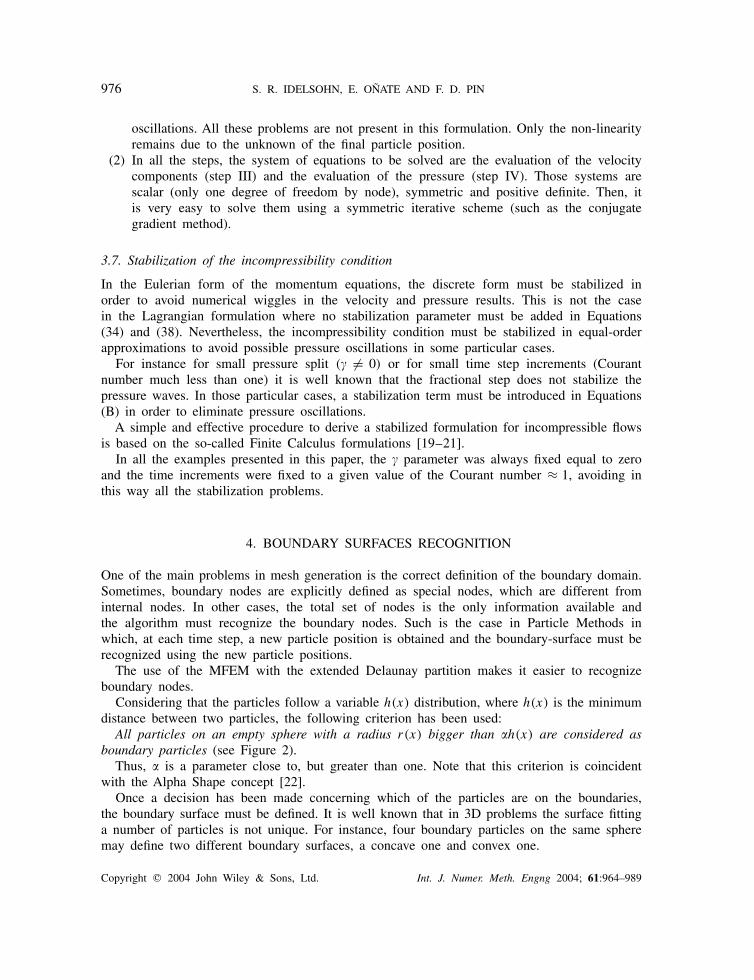
Considering that the particles follow a variable h(x) distribution, where h(x) is the minimumdistance between two particles, the following criterion has been used:

All particles on an empty sphere with a radius r(x) bigger than �h(x) are considered asboundary particles (see Figure 2).

Thus, � is a parameter close to, but greater than one. Note that this criterion is coincidentwith the Alpha Shape concept [22].

Once a decision has been made concerning which of the particles are on the boundaries,the boundary surface must be defined. It is well known that in 3D problems the surface fittinga number of particles is not unique. For instance, four boundary particles on the same spheremay define two different boundary surfaces, a concave one and convex one.



Figure 2. Contour recognition: Empty circles with radius � h(x) define the boundary particles.

In this work, the boundary surface is defined with all the polyhedral surfaces having all theirparticles on the boundary and belonging to just one polyhedron. See Reference [13].

The correct boundary surface may be important to define the correct normal external to thesurface. Furthermore, in weak forms (Galerkin) a correct evaluation of the volume domain isalso important. Nevertheless, it must be noted that in the criterion proposed above, the errorin the boundary surface definition is proportional to h. This is the error order accepted in anumerical method for a given node distribution. The only way to obtain more accurate boundarysurface definition is by decreasing the distance between the particles.

5. NUMERICAL RESULTS

A number of free-surface flow and fluid–structure interaction problems will be presented. In afirst group of examples the interacting solid will be considered infinitely rigid and fixed. Thosecases are useful to compare the results with experimental and analytical ones. The interactingsolid will also be represented with particles but with imposed velocity equal to zero. In asecond group of examples moving rigid solid motions will be considered. In all cases, theelastic strains will be neglected. The solid will be considered in two different ways:

(a) As a particular material with a high viscosity parameter, much higher than the fluiddomain. For practical purposes a 1010� value will be considered. This value is enoughto represent a solid without introducing numerical problems.

(b) The solid will be considered as a boundary contour with an imposed velocity. After eachtime step, the fluid forces on the solid due to the pressure and the viscous terms will beevaluated. In the next step, the solid will move rigidly using Newton law.

Time stepping and iterative process: The time step length �t was imposed to a variablevalue and evaluated at the beginning of each time step. The criterion to calculate the time step



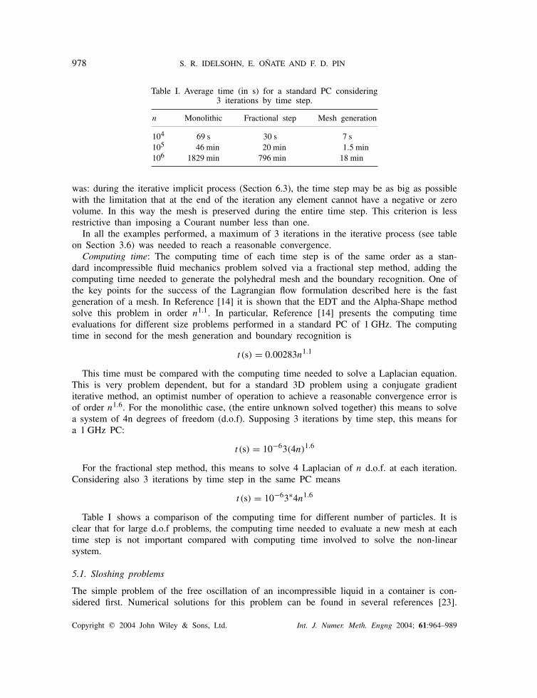
Table I. Average time (in s) for a standard PC considering3 iterations by time step.

n Monolithic Fractional step Mesh generation

104 69 s 30 s 7 s105 46 min 20 min 1.5 min106 1829 min 796 min 18 min

was: during the iterative implicit process (Section 6.3), the time step may be as big as possiblewith the limitation that at the end of the iteration any element cannot have a negative or zerovolume. In this way the mesh is preserved during the entire time step. This criterion is lessrestrictive than imposing a Courant number less than one.

In all the examples performed, a maximum of 3 iterations in the iterative process (see tableon Section 3.6) was needed to reach a reasonable convergence.

Computing time: The computing time of each time step is of the same order as a stan-dard incompressible fluid mechanics problem solved via a fractional step method, adding thecomputing time needed to generate the polyhedral mesh and the boundary recognition. One ofthe key points for the success of the Lagrangian flow formulation described here is the fastgeneration of a mesh. In Reference [14] it is shown that the EDT and the Alpha-Shape methodsolve this problem in order n1.1. In particular, Reference [14] presents the computing timeevaluations for different size problems performed in a standard PC of 1 GHz. The computingtime in second for the mesh generation and boundary recognition is

t (s) = 0.00283n1.1

This time must be compared with the computing time needed to solve a Laplacian equation.This is very problem dependent, but for a standard 3D problem using a conjugate gradientiterative method, an optimist number of operation to achieve a reasonable convergence error isof order n1.6. For the monolithic case, (the entire unknown solved together) this means to solvea system of 4n degrees of freedom (d.o.f). Supposing 3 iterations by time step, this means fora 1 GHz PC:

t (s) = 10−63(4n)1.6

For the fractional step method, this means to solve 4 Laplacian of n d.o.f. at each iteration.Considering also 3 iterations by time step in the same PC means

t (s) = 10−63∗4n1.6

Table I shows a comparison of the computing time for different number of particles. It isclear that for large d.o.f problems, the computing time needed to evaluate a new mesh at eachtime step is not important compared with computing time involved to solve the non-linearsystem.

5.1. Sloshing problems

The simple problem of the free oscillation of an incompressible liquid in a container is con-sidered first. Numerical solutions for this problem can be found in several references [23].



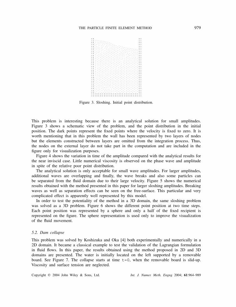
Figure 3. Sloshing. Initial point distribution.

This problem is interesting because there is an analytical solution for small amplitudes.Figure 3 shows a schematic view of the problem, and the point distribution in the initialposition. The dark points represent the fixed points where the velocity is fixed to zero. It isworth mentioning that in this problem the wall has been represented by two layers of nodesbut the elements constructed between layers are omitted from the integration process. Thus,the nodes on the external layer do not take part in the computation and are included in thefigure only for visualization purposes.

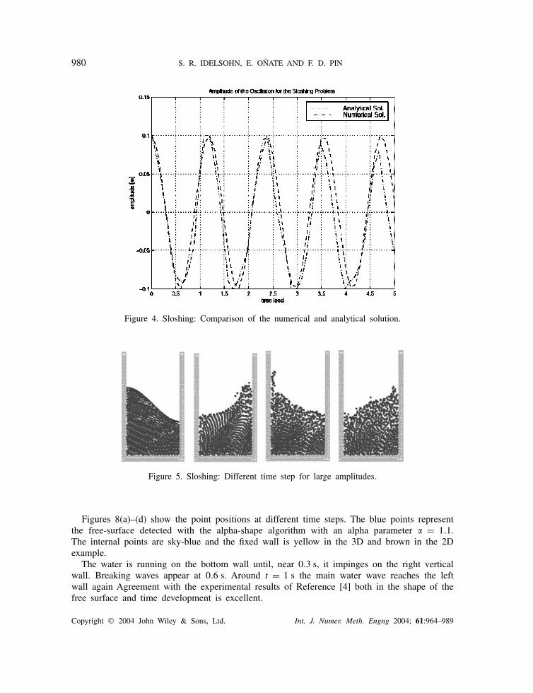
Figure 4 shows the variation in time of the amplitude compared with the analytical results forthe near inviscid case. Little numerical viscosity is observed on the phase wave and amplitudein spite of the relative poor point distribution.

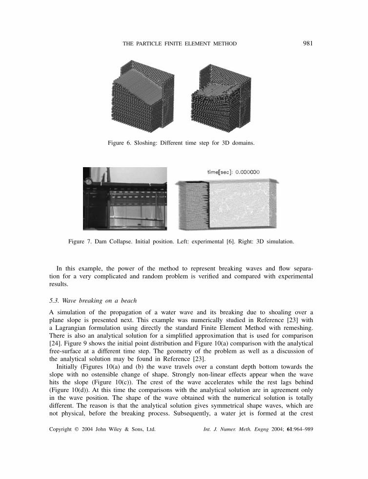
The analytical solution is only acceptable for small wave amplitudes. For larger amplitudes,additional waves are overlapping and finally, the wave breaks and also some particles canbe separated from the fluid domain due to their large velocity. Figure 5 shows the numericalresults obtained with the method presented in this paper for larger sloshing amplitudes. Breakingwaves as well as separation effects can be seen on the free-surface. This particular and verycomplicated effect is apparently well represented by this model.

In order to test the potentiality of the method in a 3D domain, the same sloshing problemwas solved as a 3D problem. Figure 6 shows the different point position at two time steps.Each point position was represented by a sphere and only a half of the fixed recipient isrepresented on the figure. The sphere representation is used only to improve the visualizationof the fluid movement.

5.2. Dam collapse

This problem was solved by Koshizuka and Oka [4] both experimentally and numerically in a2D domain. It became a classical example to test the validation of the Lagrangian formulationin fluid flows. In this paper, the results obtained using the method proposed in 2D and 3Ddomains are presented. The water is initially located on the left supported by a removableboard. See Figure 7. The collapse starts at time t=0, when the removable board is slid-up.Viscosity and surface tension are neglected.



Figure 4. Sloshing: Comparison of the numerical and analytical solution.

Figure 5. Sloshing: Different time step for large amplitudes.

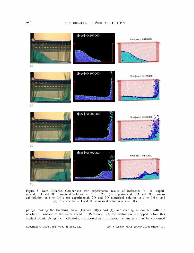
Figures 8(a)–(d) show the point positions at different time steps. The blue points representthe free-surface detected with the alpha-shape algorithm with an alpha parameter � = 1.1.The internal points are sky-blue and the fixed wall is yellow in the 3D and brown in the 2Dexample.

The water is running on the bottom wall until, near 0.3 s, it impinges on the right verticalwall. Breaking waves appear at 0.6 s. Around t = 1 s the main water wave reaches the leftwall again Agreement with the experimental results of Reference [4] both in the shape of thefree surface and time development is excellent.



Figure 6. Sloshing: Different time step for 3D domains.

Figure 7. Dam Collapse. Initial position. Left: experimental [6]. Right: 3D simulation.

In this example, the power of the method to represent breaking waves and flow separa-tion for a very complicated and random problem is verified and compared with experimentalresults.

5.3. Wave breaking on a beach

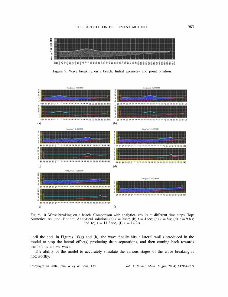
A simulation of the propagation of a water wave and its breaking due to shoaling over aplane slope is presented next. This example was numerically studied in Reference [23] witha Lagrangian formulation using directly the standard Finite Element Method with remeshing.There is also an analytical solution for a simplified approximation that is used for comparison[24]. Figure 9 shows the initial point distribution and Figure 10(a) comparison with the analyticalfree-surface at a different time step. The geometry of the problem as well as a discussion ofthe analytical solution may be found in Reference [23].

Initially (Figures 10(a) and (b) the wave travels over a constant depth bottom towards theslope with no ostensible change of shape. Strongly non-linear effects appear when the wavehits the slope (Figure 10(c)). The crest of the wave accelerates while the rest lags behind(Figure 10(d)). At this time the comparisons with the analytical solution are in agreement onlyin the wave position. The shape of the wave obtained with the numerical solution is totallydifferent. The reason is that the analytical solution gives symmetrical shape waves, which arenot physical, before the breaking process. Subsequently, a water jet is formed at the crest



Figure 8. Dam Collapse. Comparison with experimental results of Reference [6]: (a) experi-mental, 2D and 3D numerical solution at t = 0.2 s; (b) experimental, 2D and 3D numeri-cal solution at t = 0.4 s; (c) experimental, 2D and 3D numerical solution at t = 0.6 s; and

(d) experimental, 2D and 3D numerical solution at t = 0.8 s.

plunge making the breaking wave (Figures 10(e) and (f)) and coming in contact with thenearly still surface of the water ahead. In Reference [23] the evaluation is stopped before thiscontact point. Using the methodology proposed in this paper, the analysis may be continued



Figure 9. Wave breaking on a beach. Initial geometry and point position.

Figure 10. Wave breaking on a beach. Comparison with analytical results at different time steps. Top:Numerical solution. Bottom: Analytical solution: (a) t = 0 sec; (b) t = 4 sec; (c) t = 8 s; (d) t = 9.8 s;

and (e) t = 11.2 sec, (f) t = 14.2 s.

until the end. In Figures 10(g) and (h), the wave finally hits a lateral wall (introduced in themodel to stop the lateral effects) producing drop separations, and then coming back towardsthe left as a new wave.

The ability of the model to accurately simulate the various stages of the wave breaking isnoteworthy.



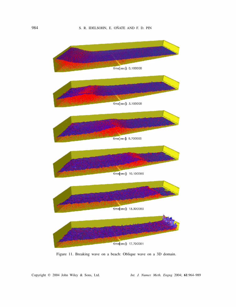
Figure 11. Breaking wave on a beach: Oblique wave on a 3D domain.



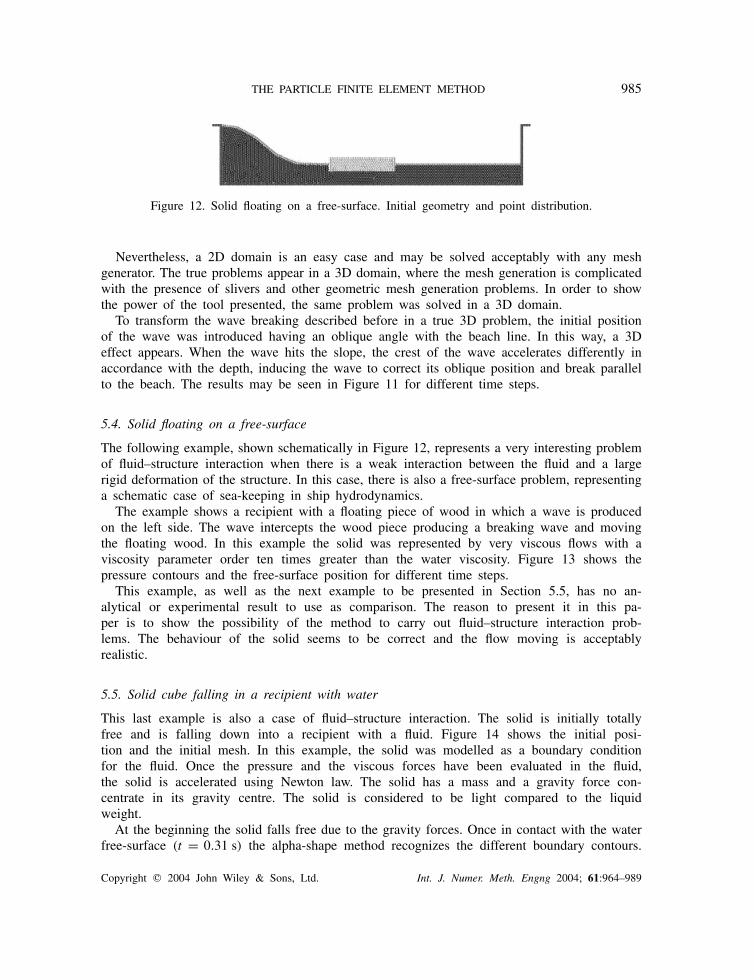
Figure 12. Solid floating on a free-surface. Initial geometry and point distribution.

Nevertheless, a 2D domain is an easy case and may be solved acceptably with any meshgenerator. The true problems appear in a 3D domain, where the mesh generation is complicatedwith the presence of slivers and other geometric mesh generation problems. In order to showthe power of the tool presented, the same problem was solved in a 3D domain.

To transform the wave breaking described before in a true 3D problem, the initial positionof the wave was introduced having an oblique angle with the beach line. In this way, a 3Deffect appears. When the wave hits the slope, the crest of the wave accelerates differently inaccordance with the depth, inducing the wave to correct its oblique position and break parallelto the beach. The results may be seen in Figure 11 for different time steps.

5.4. Solid floating on a free-surface

The following example, shown schematically in Figure 12, represents a very interesting problemof fluid–structure interaction when there is a weak interaction between the fluid and a largerigid deformation of the structure. In this case, there is also a free-surface problem, representinga schematic case of sea-keeping in ship hydrodynamics.

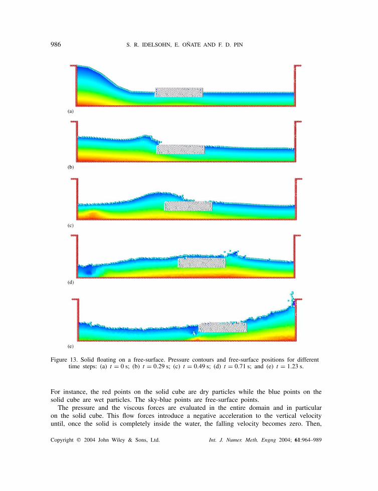
The example shows a recipient with a floating piece of wood in which a wave is producedon the left side. The wave intercepts the wood piece producing a breaking wave and movingthe floating wood. In this example the solid was represented by very viscous flows with aviscosity parameter order ten times greater than the water viscosity. Figure 13 shows thepressure contours and the free-surface position for different time steps.

This example, as well as the next example to be presented in Section 5.5, has no an-alytical or experimental result to use as comparison. The reason to present it in this pa-per is to show the possibility of the method to carry out fluid–structure interaction prob-lems. The behaviour of the solid seems to be correct and the flow moving is acceptablyrealistic.

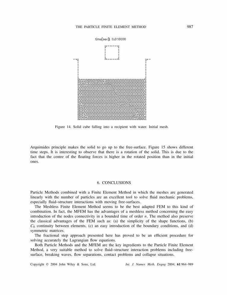
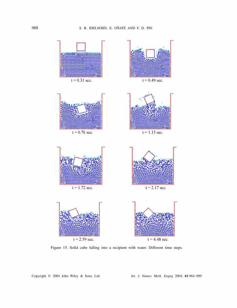
5.5. Solid cube falling in a recipient with water

This last example is also a case of fluid–structure interaction. The solid is initially totallyfree and is falling down into a recipient with a fluid. Figure 14 shows the initial posi-tion and the initial mesh. In this example, the solid was modelled as a boundary conditionfor the fluid. Once the pressure and the viscous forces have been evaluated in the fluid,the solid is accelerated using Newton law. The solid has a mass and a gravity force con-centrate in its gravity centre. The solid is considered to be light compared to the liquidweight.

At the beginning the solid falls free due to the gravity forces. Once in contact with the waterfree-surface (t = 0.31 s) the alpha-shape method recognizes the different boundary contours.



Figure 13. Solid floating on a free-surface. Pressure contours and free-surface positions for differenttime steps: (a) t = 0 s; (b) t = 0.29 s; (c) t = 0.49 s; (d) t = 0.71 s; and (e) t = 1.23 s.

For instance, the red points on the solid cube are dry particles while the blue points on thesolid cube are wet particles. The sky-blue points are free-surface points.

The pressure and the viscous forces are evaluated in the entire domain and in particularon the solid cube. This flow forces introduce a negative acceleration to the vertical velocityuntil, once the solid is completely inside the water, the falling velocity becomes zero. Then,



Figure 14. Solid cube falling into a recipient with water. Initial mesh.

Arquimides principle makes the solid to go up to the free-surface. Figure 15 shows differenttime steps. It is interesting to observe that there is a rotation of the solid. This is due to thefact that the centre of the floating forces is higher in the rotated position than in the initialones.

6. CONCLUSIONS

Particle Methods combined with a Finite Element Method in which the meshes are generatedlinearly with the number of particles are an excellent tool to solve fluid mechanic problems,especially fluid–structure interactions with moving free-surfaces.

The Meshless Finite Element Method seems to be the best adapted FEM to this kind ofcombination. In fact, the MFEM has the advantages of a meshless method concerning the easyintroduction of the nodes connectivity in a bounded time of order n. The method also preservethe classical advantages of the FEM such as: (a) the simplicity of the shape functions, (b)C0 continuity between elements, (c) an easy introduction of the boundary conditions, and (d)symmetric matrices.

The fractional step approach presented here has proved to be an efficient procedure forsolving accurately the Lagrangian flow equations.

Both Particle Methods and the MFEM are the key ingredients to the Particle Finite ElementMethod, a very suitable method to solve fluid–structure interaction problems including free-surface, breaking waves, flow separations, contact problems and collapse situations.



Figure 15. Solid cube falling into a recipient with water. Different time steps.



REFERENCES

1. Gingold RA, Monaghan JJ. Smoothed particle hydrodynamics, theory and application to non-spherical stars.Monthly Notices of the Royal Astronomical Society 1997; 181:375–389.

2. Bonet J, Kulasegaram S. Correction and stabilization of smooth particle hydrodynamics methods withapplications in metal forming simulation. International Journal for Numerical Methods in Engineering2000;47:1189–1214.

3. Dilts GA. Moving least squares particle hydrodynamics. I. Consistency and stability. International Journalfor Numerical Methods in Engineering 1999; 44:1115–1155.

4. Koshizuka S, Oka Y. Moving particle semi-implicit method for fragmentation of incompressible fluid. NuclearEngineering Science 1996; 123:421–434.

5. Crowley WP. Lecture Notes in Physics. Springer: Berlin, 1970; 8–37.6. Fritts MJ, Crowley WP, Trease HE. The Free Lagrange Method, Lecture Notes in Physics, vol. 238. Springer:

New York, 1985.7. Belytschko T, Liu Y, Gu L. Element free Galerkin methods. International Journal for Numerical Methods

in Engineering 1994; 37:229–256.8. De S, Bathe KJ. The method of finite spheres with improved numerical integration. Computers and Structures

2001; 79:2183–2196.9. Nayroles B, Touzot G, Villon P. Generalizing the fem: diffuse approximation and diffuse elements.

Computational Mechanics 1992; 10:307–318.10. Oñate E, Idelsohn SR, Zienkiewicz OC, Taylor RL. A finite point method in computational mechanics.

Applications to convective transport and fluid flow. International Journal for Numerical Methods inEngineering 1996; 39(22):3839–3886.

11. Oñate E, Idelsohn SR, Zienkiewicz OC, Taylor RL, Sacco C. A stabilized finite point method for analysisof fluid mechanics problems. Computer Methods in Applied Mechanics and Engineering 1996; 39:315–346.

12. Idelsohn SR, Storti MA, Oñate E. Lagrangian formulations to solve free surface incompressible inviscidfluid flows. Computer Methods in Applied Mechanics and Engineering 2001; 191:583–593.

13. Idelsohn SR, Oñate E, Calvo N, Del Pin F. The meshless finite element method. International Journal forNumerical Methods in Engineering 2003; 58(6):893–912.

14. Calvo N, Idelsohn SR, Oñate E. Polyhedrization of an arbitrary 3D point set. Computer Method in AppliedMechanics and Engineering 2003; 192:2649–2667.

15. Rojek J, Oñate E, Zarate F, Miquel J. Modelling of rock, soil and granular materials using sphericalelements. Proceedings of the European Conference on Computer Mechanics (ECCM 2001), Cracow, Poland,June 2001.

16. Idelsohn SR, Oñate E, Del Pin F. A Lagrangian meshless finite element method applied to fluid–structureinteraction problems. Computer and Structures 2003; 81:655–671.

17. Codina R. Pressure stability in fractional step finite element methods for incompressible flows. Journal ofComputational Physics 2001; 170:112–140.

18. Belikov V, Semenov A. Non-sibsonian interpolation on arbitrary system of points in Euclidean spaceand adaptive generating isolines algorithm. Numerical Grid Generation in Computational Field Simulation,Proceedings of the 6th International Conference. Greenwich University, July 1998.

19. Oñate E. Derivation of stabilized equations for advective–diffusive transport and fluid flow problems. ComputerMethods in Applied Mechanics and Engineering 1998; 151(1–2):233–267.

20. Oñate E. A stabilized finite element method for incompressible viscous flows using a finite increment calculusformulation. Computer Methods in Applied Mechanics and Engineering 2002; 182(1–2):355–370.

21. Oñate E. Possibilities of finite calculus in computational mechanics. International Journal for NumericalMethods in Engineering 2004; 60:255–281.

22. Edelsbrunner H, Mucke EP. Three-dimensional alpha-shape. ACM Transactions on Graphics 1994; 3:43–72.23. Radovitzky R, Ortiz M. Lagrangian finite element analysis of a Newtonian flows. International Journal for

Numerical Methods in Engineering 1998; 43:607–619.24. Laitone EV. The second approximation to cnoidal waves. Journal of Fluid Mechanics 1960; 9:430.


the particle finite element method: a powerful tool to ... · the particle ﬁnite element method:...

Documents