Applied Mathematics, 2014, 5, 3328-3334 Published Online December 2014 in SciRes. http://www.scirp.org/journal/am http://dx.doi.org/10.4236/am.2014.521310

How to cite this paper: Abo Essa, Y.M., Abouefarag, I. and Rahmo, E.-D. (2014) The Numerical Solution of the MRLW Equa-tion Using the Multigrid Method. Applied Mathematics, 5, 3328-3334. http://dx.doi.org/10.4236/am.2014.521310

The Numerical Solution of the MRLW Equation Using the Multigrid Method Yasser Mohamed Abo Essa1,2, Ibrahim Abouefarag1,3, El-Desouky Rahmo1,4

1Mathematics Department, Faculty of Education and Science (AL-Khurmah Branch), Taif University, Taif, KSA 2Mathematics Department, Faculty of Science, Al-Azhar University, Nasr City, Cairo, Egypt 3Mathematics Department, Faculty of Science, Suez Canal University, Ismailia, Egypt 4Mathematics Department, Faculty of Science, Mansoura University, Mansoura, Egypt Email: dd_yasser@yahoo.com, iabouelfarag@hotmail.com, desoukyr@hotmail.com Received 29 September 2014; revised 25 October 2014; accepted 10 November 2014

Copyright © 2014 by authors and Scientific Research Publishing Inc. This work is licensed under the Creative Commons Attribution International License (CC BY). http://creativecommons.org/licenses/by/4.0/

Abstract In this paper, we obtained the numerical solutions of the modified regularized long-wave (MRLW) equation t x x xxtu u u u μu2 0+ + − =α , by using the multigrid method and finite difference method. The solitary wave motion, interaction of two and three solitary waves, and development of the Maxwellian initial condition into solitary waves are studied using the proposed method. The nu-merical solutions are compared with the known analytical solutions. Using L L2 , ∞ error norms and conservative properties of mass, momentum and energy, accuracy and efficiency of the men-tioned method will be established through comparison with other techniques.

Keywords Multigrid Method, Finite Difference Method, MRLW Equation

1. Introduction The numerical solution of partial differential equations requires some discretization of the domain into a collec-tion of points. A large system of equations comes out from discretization of the same partial differential equa-tions and the optimal method for solving these problems is multigrid method, see [1]-[9].

Consider the following one-dimensional modified regularized long-wave (MRLW) equation: equation: 2 0,t x x xxtu u u u uα µ+ + − = (1)

where t is the time, x is the space coordinate, ,α µ are positive constants and u is the wave amplitude with the physical boundary conditions 0u → as x → ±∞ . This equation was first introduced to describe the

Y. M. Abo Essa et al.

3329

development of an undular bore by Peregrine [10] and later by Benjamin et al. [11]. Equation (1) has various applications as in physics media since it describes the phenomena with weak nonlinearity and dispersion waves, including nonlinear transverse waves in shallow water, ion-acoustic and magneto hydrodynamic waves in plas-ma, and phonon packets in nonlinear crystals [11].

Although the analytical solutions of the MRLW equation, with a limited set of boundary and initial conditions, have been existed, many authors are recently interested in the numerical solutions of this equation. Gardner et al. [12] introduced a collocation solution to the MRLW equation using quintic B-spline finite elements. Khalifa et al. [13] [14] applied the finite difference and cubic B-spline collocation finite element method to obtain the nu-merical solutions of the MRLW equation. Solutions based on collocation method with quadratic B-spline finite elements and the central finite difference method for time are investigated by Raslan [15]. Raslan and Hassan [16] solved the MRLW equation by a collocation finite element method using quadratic, cubic, quartic, and quintic B-spline to obtain the numerical solutions of the single solitary wave. Ali [17] has formulated a classical radial basis function collocation method for solving the MRLW equation. Haq et al. [18] have developed a nu-merical scheme based on quartic B-spline collocation method for the numerical solution of MRLW equation. Karakoc and Geyikli [19] solved the MRLW equation by using the Petrov-Galerkin finite element method.

An outline of this paper is as follows: we begin in Section 2 by reviewing the analytical solution of the MRLW equation. In Section 3, we derive a new numerical method based on the multigrid technique and finite difference method for obtaining the numerical solution of MRLW equation. Finally, in Section 4, we introduce the numerical results for solving the MRLW equation through some well known standard problems.

2. The Analytical Solution The exact solution of Equation (1) can be written in the form [12] [14]:

( ) ( )( )( )0

6, sech 1 ,cu x t P x c t xα

= − + − (2)

which represents the motion of a single solitary wave with amplitude c , where ( ) 0,

1cP xcµ

=+

and c

are arbitrary constants. The initial condition is given by

( ) ( )( )06,0 sech .cu x P x xα

= − (3)

The conservation properties of the MRLW equation related to mass, momentum and energy are determined by following three invariants on the region a x b≤ ≤ :

( )2 2 4 21 2 3

6d , d , d .b b b

x xa a a

I u x I u u x I u u xµ µα

= = + = − ∫ ∫ ∫ (4)

3. Numerical Method The basic idea of multigrid techniques is illustrated by Brandt [1]. In this section we apply this method for initial boundary value problem, except that, the upper boundary conditions change with time, in which the initial con-dition is ( ) ( ),0u x f x= for 0 t T< < . Dividing the interval of time to K parts, we obtain the solutions of the partial differential equation at time t1 and use these solutions as initial values for the next level ( ) ( )1,0 ,u x u x t= , and for the other, we obtain the solutions at time T . The numbers of points in a coarse grid for this domain are two points. We apply the full multigrid algorithm for the MRLW equation. Assuming the initial condition ( ) ( ),0u x f x= and the solution ( ),u x t , ,0a x b t T≤ ≤ ≤ ≤ has the usual partition with a space step size x∆ and a time step size t∆ ( )1 , 0,1, 2,K Kt t t K+ = + ∆ = . We start handling the non-linear term 2

xu u by ex-

pressing in the form 31

3ux

∂∂

. The back-time and centre-space difference for Equation (1) is

( ) ( ) ( ) ( ) ( )( ) ( )

3 3

1, 1, 1, 1, 1 , , 1 1, 1, 1, , 1 1, 1,2

20,

2 6

k k k k k k k kk k k ki n i n i n i n i n i n i n i ni n i n i n i n u u u u u u u uu u u u

t x x x tα µ+ − + + − − − − −− + −

− − − − + −− −+ + − =

∆ ∆ ∆ ∆ ∆ (5)

Y. M. Abo Essa et al.

3330

where 1, , 2 1, 1, , 2k ki n= − = , 1, ,k M= for a set grids 1 2, , , .MG G G Step 1: ( ) ( )0, ,0 .K u x f x= = Step 2: Starting from 1k = in the coarse grid, we can calculate the approximate value ,i nu at two points

using Equation (5) leading to:

( )( ) ( )( )( ) ( )( )( )

( )( ) ( ) ( )( ) ( )( )( )

1 1 1, 1, 1,2

3 3 21 1 11, 1, , 1

1 11, 1 1, 1

1 2 22 4

2 43

2 ; 1, 1,2.

i n i n i n

i n i n i n

i n i n

u x t u x t ux

x t u u x u

u u i n

µ µµ

α µ

µ

+ −

+ − −

+ − − −

= − ∆ ∆ + ∆ ∆ +∆ +

− ∆ ∆ − + ∆ +

− + = =

(6)

The right hand side for the last equation can be computed using the initial and boundary conditions. Step 3: Interpolating the grid functions from the coarse grid to fine grid using linear interpolation 1k

kI + , in which

1 1 ,k k kku I u+ += (7)

that can be written explicitly as:

( )( )

( )

12 ,2 ,

12 1,2 , 1,

12 ,2 1 , , 1

12 1,2 1 , 1, , 1 1, 1

; 1, , 2 1, 1, , 2 ,

0.5 ; 0, , 2 1, 1, , 2 ,

0.5 ; 1, , 2 1, 0, , 2 1,

0.25 ; , 0, , 2 1.

k k k ki n i n

k k k k ki n i n i n

k k k k ki n i n i n

k k k k k ki n i n i n i n i n

u u i n

u u u i n

u u u i n

u u u u u i n

+

++ +

++ +

++ + + + + +

= = − =

= + = − =

= + = − = −

= + + + = −

(8)

Step 4: Doing relaxation sweep on 1kG + using the point relaxation

( )( ) ( )( )( ) ( )( )( )

( )( ) ( ) ( )( ) ( )( )( )

1, 1, 1,2

3 3 21, 1, , 1

1 11, 1 1, 1

1 2 22 4

2 432 ; 1, , 2 1, 1, , 2 .

k k ki n i n i n

k k ki n i n i n

k k k ki n i n

u x t u x t ux

x t u u x u

u u i n

µ µµ

α µ

µ

++ −

+ − −

+ ++ − − −

= − ∆ ∆ + ∆ ∆ +∆ +

− ∆ ∆ − + ∆ +

− + = − =

(9)

Step 5: Computing the residuals 1kr + on 1kG + and inject them into kG using full weighting restriction 1

kkI + to get kr as:

11 ,k k k

kr I r ++= (10)

( )

1 1 1 1, 2 1,2 1 2 1,2 1 2 1,2 1 2 1,2 1

1 1 1 1 12 ,2 1 2 ,2 1 2 1,2 2 1,2 2 ,2

116

2 4 ; , 1, , 2 1.

k k k k ki n i n i n i n i n

k k k k k ki n i n i n i n i n

r r r r r

r r r r r i n

+ + + +− − − + + − + +

+ + + + +− + − +

= + + +

+ + + + + = −

(11)

Step 6: Computing an approximate solution of error ek . Step 7: Interpolating the solution of error ek onto 1kG + , 1 1e e ,k k k

kI+ += and adding it to 1ku + which is the approximate value of u on the fine grid with 2k = .

By taking this solution on coarse grid and repeating steps 3 - 7, we obtain the approximate values of u on the grid with 3k = and so 4,5, ,k M= the final value is the solution at the time level 1K + .

Step 8: 1K K= + , go to step 2 (lead to the solution at higher time level as needed).

4. Numerical Results In this section, numerical solutions of MRLW equation are obtained for standard problems as: the motion of

Y. M. Abo Essa et al.

3331

single solitary wave, interaction of two and three solitary waves and development of Maxwellian initial condi-tion into solitary waves. 2L and L∞ error norms are used to show how good the numerical results in compar-ison with the exact results.

4.1. The Motion of Single Solitary Wave Consider equation (1) with boundary conditions

( ) ( )( ) ( )

, 0, , 0,

, 0, , 0, 0,x x

u a t u b t

u a t u b t t

= =

= = > (12)

and the initial condition (4). The analytical values of the invariants of this problem can be found as [12]:

2

1 2 3π 2 2 4 2, , .

3 3 3c c Pc c PcI I I

P P Pµ µ

= = + = − (13)

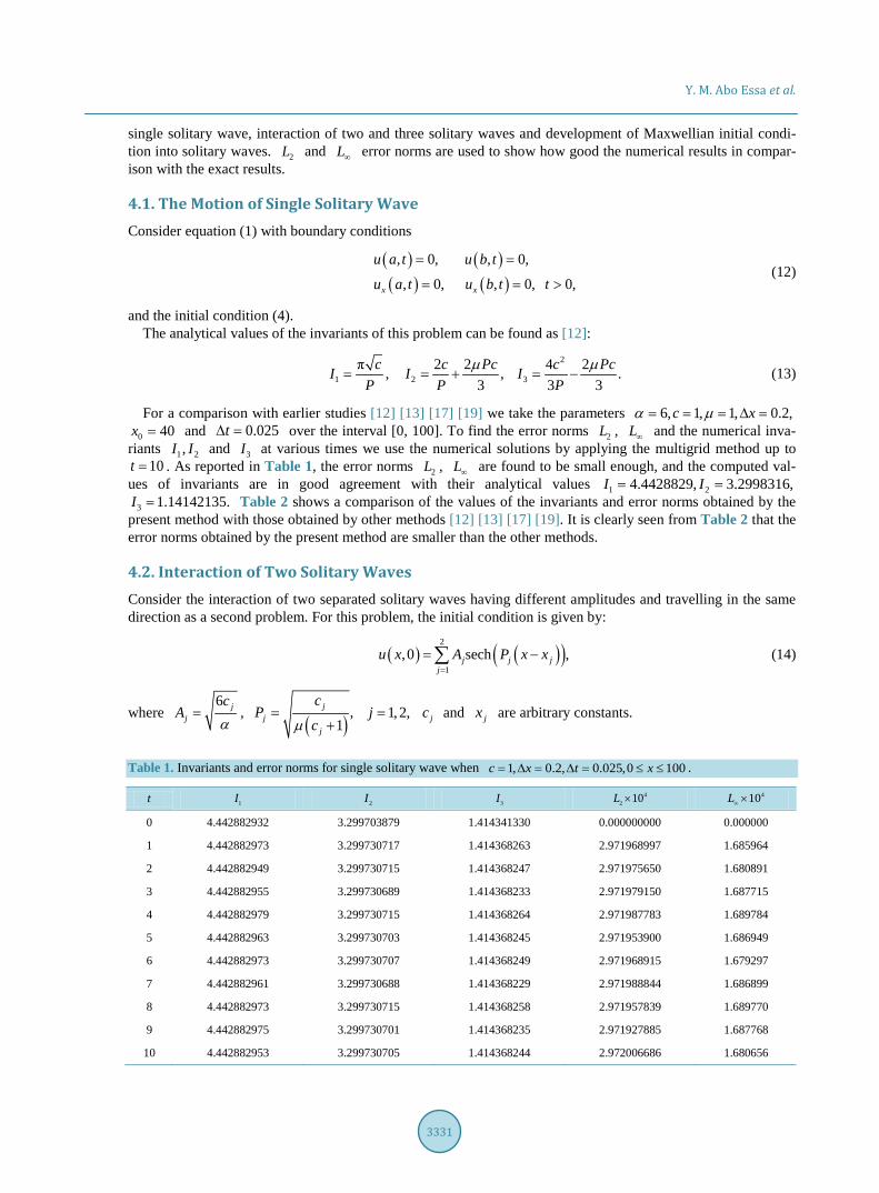
For a comparison with earlier studies [12] [13] [17] [19] we take the parameters 6, 1, 1, 0.2,c xα µ= = = ∆ = 0 40x = and 0.025t∆ = over the interval [0, 100]. To find the error norms 2L , L∞ and the numerical inva-

riants 1 2,I I and 3I at various times we use the numerical solutions by applying the multigrid method up to 10t = . As reported in Table 1, the error norms 2L , L∞ are found to be small enough, and the computed val-

ues of invariants are in good agreement with their analytical values 1 24.4428829, 3.2998316,I I= =3 1.14142135.I = Table 2 shows a comparison of the values of the invariants and error norms obtained by the

present method with those obtained by other methods [12] [13] [17] [19]. It is clearly seen from Table 2 that the error norms obtained by the present method are smaller than the other methods.

4.2. Interaction of Two Solitary Waves Consider the interaction of two separated solitary waves having different amplitudes and travelling in the same direction as a second problem. For this problem, the initial condition is given by:

( ) ( )( )2

1,0 sech ,j j j

ju x A P x x

=

= −∑ (14)

where 6 j

j

cA

α= ,

( ),

1j

jj

cP

cµ=

+ 1, 2,j = jc and jx are arbitrary constants.

Table 1. Invariants and error norms for single solitary wave when 1, 0.2, 0.025,0 100c x t x= ∆ = ∆ = ≤ ≤ .

t 1I 2I 3I 42 10L × 410L∞ ×

0 4.442882932 3.299703879 1.414341330 0.000000000 0.000000

1 4.442882973 3.299730717 1.414368263 2.971968997 1.685964

2 4.442882949 3.299730715 1.414368247 2.971975650 1.680891

3 4.442882955 3.299730689 1.414368233 2.971979150 1.687715

4 4.442882979 3.299730715 1.414368264 2.971987783 1.689784

5 4.442882963 3.299730703 1.414368245 2.971953900 1.686949

6 4.442882973 3.299730707 1.414368249 2.971968915 1.679297

7 4.442882961 3.299730688 1.414368229 2.971988844 1.686899

8 4.442882973 3.299730715 1.414368258 2.971957839 1.689770

9 4.442882975 3.299730701 1.414368235 2.971927885 1.687768

10 4.442882953 3.299730705 1.414368244 2.972006686 1.680656

Y. M. Abo Essa et al.

3332

Table 2. Comparison of errors and invariants for single solitary wave when 1, 0.2, 0.025,0 100c x t x= ∆ = ∆ = ≤ ≤ at 10.t = .

Method 1I 2I 3I 3

2 10L × 310L∞ ×

Analytical 4.4428829 3.2998316 1.4142135 0 0

Present 4.4428829 3.2997307 1.4143682 0.297201 0.1680656

[19] 4.4431758 3.3003023 1.4146927 2.41552 1.07974

Cubic B-splines coll-CN [12] 4.442 3.299 1.413 16.39 9.24

Cubic B-splines coll+PA-CN [12] 4.440 3.296 1.411 20.3 11.2

Cubic B-splines coll [13] 4.44288 3.29983 1.41420 9.30196 5.43718

MQ [17] 4.4428829 3.29978 1.414163 3.914 2.019

IMQ [17] 4.4428611 3.29978 1.414163 3.914 2.019

IQ [17] 4.4428794 3.29978 1.414163 3.914 2.019

GA [17] 4.4428829 3.29978 1.414163 3.914 2.019

TPS [17] 4.4428821 3.29972 1.414104 4.428 2.306

For the computational discussion, we use parameters 1 26, 1, 0.03, 0.01,c cα µ= = = = 1 18x = and 2 58x =

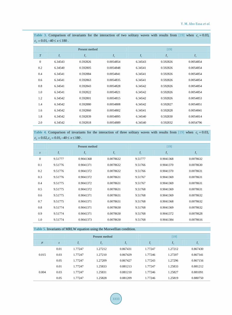
over the rang [ ]40,180− to coincide with those used by [19]. The experiment is run from 0t = to 2t = and values of the invariant quantities 1 2,I I and 3I are listed in Table 3.

Table 3 shows a comparison of the values of the invariants obtained by present method with those obtained in [19]. It is seen that the numerical values of the invariants remain almost constant during the computer run.

4.3. Interaction of Three Solitary Waves In this section, the behavior of the interaction of three solitary waves having different amplitudes and travelling in the same direction was studied. So, we consider Equation (1) with the initial condition given by the linear sum of three well-separated solitary waves of different amplitudes:

( ) ( )( )3

1,0 sech ,j j j

ju x A P x x

=

= −∑ (15)

where 6 j

j

cA

α= ,

( ),

1j

jj

cP

cµ=

+ 1, 2,3,j = jc and jx are arbitrary constants.

For the computational work, we used parameters 1 2 36, 1, 0.03, 0.02, 0.01,c c cα µ= = = = = 1 28, 48x x= = and 3 88x = over the rang [ ]40,180− . The experiment is run up to time 1t = and numerical values of the in-variant quantities 1 2,I I and 3I are displayed in Table 4.

Table 4 shows a comparison of the values of the invariants obtained by the present method with those ob-tained in [19]. It is seen that the numerical values of the invariants remain almost constant during the computer run.

4.4. The Maxwellian Initial Condition Finally, the development of the Maxwellian initial condition:

( ) ( )( )2,0 exp 40 ,u x x= − − (16)

into a train of solitary waves is discussed. It is known that the behavior of the solution with the Maxwellian con-dition (16) depends on the values of µ . So, we study each of two cases: 0.015µ = and 0.004.µ =

Table 5 contains the obtained numerical values of the invariants and a comparison of the values of the inva-riants obtained by present method with those obtained in [19].

Y. M. Abo Essa et al.

3333

Table 3. Comparison of invariants for the interaction of two solitary waves with results from [19] when 1 0.03,c =

2 0.01, 40 180c x= − ≤ ≤ .

Present method [19]

T 1I 2I 3I 1I 2I 3I

0 6.34543 0.592826 0.0054854 6.34543 0.592826 0.0054854

0.2 6.34540 0.592805 0.0054848 6.34541 0.592826 0.0054854

0.4 6.34541 0.592884 0.0054841 6.34541 0.592826 0.0054854

0.6 6.34541 0.592863 0.0054835 6.34541 0.592826 0.0054854

0.8 6.34541 0.592843 0.0054828 6.34542 0.592826 0.0054854

1.0 6.34541 0.592822 0.0054821 6.34542 0.592826 0.0054854

1.2 6.34542 0.592801 0.0054815 6.34542 0.592826 0.0054853

1.4 6.34542 0.592880 0.0054808 6.34542 0.592827 0.0054851

1.6 6.34542 0.592860 0.0054802 6.34541 0.592828 0.0054841

1.8 6.34542 0.592839 0.0054895 6.34540 0.592830 0.0054814

2.0 6.34542 0.592818 0.0054889 6.34540 0.592832 0.0054796

Table 4. Comparison of invariants for the interaction of three solitary waves with results from [19] when 1 0.03,c =

2 30.02, 0.01, 40 180c c x= = − ≤ ≤ .

Present method [19]

t 1I 2I 3I 1I 2I 3I

0 9.51777 0.9041368 0.0078632 9.51777 0.9041368 0.0078632

0.1 9.51776 0.9041371 0.0078632 9.51766 0.9041370 0.0078630

0.2 9.51776 0.9041372 0.0078632 9.51766 0.9041370 0.0078631

0.3 9.51776 0.9041372 0.0078631 9.51767 0.9041369 0.0078631

0.4 9.51775 0.9041372 0.0078631 9.51767 0.9041369 0.0078631

0.5 9.51775 0.9041372 0.0078631 9.51768 0.9041369 0.0078631

0.6 9.51775 0.9041371 0.0078631 9.51768 0.9041369 0.0078632

0.7 9.51775 0.9041371 0.0078631 9.51768 0.9041368 0.0078632

0.8 9.51774 0.9041371 0.0078630 9.51768 0.9041369 0.0078632

0.9 9.51774 0.9041371 0.0078630 9.51768 0.9041372 0.0078628

1.0 9.51774 0.9041373 0.0078630 9.51768 0.9041384 0.0078616

Table 5. Invariants of MRLW equation using the Maxwellian condition.

Present method [19]

µ t 1I 2I 3I 1I 2I 3I

0.015

0.01 1.77247 1.27212 0.867431 1.77247 1.27212 0.867430

0.03 1.77247 1.27210 0.867429 1.77246 1.27207 0.867341

0.05 1.77247 1.27209 0.867427 1.77243 1.27296 0.867156

0.004

0.01 1.77247 1.25833 0.881213 1.77247 1.25833 0.881212

0.03 1.77247 1.25831 0.881210 1.77246 1.25827 0.881091

0.05 1.77247 1.25828 0.881209 1.77246 1.25819 0.880750

Y. M. Abo Essa et al.

3334

5. Conclusion In this work we extended the use of multigrid technique to initial boundary value problems, namely the MRLW problem. We tested our scheme through single solitary wave in which the analytic solution is known. Our scheme was extended to study the interaction of two and three solitary waves and Maxwellian initial condition where the analytic solutions are unknown during the interaction. The performance and accuracy of the method were shown by calculating the error norms 2L , L∞ and conservative properties of mass, momentum and energy. The computed results showed that the present scheme is a successful numerical technique for solving the MRLW problem.

References [1] Brandt, A. (1977) Multi-Level Adaptive Solution to Boundary-Value Problem. Mathematics of Computation, 31, 333-

390. http://dx.doi.org/10.1090/S0025-5718-1977-0431719-X [2] Goldstein, C.I. (1989) Analysis and Application of Multigrid Preconditioners for Singularly Perturbed Boundary Value

Problems. SIAM Journal on Numerical Analysis, 26, 1090-1123. http://dx.doi.org/10.1137/0726061 [3] Dennis, J.C. (1984) Multigrid Method for Partial Differential Equations. Studies in numerical Analysis, 24. [4] Hachbusch, W. (1984) Multigrid Methods and Applications. Springer, Berlin. [5] Brandt, A. (1988) Multilevel Computations. Marcel Dekker, New York. [6] Wesseling, P. (1992) An Introduction to Multigrid Methods. John Wiley & Sons, New York. [7] Hassen, N.A., Osama, E.M. and Fatema, H.M. (1995) The Relaxation Schemes for the Two Dimensional Anisotropic

Partial Differential Equations Using Multigrid Method. 20th INI Conf. for Stat., Comp. Sci., Scient. & Social Appl., 3-9 April 1995, Cairo.

[8] Abo Essa, Y.M., Amer, T.S. and Ibrahim, I.A. (2011) Numerical Treatment of the Generalized Regularized Long- Wave Equation. Far East Journal of Applied Mathematics, 52, 147-154.

[9] Abo Essa, Y.M., Amer, T.S. and Abdul-Moniem, I.B. (2012) Application of Multigrid Technique for the Numerical Solution of the Non-Linear Dispersive Waves Equations. International Journal of Mathematical Archive, 3, 4903- 4910.

[10] Peregrine, D.H. (1966) Calculations of the Development of an Undular Bore. Journal of Fluid Mechanics, 25, 321-330. http://dx.doi.org/10.1017/S0022112066001678

[11] Benjamin, T.B., Bona, J.L. and Mahony, J.L. (1972) Model Equations for Long Waves in Nonlinear Dispersive Sys-tems. Philosophical Transactions of the Royal Society of London. Series A, 272, 47-78. http://dx.doi.org/10.1098/rsta.1972.0032

[12] Gardner, L.R.T., Gardner, G.A., Ayub, F.A. and Amein, N.K. (1997) Approximations of Solitary Waves of the MRLW Equation by B-Spline Finite Element. Arabian Journal for Science and Engineering, 22, 183-193.

[13] Khalifa, A.K., Raslan, K.R. and Alzubaidi, H.M. (2008) A Collocation Method with Cubic B-Splines for Solving the MRLW Equation. Journal of Computational and Applied Mathematics, 212, 406-418. http://dx.doi.org/10.1016/j.cam.2006.12.029

[14] Khalifa, A.K., Raslan, K.R. and Alzubaidi, H.M. (2007) A Finite Difference Scheme for the MRLW and Solitary Wave Interactions. Applied Mathematics and Computation, 189, 346-354. http://dx.doi.org/10.1016/j.amc.2006.11.104

[15] Raslan, K.R. (2009) Numerical Study of the Modified Regularized Long Wave (MRLW) Equation. Chaos, Solitons and Fractals, 42, 1845-1853. http://dx.doi.org/10.1016/j.chaos.2009.03.098

[16] Raslan, K.R. and Hassan, S.M. (2009) Solitary Waves of the MRLW Equation. Applied Mathematics Letters, 22, 984- 989. http://dx.doi.org/10.1016/j.aml.2009.01.020

[17] Ali, A. (2009) Mesh Free Collocation Method for Numerical Solution of Initial-Boundary Value Problems Using Ra-dial Basis Functions. Ph.D. Thesis, Ghulam Ishaq Khan Institute of Engineering Sciences and Technology, Khyber Pakhtunkhwa.

[18] Haq, F., Islam, S. and Tirmizi, I.A. (2010) A Numerical Technique for Solution of the MRLW Equation Using Quartic B-Splines. Applied Mathematical Modelling, 34, 4151-4160. http://dx.doi.org/10.1016/j.apm.2010.04.012

[19] Battal Gazi Karakoc, S. and Geyikli, T. (2013) Petrov-Galerkin Finite Element Method for Solving the MRLW Equa-tion. Mathematical Sciences, 7, 25.