the mythical swing voter - columbia universitygelman/research/published/swingers.pdf · the...

Quarterly Journal of Political Science, 2016, 11: 103–130

The Mythical Swing Voter

Andrew Gelman1, Sharad Goel2, Douglas Rivers3 andDavid Rothschild4∗

1Columbia University, USA; [email protected] University, USA; [email protected] University, USA; [email protected] Research, USA; [email protected]

ABSTRACT

Most surveys conducted during the 2012 U.S. presidentialcampaign showed large swings in support for the Demo-cratic and Republican candidates, especially before andafter the first presidential debate. Using a combination oftraditional cross-sectional surveys, a unique panel survey (interms of scale, frequency, and source), and a high responserate panel, we find that daily sample composition variedmore in response to campaign events than did vote inten-tions. Multilevel regression and post-stratification (MRP)is used to correct for this selection bias. Demographic post-stratification, similar to that used in most academic andmedia polls, is inadequate, but the addition of attitudinalvariables (party identification, ideological self-placement,and past vote) appears to make selection ignorable in ourdata. We conclude that vote swings in 2012 were mostlysample artifacts and that real swings were quite small. Whilethis account is at odds with most contemporaneous analyses,

∗We thank Jake Hofman, Neil Malhotra, and Duncan Watts for their comments,and the National Science Foundation for partial support for this research. Wealso thank the audiences at MPSA, AAPOR, Toulouse Network for Information

Supplementary Material available from:http://dx.doi.org/10.1561/100.00015031_suppMS submitted on 26 February 2015; final version received 30 November 2015ISSN 1554-0626; DOI 10.1561/100.00015031© 2016 A. Gelman, S. Goel, D. Rivers and D. Rothschild

104 Gelman et al.

it better corresponds with our understanding of partisanpolarization in modern American politics.

Keywords: Elections; swing voters; multilevel regression and post-stratification

1 Introduction

In a competitive political environment, a relatively small number ofvoters can shift control of Congress and the Presidency from one partyto the other, or to divided government. Polls do indeed show substantialvariation in voting intentions over the course of campaigns. This suggeststhat swing voters are key to understanding the changing fortunes ofDemocrats and Republicans in recent national elections. This is certainlythe view of political professionals and media observers. Campaignsspend enormous sums — over $2.6 billion in the 2012 presidentialelection cycle — trying to target “persuadable voters.” Poll aggregatorstrack day-to-day swings in the proportion of voters supporting eachcandidate. Political scientists have debated whether swings in thepolls are a response to campaign events or are reversions to predictablepositions as voters become more informed about the candidates (Gelmanand King, 1993; Hillygus and Jackman, 2003; Kaplan et al., 2012).Both researchers and campaign participants seem to agree that pollsaccurately measure vote intentions and that these are malleable. Whilethere is disagreement about the causes of swings, no one appears tohave questioned their existence.

But there is a puzzle: candidates appeal to swing voters in debates,campaigns target advertising toward swing voters, journalists discussswing voters, and the polls do indeed swing — but it is hard to findvoters who have actually switched sides. Partly this is because mostpolls are based on independent cross-sections of respondents, and sovote switching cannot be directly observed.1 But there are also theo-retical reasons to be skeptical about the degree of volatility found in

Technology, Stanford, Microsoft Research, University of Pennsylvania, Duke, andSanta Clara for their feedback during talks on this work.

1Individual-level changes must be inferred from aggregate shifts in candidatepreference between polls, and this inference depends upon the assumption that the

The Mythical Swing Voter 105

election polls. If, as is widely agreed, there is a high degree of partisanpolarization in the American electorate, it seems implausible that manyvoters will switch support from one party to the other because of minorcampaign events (Baldassarri and Gelman, 2008; Fiorina and Abrams,2008; Levendusky, 2009).2

In this paper we focus on apparent vote shifts surrounding thedebates between Barack Obama and Mitt Romney during the 2012U.S. presidential election campaign. We argue that the apparent swingsin vote intention represent mostly changes in sample composition —not changes in opinion — and that these “phantom swings” arise fromsample selection bias in survey participation. To make this case, wedraw on three sources of evidence: (1) traditional cross-sectional surveys;(2) a novel large-scale panel survey; and (3) the RAND American LifePanel. Previous studies have tended to assume that campaign eventscause changes in vote intentions, while ignoring the possibility thatthey may cause changes in survey participation. We show that in 2012,campaign events were more strongly correlated with changes in surveyparticipation than with changes in vote intention. As a consequence,inferences about the impact of campaign events from changes in pollingaverages involve invalid sample comparisons, similar to uncontrolleddifferences among treatment groups.

We further show how one can correct for this sample bias. If surveyvariables such as vote intention are independent of sample selectionconditional upon a set of covariates, various methods can be used toobtain consistent estimates of population parameters. Using the methodof multilevel regression and post-stratification (MRP), we show thatconditioning upon standard demographics (age, race, gender, education)is inadequate to remove the selection bias present in our data. However,the introduction of controls for party ID, ideology, and past vote amongthe covariates appears to substantially eliminate selection effects. While

sample selection mechanism does not change at the same time. Of course, voteswitching is directly observable in panel data, but there are few election panels withmultiple interviews of the same respondents, and even fewer panels are large enoughto provide reliable estimates of even moderate-sized vote swings.

2To be clear, we are discussing net change in support for candidates. Panelsurveys show much larger amounts of gross change in vote intention between waveswhich are offset by changes in the opposite direction. See, for example, Table 7.1 ofSides and Vavreck (2014).

106 Gelman et al.

the use of party ID weighting is controversial in cross-sectional studies(Allsop and Weisberg, 1988; Kaminska and Barnes, 2008), most of theseproblems can be avoided in a panel design.3 In panels, post-stratificationon baseline attitudes avoids endogeneity problems associated with cross-sectional party ID weighting, even if these attitudes are not stable overthe campaign.

2 Evidence from Empirical Studies

2.1 Study 1: Sample Selection Bias in Cross-sectional Polls

In mid-September, Obama led Romney by about 4% in the HuffingtonPost polling average and seemed to be coasting to an easy reelectionvictory. However, as shown in Figure 1a, following the first presidentialdebate on October 3, the polls reversed and Romney led in nine of thetwelve polls conducted in the following week (of the remaining three,one was a tie and Obama led in the other two). On average, Romneyled Obama by slightly over 1% in the polls with field periods startingbetween October 4 and 8. It was not until after the third debate (onOctober 22) that Obama regained a small lead in the polling averages,which he maintained until election day. At the time, it was commonlyagreed that Obama had performed poorly in the first presidential debatebut had recovered in later debates. This account is consistent with theexistence of a pool of swing voters who switched back and forth betweenthe candidates.

However, other data from the same surveys cast doubt on the claimthat the first presidential debate caused a swing of this magnitude.Consider, for example, the Pew Research surveys. In the September12–16 Pew survey, Obama led Romney 51–42 among registered voters,but the two candidates were tied 46–46 in the October 4–7 survey. The5% swing to Romney sounds impressive until it is compared to howthe same respondents recalled voting in 2008. In the September 12–16sample, 47% recalled voting for Obama in 2008, but this dropped to42% in the October 4–7 sample. Recalled vote for McCain also rose

3See Reilly et al. (2001) for a potential work-around in cross-sectional studies.


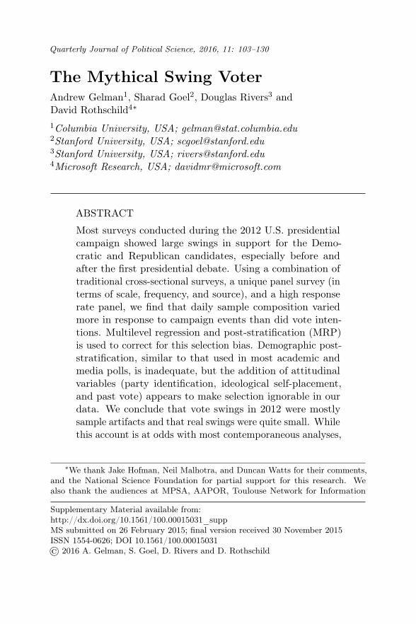
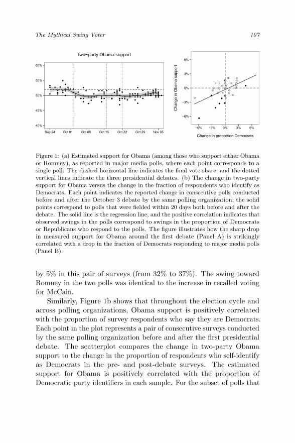
Figure 1: (a) Estimated support for Obama (among those who support either Obamaor Romney), as reported in major media polls, where each point corresponds to asingle poll. The dashed horizontal line indicates the final vote share, and the dottedvertical lines indicate the three presidential debates. (b) The change in two-partysupport for Obama versus the change in the fraction of respondents who identify asDemocrats. Each point indicates the reported change in consecutive polls conductedbefore and after the October 3 debate by the same polling organization; the solidpoints correspond to polls that were fielded within 20 days both before and after thedebate. The solid line is the regression line, and the positive correlation indicates thatobserved swings in the polls correspond to swings in the proportion of Democratsor Republicans who respond to the polls. The figure illustrates how the sharp dropin measured support for Obama around the first debate (Panel A) is strikinglycorrelated with a drop in the fraction of Democrats responding to major media polls(Panel B).

by 5% in this pair of surveys (from 32% to 37%). The swing towardRomney in the two polls was identical to the increase in recalled votingfor McCain.

Similarly, Figure 1b shows that throughout the election cycle andacross polling organizations, Obama support is positively correlatedwith the proportion of survey respondents who say they are Democrats.Each point in the plot represents a pair of consecutive surveys conductedby the same polling organization before and after the first presidentialdebate. The scatterplot compares the change in two-party Obamasupport to the change in the proportion of respondents who self-identifyas Democrats in the pre- and post-debate surveys. The estimatedsupport for Obama is positively correlated with the proportion ofDemocratic party identifiers in each sample. For the subset of polls that

108 Gelman et al.

were in the field within 20 days before and after the debate (indicatedby the solid points), the effect is even more pronounced.

There are at least two potential explanations for these patterns inthe data. One possibility is that the debate changed people’s votingintentions, their memory of how they had voted in the previous election,and their party identification (Himmelweit et al., 1978). Or, alterna-tively, the samples before and after the first debate were different (i.e.,the pre-debate surveys contained more Democrats and 2008 Obamavoters, while the ones afterward contained more Republicans and 2008McCain voters).

It is impossible to distinguish between these explanations usingcross-sectional data. Respondents in the September and October Pewsamples do not overlap, so we cannot tell whether more of the Septemberrespondents would have supported Romney if they had been reinter-viewed in October. The October interviews are with a different sampleand, while more say they intend to vote for Romney than those in theSeptember sample, we do not know whether these respondents were lesssupportive of Romney in September, since they were not interviewed inSeptember.

2.2 Study 2: The Xbox Panel Survey

2.2.1 Survey Design and Methodology

We address the shortcomings of cross-sectional surveys discussed aboveby fielding a large-scale online panel survey. During the 2012 U.S.presidential campaign, we conducted 750,148 interviews with 345,858unique respondents on the Xbox gaming platform during the 45 dayspreceding the election. Xbox Live subscribers were asked to providebaseline information about themselves in a registration survey, includingdemographics, party identification, and ideological self-placement. Eachday, a new survey was offered and respondents could choose whetherthey wished to complete it. The analysis reported here is based upon the83,283 users who responded at least once prior to the first presidentialdebate on October 3. In total, these respondents completed 336,805interviews, or an average of about four interviews per respondent. Over20,000 panelists completed at least five interviews and over 5,000 an-swered surveys on 15 or more days. The average number of respondentsin our analysis sample each day was about 7,500. The Xbox panel


provides abundant data on actual shifts in vote intention by a particularset of voters during the 2012 presidential campaign, and the size ofthe Xbox panel supports estimation of MRP models which adjust fordifferent types of selection bias.

Our analysis has two steps. We first show that with demographicadjustments, the Xbox data reproduce swings found in media pollsduring the 2012 campaign. That is, if one adjusts for the variables typi-cally used for weighting phone or Internet samples, daily Xbox surveysexhibit the same sort of patterns found in conventional polls. Second,because the Xbox data come from a panel with baseline measurementsof party ID and other attitudes, it is feasible to correct for variations insurvey participation due to partisanship, ideology, and past vote. Thecorrelation of within-panel response rates with party ID, for example,varies over the course of the campaign. Using MRP with an expandedset of covariates enables us to distinguish between actual vote swingsand compositional changes in daily samples. With these adjustments,most of the apparent swings in vote intention disappear.

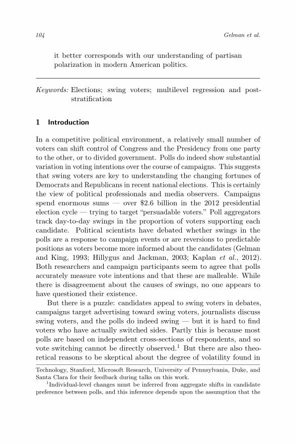
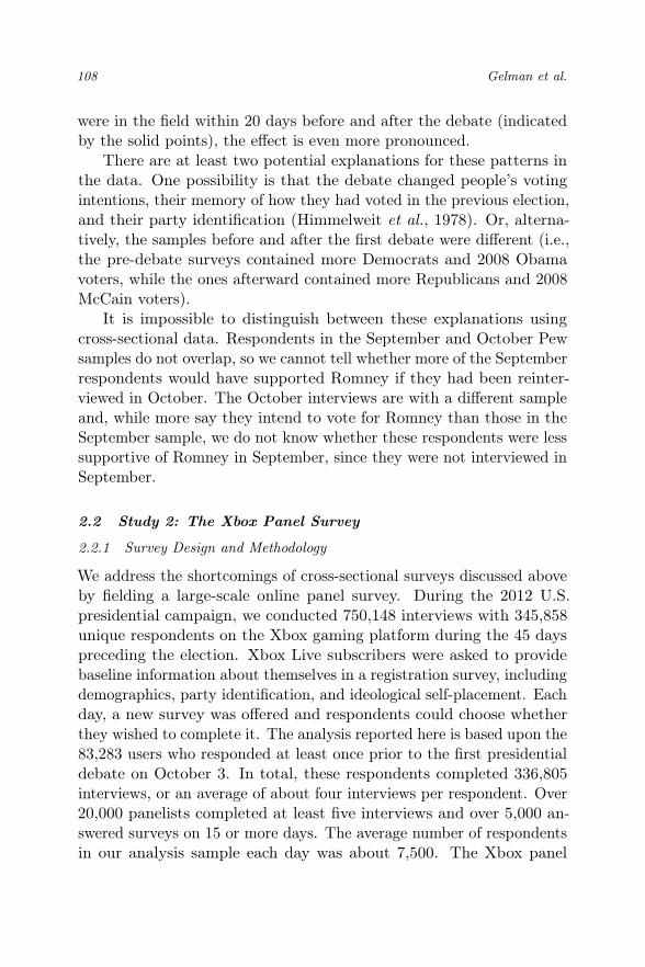
The Xbox panel is not representative of the electorate, with Xboxrespondents predominantly young and male. As shown in Figure 2,

Figure 2: Demographic and partisan composition of the Xbox panel and the 2008electorate. There are large differences in the age distribution and gender compositionof the Xbox panel and the 2012 exit poll. Without adjustment, Xbox data consistentlyoverstate support for Romney. However, the large size of the Xbox panel permitssatisfactory adjustment even for large skews.

110 Gelman et al.

66% of Xbox panelists are between 18 and 29 years old, compared toonly 18% of respondents in the 2008 exit poll,4 while men make up93% of Xbox panelists but only 47% of voters in the exit poll. With atypical-sized sample of 1,000 or so, it would be difficult to correct skewsthis large, but the scale of the Xbox panel compensates for its manysins. For example, despite the small proportion of women among Xboxpanelists, there are over 5,000 women in our sample, which is an orderof magnitude more than the number of women in an RDD sample of1,000.

The method of MRP is described in Gelman and Little (1997).Briefly, post-stratification is a standard framework for correcting forknown differences between sample and target populations (Little, 1993).The idea is to partition the population into cells (defined by the cross-classification of various attributes of respondents), use the sample toestimate the mean of a survey variable within each cell, and finally toaggregate the cell-level estimates by weighting each cell by its proportionin the population. In conventional post-stratification, cell means areestimated using the sample mean within each cell. This estimate isunbiased if selection is ignorable (i.e., if sample selection is independentof survey variables conditional upon the variables defining the post-stratification). In other words, the key assumption is that within eachcell individuals who partake in the survey have vote choices suitablysimilar to those who choose not to take the survey to make them feasiblesubstitutes for the non-responders. This ignorability assumption is moreplausible if more variables are conditioned upon. However, adding morevariables to the post-stratification increases the number of cells at anexponential rate. If any cell is empty in the sample (which is guaranteedto occur if the number of cells exceeds the sample size), then theconventional post-stratification estimator is not defined. Even if everycell is nonempty, there can still be problems because estimates of cellmeans are noisy in small cells. Collapsing cells reduces variability,but can leave substantial amounts of selection bias. MRP addressesthis problem by using hierarchical Bayesian regression to obtain stable

4As discussed later, we chose to use the 2008 exit poll data for post-stratificationso that the analysis relies only upon information available before the 2012 election.Relying upon 2008 data demonstrates the feasibility of this approach for forecasting.Similar results are obtained by post-stratifying on 2012 exit poll demographics andattitudes.


estimates of cell means (Gelman and Hill, 2006). This technique hasbeen successfully used in the study of public opinion and voting (Ghitzaand Gelman, 2013; Lax and Phillips, 2009).

We initially apply MRP by partitioning the population into 6,258cells based upon demographics and state of residence (2 gender ⇥ 4 race⇥ 4 age ⇥ 4 education ⇥ 50 states plus the District of Columbia).5 Onecell, for example, corresponds to 30- to 44-year-old white male collegegraduates living in California. Using each day’s sample, we then fitseparate multilevel logistic regression models that predict respondents’stated vote intention on that day as a function of their demographicattributes. Key to our analysis is that cells means (i.e., average voteintention) on any given day are accurately estimated by the regressionmodels. We evaluate this assumption in the Appendix and find themodel indeed generates accurate group-level estimates despite beingbased on a non-representative sample of respondents. We additionallyassume that the distribution of voter demographics for each state wouldbe the same as that found in the 2008 exit poll. See the Appendix foradditional details on modeling and methods.

2.2.2 Xbox Panel Results

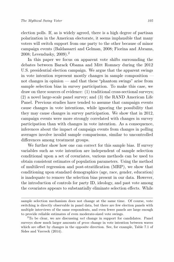
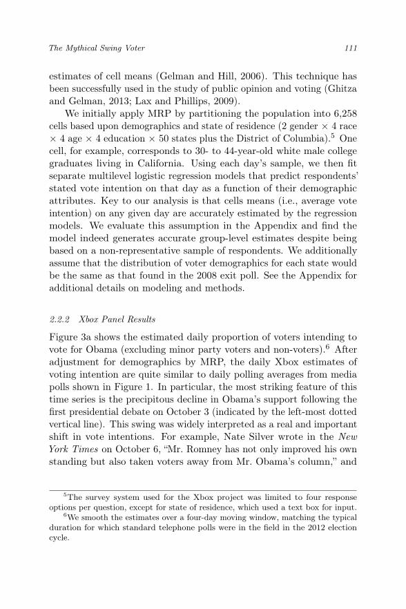
Figure 3a shows the estimated daily proportion of voters intending tovote for Obama (excluding minor party voters and non-voters).6 Afteradjustment for demographics by MRP, the daily Xbox estimates ofvoting intention are quite similar to daily polling averages from mediapolls shown in Figure 1. In particular, the most striking feature of thistime series is the precipitous decline in Obama’s support following thefirst presidential debate on October 3 (indicated by the left-most dottedvertical line). This swing was widely interpreted as a real and importantshift in vote intentions. For example, Nate Silver wrote in the NewYork Times on October 6, “Mr. Romney has not only improved his ownstanding but also taken voters away from Mr. Obama’s column,” and

5The survey system used for the Xbox project was limited to four responseoptions per question, except for state of residence, which used a text box for input.

6We smooth the estimates over a four-day moving window, matching the typicalduration for which standard telephone polls were in the field in the 2012 electioncycle.

112 Gelman et al.

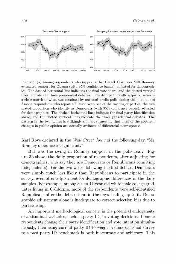
Figure 3: (a) Among respondents who support either Barack Obama or Mitt Romney,estimated support for Obama (with 95% confidence bands), adjusted for demograph-ics. The dashed horizontal line indicates the final vote share, and the dotted verticallines indicate the three presidential debates. This demographically adjusted series isa close match to what was obtained by national media polls during this period. (b)Among respondents who report affiliation with one of the two major parties, the esti-mated proportion who identify as Democrats (with 95% confidence bands), adjustedfor demographics. The dashed horizontal lines indicate the final party identificationshare, and the dotted vertical lines indicate the three presidential debates. Thepattern in the two figures is strikingly similar, suggesting that most of the apparentchanges in public opinion are actually artifacts of differential nonresponse.

Karl Rove declared in the Wall Street Journal the following day, “Mr.Romney’s bounce is significant.”

But was the swing in Romney support in the polls real? Fig-ure 3b shows the daily proportion of respondents, after adjusting fordemographics, who say they are Democrats or Republicans (omittingindependents). For the two weeks following the first debate, Democratswere simply much less likely than Republicans to participate in thesurvey, even after adjustment for demographic differences in the dailysamples. For example, among 30- to 44-year-old white male college grad-uates living in California, more of the respondents were self-identifiedRepublicans after the debate than in the days leading up to it. Demo-graphic adjustment alone is inadequate to correct selection bias due topartisanship.

An important methodological concern is the potential endogeneityof attitudinal variables, such as party ID, in voting decisions. If somerespondents change their party identification and vote intention simulta-neously, then using current party ID to weight a cross-sectional surveyto a past party ID benchmark is both inaccurate and arbitrary. This


problem has deterred most media polls from using party ID for weight-ing. The approach used here, however, avoids the endogeneity problembecause we are adjusting past party ID to a past party ID benchmark.That is, current vote intention is post-stratified on a pre-determinedvariable (baseline party ID) that does not change over the course of thepanel.

The other objection to post-stratification on partisanship is that,unlike demographics (where we have Census data), we lack reliablebenchmarks for its baseline distribution. This is less of a problem thanit might seem. First, the approximate distribution of party ID can beobtained from other surveys. In our analysis, we used the 2008 exit pollfor the joint distribution of all variables. Second, the swing estimatesare not particularly sensitive to which baseline is used, since swings aresimilar within the different party ID groups. The party ID benchmarkhas a larger impact on the estimated candidate lead, but even this doesnot vary a lot within the range of plausible party ID distributions. Inthe Appendix, we compare estimates based upon covariate distributionsfrom the 2008 and 2012 exit polls, and find the two lead to similarresults.

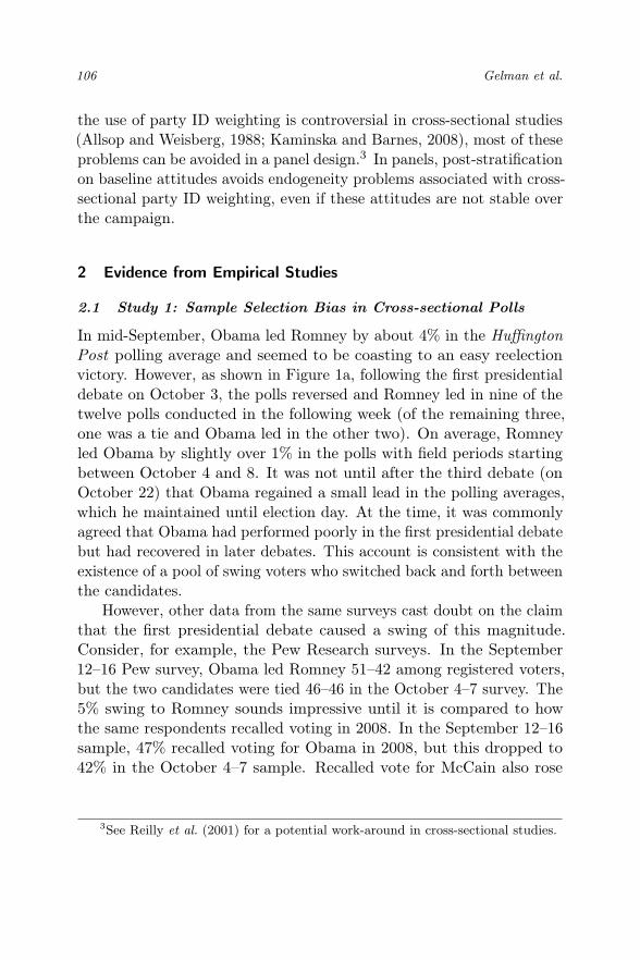
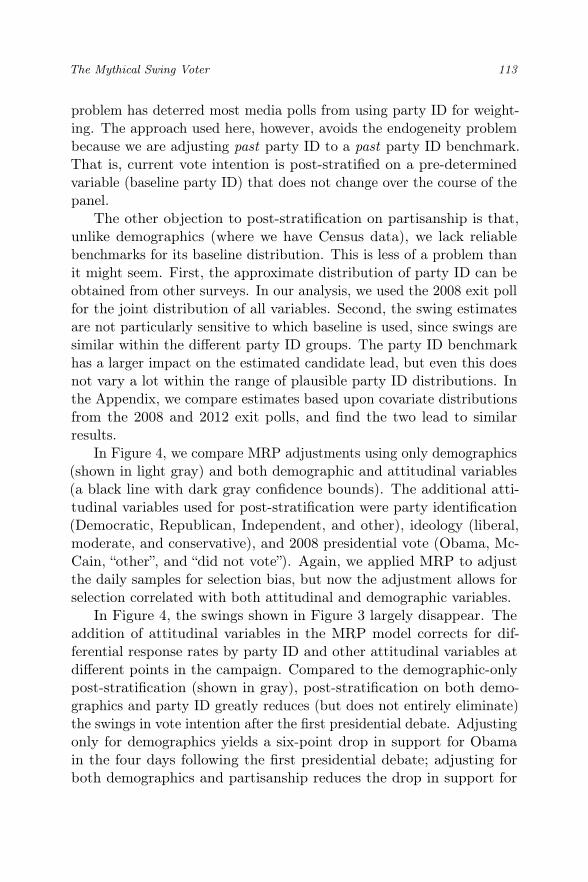
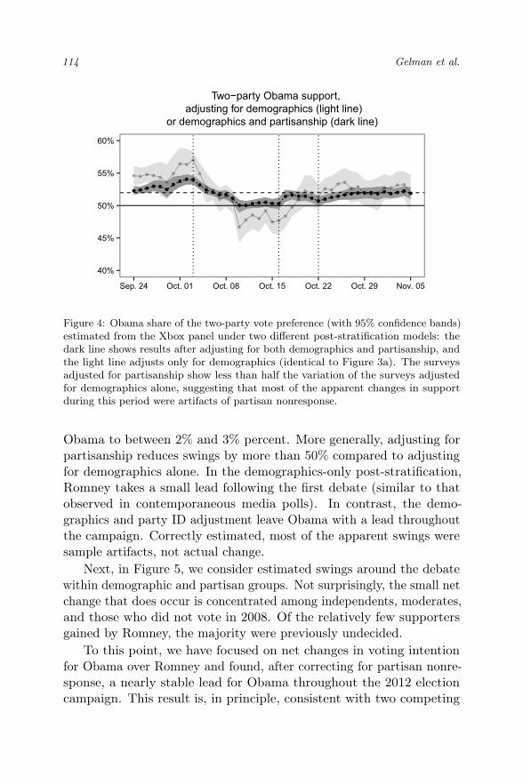
In Figure 4, we compare MRP adjustments using only demographics(shown in light gray) and both demographic and attitudinal variables(a black line with dark gray confidence bounds). The additional atti-tudinal variables used for post-stratification were party identification(Democratic, Republican, Independent, and other), ideology (liberal,moderate, and conservative), and 2008 presidential vote (Obama, Mc-Cain, “other”, and “did not vote”). Again, we applied MRP to adjustthe daily samples for selection bias, but now the adjustment allows forselection correlated with both attitudinal and demographic variables.

In Figure 4, the swings shown in Figure 3 largely disappear. Theaddition of attitudinal variables in the MRP model corrects for dif-ferential response rates by party ID and other attitudinal variables atdifferent points in the campaign. Compared to the demographic-onlypost-stratification (shown in gray), post-stratification on both demo-graphics and party ID greatly reduces (but does not entirely eliminate)the swings in vote intention after the first presidential debate. Adjustingonly for demographics yields a six-point drop in support for Obamain the four days following the first presidential debate; adjusting forboth demographics and partisanship reduces the drop in support for

114 Gelman et al.

40%

45%

50%

55%

60%

Sep. 24 Oct. 01 Oct. 08 Oct. 15 Oct. 22 Oct. 29 Nov. 05

Two−party Obama support,adjusting for demographics (light line)

or demographics and partisanship (dark line)

Figure 4: Obama share of the two-party vote preference (with 95% confidence bands)estimated from the Xbox panel under two different post-stratification models: thedark line shows results after adjusting for both demographics and partisanship, andthe light line adjusts only for demographics (identical to Figure 3a). The surveysadjusted for partisanship show less than half the variation of the surveys adjustedfor demographics alone, suggesting that most of the apparent changes in supportduring this period were artifacts of partisan nonresponse.

Obama to between 2% and 3% percent. More generally, adjusting forpartisanship reduces swings by more than 50% compared to adjustingfor demographics alone. In the demographics-only post-stratification,Romney takes a small lead following the first debate (similar to thatobserved in contemporaneous media polls). In contrast, the demo-graphics and party ID adjustment leave Obama with a lead throughoutthe campaign. Correctly estimated, most of the apparent swings weresample artifacts, not actual change.

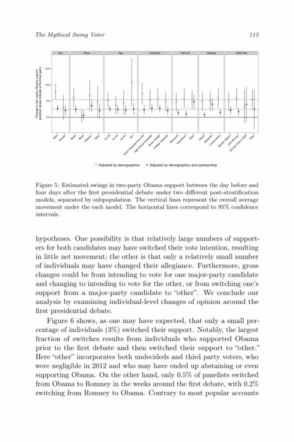
Next, in Figure 5, we consider estimated swings around the debatewithin demographic and partisan groups. Not surprisingly, the small netchange that does occur is concentrated among independents, moderates,and those who did not vote in 2008. Of the relatively few supportersgained by Romney, the majority were previously undecided.

To this point, we have focused on net changes in voting intentionfor Obama over Romney and found, after correcting for partisan nonre-sponse, a nearly stable lead for Obama throughout the 2012 electioncampaign. This result is, in principle, consistent with two competing


Figure 5: Estimated swings in two-party Obama support between the day before andfour days after the first presidential debate under two different post-stratificationmodels, separated by subpopulation. The vertical lines represent the overall averagemovement under the each model. The horizontal lines correspond to 95% confidenceintervals.

hypotheses. One possibility is that relatively large numbers of support-ers for both candidates may have switched their vote intention, resultingin little net movement; the other is that only a relatively small numberof individuals may have changed their allegiance. Furthermore, grosschanges could be from intending to vote for one major-party candidateand changing to intending to vote for the other, or from switching one’ssupport from a major-party candidate to “other”. We conclude ouranalysis by examining individual-level changes of opinion around thefirst presidential debate.

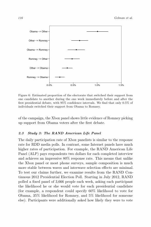
Figure 6 shows, as one may have expected, that only a small per-centage of individuals (3%) switched their support. Notably, the largestfraction of switches results from individuals who supported Obamaprior to the first debate and then switched their support to “other.”Here “other” incorporates both undecideds and third party voters, whowere negligible in 2012 and who may have ended up abstaining or evensupporting Obama. On the other hand, only 0.5% of panelists switchedfrom Obama to Romney in the weeks around the first debate, with 0.2%switching from Romney to Obama. Contrary to most popular accounts

116 Gelman et al.

Figure 6: Estimated proportion of the electorate that switched their support fromone candidate to another during the one week immediately before and after thefirst presidential debate, with 95% confidence intervals. We find that only 0.5% ofindividuals switched their support from Obama to Romney.

of the campaign, the Xbox panel shows little evidence of Romney pickingup support from Obama voters after the first debate.

2.3 Study 3: The RAND American Life Panel

The daily participation rate of Xbox panelists is similar to the responserate for RDD media polls. In contrast, some Internet panels have muchhigher rates of participation. For example, the RAND American LifePanel (ALP) pays respondents two dollars for each completed interviewand achieves an impressive 80% response rate. This means that unlikethe Xbox panel or most phone surveys, sample composition is muchmore stable between waves and interwave selection effects are minimal.To test our claims further, we examine results from the RAND Con-tinuous 2012 Presidential Election Poll. Starting in July 2012, RANDpolled a fixed panel of 3,666 people each week, asking each participantthe likelihood he or she would vote for each presidential candidate(for example, a respondent could specify 60% likelihood to vote forObama, 35% likelihood for Romney, and 5% likelihood for someoneelse). Participants were additionally asked how likely they were to vote


40%

45%

50%

55%

60%

Sep 17 Sep 24 Oct 01 Oct 08 Oct 15 Oct 22 Oct 29 Nov 05

Two−party Obama support

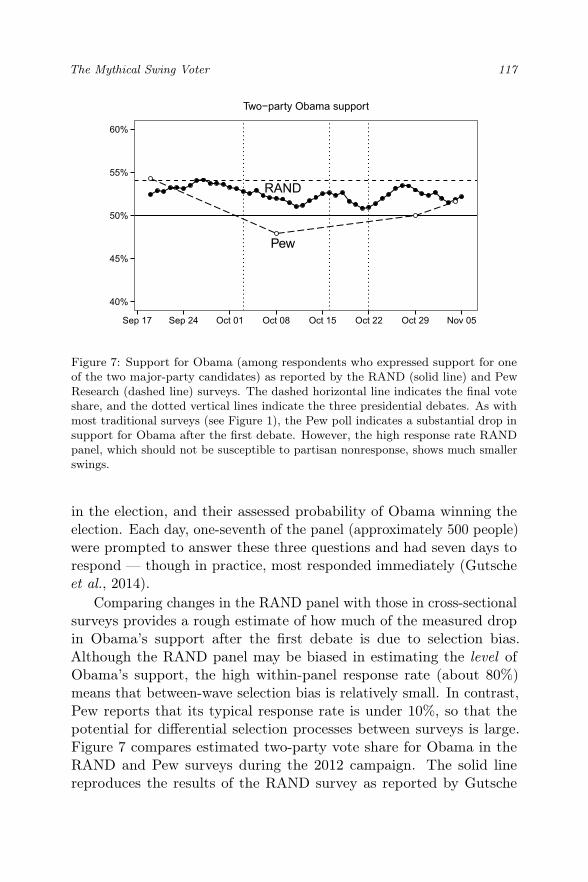
Figure 7: Support for Obama (among respondents who expressed support for oneof the two major-party candidates) as reported by the RAND (solid line) and PewResearch (dashed line) surveys. The dashed horizontal line indicates the final voteshare, and the dotted vertical lines indicate the three presidential debates. As withmost traditional surveys (see Figure 1), the Pew poll indicates a substantial drop insupport for Obama after the first debate. However, the high response rate RANDpanel, which should not be susceptible to partisan nonresponse, shows much smallerswings.

in the election, and their assessed probability of Obama winning theelection. Each day, one-seventh of the panel (approximately 500 people)were prompted to answer these three questions and had seven days torespond — though in practice, most responded immediately (Gutscheet al., 2014).

Comparing changes in the RAND panel with those in cross-sectionalsurveys provides a rough estimate of how much of the measured dropin Obama’s support after the first debate is due to selection bias.Although the RAND panel may be biased in estimating the level ofObama’s support, the high within-panel response rate (about 80%)means that between-wave selection bias is relatively small. In contrast,Pew reports that its typical response rate is under 10%, so that thepotential for differential selection processes between surveys is large.Figure 7 compares estimated two-party vote share for Obama in theRAND and Pew surveys during the 2012 campaign. The solid linereproduces the results of the RAND survey as reported by Gutsche

118 Gelman et al.

et al. (2014), where each point represents a seven-day rolling average.7The RAND estimate shows a low of 51% in Obama support occurringin the days after the first debate. This estimate is nearly identical tothe Xbox estimate of 50%. In contrast, Pew shows Obama supportdropping from 55% to 48%.

3 Discussion

By considering three qualitatively different sources of evidence — tra-ditional cross-sectional surveys, a large-scale opt-in panel, and a highresponse rate panel — we find that much of the apparent swings invote intention can be explained by sample selection bias. In panelsurveys, even ones with low response rates, real population changes canbe inferred by post-stratifying on attitudinal variables measured at thestart of the panel. In cross-sectional survey designs, it can be difficultto correct for selection bias without assuming that attitudinal variablesdo not fluctuate over time. Though the proportion of Democrats andRepublicans in presidential election exit polls is quite stable, there is alsoevidence that party ID does fluctuate somewhat between elections. Thismakes cross-sectional party ID corrections controversial, but the failureto adjust sample composition for anything other than demographicsshould be equally controversial. Methods exist for such adjustment,making use of the assumption that the post-stratifying variable (in thiscase, party identification) evolves slowly (Reilly et al., 2001). But eventhe naive approach of post-stratifying on current partisanship worksreasonably well (see the Appendix for details).

We have not treated the problem of turnout. Likelihood of votingmay vary over the campaign and the proclivity to take a survey couldbe an indicator of likelihood to vote. Consequently, it is possiblethat cross-sectional poll estimates could be good predictors of actualvote, even if they are misleading about changes in preference. Thisargument is speculative. In fact, as seen in Figure 3b, the relative

7Whereas Gutsche et al. (2014) separately plot support for Obama and Romney,we combine these two into a single line indicating two-party Obama support; weotherwise make no adjustments to their reported numbers. The estimated numberof votes for each candidate is based on one’s stated likelihood of voting, and one’sstated likelihood of voting for each candidate conditional on voting.


dearth of Democratic sample respondents was short-lived. By the thirddebate, there were as many Democrats participating in Xbox surveys asthere had been before the first. Furthermore, this runs counter to theremarkable stability of the partisan composition of the electorate: inevery presidential election from 1984 to 2012, Democrats have comprisedbetween 37% and 39% of voters, and men have comprised between 46%and 48% of voters.

The temptation to over-interpret bumps in election polls can bedifficult to resist, so our findings provide a cautionary tale. The existenceof a pivotal set of voters attentively listening to the presidential debatesand switching sides is a much more satisfying narrative, both to pollstersand survey researchers, than a small, but persistent, set of sampleselection biases. Correcting for these biases gives us a picture of publicopinion and voting that corresponds better with our understanding ofthe intense partisan polarization in modern American politics.

A Methods and Materials

Xbox survey.The only way to answer the polling questions was via the Xbox Livegaming platform. There was no invitation or permanent link to thepoll, and so respondents had to locate it daily on the Xbox Live’s homepage and click into it. The first time a respondent opted-into the poll,they were directed to answer the nine demographics questions listedbelow. On all subsequent times, respondents were immediately directedto answer between three and five daily survey questions, one of whichwas always the vote intention question.

Intention Question: If the election were held today, who would youvote for?Barack Obama\Mitt Romney\Other\Not Sure

Demographics Questions:

1. Who did you vote for in the 2008 Presidential election?Barack Obama\John McCain\Other candidate\Did not vote in2008

120 Gelman et al.

Figure A.1: The left panel shows the vote intention question, and the right panelshows what respondents were presented with during their first visit to the poll.

2. Thinking about politics these days, how would you describe yourown political viewpoint?Liberal\Moderate\Conservative\Not sure

3. Generally speaking, do you think of yourself as a . . . ?Democrat\Republican\Independent\Other

4. Are you currently registered to vote?Yes\No\Not sure

5. Are you male or female?Male\Female

6. What is the highest level of education that you have completed?Did not graduate from high school\High school graduate\Some col-lege or 2-year college degree\4-year college degree or Postgraduatedegree

7. What state do you live in?Dropdown menu with states — listed alphabetically; includingDistrict of Columbia and “None of the above”

8. In what year were you born?1947 or earlier\1948–1967\1968–1982\1983–1994

9. What is your race or ethnic group?White\Black\Hispanic\Other


Demographic post-stratification.We used multilevel regression and post-stratification (MRP) to producedaily estimates of candidate support. For each date d between September24, 2012 and November 5, 2012, define the set of responses Rd to bethose submitted on date d or on any of the three prior days. Dailyestimates — which were smoothed over a four-day moving window —are generated by repeating the following MRP procedure separately oneach subset of responses Rd. In the first step (multilevel regression), wefit two multilevel logistic regression models to predict panelists’ voteintentions (Obama, Romney, or “other”) as a function of their age, sex,race, education, and state. Each of these predictors is categorical: age(18–29, 30–44, 45–64, or 65 and older), sex (male or female), race (white,black, Hispanic or other), education (no high school diploma, highschool graduate, some college, or college graduate), and residence (oneof the 50 U.S. states or the District of Columbia).

We fit two binary logistic regressions sequentially. The first modelpredicts whether a respondent intends to vote for one of the major-partycandidates (Obama or Romney), and the second model predicts whetherthey support Obama or Romney, conditional upon intending to votefor one of these two. Specifically, the first model is given by

Pr(Yi 2 {Obama,Romney})

= logit�1⇣↵0 + aage

j[i] + asexj[i] + arace

j[i] + aeduj[i] + astate

j[i]

⌘(1)

where Yi is the ith response (Obama, Romney, or other) in Rd, ↵0 is theoverall intercept, and aage

j[i] , asexj[i], a

racej[i] , aedu

j[i] , and astatej[i] are random effects

for the i-th respondent. Here we follow the notation of Gelman and Hill(2006) to indicate, for example, that aage

j[i] 2 {aage18�29, a

age30�44, a

age45�64, a

age65+}

depending on the age of the i-th respondent, with aagej[i] ⇠ N(0,�2

age),where �2

age is a parameter to be estimated from the data. In this manner,the multilevel model partially pools data across the four age categories —as opposed to fitting each of the four coefficients separately — boostingstatistical power. The benefit of this multilevel approach is most appar-ent for categories with large numbers of levels (for example, geographiclocation), but for consistency and simplicity we use a fully hierarchicalmodel.

The second of the nested models predicts whether one supportsObama given one supports a major-party candidate, and is fit on the

122 Gelman et al.

subset Md ✓ Rd for which respondents declared support for one ofthe major-party candidates. For this subset, we again predict the i-thresponse as a function of age, sex, race, education, and geographiclocation. Namely, we fit the model

Pr(Yi = Obama|Yi 2 {Obama,Romney})

= logit�1⇣�0 + bage

j[i] + bsexj[i] + bracej[i] + bedu

j[i] + bstatej[i]

⌘. (2)

Once these two models are fit, we can estimate the likelihood anyrespondent will report support for Obama, Romney, or “other” as afunction of his or her demographic attributes. For example, to estimatea respondent’s likelihood of supporting Obama, we simply multiply theestimates obtained under each of the two models.

By the above, for each of the 6,528 combinations of age, sex, race,education, and geographic location, we can estimate the likelihood thata hypothetical individual with those demographic attributes will supporteach candidate. In the second step of MRP (post-stratification), weweight these 6,528 estimates by the assumed fraction of such individualsin the electorate. For simplicity, transparency, and repeatability infuture elections, in our primary analysis we assume the 2012 electoratemirrors the 2008 electorate, as estimated by exit polls. In particular,we use the full, individual-level data from the exit polls (not the sum-mary cross-tabulations) to estimate the proportion of the electoratein each demographic cell. Our decision to hold fixed the demographiccomposition of likely voters obviates the need for a likely voter screen,allows us to separate support from enthusiasm or probability of voting,and generates estimates that are largely in line with those produced byleading polling organizations.

The final step in computing the demographic post-stratification esti-mates is to account for the house effect : the disproportionate number ofObama supporters even after adjusting for demographics. For example,older voters who participate in the Xbox survey are more likely tosupport Obama than their demographic counterparts in the general elec-torate. To compute this overall bias of our sample, we first fit models (1)and (2) on the entire 45 days of Xbox polling data, and then post-stratifyto the 2008 electorate as before. This yields (demographically-adjusted)estimates for the overall proportion of supporters for Obama, Romney,and “other”. We next compute the analogous estimates via models (3)


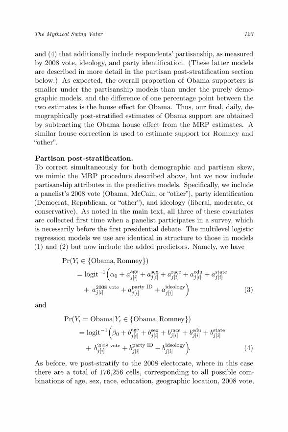
and (4) that additionally include respondents’ partisanship, as measuredby 2008 vote, ideology, and party identification. (These latter modelsare described in more detail in the partisan post-stratification sectionbelow.) As expected, the overall proportion of Obama supporters issmaller under the partisanship models than under the purely demo-graphic models, and the difference of one percentage point between thetwo estimates is the house effect for Obama. Thus, our final, daily, de-mographically post-stratified estimates of Obama support are obtainedby subtracting the Obama house effect from the MRP estimates. Asimilar house correction is used to estimate support for Romney and“other”.

Partisan post-stratification.To correct simultaneously for both demographic and partisan skew,we mimic the MRP procedure described above, but we now includepartisanship attributes in the predictive models. Specifically, we includea panelist’s 2008 vote (Obama, McCain, or “other”), party identification(Democrat, Republican, or “other”), and ideology (liberal, moderate, orconservative). As noted in the main text, all three of these covariatesare collected first time when a panelist participates in a survey, whichis necessarily before the first presidential debate. The multilevel logisticregression models we use are identical in structure to those in models(1) and (2) but now include the added predictors. Namely, we have

Pr(Yi 2 {Obama,Romney})




j[i]

+ a2008 votej[i] + aparty ID

j[i] + aideologyj[i]

⌘(3)

and

Pr(Yi = Obama|Yi 2 {Obama,Romney})



j[i] + bstatej[i]

+ b2008 votej[i] + bparty ID

j[i] + bideologyj[i]

⌘. (4)

As before, we post-stratify to the 2008 electorate, where in this casethere are a total of 176,256 cells, corresponding to all possible com-binations of age, sex, race, education, geographic location, 2008 vote,

124 Gelman et al.

party identification, and ideology. Since here we explicitly incorporatepartisanship, we do not adjust for the house effect as we did with thepurely demographic adjustment.

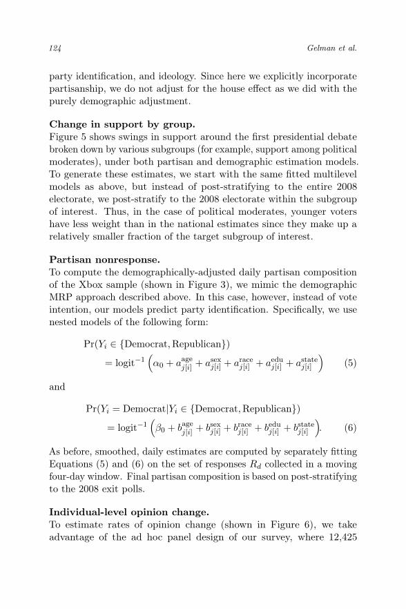
Change in support by group.Figure 5 shows swings in support around the first presidential debatebroken down by various subgroups (for example, support among politicalmoderates), under both partisan and demographic estimation models.To generate these estimates, we start with the same fitted multilevelmodels as above, but instead of post-stratifying to the entire 2008electorate, we post-stratify to the 2008 electorate within the subgroupof interest. Thus, in the case of political moderates, younger votershave less weight than in the national estimates since they make up arelatively smaller fraction of the target subgroup of interest.

Partisan nonresponse.To compute the demographically-adjusted daily partisan compositionof the Xbox sample (shown in Figure 3), we mimic the demographicMRP approach described above. In this case, however, instead of voteintention, our models predict party identification. Specifically, we usenested models of the following form:

Pr(Yi 2 {Democrat,Republican})




j[i]

⌘(5)

and

Pr(Yi = Democrat|Yi 2 {Democrat,Republican})



j[i] + bstatej[i]

⌘. (6)

As before, smoothed, daily estimates are computed by separately fittingEquations (5) and (6) on the set of responses Rd collected in a movingfour-day window. Final partisan composition is based on post-stratifyingto the 2008 exit polls.

Individual-level opinion change.To estimate rates of opinion change (shown in Figure 6), we takeadvantage of the ad hoc panel design of our survey, where 12,425


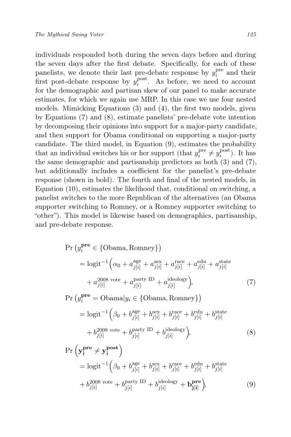
individuals responded both during the seven days before and duringthe seven days after the first debate. Specifically, for each of thesepanelists, we denote their last pre-debate response by ypre

i and theirfirst post-debate response by ypost

i . As before, we need to accountfor the demographic and partisan skew of our panel to make accurateestimates, for which we again use MRP. In this case we use four nestedmodels. Mimicking Equations (3) and (4), the first two models, givenby Equations (7) and (8), estimate panelists’ pre-debate vote intentionby decomposing their opinions into support for a major-party candidate,and then support for Obama conditional on supporting a major-partycandidate. The third model, in Equation (9), estimates the probabilitythat an individual switches his or her support (that ypre

i 6= yposti ). It has

the same demographic and partisanship predictors as both (3) and (7),but additionally includes a coefficient for the panelist’s pre-debateresponse (shown in bold). The fourth and final of the nested models, inEquation (10), estimates the likelihood that, conditional on switching, apanelist switches to the more Republican of the alternatives (an Obamasupporter switching to Romney, or a Romney supporter switching to“other”). This model is likewise based on demographics, partisanship,and pre-debate response.

Pr

�ypre

i 2 {Obama,Romney}�

= logit

�1⇣↵0 + aage



j[i]

+ a2008 votej[i] + aparty ID

j[i] + aideologyj[i]

⌘, (7)

Pr

�ypre

i = Obama|yi 2 {Obama,Romney}�

= logit

�1⇣�0 + bage


j[i] + bstatej[i]


j[i] + bideologyj[i]

⌘, (8)

Pr

⇣ypre

i 6= ypost

i

⌘

= logit

�1⇣�0 + bage


j[i] + bstatej[i]


j[i] + bideologyj[i] + bpre

j[i]

⌘, (9)

126 Gelman et al.

and

Pr

⇣ypost

i = more Republican alternative|ypre

i 6= ypost

i

⌘

= logit

�1⇣�0 + bage


j[i] + bstatej[i]


j[i] + bideologyj[i] + bpre

j[i]

⌘. (10)

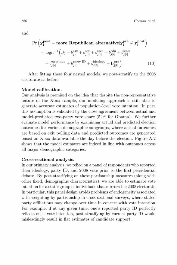
After fitting these four nested models, we post-stratify to the 2008electorate as before.

Model calibration.Our analysis is premised on the idea that despite the non-representativenature of the Xbox sample, our modeling approach is still able togenerate accurate estimates of population-level vote intention. In part,this assumption is validated by the close agreement between actual andmodel-predicted two-party vote share (52% for Obama). We furtherevaluate model performance by examining actual and predicted electionoutcomes for various demographic subgroups, where actual outcomesare based on exit polling data and predicted outcomes are generatedbased on Xbox data available the day before the election. Figure A.2shows that the model estimates are indeed in line with outcomes acrossall major demographic categories.

Cross-sectional analysis.In our primary analysis, we relied on a panel of respondents who reportedtheir ideology, party ID, and 2008 vote prior to the first presidentialdebate. By post-stratifying on these partisanship measures (along withother fixed, demographic characteristics), we are able to estimate voteintention for a static group of individuals that mirrors the 2008 electorate.In particular, this panel design avoids problems of endogeneity associatedwith weighting by partisanship in cross-sectional surveys, where statedparty affiliations may change over time in concert with vote intention.For example, if at any given time, one’s reported party ID perfectlyreflects one’s vote intention, post-stratifying by current party ID wouldmisleadingly result in flat estimates of candidate support.


Figure A.2: Comparison of election outcomes (estimated from exit poll data) toXbox predictions computed the day prior to the election. Despite being based on ahighly non-representative sample, the Xbox predictions are largely in line with theelection outcomes.

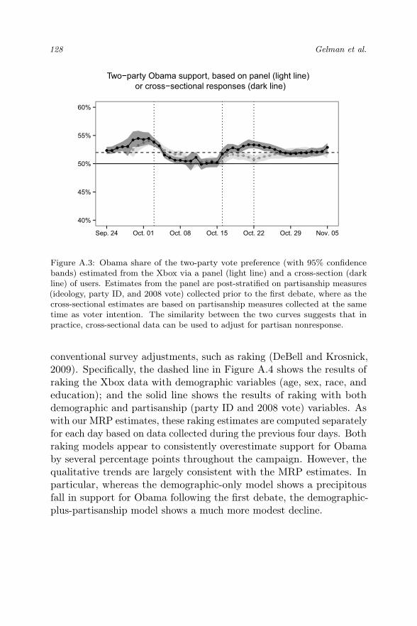
Nevertheless, despite the theoretical advantages of a panel analysis,cross-sectional data are often easier to collect. To check whether ourapproach can be applied to cross-sectional surveys, we limit our Xboxsample to the 327,432 first-time interviews — in which respondentssimultaneously provide both partisanship and vote intention informa-tion — and then correct for partisan nonresponse via MRP as before.That is, we discard all follow-up interviews, where only vote intentionwas collected. Figure A.3 shows that post-stratifying on the cross-sectionally reported partisanship measures yields similar results to thoseobtained via the panel analysis. Thus, to a large extent, partisan non-response can be detected and adjusted for even via a naive statisticalapproach that does not account for possible movements in reportedpartisanship.

Raking.MRP is a robust approach for identifying and correcting for partisannonresponse. Our qualitative findings, however, can also be seen with

128 Gelman et al.

40%

45%

50%

55%

60%


Two−party Obama support, based on panel (light line)or cross−sectional responses (dark line)

Figure A.3: Obama share of the two-party vote preference (with 95% confidencebands) estimated from the Xbox via a panel (light line) and a cross-section (darkline) of users. Estimates from the panel are post-stratified on partisanship measures(ideology, party ID, and 2008 vote) collected prior to the first debate, where as thecross-sectional estimates are based on partisanship measures collected at the sametime as voter intention. The similarity between the two curves suggests that inpractice, cross-sectional data can be used to adjust for partisan nonresponse.

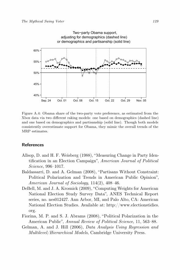
conventional survey adjustments, such as raking (DeBell and Krosnick,2009). Specifically, the dashed line in Figure A.4 shows the results ofraking the Xbox data with demographic variables (age, sex, race, andeducation); and the solid line shows the results of raking with bothdemographic and partisanship (party ID and 2008 vote) variables. Aswith our MRP estimates, these raking estimates are computed separatelyfor each day based on data collected during the previous four days. Bothraking models appear to consistently overestimate support for Obamaby several percentage points throughout the campaign. However, thequalitative trends are largely consistent with the MRP estimates. Inparticular, whereas the demographic-only model shows a precipitousfall in support for Obama following the first debate, the demographic-plus-partisanship model shows a much more modest decline.


40%

45%

50%

55%

60%


Two−party Obama support,adjusting for demographics (dashed line)

or demographics and partisanship (solid line)

Figure A.4: Obama share of the two-party vote preference, as estimated from theXbox data via two different raking models: one based on demographics (dashed line)and one based on demographics and partisanship (solid line). Though both modelsconsistently overestimate support for Obama, they mimic the overall trends of theMRP estimates.

References

Allsop, D. and H. F. Weisberg (1988), “Measuring Change in Party Iden-tification in an Election Campaign”, American Journal of PoliticalScience, 996–1017.

Baldassarri, D. and A. Gelman (2008), “Partisans Without Constraint:Political Polarization and Trends in American Public Opinion”,American Journal of Sociology, 114(2), 408–46.

DeBell, M. and J. A. Krosnick (2009), “Computing Weights for AmericanNational Election Study Survey Data”, ANES Technical Reportseries, no. nes012427. Ann Arbor, MI, and Palo Alto, CA: AmericanNational Election Studies. Available at: http://www.electionstidies.org.

Fiorina, M. P. and S. J. Abrams (2008), “Political Polarization in theAmerican Public”, Annual Review of Political Science, 11, 563–88.

Gelman, A. and J. Hill (2006), Data Analysis Using Regression andMultilevel/Hierarchical Models, Cambridge University Press.

130 Gelman et al.

Gelman, A. and G. King (1993), “Why Are American Presidential Elec-tion Campaign Polls So Variable When Votes Are So Predictable?”,British Journal of Political Science, 23(04), 409–51.

Gelman, A. and T. C. Little (1997), “Poststratification into Many Cate-gories Using Hierarchical Logistic Regression”, Survey Methodology.

Ghitza, Y. and A. Gelman (2013), “Deep Interactions with MRP: Elec-tion Turnout and Voting Patterns Among Small Electoral Sub-groups”, American Journal of Political Science, 57(3), 762–76.

Gutsche, T., A. Kapteyn, E. Meijer, and B. Weerman (2014), “TheRAND Continuous 2012 Presidential Election Poll”, Public OpinionQuarterly.

Hillygus, D. S. and S. Jackman (2003), “Voter Decision Making in Elec-tion 2000: Campaign Effects, Partisan Activation, and the ClintonLegacy”, American Journal of Political Science, 47(4), 583–96.

Himmelweit, H. T., M. J. Biberian, and J. Stockdale (1978), “Memoryfor Past Vote: Implications of A Study of Bias in Recall”, BritishJournal of Political Science, 8(03), 365–75.

Kaminska, O. and C. Barnes (2008), “Party Identification Weighting:Experiments to Improve Survey Quality”, in Elections and ExitPolling, NJ, Wiley Hoboken, 51–61.

Kaplan, N., D. K. Park, and A. Gelman (2012), “Polls and ElectionsUnderstanding Persuasion and Activation in Presidential Campaigns:The Random Walk and Mean Reversion Models”, Presidential Stud-ies Quarterly, 42(4), 843–66.

Lax, J. R. and J. H. Phillips (2009), “How Should We Estimate PublicOpinion in the States?”, American Journal of Political Science, 53(1),107–21.

Levendusky, M. (2009), The Partisan Sort: How Liberals becameDemocrats and Conservatives became Republicans, University ofChicago Press.

Little, R. J. A. (1993), “Post-stratification: A Modeler’s Perspective”,Journal of the American Statistical Association, 88(423), 1001–12.

Reilly, C., A. Gelman, and J. Katz (2001), “Poststratification WithoutPopulation Level Information on the Poststratifying Variable WithApplication to Political Polling”, Journal of the American StatisticalAssociation, 96(453).

Sides, J. and L. Vavreck (2014), The gamble: Choice and Chance in the2012 Presidential Election, Princeton University Press.

the mythical swing voter - columbia universitygelman/research/published/swingers.pdf · the...

Documents