Darwin College Research Report DCRR-005

The Intertemporal Approach to the Current Account and Currency Crises

Sergejs Saksonovs

June 2006

Darwin College Cambridge University United Kingdom CB3 9EU www.dar.cam.ac.uk/dcrr

ISSN 1749-9194

The Intertemporal Approach to the CurrentAccount and Currency Crises

Sergejs Saksonovs

Faculty of Economics

University of CambridgeJune 2006

Abstract

This paper investigates the relationship between optimal current account deficitsand currency crises. The framework for determining the optimal size of the currentaccount is the intertemporal approach. The intertemporal model of the currentaccount is empirically estimated for a sample of 17 countries, ten of which didexperience a currency crisis (broadly defined).

Given the large number of countries analyzed under a single set of restrictiveassumptions, the intertemporal model of the current account performed well, oftencapturing important dynamics in the data. In five cases current account levelsdeviated substantially from the optimal level before the occurrence of the currencycrisis, showing that the intertemporal approach has some predictive power for thecurrency crises. Finally, there was no evidence for countries being unable to runoptimal current accounts because of lack of access to the world financial marketsin the aftermath of the crisis.

1 Introduction

Current account deficits have been observed in a variety of countries over time. In thelast several decades two tendencies - gradual removal of trade barriers and increasedfreedom of international capital flows have made it easier for countries to engage ininternational trade and borrowing or lending across the borders. During the same time,however, there has been “pervasive currency turmoil” in the aftermath of the collapse ofthe Bretton Woods system and later a series of currency crises in the nineties (Kaminskyand Reinhart, 1999). According to Edwards (2001), “currency crises of the 1990s shockedinvestors, academics, international civil servants and policy makers”. Efforts to explainthese developments motivate increased attention to the modeling of the dynamics ofcurrent accounts for different countries.

The link between the current account and the potential of the currency crisis lies inthe fundamental insight that no country is able to accumulate foreign debt (run a currentaccount deficit) indefinitely. If the current account deficit at some point becomes unsus-tainable, then a currency crisis - an adjustment to a surplus through a rapid depreciationof the domestic currency is possible. The key characteristic of the current account deficitsis therefore their sustainability not their size. Countries that run large current accountdeficits do not necessarily end up having currency crises. In order to assess sustainabilityof the current account deficits, a theoretical framework of analysis is required.

One possible approach to analyzing current account deficits is to view them as adifference between saving and investment flows. A prime example of a country with largecurrent account deficit, which so far has been sustainable, is the United States. Bernanke(2005) explains the US current account deficit by the hypothesis of the ‘saving glut’,which states that the current deficit is responding to the inflow of surplus world saving,which caused favorable shocks to the stock prices and the interest rate. Similarly, forCooper (2001) the growing US current account deficit is a vote of confidence by the restof the world in claims on Americans. Mann (2002), on the other hand, concludes thatan adjustment to smaller levels of the current account deficit is inevitable and is likely tooccur either through dollar depreciation or structural changes within the United States,including an increase in the domestic saving by the US residents.

The prevalent theoretical framework for studying the dynamics of the current accountis the intertemporal approach, which views current account as a change in the net foreignasset position of a country. The intertemporal approach is founded on utility maximizingdecisions by economic agents. Therefore it provides a better way to judge sustainabilityof the deficits than an approach based on aggregate relationships between saving andinvestment flows. Large deficits according to the intertemporal approach can be optimaland sustainable and therefore not a cause of concern for policymakers.

The contribution of this paper is to use the empirical method of Bergin and Shef-frin (2000) to test the intertemporal current account model for 17 of countries, some ofwhich did experience currency crises and some of which did not. Empirical tests of theintertemporal models of current account behaviour have been fewer than the amount oftheoretical literature on the topic (Kasa, 2003). Calderon et al. (2000) also mentions thatstudies empirically analyzing the effect of macroeconomic variables on current accountdeficits are few compared to the importance frequently attached to the current accountby policymakers.

1

This paper also considers two hypotheses regarding the relationship between currentaccount deficits and currency crises. Firstly, if one observes a significant deviation ofthe current account levels from the ones predicted by the intertemporal model, whichdescribes the optimal evolution of the current account, it could serve as a signal of un-sustainable deficits. This is true, if one assumes that the optimal path for the currentaccount is also sustainable. Therefore intertemporal models of current account could havepredictive power for currency crises.

Secondly, one of the crucial assumptions of the intertemporal approach is the ability ofthe country to borrow at the prevalent ‘world interest rate’ - that is a country is assumedto have unlimited access to international financial markets. In the aftermath of a crisis,access to international financial markets may be impeded, due to foreign investor fears.This can be tested by assessing the fit of the intertemporal approach for such countriescompared to the countries which have not experienced a crisis.

Section 2.1 explains the fundamental implications of the intertemporal approach tothe current account. Section 2.2 formulates a testable implication of the model that theempirical analysis is based on. Section 3 describes the data collection and assumptionsmade for fitting the model. Section 4 shows the results of the empirical analysis anddiscusses its limitations and Section 5 provides conclusions and directions for futureresearch.

2 Theory of the Intertemporal Approach

2.1 The Intertemporal Approach to the Current Account

Originally the current account was thought of as the net export balance of a country.Consequently, relative international prices and their determinants were viewed as centralto the dynamics of the current account. The alternative viewpoint emphasized that thecurrent account is also the difference between saving and investment and focused onmacroeconomic factors that determine these two variables. The intertemporal approachto the current account recognizes that saving and investment decisions result from forwardlooking calculations based on the expected values of various macroeconomic factors. Itachieves a synthesis between the trade and financial flow perspectives by recognizinghow macroeconomic factors influence future relative prices and how relative prices affectsaving and investment decisions (Obstfeld and Rogoff, 1995).

Obstfeld and Rogoff (1995) separate the intertemporal current account models intotwo broad groups - deterministic and stochastic. Deterministic models operate underthe assumption of perfect foresight of relevant variables and complete information. Thebasic model postulates that a representative consumer maximizes a time separable utilityfunction:

U =∞∑

t=0

βu(Ct) (2.1)

The consumer is discounting the value of future utility (0 < β < 1), and the marginalutility of private consumption at the end of period t - Ct is always positive (u′(Ct) > 0),but decreasing (u′′(Ct) < 0).

2

The next step involves specifying the resource constraint for the economy. At the endof period t the economy produces domestic output Yt and receives income on existing netforeign assets At

1 with an interest rate rt between periods t−1 and t. The received incomeis spent on private sector consumption Ct, government consumption Gt, net investmentIt and potentially acquisition of more foreign assets. Recalling that the current accountis defined as the change in net foreign assets, one can write:

CAt = At+1 − At = rtAt + Yt − Ct −Gt − It (2.2)

Following Obstfeld and Rogoff (1995), one can define the market discount factor at datet for the consumption at a future date k (k > t), which accounts for the variable interestrate as follows:

Rt,k =1∏k

i=t+1(1 + ri)(2.3)

The intertemporal approach expresses the current account in deviations from ‘perma-nent’ levels of variables. A ‘permanent’ level of variable Z at time t is defined as:

Zt =

∑∞k=t Rt,kZk∑∞

k=t Rt,k

(2.4)

In particular, the ‘permanent’ relationship between the market and consumer’s discountrates can be defined as:

(β

R

)σ

=

∑∞k=t Rt,k

(βk−t

Rt,k

)σ

∑∞k=t Rt,k

(2.5)

Appendix A uses (2.2) to derive the following equation describing the current accountbehaviour as a deviation of macroeconomic variables from their permanent levels:

CAt = (rt−rt)At+(Yt−Yt)−(It−It)−(Gt−Gt)+

1− 1

(βR

)σ

(rtAt+Yt−It−Gt) (2.6)

Equation (2.6) is the key insight of the intertemporal approach. The first four termsreflect consumption smoothing processes in the economy. For the example, if the worldinterest rate is higher than the permanent level and the country is net foreign creditor(At > 0), the current account will increase as agents smooth the effects of temporarilyhigher interest income on foreign assets. Similarly, agents will smooth the effects ofan increased output above its permanent level, while they will use foreign borrowing(decreasing the current account) to smooth the effects of temporarily high investment orgovernment spending.

The final term in (2.6) reflects consumption tilting. Consumption tilting arises dueto the difference between world real interest rate and domestic rate of time preference.

If the home country is on average more impatient than the rest of the world, then(

βR

)σ

will be less than 1 and there will be a tendency to the decrease in the current account,

1There is debate about accounting net foreign asset positions. Hausmann and Sturzenegger (2006)argue that net foreign assets should be valued on the basis of their returns rather than their historicalcosts. The majority of literature, however, including this paper, uses cost basis.

3

that is proportional to the ‘permanent’ values of economy’s resources. If the domesticeconomy is more patient, then the reverse effect occurs (Obstfeld and Rogoff, 1995).

It is possible to extend this basic framework, by introducing production function andcapital accumulation, comparative advantage (expressed in different time preferences ofconsumers in different countries), accounting for non-tradable and durable goods, etc.However, (2.6) is the starting point for formulating testable implications of the intertem-poral approach.

One important caveat of (2.6) is that it describes the current account when there iscomplete certainty. Stochastic models of the current account introduce uncertainty overthe changes of relevant macroeconomic variables. As Obstfeld and Rogoff (1995) pointout, the key consideration in introducing uncertainty is the extent to which agents caninsure themselves against unpredictable contingencies (e.g. output fluctuations that aresubject to random shocks).

One extreme way of introducing uncertainty is to introduce the finite number ofstates of the world with known characteristics and the existence of markets to tradegoods contingent on the occurrence of a particular state (Arrow-Debreu securities). Inthis case, one can analyse the model, as if no uncertainty existed, but rather the numberof goods has been increased to include all possible contingencies. An intermediate optionis to introduce partially complete markets, where incompleteness stems from asymmetricinformation at the micro level (Obstfeld and Rogoff, 1995). A polar opposite of theArrow-Debreu setup, is to postulate the existence of a single traded asset. This is theframework used in this paper. The insights of such a model are qualitatively similarto the deterministic model, except that the relevant variables are now replaced by theirexpectations.

2.2 The Testable Hypothesis of the Intertemporal Approach

For the empirical analysis of the current account (2.6), which includes non-observablefactors, has to be made operational. In the simplest case, one can assume that there are nodivergences between the world real interest rate and the subjective rate of time preference,thereby eliminating the consumption tilting term of the (2.6). The main problem is tofind the permanent values of output, investment, government consumption and interestrate, or, in the case of a model with uncertainty, their expectations. Information onexpectations over a wide variety of countries and time periods is generally not availableto the analyst (Ghosh, 1995).

The solution in the literature has been to use the methodology developed for testingpresent value models by Campbell and Shiller (1987). In context of the current account,the idea is that under the null hypothesis of the intertemporal approach to the currentaccount, the history of the current account includes the information agents have aboutthe values of relevant macroeconomic variables, which might not otherwise be observableto the analyst.

Ghosh (1995), Otto (1992) and others have tested the intertemporal approach to thecurrent account for various countries. The general results of these early tests have notbeen encouraging. The predicted current account series were typically far less volatilethan the actual data and failed to capture important dynamics in the data. To improvethe results, the tests were extended to relax some assumptions. One way is to relax the

4

assumption of a constant real interest rate equal to the rate of time preference. Berginand Sheffrin (2000) allow for a variable interest rate and also extend the baseline modelto account for the existence of tradable and non-tradable goods and the variation in therelative prices of non-tradable goods. This is the theoretical justification for the factthat the current account should be responsive to exchange rate shocks. They achieve amarked improvement for countries, where previously the results were problematic. Thispaper uses the method of Bergin and Sheffrin (2000) to test the intertemporal approachacross different countries, firstly, because it has improved results, and, secondly, becauseit takes into account the variations in the exchange rate, which is important in contextof the currency crises.

In order to incorporate the distinction between traded and non-trade goods, Berginand Sheffrin (2000) modify the instantaneous utility function to be:

u(CT , CN) =(Ca

T C1−aN )1−σ

1− σ(2.7)

A new parameter a is the share of traded goods in private final consumption (CT is theconsumption of traded goods and CN is the consumption of non-traded goods). Undercertain assumptions on distributions of stochastic variables, Bergin and Sheffrin (2000)derive a version of the Euler equation:

Et∆ct+1 =1

σEtrt+1 (2.8)

where ∆ct+1 = log Ct+1− log Ct, 1/σ is the intertemporal elasticity of substitution and ris ‘consumption-based’ interest rate defined as follows:

rt = rt +

[1− 1

σ1σ

(1− a)

]∆pt + η (2.9)

In (2.9), pt is the log of the relative price of non-traded goods in terms of traded goods.In this way, one can include the effects of variable interest rates and relative prices. Theconstant term η, consists of variances and covariances of interest rate, consumption andrelative prices of traded goods and can be disregarded, when the model is fitted usingthe demeaned series.

The key testable implication of the intertemporal approach is obtained by linearizingthe intertemporal budget constraint around the steady state in which the net foreignassets are equal to zero. Appendix B shows that after log-linearizing the intertemporalbudget constraint, taking expectations and using (2.8), one can obtain:

CAt = −Et

∞∑i=1

βi(∆not+i − 1

σrt+i) (2.10)

where not is the log of ‘net output’ (defined as: Yt− It−Gt) and CAt is the value of thecurrent account predicted by the model.

To generate expected values of relevant macroeconomic variables, following Berginand Sheffrin (2000), the following vector autoregression model is used.

∆not

CAt

rt

=

β11 β12 β13

β21 β22 β23

β31 β32 β33

∆not−1

CAt−1

rt−1

+

ε1t

ε2t

ε3t

(2.11)

5

Equation (2.11) in matrix notation can be written as: yt = Ayt−1 +ut, which means:Etyt+i = Aiyt. Furthermore, using appropriate vectors one can write (2.10) in matrixnotation using (2.11):

CAt = −∞∑i=1

βi

(l1 − 1

σl2

)Aiyt

where l1 =[1 0 0

]and l2 =

[0 0 1

]. Assuming that the processes in yt are stationary

(Campbell and Shiller, 1987), the infinite sum in the equation (2.10) will converge asfollows:

kyt = −(l1 − 1

σl2

)βA(I− βA)−1yt (2.12)

The testable implication is that, assuming the intertemporal approach holds, the esti-mated vector k should be equal to

[0 1 0

]. The equation (2.12) allows obtaining the

value of the current account implied by the restrictions of the intertemporal model. Thispredicted value can be compared with the actual data both visually and formally.

For every country this paper performs a VAR estimation with one lag to obtain thematrix A and subsequently the vector k according to the equation (2.12) together withtheir standard errors. By delta method the variance covariance matrix of the vector kelements is given by: (∂k/∂A)V(∂k/∂A)′, where V is the 9 × 9 variance covariancematrix of the estimated VAR parameters, and ∂k/∂A is a 3 × 9 matrix containing thederivatives of the k vector with respect to the VAR parameters.

Apart from simple statistical tests on the significance of estimated elements of vectork, this paper uses two other informal criteria to assess the overall performance of themodel. The first is the variance ratio between the predicted and actual current accountseries. This is motivated by the repeated finding in the literature (for example, Ghosh(1995) or Bergin and Sheffrin (2000)) that modeled current account series often exhibitlesser volatility than the actual data. The second criteria is the root mean square errorbetween the modeled current account series and the actual data.

However, it is also desirable to have a way to jointly assess the restrictions of themodel. Theoretically a simple Wald test of the non-linear restriction on the vector kimplied by (2.12) is appropriate. However, as Mercereau and Jacques (2004) show thereare problems with this method due to the possible near singularity of the matrix (I−βA).A test that is not affected by this issue can be derived by multiplying vector k by thematrix (I−βA) and testing the corresponding linear restriction instead of the non-linearone.

Campbell and Shiller (1987) show that these tests are equivalent, although the Waldtest statistics will not be the same. Adapting the method by Campbell and Shiller (1987)and Mercereau and Jacques (2004), one can define Rt = CAt−CAt−1/β−∆not +(1/σ)rt

and regress it on the lagged values of CAt, ∆not and rt. The test that is equivalent to thenon-linear restriction in (2.12), is then simply the test of the joint nullity of the regressioncoefficients.

3 Data Collection and Series Analysis

There are 17 countries in the sample used in this paper - Australia, Canada, France,Germany, Italy, Japan, Korea, Mexico, Netherlands, Norway, Philippines, South Africa,

6

Spain, Sweden, Switzerland, United Kingdom and the United States. All countries arecurrently economies that are fairly open to and involved in international trade. The maincriteria for choosing the sample was the availability of comparable, quarterly data for asufficiently large period. Annual observations were not used for three reasons. First,there is generally larger uncertainty about annual estimates (Bergin and Sheffrin, 2000).Second, there are concerns about the performance of the empirical method on smallsamples (Mercereau and Jacques, 2004). Finally, annual observations would not allowclose analysis of the before and after crisis situations. To ensure a sufficient number ofobservations, only the series that had started before or on 1981 were chosen.

The first parameter, which is fundamental to the model, is the ‘world real interestrate’. This value is to an extent an abstraction, which needs to be substituted by asuitable proxy. Similarly to Bergin and Sheffrin (2000), this paper follows the methodof Barro and Sala i Martin (1990). First, quarterly nominal interest rate series of G7member countries were collected. T-bill rate or money market rate series from IFS wasused as a measure of benchmark nominal real interest rate series. To deal with missingobservations, for some countries the euro area series was used (from 1999 to 2005).

Second, data on inflation was computed using the quarterly CPI series from IFS2.Inflation expectations were then computed with an autoregression for six quarters. Tofind the real interest rate, inflation expectations were subtracted from the nominal interestrate for each country. Unfortunately, this method can be problematic for the periods ofhigh inflation in all G7 economies, such as the end of the seventies, because the computedreal interest rate turns out to be substantially negative for those periods.

Finally, to compute the ‘world real interest rate’ from the real interest rates of G7economies, a real GDP weighted average is used. Real GDP in dollars is obtained fromthe World Bank Development Indicators database3. The ‘world real interest rate’ seriesis used to construct the consumption based interest rate according to (2.9) and is thesame for all of the countries in the sample.

The parameter β is set to be equal to 1/(1 + rw), where rw is the mean for thecalculated world real interest rate. This does not imply that there is no consumptiontilting for an individual country, but rather that there is no consumption tilting overtime and across countries on average. The value of β is equal to 0.98.

Regarding a - the share of traded goods in the private final consumption, Bergin andSheffrin (2000) cite two empirical studies which produce the estimates of a ≈ 1/2 anda ≈ 2/3. Their results do not depend significantly on the choice of the coefficient anda less generous estimate of a = 1/2 is chosen. This coefficient is likely to be slowlyincreasing over time as international trade becomes easier and new traded goods (forexample, software) emerge. However, counteracting this trend could be the growingimportance of services in consumption.

The parameter σ can be interpreted as the coefficient of relative risk aversion forthe utility function used in (2.7). More relevant for estimating (2.9) is the value of1/σ interpreted as the intertemporal elasticity of substitution. Although these measuresshow as reciprocals due to the nature of the utility function, they are distinct and Berginand Sheffrin (2000) cite mutually exclusive estimates of σ and 1/σ. Bergin and Sheffrin(2000) find that the model performs best with low values of intertemporal elasticity of

2Adjusted West Germany country series were used to determine Germany CPI from 1975 to 1990.3Since the GDP is the annual series, the weights also change annually.

7

substitution, in line with the existing empirical estimates of about 0.1. The value of1/σ is set to 0.1 for all countries in order to identify whether there are tendencies in thefit of the model that do not depend on differing consumer preferences for intertemporalsubstitution.

For the price of the non-traded goods in terms of traded goods - Pt in (2.9), this paperuses a measure of the real exchange rate as a proxy. The real exchange rate series is takenfrom the OECD Main Economic Indicators database. OECD real effective exchange ratemeasure is based on a principle which takes into account relative market shares heldby country’s competitors on the common markets, including the home market, and theimportance of these markets for the country in question (OECD, 2006)4. Six quarterautoregression is used to generate expected values of the exchange rate. With the valuesof rt, 1/σ, a and Pt one can construct the rt, consumption based interest rate seriesaccording to (2.9) for every individual country.

The OECD Main Economic Indicators database provides the data on deflated GDPcomponents for the majority of the countries in the sample. For the countries, whereOECD data was not available for the sufficiently large period (Germany, Japan andthe Philippines) the IFS series were used, adjusted by the GDP deflator. Since one ofthe fundamental implications behind the intertemporal approach is the framework ofa working representative agent, the series were converted on a per unit of labor forcebasis. Data on labor force was obtained from the OECD Main Economic Indicators or,where unavailable, from the World Bank Development Indicators. The OECD definitionof labour force includes all persons who fulfil the requirements for inclusion among theemployed or the unemployed during a specified reference period.

The net output series was calculated as the difference between GDP and gross fixedcapital formation combined with government consumption expenditure per unit of labourforce. The logged and differenced series was termed ∆not. The current account measureCAt was obtained by subtracting the log of per labour force consumption from the logof the net output. All three series rt, ∆not and CAt are used in their demeaned form,which means that the focus is on checking the dynamic implications of the model.

4 Results

4.1 Stationarity Tests

There are three reasons to perform stationarity tests on the series. First, under theassumption of rational expectations, (2.10) implies that the current account should be alinear combination of the stationary series (Trehan and Walsh (1991) also link stationarityand budget constraints). Second, stationarity of all three series is required for the infinitesum to converge as in (2.12). Third, series used in VAR estimated by the OLS need tobe stationary.

To check that the series used in the estimation of VAR are stationary, both thePhillips-Perron test statistic and the augmented Dickey-Fuller test statistics are reported

4This series was not available for South Africa and the Philippines. For these countries, the nominalexchange rate index from IFS was used and adjusted by the ratio of the home country’s CPI and CPI ofthe industrial countries.

8

as well as their accompanying p-values for the null hypothesis that the series containsa unit root. Since the series are used in their demeaned form, test regressions do notinclude a constant and time trends.

Table 1 summarizes the results of the two unit root tests on all three series used inthe model. Two of the series, differenced net output ∆not and consumption based realinterest rate rt, do not present any problems with both tests strongly rejecting the null ofthe unit root in all cases. The situation is different with the current account series CAt.In most cases tests can only reject the null of the unit root at 10% and in some cases oneof the tests fails to reject the null of the unit root at all. The demeaned current accountsdo not exhibit any apparent trends, therefore a simple detrending procedure does notremove the non-stationarity.

Earlier empirical estimation of intertemporal models, (e.g. Ghosh (1995)), had prob-lems establishing stationarity and Hall et al. (1999) establish a procedure to identifyperiodic non-stationarity in current account series, which they link with an increasedprobability of a crisis event. It is also well documented that classical unit root testshave low power against stationary, but slowly mean reverting alternatives. This becomesparticularly relevant for the countries, which have exhibited a strong tendency towardscurrent account surplus or current account deficits closer to the end of the sample, forexample, Australia, with its rising current account deficits during the last several years.

The threshold for considering series to be stationary was set low because of theseissues. If at least one test was able to reject the null hypothesis at 10% significance level,the series was considered stationary. However, given that such a variety of countries isconsidered in the study, it has been impossible to find a suitably large period, duringwhich all of the country current account series would be stationary.

4.2 Results for the Non-crisis Countries

The group of countries, which did not suffer a crisis, includes Australia, Canada, Japan,Germany, Netherlands, Switzerland and the United States.

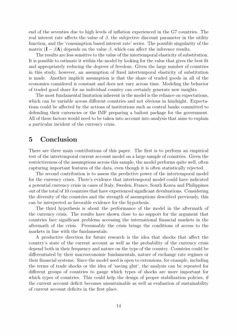
Table 3 shows the results for the panel of non-crisis countries. The first three columnsshow the estimated elements of k vector. The next columns list the number of obser-vations in the sample, the variance ratio of the predicted current account series to theactual data, the root mean square error (RMSE) of the fit and, finally, a test statistic totest the joint restrictions of the model, which is distributed as χ2 with three degrees offreedom, and it’s p-value.

The elements of the k vector that the theory predicts to be zero (kno and kr) arenever significantly different from zero. In six cases out of seven the estimated valueof kCA, which theory predicts to be one, is significantly different from zero, with theonly exception being Australia. In four cases out of those six the estimated coefficientswere not significantly different from one. One interesting exception was Japan, whoseestimated value of kCA was equal to 3.349 and significantly different from unity.

In three cases, the model predicts a much more volatile current account series thanactually exhibited, which is rare across the sample. The three cases are Japan, Switzer-land and the United States. A plausible explanation is that the assumed value of theintertemporal elasticity of substitution is very different from the actual preferences of theconsumers. Japan, for example, had historically high levels of domestic saving, whereas

9

the United States had the opposite situation. The average ratio of the predicted vari-ance to actual variance in the developed countries is equal to 4.72, although this value issignificantly distorted by three cases mentioned above.

The average RMSE of the prediction is equal to 0.029. For comparison, the infor-mation about the means and standard deviation of the current account series is givenin Table 2. One can see, that the prediction RMSE is roughly equal in the order ofmagnitude to the standard deviations of the current account series. The best fit of themodel is achieved in the case of Germany, whereas the worst, significantly enough, in forthe United States.

The test statistics for the overall restrictions of the model generally reject the nullhypothesis of the intertemporal approach being true at 10%. The only exception isAustralia. However, the estimates for Australia are far from their theoretical values, whichsuggests that the failure to reject the null is due to the uncertainty of the estimates ingeneral. The null is most strongly rejected in cases of Switzerland and the United States,two countries, which also had more volatility in the predicted series than in the actualvalue.

The United States, given the importance of its current account deficit, is a particularlyimportant case. Since the predicted deficit is larger than the actual one, it can serve asevidence that concerns about the current account deficit in the US are misplaced andthat the viewpoints of Bernanke (2005) or Cooper (2001) reflect reality. However, sincethe model relies on expectations, it is also possible that it simply reflects the status quoarrangements, where the US had no trouble financing its current account deficit. Thissituation may change due to forces not included in the model.

4.3 Results for the Crisis Countries

The crisis of the European Monetary System (EMS) has been a predecessor to the cur-rency crises in Latin America and Asia. Eichengreen (2000) identifies the main countriesthat suffered during the EMS crisis - Italy, United Kingdom and to a lesser extent Spain,Sweden, France and Norway.

Sachs et al. (1996) reviews currency crises involving currency devaluation and thedepletion of currency reserves. Several countries from the sample of this paper are men-tioned in his study - Mexico (for the notable crisis in December 1994), Korea, which wasalso later affected by the Asian crisis, Philippines and South Africa. The crisis countriestherefore are France, Italy, South Korea, Mexico, Norway, South Africa, Philippines,Spain, Sweden and United Kingdom.

Table 4 summarizes the results of the estimation for the group of the crisis countries.Again, the first three columns report elements of the k vector. As in the case of healthycountries kno and kr are never significantly different from zero. The kCA coefficient isnot significantly from zero only for the Philippines. The standard error of the estimatedcoefficient on the current account of the Philippines is too large and the coefficient cannotbe distinguished from either zero or one.

Among the nine countries, whose estimated values of kCA are significantly differentfrom zero, in three cases the coefficient is not significantly different from unity giving thebest match between theory and data - Mexico, South Africa and the United Kingdom. Inthe remaining six cases, three countries have the values of kCA that are between zero and

10

unity and significantly different from both of those values. The interesting exceptionsare Sweden and France, where the estimated values of kCA are negative and significantlydifferent from zero.

On average among the crisis countries the model generates current accounts that areabout half as volatile as the actual data. There are only two instances where the volatilityof the predicted series slightly exceeds the actual volatility - South Africa and the UnitedKingdom, which are also the countries with best fits of the predicted series.

The average root mean square error of the prediction is equal to 0.029, which is thesame as for the panel of healthy countries. This means that if the currency crisis exhibitsany effects on the fit of the intertemporal model to the current account, they are toosmall to be felt in the context of the large sample of several decades. France and Swedenexhibit the worst fit of the model (being the only two countries where the sign of kCA isnegative), whereas South Africa and the United Kingdom show the best fits.

The test for the overall model restrictions cannot reject at 10% the null of the in-tertemporal approach being true in the case of France, Italy, South Africa, Spain and theUnited Kingdom. For France it is again the general uncertainty over values that does notlet the null to be rejected. South Africa and the United Kingdom, however, are clearlythe most successful instances of the model over both healthy and crisis countries.

4.4 Current Accounts before and after the Crisis Events

To analyse the fit around the time of the currency crisis it is necessary to first define thepoint of the crisis. According to Eichengreen (2000), who provides an overview of theEMS crisis, Italy and the United Kingdom devalued and left the exchange rate mechanism(ERM) in the third quarter of 1992. In the fourth quarter of 1992, Sweden and Norwayalso abandoned the ERM. Spain devalued twice with the larger devaluation occurring inthe second quarter of 1993. At the same time France also struggled with the impendingdevaluation.

Sachs et al. (1996) review the crises in the developing countries. One of the mostsignificant events is the crisis in Mexico, in the last quarter of 1994. South Korea andPhilippines, which Sachs et al. (1996) find vulnerable, were a part of the East Asiancurrency crisis with the main devaluations in the last quarter of 1997. Finally, SouthAfrica, which was frequently mentioned in the literature (e.g. Sachs et al. (1996) andFurman et al. (1998)) as vulnerable to a currency crisis had suffered from a speculativeattack in the first quarter of 1996 (Aron and Elbadawi, 1999).

These time points will be used to investigate the performance of the intertemporalmodel of current account before and after the crisis. The fact that the average root meansquare errors over the whole of the period in question are generally the same suggeststhat currency crises will generally have a short-term effect on the fit of the intertemporalmodel. Therefore, to see the usefulness of the intertemporal approach as a predictor ofthe currency crisis, the estimated current account series and the actual current accountfor two years (eight quarters) before the crisis point are compared. In addition, theperformance of the model for two years after the crisis is assessed to see whether thecurrency crisis had affected the ability of the country to access the international financialmarkets.

Figures 1 through 9 present the performance of the intertemporal current account

11

model for the countries that have experienced a crisis in chronological order. In additionthe root mean square error is reported both for the two years before the crisis and thetwo years after the crisis.

The first two countries are Italy and the United Kingdom. Figure 1 shows that beforethe Italian devaluation, Italy was running a current account deficit, which was higherthan the one predicted by the model. After the crisis, the current account switches tosurplus and again it’s higher than the one predicted by the model. The RMSE beforethe crisis point is more than three times than that after the crisis point, suggesting thatmodel’s performance improves after the crisis. This confirms the hypothesis that theintertemporal approach can have predictive power, but provides evidence against creditconstraints in the aftermath of the crisis.

Figure 2 shows that the United Kingdom does not have a similar pronounced effect,the actual current account deficit is lower than the predicted one before the crisis. Thispresents evidence against both of the hypotheses.

Figures 3 and 4 show the situation in Sweden and Norway respectively. Figure 3shows that Sweden has been running a current account deficit before the crisis, when themodel was a predicting a surplus. The RMSE of the model is seven times higher beforethe crisis than afterwards. Norway (Figure 4), however, shows that the model performsbetter before the crisis point than afterwards. At the point of the crisis Norway is runninga higher current account surplus than predicted by the model.

Figure 5 shows that the predicted current account deficit for Spain was higher than theactual one before the crisis. Again, the RMSE before the crisis is higher than afterwards,similar to the case of Sweden and Italy. France (Figure 6) was running a deficit instead ofthe predicted surplus before the crisis, however, the RMSE is virtually unchanged bothbefore and after the crisis.

Figure 7 shows that the intertemporal model fits Mexico very well even around theperiod of the crisis, similarly to the United Kingdom. The RMSE does not changesignificantly before or after the crisis. Figure 8 shows that the model also tracks SouthAfrican current account quite well around the time of the crisis (slightly overpredictingthe deficit).

Figure 9 shows that Korea has been running a deficit much higher than the onepredicted by the model and then similarly to Italy a higher surplus. The RMSE of themodel decreased after the crisis. Similarly, the Philippines (Figure 10) also ran a higherthan predicted current account deficit before the crisis. The RMSE again decreased afterthe crisis.

One can therefore conclude that while there’s diversity of results, the model does ap-pear to have some predictive power for the currency crises, confirming the first hypothesisof this paper. The fact that it does not do so for all countries may suggest several differ-ences in the nature of currency crises that are not accounted for in this paper. First, thecrises that are not predicted by the model can arise not due to the current account deficitthat is not optimal, but rather due to adjustment to different equilibrium determined bychanging fundamentals. Second, this may be an evidence of the ‘tequila effect’ describedby Sachs et al. (1996), who argues that crises tend to spread affecting countries that arevulnerable to them. It is possible, that some instances of the currency crisis, for example,Norway were not due to the dangerous imbalance of the current account, but simply dueto the overall panic in the financial markets.

12

The other possible explanation is that the assumptions underlying the estimation aretoo restrictive and that there are significant differences between preferences and condi-tions in individual countries. For example, the intertemporal elasticity of substitution,the share of traded goods can differ.

The RMSE of the model generally falls after the crisis suggesting that in some in-stances the crisis did bring the current account closer to the optimum and that thereis no evidence of countries facing significant borrowing constraints on the internationalfinancial markets in the aftermath of the crisis. The reason for that could be the fact thatthe crisis does represent a process of adjustment, bringing financial markets (includingconditions of access) in line with the economic fundamentals. Therefore, after the crisisthere is no reason for credit constraints, since the changed fundamentals are now reflectedin the exchange rate or other financial variables.

4.5 Forecasts for Non-stationary Current Accounts

Out of 17 countries in the sample, 8 countries have had their sample shortened in orderto make the current account series stationary (shown in bold in Table 1). These countriesare Australia, France, South Korea, Netherlands, Philippines, South Africa, Sweden andthe United Kingdom. Four years was the maximum amount of observations that wasremoved, typically it was enough to remove one or two years.

It is first useful to find out whether the non-stationarity is associated with the currentaccount surpluses or current account deficits. The countries that have non-stationarycurrent account deficits are Australia, France, South Africa and the United Kingdom.Figures 11, 12, 13 and 14 show the mean forecasted values of the current account as wellas the confidence intervals (+/- 2 standard deviations). Only in the case of Australia,the current account falls outside the forecast bands. It has been mentioned before that atruly non-stationary current account deficit is an indicator of a potential crisis.

South Korea, Netherlands, Philippines and Sweden (Figures 15, 16, 17 and 18) haverun non-stationary current account surpluses. In these countries, only South Koreansurplus falls outside the band of the two standard deviations from the forecast.

This can be interpreted as an indirect confirmation of the fact that the current accountseries actually are stationary and that the failure to reject the unit root is probably dueto the nature of tests. However, in two instances of Korea and Australia the modelalso suggests that there’s perhaps a temporary force driving the non-stationary dynamicsof the current account that cannot be explained by the model. An extension of theapproach by Hall et al. (1999), which could identify the periods of local non-stationarityand correlate them with various fundamentals, could potentially explain this situation,but falls outside the scope of this work.

The standard deviations of the forecasts are substantial, reflecting that it is difficult touse a model, which is fundamentally reliant on expectations for forecasting, particularlyover longer time periods of several years.

4.6 Sensitivity of the Results

The analysis in this paper depends on a number of assumptions, particularly on theparameters of the model. The real interest rate series, for example, is negative in the

13

end of the seventies due to high levels of inflation experienced in the G7 countries. Thereal interest rate affects the value of β, the subjective discount parameter in the utilityfunction, and the ‘consumption based interest rate’ series. The possible singularity of thematrix (I− βA) depends on the value β, which can affect the inference results.

The results are less sensitive to the value of the intertemporal elasticity of substitution.It is possible to estimate it within the model by looking for the value that gives the best fitand appropriately reducing the degrees of freedom. Given the large number of countriesin this study, however, an assumption of fixed intertemporal elasticity of substitutionis made. Another implicit assumption is that the share of traded goods in all of theeconomies considered is constant and does not vary across time. Modeling the behaviorof traded good share for an individual country can certainly generate new insights.

The most fundamental limitation inherent in the model is the reliance on expectations,which can be variable across different countries and not obvious in hindsight. Expecta-tions could be affected by the actions of institutions such as central banks committed todefending their currencies or the IMF preparing a bailout package for the government.All of these factors would need to be taken into account into analysis that aims to explaina particular incident of the currency crisis.

5 Conclusion

There are three main contributions of this paper. The first is to perform an empiricaltest of the intertemporal current account model on a large sample of countries. Given therestrictiveness of the assumptions across this sample, the model performs quite well, oftencapturing important features of the data, even though it is often statistically rejected.

The second contribution is to assess the predictive power of the intertemporal modelfor the currency crises. There’s evidence that intertemporal model could have indicateda potential currency crisis in cases of Italy, Sweden, France, South Korea and Philippinesout of the total of 10 countries that have experienced significant devaluations. Consideringthe diversity of the countries and the strength of assumptions described previously, thiscan be interpreted as favorable evidence for the hypothesis.

The third hypothesis is about the performance of the model in the aftermath ofthe currency crisis. The results have shown close to no support for the argument thatcountries face significant problems accessing the international financial markets in theaftermath of the crisis. Presumably the crisis brings the conditions of access to themarkets in line with the fundamentals.

A productive direction for future research is the idea that shocks that affect thecountry’s state of the current account as well as the probability of the currency crisisdepend both in their frequency and nature on the type of the country. Countries could bedifferentiated by their macroeconomic fundamentals, nature of exchange rate regimes ortheir financial systems. Since the model used is open to extensions, for example, includingthe terms of trade shocks or the idea of ’saving glut’, the analysis can be repeated fordifferent groups of countries to gauge which types of shocks are more important forwhich types of countries. This could help the design of proper stabilization policies, ifthe current account deficit becomes unsustainable as well as evaluation of sustainabilityof current account deficits in the first place.

14

A Derivation of the Basic Current Account Model

Rearranging equation (2.2), one can write:

(1 + rt)At = At+1 + (Ct + Gt + It − Yt)

Since the present consumption is not discounted when k = t, Rt,k = 0. After repeatedsubstitution for At+1, in equation (2.2), one can express it as:

(1 + rt)At = limk→∞

Rt,kAk +∞∑

k=t

Rt,k(Ck + Gk + Ik − Yk) (A.1)

Consider now the term limk→∞ Rt,kAk, which represents the present value of foreign assetsinto the infinite future. Since, according to the equation (2.1), agents only derive utilityfrom consumption, no country would be willing to accumulate foreign assets indefinitely,which rules out positive values of limk→∞ Rt,kAk. This implies the No Ponzi game condi-tion ruling out the negative values of limk→∞ Rt,kAk. Therefore limk→∞ Rt,kAk = 0. Theresource constraint facing the economy is:

∞∑

k=t

Rt,k(Ck + Gk + Ik) = (1 + rt)At +∞∑

k=t

Rt,kYk (A.2)

The interpretation of the equation (A.2) is that the present value of the governmentexpenditure, investment and consumption must equal the present value of output andthe current income on net foreign assets, which can instead be payments to creditors, ifnet foreign assets are negative. The constraint is satisfied with equality, since the marginalutility of consumption is always positive and therefore no resources are willingly forgone.

At the optimal point consumers, who are maximizing utility as defined in the equa-tion (2.1), subject to (A.2), will be indifferent, between saving and consumption, whichlets us informally derive the traditional consumption Euler equation:

u′(Ct) = β(1 + rt+1)u′(Ct+1) (A.3)

For further insight into current account behaviour, one needs to specify the form ofthe utility function. A typical choice is the isoelastic utility form given by:

u(Ct) =C

1− 1σ

t − 1

1− 1σ

(A.4)

Rearranging the equation (A.2), one can write:∞∑

k=t

Rt,kCk = (1 + rt)At +∞∑

k=t

Rt,k(Yk −Gk − Ik)

Using the Euler equation (A.3), one can note that the left hand side of the previousequation can be written as:

∞∑

k=t

Rt,kCk = Ct + Rt,t+1βσ(1 + rt+1)

σCt + Rt,t+2βσ(1 + rt+2)

σCt+1 + ...

= Ct + Rt,t+1βσ(1 + rt+1)

σCt + Rt,t+2β2σ(1 + rt+2)

σ(1 + rt+1)σCt + ...

= Ct

(1 + Rt,t+1

(β

Rt,t+1

)σ

+ Rt,t+2

(β2

Rt,t+2

)σ

+ ...

)= Ct

∞∑

k=t

Rt,k

(βk−t

Rt,k

)σ

15

Plugging this expression into the equation (A.2), one can obtain the expression for theconsumption in the economy:

Ct =(1 + rt)At +

∑∞k=t Rt,k(Yk −Gk − Ik)∑∞

k=t Rt,k

(βk−t

Rt,k

)σ (A.5)

With this definition of consumption, one can rewrite the equation (2.2) as:

CAt = rtAt + Yt − (1 + rt)At +∑∞

k=t Rt,k(Yk −Gk − Ik)∑∞k=t Rt,k

(βk−t

Rt,k

)σ −Gt − It =

=

rt − 1 + rt∑∞

k=t Rt,k

(βk−t

Rt,k

)σ

At +

Yt −

∑∞k=t Rt,kYk∑∞

k=t Rt,k

(βk−t

Rt,k

)σ

−Gt −

∑∞k=t Rt,kGk∑∞

k=t Rt,k

(βk−t

Rt,k

)σ

−

It −

∑∞k=t Rt,kIk∑∞

k=t Rt,k

(βk−t

Rt,k

)σ

Adding and subtracting the permanent levels of variables and multiplying and dividingthe fractional terms in the equation by

∑∞k=t Rt,k, one can write the current account

equation as5:

CAt = (rt− rt)At + (Yt− Yt)− (It− It)− (Gt− Gt) +

1− 1

ˆ(βR

)σ

(rtAt + Yt− It− Gt)

B Log-linearised Budget Constraint

To derive equation 2.106, consider first equation A.2, which one can rewrite as (where A0

is the initial level of net foreign assets):

∞∑

k=0

R0,kCk −∞∑

k=0

R0,k(Yk −Gk − Ik) = A0

First, define the net output variable NOt = Yt − Gt − It, to rewrite the intertemporalbudget constraint as:

∞∑

k=0

R0,kCk −∞∑

k=0

R0,kNOk = C0 − NO0 = A0

5The final step in the derivation is to note that∑∞

k=t+1 Rt,krk = 1. One can see this al-gebraically expanding the summation: rt+1

(1+rt+1)+ rt+2

(1+rt+2)(1+rt+1)+ rt+3

(1+rt+3)(1+rt+2)(1+rt+1)+ ... =

rt+1(1+rt+2)(1+rt+3)∗...+rt+2(1+rt+3)∗...+rt+3∗+...(1+rt+3)(1+rt+2)(1+rt+1)∗... = (rt+3+1)((1+rt+2)(rt+1)+rt+2+...)

(1+rt+3)(1+rt+2)(1+rt+1)∗... . The terms of the sum-mation eventually cancel out. Alternatively, one can note that the left hand side of the equation isthe discounted stream of payoffs from 1 unit of output, hence it cannot be different from 1, otherwisearbitrage would be possible.

6The general method of this derivation follows Huang and Lin (1993).

16

Dividing the previous equation by NO0, taking logs and denoting the log values of thevariables by lower case, one can write:

c0 − no0 = log

(1 +

A0

NO0

)

The first order Taylor expansion of the R.H.S. of the previous equation around the steadystate assets A, one can write:

log

(1 +

A0

NO0

)= log(1 + exp(a0 − no0))

≈ log(1 + exp(a− no0)) +exp(a− no0)

1 + exp(a− no0)(a0 − no0 − (a− no0))

One can define λ = 1 + exp(a− no0) = 1 + A

NO0, which will be a constant and write:

log

(1 +

A0

NO0

)≈ ln(λ)−

(1− 1

λ

)ln(λ− 1) +

(1− 1

λ

)(a0 − no0)

Disregarding the linearisation constant (the last two terms) since the data will be fit withdemeaned series, one can write:

c0 − no0 =

(1− 1

λ

)(a0 − no0) (B.1)

Consider now linearising the present value of current and future consumption, which atperiod 0 is equal to:

C0 =∞∑

k=0

R0,kCk =∞∑

k=0

1∏kt=0(1 + rt)

Ck

From the definition of present value of consumption it follows that one can write the lawof motion for the permanent value of consumption as:

Ct+1 = (1 + rt+1)(Ct − Ct)

Dividing both sides by Ct, taking logs and denoting log values by lower case letters toobtain:

ct+1 − ct = ln(1 + rt+1) + ln

(1− Ct

Ct

)

Using the Taylor expansion of the second term on the right hand side around the steadystate level of consumption C and the initial level of permanent consumption C0:

ln

(1− Ct

Ct

)= ln (1− exp(ct − ct))

≈ ln (1− exp(c− c0)) +− exp(c− c0)

1− exp(c− c0)(ct − c) +

exp(c− c0)

1− exp(c− c0)(ct − c0)

= ln (1− exp(c− c0)) +exp(c− c0)

1− exp(c− c0)(c− c0)− exp(c− c0)

1− exp(c− c0)(ct − ct)

17

Denoting ρ = 1− exp(c− c0) which is a constant, one can write:

ln

(1− Ct

Ct

)≈ ln ρ−

(ρ− 1

ρ

)ln(1− ρ) +

(ρ− 1

ρ

)(ct − ct)

Using the usual approximation of ln(1 + rt+1) = rt+1:

ct+1 − ct ≈ rt+1 + ln ρ−(

ρ− 1

ρ

)ln(1− ρ) +

(ρ− 1

ρ

)(ct − ct)

It turns out to be helpful to write the difference between two permanent values of con-sumption as follows, by adding and subtracting the consecutive consumption values:

ct+1 − ct = ct+1 − ct+1 + ct+1 + ct − ct − ct = ∆ct+1 − (ct+1 − ct+1) + (ct − ct)

Therefore one can write:

∆ct+1 − (ct+1 − ct+1) + (ct − ct) = rt+1 + ln ρ−(

ρ− 1

ρ

)ln(1− ρ) +

(ρ− 1

ρ

)(ct − ct)

Simplifying and rearranging:

ct − ct = ρ(ct+1 − ct+1) + ρ(rt+1 −∆ct+1) + ρ ln ρ− (ρ− 1) ln(1− ρ)

Disregarding the linearisation constant and imposing the limiting condition limt→∞(ct −ct) = 0, one can solve this difference equation forward to obtain:

c0 − c0 =∞∑

t=1

ρt(rt −∆ct) (B.2)

Using a similar chain of reasoning, one can linearize the permanent value of the net outputto obtain:

no0 − no0 =∞∑

t=1

ρt(rt −∆not) (B.3)

Finally, plugging in (B.2) and (B.3) into (B.1), one can write:

no0 − no0 =∞∑

t=1

ρt(rt −∆not) +∞∑

t=1

ρt(rt −∆ct)− c0

=

(1− 1

λ

)(a0 − no0)−

(1− 1

λ

)(∞∑

t=1

ρt(rt −∆ct)− c0) (B.4)

Equation (B.4) can be rewritten as:

−∞∑

t=1

βt

(∆not − ∆ct

λ−

(1− 1

λ

)rt

)= no0 − c0

λ+

(1− 1

λ

)b0

Choosing the steady state such that the net foreign assets are 0 and therefore λ = 1, onecan write:

−∞∑

t=1

βt(∆not −∆ct)) = no0 − c0

Finally, taking expectations of the above and using (2.8), one obtains the (2.10) as givenin text:

no0 − c0 = −Et

∞∑i=1

βi(∆not+i − 1

σrt+i)

18

C Tables and Figures

Table 1: Stationarity Test Results

Country Test ∆not CAt rt Time Period

AustraliaADF -2.78 * -2.11 (0.03) -11.59 *

1975Q1 - 2004Q4PP -15.30 * -1.91 (0.05) -11.56 *

CanadaADF -4.69 * -2.53 (0.01) -4.95 *

1975Q1 - 2005Q4PP -10.24 * -1.82 (0.07) -11.41 *

FranceADF -6.31 * -1.79 (0.07) -6.53 *

1978Q1 - 2004Q4PP -9.73 * -1.58 (0.11) -12.32 *

GermanyADF -12.08 * -2.49 (0.01) -4.94 *

1975Q1 - 2005Q4PP -12.07 * -2.46 (0.01) -10.02 *

ItalyADF -8.90 * -1.82 (0.07) -11.03 *

1981Q1 - 2005Q4PP -8.88 * -1.88 (0.06) -11.47 *

JapanADF -4.67 * -3.04 * -9.80 *

1975Q1 - 2005Q4PP -18.23 * -2.90 * -9.94 *

South KoreaADF -12.06 * -1.74 (0.08) -12.21 *

1975Q1 - 2002Q4PP -12.18 * -1.88 (0.06) -12.44 *

MexicoADF -14.55 * -1.74 (0.08) -14.04 *

1980Q1 - 2005Q4PP -14.27 * -1.78 (0.07) -14.00 *

NetherlandsADF -14.12 * -1.65 (0.09) -9.80 *

1977Q1 - 2003Q4PP -14.83 * -1.75 (0.08) -9.81 *

NorwayADF -14.78 * -1.65 (0.09) -10.12 *

1978Q1 - 2005Q4PP -15.51 * -1.70 (0.08) -10.12 *

PhilippinesADF -4.14 * -1.07 (0.26) -9.80 *

1981Q1 - 2002Q4PP -8.35 * -1.70 (0.08) -9.80 *

South AfricaADF -5.01 * -1.38 (0.15) -11.02 *

1975Q1 - 2003Q4PP -13.93 * -2.08 (0.04) -11.02 *

SpainADF -14.87 * -2.51 (0.01) -3.43 *

1975Q1 - 2005Q4PP -15.01 * -2.78 * -9.20 *

SwedenADF -4.26 * -1.79 (0.07) -4.81 *

1980Q1 - 2004Q4PP -30.99 * -1.40 (0.15) -9.88 *

SwitzerlandADF -5.05 * -3.51 * -10.14 *

1981Q1 - 2005Q4PP -10.19 * -3.66 * -10.14 *

United KingdomADF -3.66 * -1.71 (0.08) -10.75 *

1975Q1 - 2001Q4PP -12.67 * -1.90 (0.06) -10.75 *

United StatesADF -11.16 * -1.29 (0.18) -4.58 *

1975Q1 - 2005Q4PP -11.19 * -1.71 (0.08) -11.65 *

Note: * the test statistic is significant at 1% significance level. p-values for therespective test statistics are reported in parenthesis, where the test statistic is notsignificant at 1%. Regressions do not include a constant or a time trend. ModifiedAkaike Information Criterion was used to select the lag length for regressions.ADF - augmented Dickey-Fuller unit root test. PP - Phillips-Perron unit root test.

19

Table 2: Actual Current Account Characteristics

Country Mean Standard Deviation Country Mean Standard DeviationAustralia 0.015 0.029 Norway 0.178 0.113Canada 0.020 0.050 Philippines -0.048 0.066France 0.002 0.020 South Africa 0.152 0.102Germany 0.040 0.036 Spain -0.016 0.033Italy 0.003 0.030 Sweden 0.074 0.056Japan 0.032 0.020 Switzerland 0.010 0.016Korea 0.179 0.068 United Kingdom 0.010 0.031Mexico 0.016 0.045 United States -0.024 0.021Netherlands 0.072 0.045

Table 3: Estimation Results for the Healthy Countries

Country kno kCA kr N VarianceRatio

RMSE Model test

Theoretical Values 0 1 0Australia 0.146 0.399 -0.007 118 0.189 0.017 4.359

(0.581) (0.272) (0.063) (0.225)Canada -0.280 0.646 0.001 122 0.408 0.018 6.846

(0.417) (0.210) (0.033) (0.077)Germany 0.139 0.747 -0.015 122 0.583 0.009 7.632

(0.310) (0.269) (0.043) (0.054)Japan 0.236 3.349 0.014 122 11.999 0.048 7.338

(0.249) (1.090) (0.037) (0.062)Netherlands 0.230 0.293 0.036 106 0.120 0.031 11.253

(0.348) (0.132) (0.061) (0.010)Switzerland -0.642 2.575 0.004 98 6.440 0.024 14.850

(0.592) (0.928) (0.038) (0.002)United States -0.385 3.641 -0.002 122 13.270 0.054 7.076

(0.702) (1.844) (0.050) (0.070)Average 4.72 0.029

Note: Standard errors are reported in brackets. Estimation is over time period inTable 1. VARs are estimated by OLS.

20

Table 4: Estimation Results for the Crisis Countries

Country kno kCA kr N VarianceRatio

RMSE Model test

Theoretical Values 0 1 0France -0.160 -0.327 -0.016 106 0.107 0.027 6.059

(0.518) (0.150) (0.038) (0.109)Italy -0.077 0.454 -0.024 98 0.477 0.016 2.654

(0.426) (0.180) (0.030) (0.448)South Korea 0.373 0.311 -0.010 110 0.010 0.047 30.073

(0.297) (0.147) (0.043) (0.000)Mexico 0.094 0.816 -0.024 102 0.858 0.014 11.176

(0.371) (0.335) (0.031) (0.011)Norway 0.160 0.300 0.028 110 0.094 0.078 17.563

(0.417) (0.149) (0.063) (0.001)Philippines -0.264 0.664 0.019 86 0.432 0.027 13.663

(0.785) (0.413) (0.074) (0.003)South Africa 0.021 0.989 -0.005 114 1.030 0.002 1.856

(0.472) (0.477) (0.046) (0.603)Spain 0.166 0.519 0.015 122 0.311 0.015 2.455

(0.324) (0.201) (0.044) (0.483)Sweden 0.282 -0.234 0.021 98 0.199 0.064 16.015

(0.284) (0.092) (0.048) (0.001)United Kingdom 0.008 1.178 -0.009 106 1.391 0.006 0.811

(0.438) (0.520) (0.04) (0.847)Average 0.491 0.029

Note: Standard errors are reported in parenthesis. Estimation is over time period inTable 1. VARs are estimated by OLS.

21

Figure 1: Italy Demeaned Current Account Before and After the Crisis

-.08

-.06

-.04

-.02

.00

.02

.04

.06

90Q3 91Q1 91Q3 92Q1 92Q3 93Q1 93Q3 94Q1 94Q3

Predicted Actual

Crisis Point: 1992Q3 RMSEBefore the Crisis: 0.00072After the Crisis: 0.00021

Figure 2: United Kingdom Demeaned Current Account Before and After the Crisis

-.06

-.05

-.04

-.03

-.02

-.01

.00

.01

90Q3 91Q1 91Q3 92Q1 92Q3 93Q1 93Q3 94Q1 94Q3

Actual Predicted

Crisis Point: 1992Q3 RMSEBefore the Crisis: 0.00005After the Crisis: 0.00001

Figure 3: Sweden Demeaned Current Account Before and After the Crisis

-.12

-.08

-.04

.00

.04

.08

91Q1 91Q3 92Q1 92Q3 93Q1 93Q3 94Q1 94Q3

Actual Predicted

Crisis Point: 1992Q4 RMSEBefore the Crisis: 0.00542After the Crisis: 0.00083

22

Figure 4: Norway Demeaned Current Account Before and After the Crisis

-.02

.00

.02

.04

.06

.08

.10

.12

.14

91Q1 91Q3 92Q1 92Q3 93Q1 93Q3 94Q1 94Q3

Predicted Actual

Crisis Point: 1992Q4 RMSEBefore the Crisis: 0.00149After the Crisis: 0.00364

Figure 5: Spain Demeaned Current Account Before and After the Crisis

-.05

-.04

-.03

-.02

-.01

.00

.01

.02

.03

.04

91Q3 92Q1 92Q3 93Q1 93Q3 94Q1 94Q3 95Q1

Predicted Actual

Crisis Point: 1993Q2 RMSEBefore the Crisis: 0.00020After the Crisis: 0.00009

Figure 6: France Demeaned Current Account Before and After the Crisis

-.020

-.015

-.010

-.005

.000

.005

.010

.015

.020

91Q3 92Q1 92Q3 93Q1 93Q3 94Q1 94Q3 95Q1

Actual Predicted

Crisis Point: 1993Q2 RMSEBefore the Crisis: 0.00019After the Crisis: 0.00016

23

Figure 7: Mexico Demeaned Current Account Before and After the Crisis

-.08

-.04

.00

.04

.08

.12

93Q1 93Q3 94Q1 94Q3 95Q1 95Q3 96Q1 96Q3

Actual Predicted

Crisis Point: 1994Q4 RMSEBefore the Crisis: 0.00009After the Crisis: 0.00056

Figure 8: South Africa Demeaned Current Account Before and After the Crisis

-.14

-.12

-.10

-.08

-.06

-.04

94Q1 94Q3 95Q1 95Q3 96Q1 96Q3 97Q1 97Q3 98Q1

Actual Predicted

Crisis Point: 1996Q1 RMSEBefore the Crisis: 0.000001After the Crisis: 0.000004

Figure 9: Korea Demeaned Current Account Before and After the Crisis

-.20

-.15

-.10

-.05

.00

.05

.10

96Q1 96Q3 97Q1 97Q3 98Q1 98Q3 99Q1 99Q3

Actual Predicted

Crisis Point: 1997Q4 RMSEBefore the Crisis: 0.00576After the Crisis: 0.00341

24

Figure 10: Philippines Demeaned Current Account Before and After the Crisis

-.16

-.12

-.08

-.04

.00

.04

96Q1 96Q3 97Q1 97Q3 98Q1 98Q3 99Q1 99Q3

Actual Predicted

Crisis Point: 1997Q4 RMSEBefore the Crisis: 0.00140After the Crisis: 0.00029

-.12

-.10

-.08

-.06

-.04

-.02

.00

2003Q1 2003Q3 2004Q1 2004Q3 2005Q1 2005Q3

Actual Mean forecasted values

Figure 11: Australia Demeaned Current Account, 2003 - 2005

-.03

-.02

-.01

.00

.01

.02

2003Q1 2003Q3 2004Q1 2004Q3 2005Q1 2005Q3

Actual Mean forecasted values

Figure 12: France Demeaned Current Account, 2003 - 2005

25

-.25

-.20

-.15

-.10

-.05

.00

.05

01Q1 01Q3 02Q1 02Q3 03Q1 03Q3 04Q1 04Q3 05Q1 05Q3

Actual Mean forecasted values

Figure 13: South Africa Demeaned Current Account, 2001 - 2005

-.08

-.06

-.04

-.02

.00

.02

.04

.06

2000 2001 2002 2003 2004 2005

Actual Mean forecasted values

Figure 14: United Kingdom Demeaned Current Account, 2001 - 2005

-.10

-.05

.00

.05

.10

.15

.20

01Q1 01Q3 02Q1 02Q3 03Q1 03Q3 04Q1 04Q3 05Q1 05Q3

Actual Mean forecasted values

Figure 15: South Korea Demeaned Current Account, 2001 - 2005

26

-.08

-.04

.00

.04

.08

.12

01Q1 01Q3 02Q1 02Q3 03Q1 03Q3 04Q1 04Q3 05Q1 05Q3

Actual Mean forecasted values

Figure 16: Netherlands Demeaned Current Account, 2001 - 2005

-.10

-.05

.00

.05

.10

.15

.20

01Q1 01Q3 02Q1 02Q3 03Q1 03Q3 04Q1 04Q3 05Q1 05Q3

Actual Mean forecasted values

Figure 17: Philippines Demeaned Current Account, 2001 - 2005

-.04

.00

.04

.08

.12

.16

02Q1 02Q3 03Q1 03Q3 04Q1 04Q3 05Q1 05Q3

Actual Mean forecasted values

Figure 18: Sweden Demeaned Current Account, 2002 - 2005

27

References

Janine Aron and Ibrahim Elbadawi. Reflections on the South African rand crisis of 1996and policy consequences. The Centre for the Study of African Economies WorkingPaper Series, (97), 1999.

Robert J. Barro and Xavier Sala i Martin. World real interest rates. NBER WorkingPaper, (3317), 1990.

Paul R. Bergin and Steven M. Sheffrin. Interest rate, exchange rates and present valuemodels of the current account. The Economic Journal, 110:535–558, April 2000.

Ben S. Bernanke. The global saving glut and the US current account deficit. Remarks atthe Homer Jones Lecture, St. Louis, Missouri, April 2005.

Cesar Calderon, Alberto Chong, and Norman Loayza. Determinants of current accountdeficits in developing countries. The World Bank Policy Research Paper, (2398), 2000.

John Y. Campbell and Robert J. Shiller. Cointegration and tests of present value models.The Journal of Political Economy, 95(5):1062 – 1088, October 1987.

Richard N. Cooper. Is the US current account deficit sustainable? Will it be sustained?Brookings Papers on Economic Activity, 2001(1):217 – 226, 2001.

Sebastian Edwards. Does the current account matter? NBER Working Paper Series,(8275), May 2001.

Barry Eichengreen. The EMS crisis in retrospect. NBER Working Paper, (8035), 2000.

Jason Furman, Joseph E. Stiglitz, Barry P. Bosworth, and Steven Radelet. Economiccrises: Evidence and insights from east asia. Brookings Papers on Economic Activity,(2), 1998.

Atish R. Ghosh. International capital mobility amongst the major industrialized coun-tries: Too little or too much? The Economic Journal, 105(428):107 – 128, 1995.

Stephen G. Hall, Zacharia Psaradakis, and Martin Sola. Detecting periodically collapsingbubbles: A markov-switching unit root test. Journal of Applied Econometrics, 14(2),1999.

Ricardo Hausmann and Federico Sturzenegger. Global imbalances or bad accounting? themissing dark matter in the wealth of nations. Center for International Development atHarvard University Working Paper, (124), January 2006.

Chao-Hsi Huang and Kenneth S. Lin. Deficits, government expenditures, and tax smooth-ing in the united states: 1929 - 1988. Journal of Monetary Economics, 31(3):317–339,1993.

Graciela L. Kaminsky and Carmen M. Reinhart. The twin crises: The causes of bankingand balance of payments problems. American Economic Review, 89, 1999.

28

Kenneth Kasa. Testing present value models of current account: a cautionary note.Journal of International Money and Finance, 22:557–569, 2003.

Catherine L. Mann. Perspectives on the US current account deficit and sustainability.Journal of Economic Perspectives, 16(3):131 – 152, 2002.

Benoit Mercereau and Miniane Jacques. Challenging the empirical evidence from presentvalue models of the current account. IMF Working Paper, (04/106), 2004.

Maurice Obstfeld and Kenneth Rogoff. The Intertemporal Approach to the Current Ac-count, chapter 34, pages 1731–1799. Elsevier, 1995.

OECD. Explanatory notes. Main Economic Indicators, 2006.

Glenn Otto. Testing a present value model of the current account: Evidence from USand Canadian time series. Journal of International Money and Finance, 11:414 – 430,1992.

Jeffrey D. Sachs, Tornell Aaron, Velasco Andres, Calvo A. Guillermo, and Richard N.Cooper. Financial crises in emerging markets: The lessons from 1995. Brookings Paperson Economic Activity, 1996(1):131 – 152, 1996.

Bharat Trehan and Carl E. Walsh. Testing intertemporal budget constraints: Theoryand applications to US federal budget and current account deficits. Journal of MoneyCredit and Banking, 23, 1991.

29