the intergenerational transmission of poverty during the · pdf file ·...
TRANSCRIPT
Working Paper November 2009 No. 157
Chronic Poverty Research Centre
ISBN: ISBN: 978-1-906433-59-8
www.chronicpoverty.org
What is Chronic Poverty?
The distinguishing feature of chronic poverty is extended duration in absolute poverty.
Therefore, chronically poor people always, or usually, live below a poverty line, which is normally defined in terms of a money indicator (e.g. consumption, income, etc.), but could also be defined in terms of wider or subjective aspects of deprivation.
This is different from the transitorily poor, who move in and out of poverty, or only occasionally fall below the poverty line.
Poverty dynamics in rural
Sindh, Pakistan
Hari Ram Lohano
University of Bath Bath, BA2 7AY United Kingdom
Poverty dynamics in rural Sindh, Pakistan
2
Abstract
This paper focuses on poverty dynamics and their determinants, using panel survey data for
rural Sindh, Pakistan. Households interviewed by the International Food Policy Research
Institute (IFPRI) during 1986–91, were resurveyed in 2004–05 with minimal attrition. The
incidence of poverty increased sharply over this time, as the percentage of households
entering poverty was nearly three times higher than the percentage of households escaping
into poverty. Over a quarter of panel households were also found to be chronically poor,
even though income growth was higher for the poor than for the non-poor households during
the period between the two surveys. Newly formed households had lower income and assets
than ‘core’ panel households, primary due to life cycle effects. Declining land and asset
ownerships among the chronically and descending poor was driven by a combination of
agricultural and other shocks, along with a decline in non-farm employment. The few
households who escaped poverty did so through crop diversification, investing in education
and non-farm employment. This suggests that policies to mitigate shocks in farming,
enhance sustainable growth in the agricultural sector, and improve non-farm employment
opportunities would reduce chronic poverty, prevent descent into poverty, and allow escape
from poverty in the future.
Keywords: panel data, rural poverty, shocks in agriculture, poverty transitions, Sindh,
Pakistan
Acknowledgements
Thanks are due to the many institutions and individuals who generously provided time and
support for this study. The International Food Policy and Research Institute (IFPRI) for
providing baseline data set; the Applied Economic Research Centre (AERC), Karachi, for
supporting the tracking of panel households; Social Policy and Development Centre (SPDC),
Karachi, and Department of Economics and International Development (DEID), University of
Bath, UK, for providing logistic support for the 2004-05 survey.
I would like to thank the Chronic Poverty Research Centre (CPRC), and the Asian
Development Bank, Resident Mission, Islamabad, for providing funding for field work and
data collection for 2004-05 survey. Funding for the preparation of the present paper was also
provided by the Chronic Poverty Research Centre (CPRC).
I thank Andy McKay, James Copestake, Haroon Jamal, and Haris Gazdar, for various
discussions and comments on the questionnaires designing, conducing field word, and
analysing data. My special thanks are to Bob Baulch for sharing his insights on the baseline
data set and providing very useful comments and corrections for the present paper. All errors
and omissions are mine.
Poverty dynamics in rural Sindh, Pakistan
3
Hari Lohano is an economist. He is a PhD in Development Economics from the University of
Bath. He has carried out research on agricultural reforms, food policy, social protection and
rural livelihoods with main focus on Pakistan.
Email address: [email protected]
Poverty dynamics in rural Sindh, Pakistan
4
Contents
1 Introduction ..................................................................................................................... 5
2 Country context ............................................................................................................... 6
3 Data sets .......................................................................................................................... 8
3.1 Key features of baseline data set (1986–87 to 1990–91) ............................................................ 8
3.2 Tracking protocol used for 2004–05 resurvey ............................................................................ 10
4 Sampling attrition ...........................................................................................................16
5 Poverty dynamics ...........................................................................................................21
5.1 Changes in poverty between 1987-88 and 2004-5 .................................................................... 23
5.2 Change in poverty for agrarian groups ....................................................................................... 25
5.3 Poverty Mobility: 1987-88 and 2004-05 ...................................................................................... 28
5.4 Income mobility ........................................................................................................................... 31
5.5 Explanation for poverty persistence and poverty transitions ...................................................... 33
5.6 Further insights into poverty transition from qualitative interviews ............................................. 37
6 Comparison between ‘core panel’ and ‘new households’ ...........................................39
7 Determinants of income changes..................................................................................42
7.1 Main findings and explanation .................................................................................................... 43
8 Conclusion and policy implications ..............................................................................51
References ..........................................................................................................................51
Appendix .............................................................................................................................52
Appendix 1: Descriptive statistics for key variables used in regression analysis ............................ 57
Appendix 2: Methodology for constructing income aggregates ....................................................... 58
Poverty dynamics in rural Sindh, Pakistan
5
1 Introduction
Pakistan has a high and rising incidence of rural poverty. Most poverty research in Pakistan
has focused on cross-section surveys and has a static conception of poverty. Empirical
evidence about transitions and determinants of change in poverty is scarce. The country
lacks panel data sets to examine poverty dynamics and on who are the poorest groups in the
rural economy, what explains their poverty, and how it might change between two time
periods.
This paper contributes to the literature on poverty dynamics in rural Pakistan by analysing a
longitudinal resurvey of households in rural Sindh, Pakistan, which spans the period from
1987–88 to 2004–05. The main questions addressed in the paper are: 1) what is the nature
of poverty among the panel households, and who are the poorest among different
agricultural groups in the sample; 2) what factors help panel households to escape poverty,
what traps them in poverty, and what makes households fall into poverty; and 3) what are the
main determinants of change in poverty between the two surveys?
The paper is structured as follows. Section 2 presents the country background and an
overview of the poverty debate since the 1990s. This is followed, in Section 3, by a
description of the key features of the baseline survey used for the study and protocols used
for the resurvey of longitudinal households. This section also explains efforts taken to
maintain consistency between the two surveys. Section 4 addresses the issue of sampling
attrition. Section 5 analyses the incidence and transition of poverty, income mobility, and key
household characteristics associated with different poverty status in the study sample.
Section 6 provides insights into the poverty among the ‘core panel’ and ‘new households’.
Section 7 presents an econometric analysis of the main determinants of changes in income
over the period. The final section concludes the whole analysis by discussing the policy
implications of the findings.
Poverty dynamics in rural Sindh, Pakistan
6
2 Country context
Pakistan has a population of 167 million in 2009 and a land area of 796,000km2. Household
incomes are lower and poverty rates are higher in rural areas than in urban areas. The World
Bank (2007a) reports that average per capita expenditures of rural households in 2004–05
were 31 percent lower than those of urban households (Rs1,259 per month and Rs1,818 per
month, respectively). Agriculture is the backbone of the country’s economy. The two main
crop seasons are ‘Kharif’, for which the sowing season begins in April–June, and harvesting
occurs between October and December; and the ‘Rabi’, which begins in October–December
and ends in April–May. The main Kharif crops are rice, sugarcane, cotton, maize and bajra,
and the main Rabi crops are wheat, gram, lentil, and barley (Government of Pakistan, 2006–
07).
The agriculture sector, overall, contributes nearly one-quarter of the total gross domestic
product (GDP) and employs 45 percent of the workforce. The share of the population
dependent on agriculture, directly or indirectly, is even higher. This is why it is argued that
performance in agriculture has the largest impact on poverty trends. Poverty incidence is
generally lower when agriculture performs better, and increases sharply with fluctuations and
shocks in agriculture (Oxford Policy Management, 2003; Malik, 2005). For instance, shocks
in agriculture and drought in the late 1990s caused a sharp rise in poverty. The incidence of
rural poverty increased from 35 percent in 1998–99 to 39 percent in 2001–02 in Pakistan.
The main increase in poverty was in Sindh and Balochistan, which faced serious drought in
1999-2002. Rural poverty in Sindh increased from 34 percent to 44 percent during this period
(Oxford Policy Management, 2003).
In contrast, the government of Pakistan (GoP)’s estimates (2005-06) show that rural poverty
declined rapidly, from 39 percent to 28 percent in the three years from 2001–02 to 2004–05.
The main explanation for this decline was overall improved performance in the agriculture
sector. Similarly, the World Bank (2007a) shows a decline in poverty from 34 percent to 29
percent at the national level, and from 39 percent to 34 percent for rural households.1 There
has been a debate about whether such reduction are credible given the performance of the
agriculture sector. The government’s argument was that agriculture had recovered fully from
the drought in the following years. In contrast, general opinion was that parts of the country
were still facing a shortage of water and the ex-post effect of drought. Some therefore argue,
the incidence of poverty had not declined to the extent estimated by the government (see
Daily Dawn, 2006; Ghausi, 2006; Mustafa, 2007; Malik, 2008).
This whole debate was mainly based on the cross-sectional analysis, which ignores the time
and mobility dimensions of poverty. Very little is known about how the same households are
1 See Arif (2006) for a review of poverty trends during the 1990s in Pakistan; and also Gazdar (2002; 2007)
Poverty dynamics in rural Sindh, Pakistan
7
performing and what proportion of households are moving out of poverty or falling into
poverty over time, or about what explains chronic poverty over the period. Detailed
information on the dynamics of poverty is very important, as different policies are required to
address different kinds of persistent and transitory poverty. It is only recently that literature on
the dynamics of poverty in developing countries has started to emerge and make valuable
contributions to the development literature (see Baulch and Hoddinott, 2000; Hulme and
Shepherd, 2003, Barrett et al.; 2005; Narayan and Petesch, 2007).
The literature on poverty dynamics in Pakistan is scarce. There is only one widely known
panel survey for the country, which was developed by International Food Policy and
Research Institute (IFPRI) in collaboration with various research institutes in the country.
Information was collected over the period of five years between 1986–87 and 1990–91.2
Baulch and McCulloch (1998, 2002) used this data set to analyse poverty transitions and
persistence among the panel households for rural Pakistan. They showed that ‘70 per cent of
aggregate poverty was transitory’. On the basis of their findings they suggested that:
current emphasis on sectoral (and in some countries geographical) interventions to improve
the human and physical capital of the poor are likely to be successful in the long-run in
reducing chronic poverty. However, [in] the short-term potentially much larger reductions in
aggregate poverty might be achieved by enhancing households’ ability to smooth incomes
and consumptions across time (McCulloch and Baulch, 1999; 2000).
2 The other panel data set reported for the country is Kurosaki (2006a and 2006b) for three villages in North West
Frontier Province.
Poverty dynamics in rural Sindh, Pakistan
8
3 Data sets
The data sets used for this study are a longitudinal survey of rural households in the Badin
district of Sindh, Pakistan. This section provides a brief description of the baseline panel
survey, which was conducted by the International Food Policy Research Institute (IFPRI) in
four provinces of Pakistan, and the protocol used for the resurvey of the same households in
Sindh carried out by the author in 2005.
3.1 Key features of baseline data set (1986–87 to 1990–91)
The baseline data set used for the resurvey of this study is a longitudinal survey of
households in rural Pakistan conducted by the International Food Policy Research Institute
(IFPRI) between July 1986 and October 1991. The study districts were chosen purposefully
as the poorest in each province of the country, using the district ranking methodology of
Pasha and Hassan (1982). The four selected districts were: Attock in Punjab; Badin in Sindh;
Dir in the North West Frontier Province (NWFP); and Kalat in Balochistan.3 In addition,
Faisalabad, a prosperous district in Punjab, was selected as a ’control‘ district. While the
choice of districts was purposive, the villages and the households within each district were
chosen from a stratified random sample. Within each district, three markets (Mandi) were
chosen – those within five kilometres of the market, those within ten kilometres, and those
between ten and 20 kilometres. Villages were then chosen randomly from these three lists.
Some variations in this were made in the case of Sindh province, where villages are not
necessarily administrative units, as in Punjab. So, an additional criterion was introduced and
two villages were selected from a Deh (see Sumater, 1995).
The total realised sample size for the IFPRI survey was 727 households. It was distributed
among the four districts as follows: 148 from Attock (Punjab Province), 239 from Badin
(Sindh), 193 from Dir (North West Frontier Province), and 147 from Faisalabad District
(Punjab). Each household in the survey was visited up to 14 times. These rounds were
distributed into six in the first agricultural year (1986–87), and three each in the following two
years (1987–88 and 1988–89). The remaining two rounds were conducted in the last two
years of the survey, (1989–90 and 1990–91).
The interviews were conducted by a team consisting of three males and three females,
working in pairs in each district. Separate questionnaires were administered to the main male
and female (typically the household head and his spouse) in each household. These
questionnaires were organised into ten modules:
3 Kalat was later dropped from the survey.
Poverty dynamics in rural Sindh, Pakistan
9
household information;
land ownership and tenurial status;
crop production and distribution;
household farm and non-farm expenditures;
labour use by farm household;
value and type of assets owned;
household credit;
livestock and poultry ownership;
children’s health and nutrition; and
different sources of household income.
In addition, a village questionnaire was administered. This mainly collected information on
the existence of a basic social and physical infrastructure, basic health facilities, prices and
yields of major crops, prices of livestock and prevailing wage rates in the study villages (see
Alderman and Garcia, 1993; Chowdhry, 1991).
One of the main objectives of the baseline survey was to collect information on the
determinants of rural poverty in the selected districts. A number of studies have been
produced from this data set, which has made a rich contribution to the development
literature.4 The IFPRI baseline survey therefore provides very rich data on rural Pakistan. At
the same time, it is also important to note that the IFPRI sample was not a representative
sample of the country or the respective provinces. The in-depth nature of the data covered in
the survey and the selection of the poorest districts, however, makes it a representative
sample for the poorest areas of the country. It offers a rare opportunity to revisit the same
households, in order to examine the dynamics of rural poverty and changes in livelihoods for
the poorest districts in the country.5
The second year of the panel (1987-88) was selected as the baseline for our resurvey as for
three reasons. Firstly, it was the middle year of the ‘core’ baseline survey for which the IFPRI
data set is easily accessible.6 Secondly, it was an important year in the economic history of
the country. Pakistan entered into a major structural adjustment programme with
International Monetary Program (IMF) at the end of 1988. Thirdly, after a gap of ten years of
4 Baulch and McCulloch (1998, 2002); McCulloch and Baulch (1999; 2000), Adams, Jr. and Alderman (1992);
Adams, Jr (1995); Adams, Jr (1994); Adams, Jr (1993); Alderman and Garcia (1993); Adams, Jr. and He. (1995); Alderman (1996); Naschold (2009)
5 The World Bank (2002; 2007a) reports inclusion of IFPRI panel districts as a part of Pakistan Rural Household
Survey (2001–02). This does not provide detail for tracking and attrition rates for IFPRI baseline districts.
6 Information collected in rounds 1 to 12 of the survey in the first three years was described as ‘core survey’ for
purposes of continuity and consistency of administration of the same modules in the survey. See Alderman and Garcia (1993).
Poverty dynamics in rural Sindh, Pakistan
10
military rule in the country (1977–87), a representative political government returned to public
office in December 1987 (see SPDC, 2004).
3.2 Tracking protocol used for 2004–05 resurvey
Due to the challenges involved in tracing and interviewing panel households, the 2004–05
resurvey was conducted in five major phases, in order to minimise risk of sample attrition and
to maintain consistency in comparing the baseline survey. These phases were: 1) orientation
of the baseline survey; 2) tracking panel households; 3) designing questionnaires and the
formation of a research team; 4) primary data collection; and, finally, 5) information checking
and focus group interviews with the resurvey panel households. The different phases of
resurvey and field work were completed from July 2004 to December 2005 (see Lohano,
2006a, and Lohano, 2009, for further detail on this).
3.2.1 Questionnaire used in the resurvey
The questionnaires used in 2004–05 resurvey were adapted from the baseline survey, 1986–
87 to 1990–91. Following the baseline survey, two questionnaires were used to collect
household information, one for males (typically the heads) and one for females in each
household. In addition, the village questionnaire was also used to collect information at
community level. To maintain consistency in the comparison of the two data sets, every
possible effort was made to design the resurvey questionnaires along the lines of to the
baseline survey. These questionnaires were piloted in the field before the collection of
detailed information from panel households. Main changes made in the baseline
questionnaires are mentioned below. Firstly, information for anthropometric measures for
family members above seven years of age was not collected in 2004–05 resurvey. In terms
of time and the resources required, a considerable difficulty was faced during the piloting of
the questionnaire in measuring the weight and height of every household member.
Therefore, this module was modified and limited to the collection of information for children
between nought and seven years of age only.
Secondly, additional information was included in the land usage module (in respect of land
ownership and tenurial status), in order to understand the effects of drought and water
shortage faced in the last few years in the study sample. Thirdly, a change was made in
information on allocation of labour days for own and others’ farms. In the baseline survey,
this information was collected according to different labour activities performed on each day
of work. A main change was made to exclude details of different labour activities for each
day, and only to collect information for the number of days worked on own farm and on other
farms. The main reason for this change was to minimise the length of the interview, as well
as the difficulty experienced in collecting labour information separately for each activity.
Fourthly, information for farm inputs used for different crops was collected according to crops
instead of only season, as in the baseline survey.
Poverty dynamics in rural Sindh, Pakistan
11
Finally, some changes were also made in the recall period for some items, according to the
merit of question. The baseline questionnaire collected information for many items in different
modules with reference to the last period visited during the survey. For example, in the first
year, IFPRI visited households six times a year, so information was asked with reference to
the last visit during the year. The 2004–05 resurvey collected information according to the
merit of questions in the context of the resurvey. For example, information was requested for
the preceding 12 months on household transfers, pension, zakat, etc.; as well as on most of
the non-food items, education, health, etc. These adjustments were made in the light of
feedback received in piloting the adopted questionnaires, constraint of resources, and nature
of the resurvey. Special care was taken to maintain consistency of comparison for key
household welfare indicators, income and expenditures, and key non-income indicators. For
instance, the 2005 resurvey collected information for all the sources of household income
used in the baseline survey, and the same recall period for food consumption was
maintained as in the baseline survey.7
3.2.2 Primary data collection in the resurvey
Almost identical survey methods were used to collect primary data for the 2004–05 resurvey.
As mentioned above, two questionnaires, female and male, were used to collect information
for households, and a separate questionnaire was used for village information. For data
collection the research team comprised three males and three females, working in pairs.
Additional training was received from the personnel involved in primary data collection for the
baseline survey, which included approaching households for interview, completing different
modules, validity of questionnaires, and supervision of research teams and processing data
from the resurvey.
As expected, due to the nature of the resurvey, detailed information was required for
reconfirmation of panel household identity and status before starting any interview. This
included confirmation of the head of household’s name, caste and family size. If there was a
marked difference between the two periods, then additional questions were asked about
additional or missing family members. After confirming the present status of the original
household, questions were then asked to update information on the household head, i.e.,
whether the original head of household was alive or dead. It followed, then, to ask whether
the members of the household were still living together as before, or whether some members
had started their own independent life and were living separately. In cases where ‘split
households’ were formed from the ‘original’ panel household, details for the ‘split households’
and their location were also collected.
To ensure the quality of data collection, interviews were supervised in the field by the author.
This included confirmation of identity, appropriate arrangements for the conduct of the
7 See Deaton (1997) for the different issues involved in the recall period and its likely effect on poverty estimates.
Poverty dynamics in rural Sindh, Pakistan
12
interview, and checking of questionnaires in the field. After completion of the interviews, the
questionnaires were collected and checked in the field. Incomplete questionnaires, or those
with errors (such as an entry out of the coding scheme, or incomplete recordings), were
discussed further with the in-field enumerators. If required, households were revisited to
recheck the information previously collected. Data from these questionnaires was coded and
entered into a Microsoft Access database designed and tested in advance for this purpose.
Data validity checks, such as consistency of entered data and raw data collected, were made
before conducting preliminary estimates, to avoid any serious error in data entry. These
included manual checking of the printed record of each entry in the data set, and checking
nearly ten percent of the original questionnaires against entered data.
After completion of data entry and preliminary analysis of the data, a qualitative enquiry,
consisting of group and individual interviews, was also conducted at the end of the resurvey.
The main purpose of these interviews was to check key information collected in the primary
survey and to improve understanding of major changes in sources of income and
environment between the two surveys. A number of lessons were learned from these
interviews. First, they were very useful in improving understanding of the environmental and
other changes in agriculture between the two surveys (which was not easy using just the
formal questionnaires). Second, the qualitative interviews provided very rich information on
different shocks at household level and the effects on household income. Third, they were
also very useful for improving the methods used for estimation of different sources of
household income and for sharpening the analysis.
3.2.3 Completion rates for 2004–05 resurvey
A summary of households interviewed in the 2004–05 resurvey is given in Table 1. It shows
that the total number of households interviewed was 272, comprising 226 (83 percent) ‘panel
households’ and 46 (17 percent) ‘new households’ (discussed below), located in two talukas,
Badin and Golarchi, in the study sample.
Poverty dynamics in rural Sindh, Pakistan
13
Table 1: Summary of resurvey interviews in 2004–05
Total Of which
Panel households New households
Badin taluka 156 128 28
Golarchi taluka 116 98 18
Total 272 226 46
%
Badin taluka 100 82.1 17.9
Golarchi taluka 100 84.5 15.5
Total % 100 83.1 16.9
Source: IFPRI survey 1987–88; and 2004–05 resurvey
The 2004–05 resurvey traced and interviewed 226 (95 percent) of panel households. There
were only 13 households (five percent) who were considered ’lost‘ and not interviewed in the
2004–05 resurvey – see Table 2.
Table 2: Summary of panel households re-interviewed in 2004–05
IFPRI panel (1987–88)
Panel households interviewed (2004–05)
Panel households not interviewed (2004–05)
Badin taluka 134 128 6
Golarchi taluka 105 98 7
Total 239 226 13
%
Badin taluka 100 95.5 4.5
Golarchi taluka 100 93.3 6.7
Total % 100 94.6 5.4
Source: IFPRI survey 1987–88; and resurvey 2004–05
The selection criteria used for households for the resurvey are discussed below. The
definition used for a household was adopted from the baseline survey: ‘a group of persons
living and eating together’. A number of difficulties, however, were experienced in the
Poverty dynamics in rural Sindh, Pakistan
14
selection of panel households during 2004–05 resurvey. These were due to many changes in
household composition during the gap between the two surveys.8
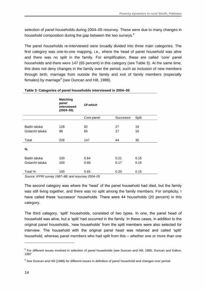
The panel households re-interviewed were broadly divided into three main categories. The
first category was one-to-one mapping, i.e., where the head of panel household was alive
and there was no spilt in the family. For simplification, these are called ‘core’ panel
households and there were 147 (65 percent) in this category (see Table 3). At the same time,
this does not deny changes in the family over the period, such as inclusion of new members
through birth, marriage from outside the family and exit of family members (especially
females) by marriage9 (see Duncan and Hill, 1988).
Table 3: Categories of panel households interviewed in 2004–05
Matching panel interviewed (2004–05)
Of which
Core panel Successor Split
Badin taluka 128 82 27 19
Golarchi taluka 98 65 17 16
Total 226 147 44 35
%
Badin taluka 100 0.64 0.21 0.15
Golarchi taluka 100 0.66 0.17 0.16
Total % 100 0.65 0.20 0.15
Source: IFPRI survey 1987–88; and resurvey 2004–05
The second category was where the ‘head’ of the panel household had died, but the family
was still living together, and there was no split among the family members. For simplicity, I
have called these ‘successor’ households. There were 44 households (20 percent) in this
category.
The third category, ‘split’ households, consisted of two types. In one, the panel head of
household was alive, but a ‘split’ had occurred in the family. In these cases, in addition to the
original panel households, ‘new households’ from the split members were also selected for
interview. The household with the original panel head was retained and called ‘split’
household, whereas panel members who had split from this – whether one or more than one
8 For different issues involved in selection of panel households (see Duncan and Hill, 1985; Duncan and Kalton,
1987
9 See Duncan and Hill (1988) for different issues in definition of panel household and changes over period.
Poverty dynamics in rural Sindh, Pakistan
15
– were treated as ‘new panel households’. The second type of household in the ‘split’
category were those where the ‘original head of panel household’ had died, and his family
had also ‘split’ into ‘new households’. There were a total of 35 ‘split’ households (15 percent)
in the resurvey.
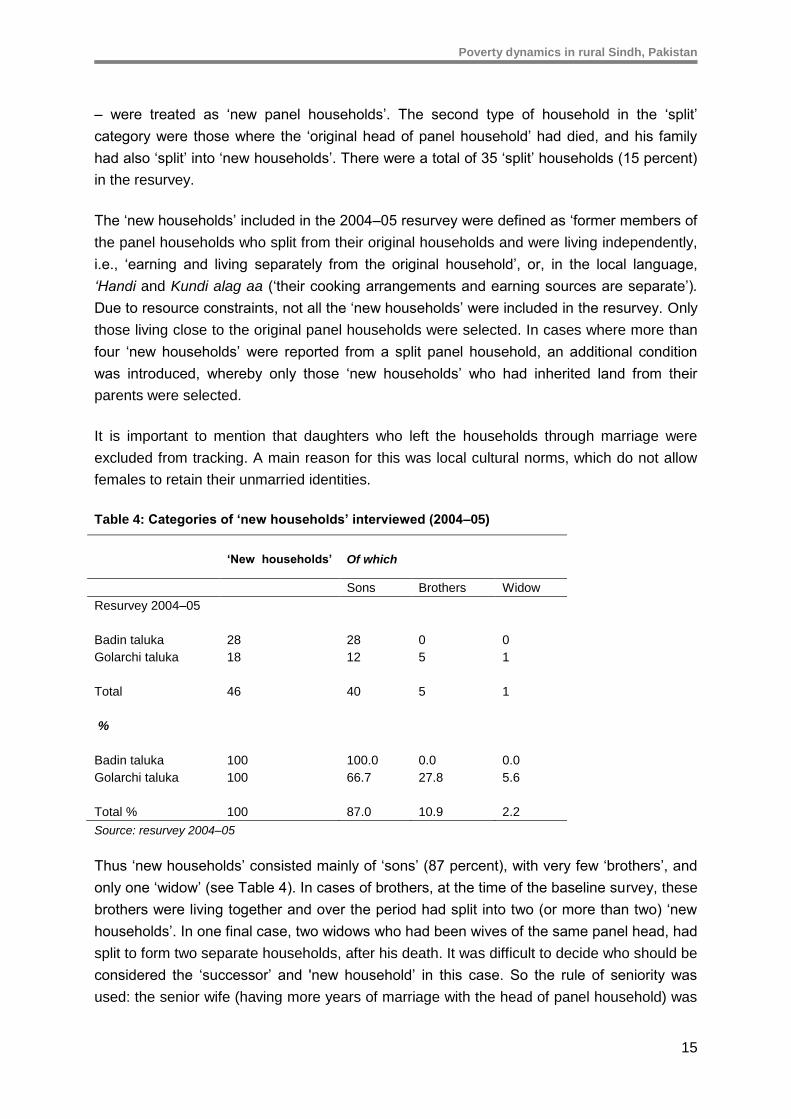
The ‘new households’ included in the 2004–05 resurvey were defined as ‘former members of
the panel households who split from their original households and were living independently,
i.e., ‘earning and living separately from the original household’, or, in the local language,
‘Handi and Kundi alag aa (‘their cooking arrangements and earning sources are separate’).
Due to resource constraints, not all the ‘new households’ were included in the resurvey. Only
those living close to the original panel households were selected. In cases where more than
four ‘new households’ were reported from a split panel household, an additional condition
was introduced, whereby only those ‘new households’ who had inherited land from their
parents were selected.
It is important to mention that daughters who left the households through marriage were
excluded from tracking. A main reason for this was local cultural norms, which do not allow
females to retain their unmarried identities.
Table 4: Categories of ‘new households’ interviewed (2004–05)
‘New households’ Of which
Sons Brothers Widow
Resurvey 2004–05
Badin taluka 28 28 0 0
Golarchi taluka 18 12 5 1
Total 46 40 5 1
%
Badin taluka 100 100.0 0.0 0.0
Golarchi taluka 100 66.7 27.8 5.6
Total % 100 87.0 10.9 2.2
Source: resurvey 2004–05
Thus ‘new households’ consisted mainly of ‘sons’ (87 percent), with very few ‘brothers’, and
only one ‘widow’ (see Table 4). In cases of brothers, at the time of the baseline survey, these
brothers were living together and over the period had split into two (or more than two) ‘new
households’. In one final case, two widows who had been wives of the same panel head, had
split to form two separate households, after his death. It was difficult to decide who should be
considered the ‘successor’ and 'new household’ in this case. So the rule of seniority was
used: the senior wife (having more years of marriage with the head of panel household) was
Poverty dynamics in rural Sindh, Pakistan
16
considered as the ‘successor’ and the other widow as a ‘new household’. There was only
one such household in the whole resurvey.
4 Sampling attrition
One issue that arises in the longitudinal survey is sample attrition. Attrition is likely to be
selective in terms of characteristics and key economic and social variables, such as
schooling, income or assets. In the case of high attrition, the averages for number of
outcome variables can differ significantly between those who are lost in the resurvey (not re-
interviewed) and those who are traced and re-interviewed. Thus, high attrition is likely to
produce biased statistical and econometrical estimates based on longitudinal data. Such
attrition may be particularly severe in rural areas of developing counties, where mobility is
considered very high due to migration between rural and urban areas (see Alderman, et al.,
2001; Leon and Dercon, 2008).
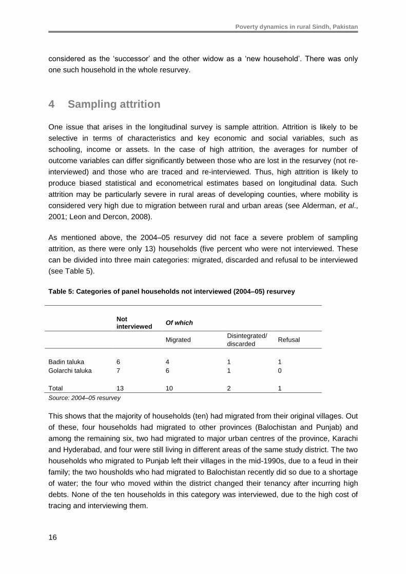
As mentioned above, the 2004–05 resurvey did not face a severe problem of sampling
attrition, as there were only 13) households (five percent who were not interviewed. These
can be divided into three main categories: migrated, discarded and refusal to be interviewed
(see Table 5).
Table 5: Categories of panel households not interviewed (2004–05) resurvey
Not interviewed
Of which
Migrated
Disintegrated/
discarded Refusal
Badin taluka 6 4 1 1
Golarchi taluka 7 6 1 0
Total 13 10 2 1
Source: 2004–05 resurvey
This shows that the majority of households (ten) had migrated from their original villages. Out
of these, four households had migrated to other provinces (Balochistan and Punjab) and
among the remaining six, two had migrated to major urban centres of the province, Karachi
and Hyderabad, and four were still living in different areas of the same study district. The two
households who migrated to Punjab left their villages in the mid-1990s, due to a feud in their
family; the two housholds who had migrated to Balochistan recently did so due to a shortage
of water; the four who moved within the district changed their tenancy after incurring high
debts. None of the ten households in this category was interviewed, due to the high cost of
tracing and interviewing them.
Poverty dynamics in rural Sindh, Pakistan
17
The second category among the non-interviewed was those who no longer exist; for
simplicity, we call them ‘disintegrated households’. One head of household and spouse had
died a long time previously, and in the other, the male head of household died and his widow
left the study area. In the last dropout category, the head of panel household had died and
his eldest son – who became the head of household – refused to grant an interview. The
research team respected his right of refusal.10
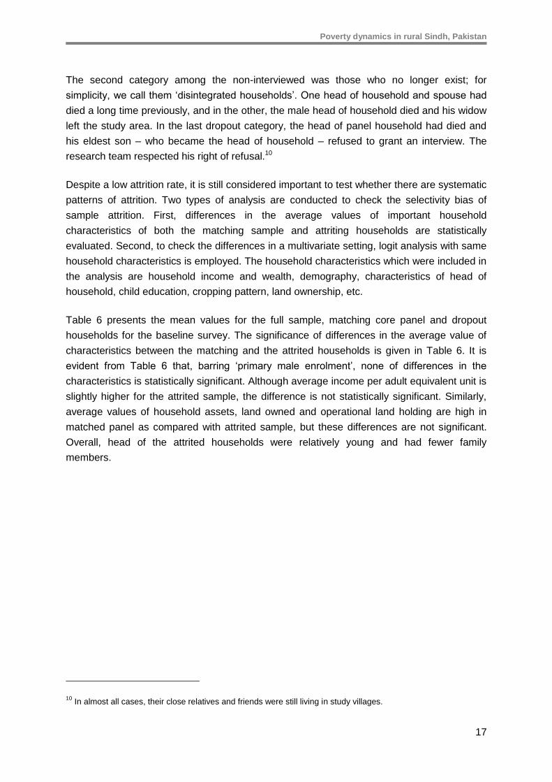
Despite a low attrition rate, it is still considered important to test whether there are systematic
patterns of attrition. Two types of analysis are conducted to check the selectivity bias of
sample attrition. First, differences in the average values of important household
characteristics of both the matching sample and attriting households are statistically
evaluated. Second, to check the differences in a multivariate setting, logit analysis with same
household characteristics is employed. The household characteristics which were included in
the analysis are household income and wealth, demography, characteristics of head of
household, child education, cropping pattern, land ownership, etc.
Table 6 presents the mean values for the full sample, matching core panel and dropout
households for the baseline survey. The significance of differences in the average value of
characteristics between the matching and the attrited households is given in Table 6. It is
evident from Table 6 that, barring ‘primary male enrolment’, none of differences in the
characteristics is statistically significant. Although average income per adult equivalent unit is
slightly higher for the attrited sample, the difference is not statistically significant. Similarly,
average values of household assets, land owned and operational land holding are high in
matched panel as compared with attrited sample, but these differences are not significant.
Overall, head of the attrited households were relatively young and had fewer family
members.
10 In almost all cases, their close relatives and friends were still living in study villages.
Poverty dynamics in rural Sindh, Pakistan
18
Table 6: Significance of difference for mean values for matching panel and attrited households (1987–88 – 2004–05)
Full panel 1987–88 Matching panel Attriting Difference
Sample size Households (239 ) Households (225 ) Households (14 ) Mean [matching and attriting sample]
Mean Std. dev. Mean Std. dev. Mean Std. dev. Difference
Income per adult equivalent (AEUI) 331.18 297.04 329.25 299.30 362.06 265.93 -32.80
Family size 9.26 4.63 9.38 4.68 7.43 3.32 1.95
Dependency ratio 1.22 0.85 1.20 0.84 1.43 0.97 -0.23
Age household head 42.49 13.49 42.74 13.76 38.50 7.19 4.24
Head primary education 42.49 13.49 0.19 0.39 0.07 0.27 0.12
Head secondary education 0.18 0.39 0.07 0.25 0.14 0.36 -0.08
Occupation agriculture 0.07 0.26 0.87 0.34 0.86 0.36 0.01
Primary enrolment (male) 21.09 39.77 22.19 40.62 3.57 13.36 18.61*
Primary enrolment (female) 4.88 20.88 5.19 21.48 0.00 0.00 5.19
Secondary enrolment (male) 14.09 33.81 14.30 34.13 10.71 28.95 3.58
Secondary enrolment (female) 12.59 30.23 12.70 30.37 10.71 28.95 1.99
Owned land (acre/household) 13.10 23.02 13.33 23.57 9.39 10.71 3.94
Average value of household assets (Rs) 19,942 49,662 20,253 51,037 14,948 15,520 5,304
Non-farm income (%) 28.95 34.22 28.75 34.36 32.14 32.99 -3.39
Agriculture wages (%) 5.10 12.12 5.22 12.43 3.14 4.52 5.22
Livestock dairy income (%) 5.87 13.27 6.09 13.58 2.27 5.60 6.09
Sugarcane grower 0.18 0.38 0.18 0.38 0.21 0.43 -0.04
Operated land (acres/household) 10.81 12.04 10.90 12.26 9.32 7.62 1.58
Net sown area (Rabi) 3.03 4.66 3.02 4.69 3.14 4.36 -0.12
Net sown area (Kharif)) 9.01 8.81 9.07 8.94 8.07 6.65 1.00
Statistically significant according to t-value (two-tailed significance) and assuming equal variable in both groups. *Significance atten percent; **Significance at five percent ; ***Significance at one percent.
Sources: IFPRI survey 1987–88 and 2004–05 resurvey; one panel household was dropped from 2004–05 resurvey due to incomplete information, so the
number of attrited households became 14.
Poverty Dynamics in Rural Sindh, Pakistan
19
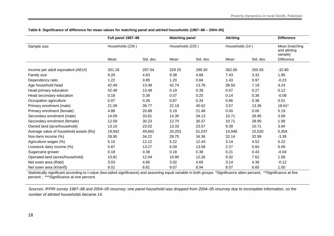
Given the skewed distribution of sample into matched and attrited, logit specification is
preferred over the probit model. Table 7 presents the results of logit estimates. Evidently,
none of the characteristics turns out to be statistically significant. In terms of goodness of fit,
the selected specification predicts 94 percent of cases correctly with a significant likelihood
ratio. Nonetheless, the pseudo R-squared is quite low. As the number of observations in one
group is very small, results should be interpreted accordingly. Table 7. Logit estimates
[matching panel (225) =1, attriting households (14) =0]
Table 7: Logit estimates [matching panel (225) =1, attriting households (14) =0]
Coefficient Significance
Income per adult equivalent (AEUI) 0.000 0.896
Family size 0.084 0.468
Dependency ratio -0.196 0.621
Age household head 0.034 0.251
Head primary education 0.617 0.608
Head secondary education -0.55 0.599
Occupation agriculture 0.896 0.402
Primary enrolment (male) 0.412 0.995
Primary enrolment (female) -0.014 0.415
Secondary enrolment (male) 0.001 0.932
Secondary enrolment (female) 0.195 0.999
Owned land (acre/household) 0.018 0.605
Average value of household assets (Rs) 0.000 0.976
Non-farm income (%) 0.013 0.263
Agriculture wages 0.032 0.559
Livestock 0.159 0.152
Sugarcane grower -0.484 0.562
Operated land (acres/household) -0.007 0.883
Net sown area(Rabi) -0.025 0.808
Net sown area(Kharif)) 0.019 0.776
Badin taluka 1.163 0.11
Intercept -1.435 0.466
Model Summary
Percentage correctly
predicted
Log likelihood Cox and Snell
R-squared
Pseudo R-squared
94.1 82.518 0.100 0.277
After establishing that there was no attrition bias in the 2004–05 resurvey, the next section
analyses the poverty transitions among the panel matching households over the period of the
two surveys.
Poverty Dynamics in Rural Sindh, Pakistan
20
Poverty Dynamics in Rural Sindh, Pakistan
21
5 Poverty dynamics
This section estimates and compares poverty incidence for 1987–88 and 2004–05 for
matching panel sample. In addition, this section also examines the nature and dynamics of
poverty and key factors associated with different poverty status.
Choice of welfare dynamics
This study adopts income as a welfare measure for poverty analysis. There are three main
reasons for this. Firstly, in the baseline survey (1986–87 to 1990–91), income data was
collected in the various rounds and in great detail in different components. Alderman and
Garcia (1993) argue that income data collected in various rounds and components, like the
IFPRI study, has fewer chances of fluctuations than data usually collected in single-shot
interviews in cross-section surveys. Secondly, income and its sources have been a main
focus for evaluating economic welfare and poverty analysis for many studies based on the
IFPRI baseline data set (see Alderman and Garcia, 1993; Adams and He, 1995; Baulch and
McCulloch, 1998, 2002). This provides an incentive and opportunity to compare changes in
poverty incidence, based on the same welfare indicator, with the early studies on the IFPRI
baseline survey. Thirdly, it is also argued that looking at income and its different sources
provides rich insights to help improve our understanding of the poverty dynamics and
livelihoods of poor people (Fields et. al., 2003; McKay, 2000; Ellis, 1998; 2000). At the same
time, it is also important to note that Deaton (1997) and Ravallion (1993) argue that
expenditures are a better welfare measure than income.
Income measurement and comparison
There are a number of issues and challenges involved in measuring and comparing
household income data. These range from the definition of the household, to different
components of income, their valuation, and consumption. In comparing two data sets,
especially panel data, an additional and legitimate concern relates to consistency of
definitions and estimates of key variables, such as sources of income, recall period, price
indices, and year of comparison between the two surveys. There are no hard and fast rules
for classifying and decomposing income into different sources. It depends mainly on the
purpose of the analysis, the availability of suitable methods, and data constraints (see
Deaton, 1995; Gaiha, 1988; Sundrum, 1990). Following the methodology used by Alderman
and Garcia (1993) and Adams and Jane (1995), household income was estimated from six
main sources: net crop profit, farm wages, livestock income, non-farm, rental, and income
from transfers. To maintain consistency and comparability with the baseline survey, the
analysis has tried to strictly follow the income definitions used in the baseline data.
Poverty Dynamics in Rural Sindh, Pakistan
22
Where it was not possible to follow the baseline definition, the same definition was used for
both the surveys (see Appendix 2 for methodology used for constructing income
aggregates).
Updating and adopting a poverty line
It is not easy to obtain a reasonable poverty line for inter-temporal comparisons of poverty,
and in the case of Pakistan it becomes an even more difficult task. A main reason for this lies
in the difficulty of obtaining a reasonable and representative price index for the two periods
(in the absence of very low coverage of rural prices in the general price deflator available at
the whole country level). Secondly, it was only in 2002 that an official poverty line was
adopted at country level.11 One simple and straightforward way to address this is to use the
official available poverty line – Rs.878.64 per capita per month – for 2004–05, and then
deflate it to the baseline year. Unfortunately, there are some potential pitfalls in using this for
the present analysis.
The official poverty line is available only at country level, and is not separately available for
rural areas of the country. To adopt this for the present analysis, it would have to be deflated
by using the consumer price index (CPI) deflator to the baseline period, 1987–88. However,
very serious concerns are raised about the use of CPI for poverty analysis in Pakistan (see
Jamal, 2007; WB, 2002; 2007). In the light of these, it appeared more appropriate to use the
poverty lines estimated by Jamal (2002, 2007), for three reasons.
Firstly, poverty lines are available for the both the required survey years, 1987–88 and 2004–
05, so I do not need to inflate or deflate this. Secondly, this poverty line is available
separately for rural areas of the country. It therefore represents the changes in price indices
better than the single poverty line available for the whole country. Thirdly, the poverty
estimates are based on the widely used data set for poverty analysis, Pakistan Integrated
Household Survey/Household Integrated Economic Surveys (PIHS/HIES) from 1987–88 to
2004–05. The caloric cut-off point used for the estimation was 2,550 calories per adult per
day for rural areas. The caloric requirement for the bottom quintile is kept constant in the
estimations of the successive poverty lines for the two survey years, 1987–88 to 2004–05.
Despite the suitability of the poverty line used for the present analysis, it is important to note
that the basket of goods and consumption patterns of households may have changed over
the period.12
11 See Jafri (2002) for different issues involved in setting the official poverty line in Pakistan.
12 For a detailed discussion on issues involved in comparison of poverty for two periods and its limitations, see
Deaton (1995), Thorbecke (2003), and McKay (2007).
Poverty Dynamics in Rural Sindh, Pakistan
23
The poverty line adopted for the present analysis is an absolute poverty line of Rs.225 per
capita per month for the baseline survey, 1987–88; and Rs.778 per capita per month for the
2004–05 resurvey13.
Poverty Indices
The poverty indices used in the analysis are those of Foster, Greer and Thorbecke (1984),
and are given by
Pα = n
1
]/[ zyizpyi
α
In this yi is the real per capita household income, n is total household population, z is the
poverty line, and α the degree of aversion to inequality among the poor. If α =0, P 0 is the
headcount measure of the proportion of population whose per capita monthly income falls
below the poverty. If α =1, P is the poverty gap ratio which considers depth of poverty. This
indicates the average shortfall of income from the poverty line and informs the required per
capita contribution to lift poor people out of poverty. If α =2, P is the squared poverty gap
ratio which shows the severity of poverty. This is more sensitive to income distribution among
poor people and captures the degree of inequality among poor people. I have used
household size as weights in poverty calculations to correct possible bias associated with
household size.
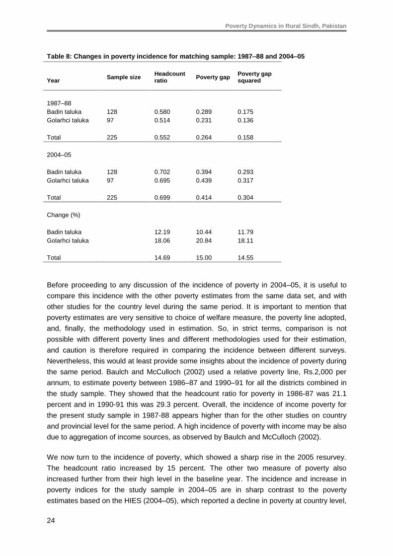
5.1 Changes in poverty between 1987-88 and 2004-5
Aggregate measures of poverty based on the absolute poverty line for the matching panel
sample only are presented in Table 8. The headcount measure of poverty shows that over
half of the sample population (55 percent) was poor in 1987–88. The other two poverty
measures, mean distance from the poverty line, and severity of poverty, were also very high
in the baseline period.
13 Incidentally, it turns out that the poverty line adopted is almost the same, if I use average agricultural GDP
deflator, which was 3.5 over the 1987–88 to 2004–05 period. On the one hand, if I multiply the baseline poverty line, 1987–88, Rs. 225, with the agricultural GDP deflator (3.5), it turns out as Rs. 787.5, for 2004–05: a difference of only ten rupees from the poverty line adopted for 2004–05. On the other hand, if we divide the current poverty line, 2004–05, Rs.778, with the GDP deflator (3.5), to get the baseline poverty line, 1987–88, it turns out to be Rs. 222.3: a difference of only Rs. 2.7. So, overall, the chosen poverty line of Rs. 225 maintains consistency in comparisons between the two surveys.
Poverty Dynamics in Rural Sindh, Pakistan
24
Table 8: Changes in poverty incidence for matching sample: 1987–88 and 2004–05
Year Sample size
Headcount ratio
Poverty gap Poverty gap squared
1987–88
Badin taluka 128 0.580 0.289 0.175
Golarhci taluka 97 0.514 0.231 0.136
Total 225 0.552 0.264 0.158
2004–05
Badin taluka 128 0.702 0.394 0.293
Golarhci taluka 97 0.695 0.439 0.317
Total 225 0.699 0.414 0.304
Change (%)
Badin taluka 12.19 10.44 11.79
Golarhci taluka 18.06 20.84 18.11
Total 14.69 15.00 14.55
Before proceeding to any discussion of the incidence of poverty in 2004–05, it is useful to
compare this incidence with the other poverty estimates from the same data set, and with
other studies for the country level during the same period. It is important to mention that
poverty estimates are very sensitive to choice of welfare measure, the poverty line adopted,
and, finally, the methodology used in estimation. So, in strict terms, comparison is not
possible with different poverty lines and different methodologies used for their estimation,
and caution is therefore required in comparing the incidence between different surveys.
Nevertheless, this would at least provide some insights about the incidence of poverty during
the same period. Baulch and McCulloch (2002) used a relative poverty line, Rs.2,000 per
annum, to estimate poverty between 1986–87 and 1990–91 for all the districts combined in
the study sample. They showed that the headcount ratio for poverty in 1986-87 was 21.1
percent and in 1990-91 this was 29.3 percent. Overall, the incidence of income poverty for
the present study sample in 1987-88 appears higher than for the other studies on country
and provincial level for the same period. A high incidence of poverty with income may be also
due to aggregation of income sources, as observed by Baulch and McCulloch (2002).
We now turn to the incidence of poverty, which showed a sharp rise in the 2005 resurvey.
The headcount ratio increased by 15 percent. The other two measure of poverty also
increased further from their high level in the baseline year. The incidence and increase in
poverty indices for the study sample in 2004–05 are in sharp contrast to the poverty
estimates based on the HIES (2004–05), which reported a decline in poverty at country level,
Poverty Dynamics in Rural Sindh, Pakistan
25
as discussed in Section 2. However, for the purpose of the present analysis, it would be
more useful to compare the 2004–05 resurvey findings with other micro-level studies in the
country. For instance, the World Bank (2002) reports the poverty incidence for the panel
households for the Badin district to be 67 percent. This was the highest for any irrigated area
in the study. Similarly, Hussain (2003), based on a primary survey in the eight poorest
districts in the country, including Badin district, reports an 85 percent incidence of poverty for
Badin. It appears plausible that with increased number of water-related shocks and without
any visible improvement in rural infrastructure or event of a good fortune in the study areas,
the incidence of poverty may have further deteriorated between the two surveys.
Moreover, the sharp increase in poverty for the study sample also appears to be in line with
the main observation of the Oxford Policy Management (OPM) (2003) report. This report
argues that the country faced serious drought and water shortage 1998–99 and 2001–02,
and its agricultural growth was severely affected by this, as discussed in Section 2. The
increase in rural poverty in Pakistan was mainly attributed to this. The report cites Sindh and
Baluchistan as the provinces worst affected by drought, and in these provinces the incidence
of poverty also increased more sharply than in other parts of the country.
5.2 Change in poverty for agrarian groups
For policy purposes it is useful and informative to know the incidence and transition of
poverty among different agricultural occupational groups, as this improves the potential of
targeting poor households. This section presents the incidence and severity of poverty
among the different agricultural groups in the study sample. These groups are defined as:
landless labourers, who neither own land nor rent land; tenants, who do not own land but
who rent land on a sharecropping basis from land owners; owner tenants, who combine their
own land with renting land; and land owners – who own land but do not rent land on fixed or
sharing contracts. The incidence and severity of poverty for different agrarian groups is
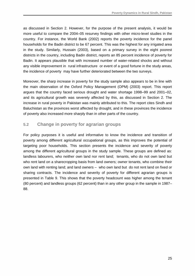
presented in Table 9. This shows that the poverty headcount was higher among the tenant
(80 percent) and landless groups (62 percent) than in any other group in the sample in 1987–
88.
Poverty Dynamics in Rural Sindh, Pakistan
26
Table 9: Poverty incidence and changes for different tenurial groups (based on income poverty): 1987–88 and 2004–05
Year Sample size Head- count ratio
Poverty gap
Poverty gap squared
1987–88
Landless 14 0.624 0.422 0.327
Tenant 81 0.800 0.402 0.243
Owner tenant 62 0.470 0.219 0.132
Land owner 68 0.370 0.145 0.075
Total 225 0.552 0.264 0.158
2004–05
Landless 27 0.742 0.408 0.301
Tenant 53 0.918 0.590 0.479
Owner tenant 44 0.623 0.398 0.283
Land owner 101 0.626 0.339 0.231
Total 225 0.699 0.414 0.304
Change (%)
Landless 11.848 -1.460 -2.597
Tenant 11.820 18.753 23.593
Owner tenant 15.308 17.907 15.147
Land owner 25.621 19.334 15.587
Total 14.689 15.000 14.553
Definitions: landless: own land=0 and operating land=0; tenant: own=0 and hiring in >0; owner-tenant: Own>0 and hiring in >0; landowner: own>0 and hiring in=0
The estimates for the 2004–05 resurvey also show that poverty deteriorated further among
all the agricultural groups, particularly among tenants. In 2004–05, almost all the tenant
households (92 percent) were living below the poverty level. The severity of poverty also
worsened more for the tenants (23.6 percent) than for any other group in the study sample.
Among the landless households nearly three-quarters were unable to meet the minimum
level of food intake in 2004–05, despite a minor reduction in the poverty gap (-1.5) and in the
severity of poverty (-2.6). This indicates that these two groups, tenants and landless, are very
vulnerable to poverty from a minor shock in their livelihoods.
A main explanation for the sharp increase in poverty for almost all the agrarian groups in the
study sample appears mainly from weather-related shocks in the study sample (such as
cyclones, heavy rains, water shortage and drought) between the two surveys. It was also
mentioned by a number of respondents during 2004–05 resurvey, and in qualitative
interviews, that these shocks adversely affected the quality of land and cropping cultivation in
the study sample.
Poverty Dynamics in Rural Sindh, Pakistan
27
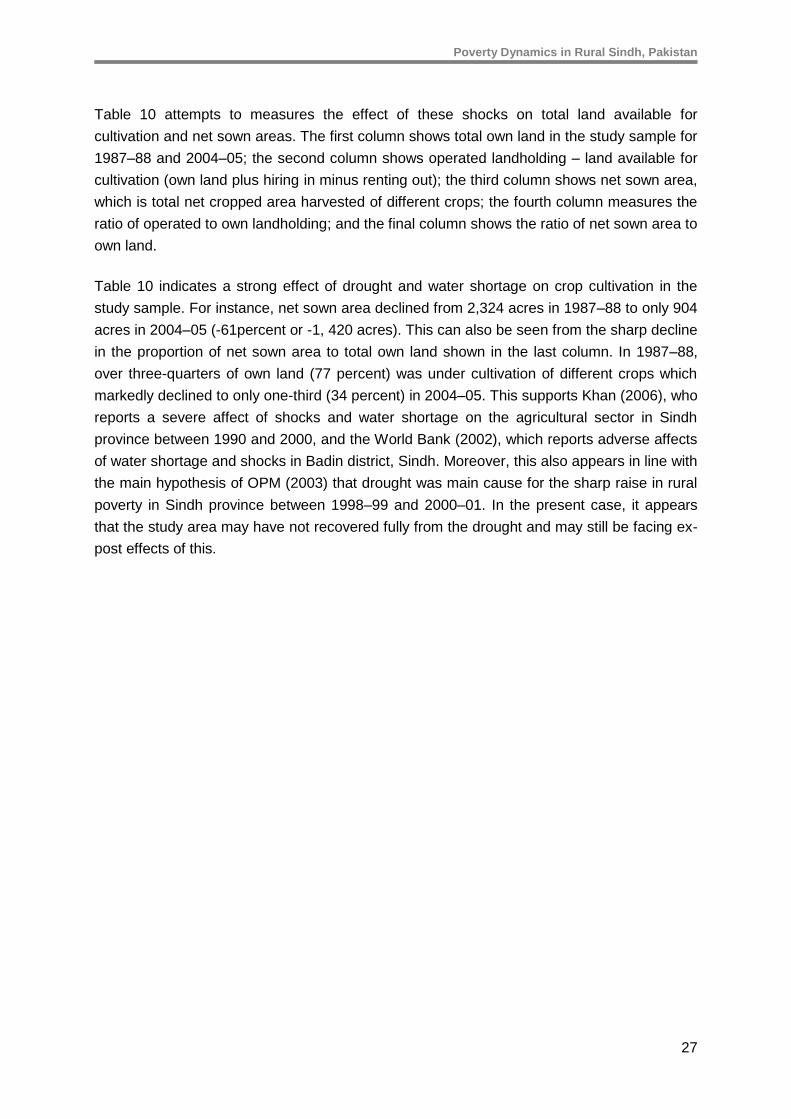
Table 10 attempts to measures the effect of these shocks on total land available for
cultivation and net sown areas. The first column shows total own land in the study sample for
1987–88 and 2004–05; the second column shows operated landholding – land available for
cultivation (own land plus hiring in minus renting out); the third column shows net sown area,
which is total net cropped area harvested of different crops; the fourth column measures the
ratio of operated to own landholding; and the final column shows the ratio of net sown area to
own land.
Table 10 indicates a strong effect of drought and water shortage on crop cultivation in the
study sample. For instance, net sown area declined from 2,324 acres in 1987–88 to only 904
acres in 2004–05 (-61percent or -1, 420 acres). This can also be seen from the sharp decline
in the proportion of net sown area to total own land shown in the last column. In 1987–88,
over three-quarters of own land (77 percent) was under cultivation of different crops which
markedly declined to only one-third (34 percent) in 2004–05. This supports Khan (2006), who
reports a severe affect of shocks and water shortage on the agricultural sector in Sindh
province between 1990 and 2000, and the World Bank (2002), which reports adverse affects
of water shortage and shocks in Badin district, Sindh. Moreover, this also appears in line with
the main hypothesis of OPM (2003) that drought was main cause for the sharp raise in rural
poverty in Sindh province between 1998–99 and 2000–01. In the present case, it appears
that the study area may have not recovered fully from the drought and may still be facing ex-
post effects of this.
Poverty Dynamics in Rural Sindh, Pakistan
28
Table 10: Changes in irrigation and cultivation intensity for panel households: 1987–88 and 2004–05
Own land
(acres)
Land operated
(acres)
Net sown
area
(acres)
Ratio
(operated/own)
Ratio
(net sown/
own land)
(1) (2) (3) (4) (5)
1987–88
Badin taluka 1,457 1,070 1,018 0.73 0.70
Golarhci taluka 1,542 1,383 1,306 0.90 0.85
Total 2,999 2,453 2,324 0.82 0.77
2004–05
Badin taluka 1,042 571 531 0.55 0.51
Golarhci taluka 1,580 662 373 0.42 0.24
Total 2,622 1,232 904 0.47 0.34
Change (absolute)
Badin taluka (-415) (- 499) (-487) (- 0.19) (- 0.19)
Golarhci taluka 38 (- 722) (- 933) (- 0.48) (- 0.61)
Total -( 377) -1,221 (-1,420) (- 0.35) (- 0.43)
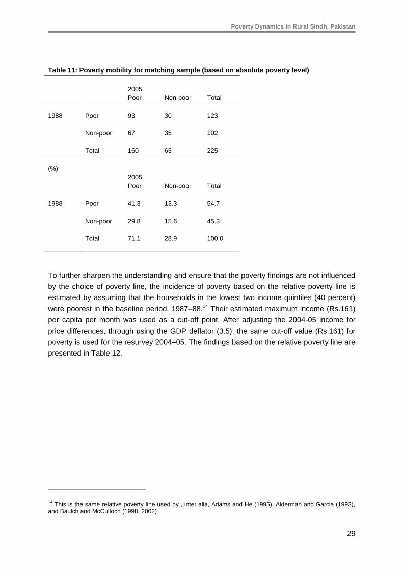
5.3 Poverty Mobility: 1987-88 and 2004-05
Poverty mobility based on absolute poverty (headcount ratio) is shown in the poverty
transition matrices in Table 11. The rows show the poverty incidence in the baseline period,
1987–88, and the columns poverty in the 2005 resurvey. This shows that 41.3 percent of
poor households in 1987–88 remained poor in 2004–05, whereas, only 15.6 percent were
non-poor in both the surveys. The percentage of poor households who moved out of poverty
was only 13.3 percent (30 households), while the percentage of households who entered into
poverty was twice as high, at 29.8 percent (67 households). This indicates that between the
two surveys the probability of entering into poverty was much higher than that of escaping
from it.
Poverty Dynamics in Rural Sindh, Pakistan
29
Table 11: Poverty mobility for matching sample (based on absolute poverty level)
2005
Poor Non-poor Total
1988 Poor 93 30 123
Non-poor 67 35 102
Total 160 65 225
(%)
2005
Poor Non-poor Total
1988 Poor 41.3 13.3 54.7
Non-poor 29.8 15.6 45.3
Total 71.1 28.9 100.0
To further sharpen the understanding and ensure that the poverty findings are not influenced
by the choice of poverty line, the incidence of poverty based on the relative poverty line is
estimated by assuming that the households in the lowest two income quintiles (40 percent)
were poorest in the baseline period, 1987–88.14 Their estimated maximum income (Rs.161)
per capita per month was used as a cut-off point. After adjusting the 2004-05 income for
price differences, through using the GDP deflator (3.5), the same cut-off value (Rs.161) for
poverty is used for the resurvey 2004–05. The findings based on the relative poverty line are
presented in Table 12.
14 This is the same relative poverty line used by , inter alia, Adams and He (1995), Alderman and Garcia (1993),
and Baulch and McCulloch (1998, 2002)
Poverty Dynamics in Rural Sindh, Pakistan
30
Table 12: Poverty mobility (based on relative poverty line)
2005
Poor Non-poor Total
1988 Poor 62 27 89
Non-poor 75 61 136
Total 137 88 225
(%) 2005
Poor Non-poor Total
1988 Poor 27.6 12.0 39.6
Non-poor 33.3 27.1 60.4
Total 60.9 39.1 100.0
Table 12 also shows that the incidence of poverty has increased from 39.6 percent in 1988 to
60.9 percent in 2005. Like mobility measured in absolute terms, a high percentage of
households, 27 percent, remained in poverty for both the surveys. However, a high
percentage of households, 27.1 percent, remained non-poor when measured in relative
poverty. Like absolute poverty, this also shows that a high percentage of households, 33.3
percent, had fallen into poverty, compared to only 12 percent of households who moved out
of poverty between the two surveys. This finding of high chronic poverty over the long
duration of the sample is in contrast to what Baulch and McCulloch (1998 and 2002) found
for short duration of poverty transition.. One reason for the high incidence of chronic poverty
in 2004–05 could be the influence of drought and weather shocks in the study sample. The
above findings for poverty transitions in 2004–05 are in line with Dorosh and Malik (2006)
and the World Bank (2007). These studies show that poor households in the IFPRI panel
districts, including Badin, increased sharply from 33 percent to 64 percent between the
baseline (1986–87 to 1990–91) and 2001–02. Only nine percent of households escaped out
of poverty, while 40 percent fell into poverty. One-quarter of households, 24 percent,
remained ‘chronically poor’, and 26 percent of households remained non-poor in the study
panel.
Poverty Dynamics in Rural Sindh, Pakistan
31
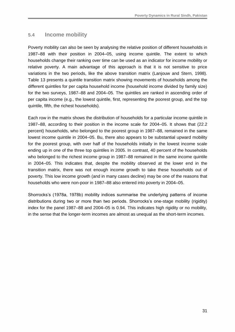
5.4 Income mobility
Poverty mobility can also be seen by analysing the relative position of different households in
1987–88 with their position in 2004–05, using income quintile. The extent to which
households change their ranking over time can be used as an indicator for income mobility or
relative poverty. A main advantage of this approach is that it is not sensitive to price
variations in the two periods, like the above transition matrix (Lanjouw and Stern, 1998).
Table 13 presents a quintile transition matrix showing movements of households among the
different quintiles for per capita household income (household income divided by family size)
for the two surveys, 1987–88 and 2004–05. The quintiles are ranked in ascending order of
per capita income (e.g., the lowest quintile, first, representing the poorest group, and the top
quintile, fifth, the richest households).
Each row in the matrix shows the distribution of households for a particular income quintile in
1987–88, according to their position in the income scale for 2004–05. It shows that (22.2
percent) households, who belonged to the poorest group in 1987–88, remained in the same
lowest income quintile in 2004–05. Bu, there also appears to be substantial upward mobility
for the poorest group, with over half of the households initially in the lowest income scale
ending up in one of the three top quintiles in 2005. In contrast, 40 percent of the households
who belonged to the richest income group in 1987–88 remained in the same income quintile
in 2004–05. This indicates that, despite the mobility observed at the lower end in the
transition matrix, there was not enough income growth to take these households out of
poverty. This low income growth (and in many cases decline) may be one of the reasons that
households who were non-poor in 1987–88 also entered into poverty in 2004–05.
Shorrocks’s (1978a, 1978b) mobility indices summarise the underlying patterns of income
distributions during two or more than two periods. Shorrocks’s one-stage mobility (rigidity)
index for the panel 1987–88 and 2004–05 is 0.94. This indicates high rigidity or no mobility,
in the sense that the longer-term incomes are almost as unequal as the short-term incomes.
Poverty Dynamics in Rural Sindh, Pakistan
32
Table 13: Income mobility: 1987–88 to 2004–05
Quintiles of the 2004–05 per capita income scale
Poorest 2 3 4 Richest
Quintiles of the 1987–88 per capita income scale
Poorest 10 12 11 7 5
2 11 9 10 9 6
3 6 9 12 8 10
4 11 8 9 11 6
Richest 7 7 3 10 18
(%)
Poorest 2 3 4 Richest
Poorest 22.2 26.7 24.4 15.6 11.1
2 24.4 20.0 22.2 20.0 13.3
3 13.3 20.0 26.7 17.8 22.2
4 24.4 17.8 20.0 24.4 13.3
Richest 15.6 15.6 6.7 22.2 40.0
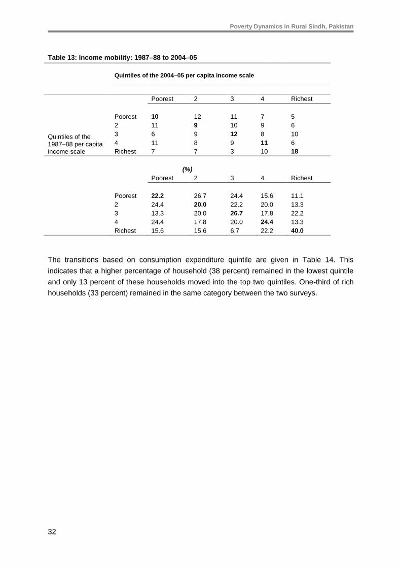
The transitions based on consumption expenditure quintile are given in Table 14. This
indicates that a higher percentage of household (38 percent) remained in the lowest quintile
and only 13 percent of these households moved into the top two quintiles. One-third of rich
households (33 percent) remained in the same category between the two surveys.
Poverty Dynamics in Rural Sindh, Pakistan
33
Table 14: Poverty mobility with (per capita consumption expenditures quintiles)
Quintiles of 2004–05 per capita consumption expenditure scale
2004–05
Lowest 2 3 4 Highest
Lowest 17 11 11 5 1
2 7 8 7 12 11
1987–88 3 9 9 12 9 6
4 8 9 8 8 12
Highest 4 8 7 11 15
(%)
Lowest 2 3 4 Highest
Lowest 37.8 24.4 24.4 11.1 2.2
2 15.6 17.8 15.6 26.7 24.4
3 20.0 20.0 26.7 20.0 13.3
4 17.8 20.0 17.8 17.8 26.7
Highest 8.9 17.8 15.6 24.4 33.3
5.5 Explanation for poverty persistence and poverty transitions
There was a combination of factors which appears relevant to explaining the persistence and
descending of poverty between the two surveys. Following Sen (2003) these poverty groups
are defined as chronically poor (poor remained poor); ascending poor (poor became non-
poor); descending poor (non-poor became poor) and never poor (non-poor remained non-
poor) categories. Table 15 compares changes in demography, human and physical assets,
agriculture, and household income and expenditures for these poverty groups based on
relative poverty. As expected, the category of never poor has the highest mean value for per
adult equivalent income in 2004–05, followed by ascending households, descending
households, and the chronically poor.
Poverty Dynamics in Rural Sindh, Pakistan
34
Table 15: Mean values for key household characteristics according to poverty status: (1987–88 to 2004–05)
Chronically poor
Ascending poor Descending poor
Never poor Total
1988 2005 1988 2005 1988 2005 1988 2005 1988 2005
Average age household head 40.97 53.10 44.52 52.41 42.17 52.43 44.46 51.41 42.74 52.33
Average family size 9.60 9.10 10.63 10.33 8.52 10.12 9.66 10.56 9.38 9.98
Dependency ratio 1.45 0.83 1.44 0.70 1.03 1.06 1.07 1.04 1.20 0.95
Average years of education
Head 0.97 1.79 1.78 3.78 1.55 2.44 2.34 3.44 1.63 2.69
Spouse 0.00 0.00 0.00 0.15 0.13 0.23 0.33 0.66 0.13 0.27
Education
Primary enrolment ten years and above (male) 19.49 25.27 36.42 24.07 14.00 36.22 28.69 27.05 22.19 29.26
Primary enrolment ten years and above (female) 1.61 12.90 6.17 20.37 3.33 13.78 10.66 18.80 5.19 15.69
Primary enrolment (both) 13.92 25.27 32.22 32.10 13.11 36.44 26.50 36.44 19.26 32.84
Secondary enrolment (male) 12.10 16.13 22.22 38.89 8.67 27.20 19.95 43.17 14.30 29.88
Secondary enrolment (female) 0.00 12.90 1.23 18.52 2.67 9.78 4.92 13.39 2.37 12.67
Secondary enrolment (both) 9.68 25.40 20.99 38.46 6.33 27.16 19.95 43.28 12.70 32.40
Literacy, ten years and above (male) 25.31 51.20 59.29 74.50 39.93 57.87 45.51 67.32 39.74 60.59
Literacy, ten years and above (female) 11.29 7.56 15.25 21.17 12.22 10.77 16.46 18.84 13.48 13.32
Literacy, ten years and above (both) 18.17 30.00 35.99 51.20 26.67 35.40 32.27 44.46 26.96 38.26
Assets
Average acres of land owned/hhold 4.40 2.85 5.04 5.72 13.24 10.38 26.19 24.79 13.33 11.65
Asset score 2.65 2.19 3.41 3.78 3.09 2.71 3.75 3.77 3.19 2.98
Asset value (Rs) 7,710 8,865 18,666 21,461 16,320 10,926 38,538 64,589 20,253 26,171
Agriculture
Average acres of land operated/hhold 11.32 4.67 6.74 6.08 11.91 6.16 11.08 5.19 10.90 5.48
Average number of crops cultivated in (Rabi season) 0.77 1.31 0.67 1.52 1.15 1.23 0.97 1.79 0.94 1.44
Average number of crops cultivated in (Kharif season) 1.48 0.92 1.44 1.04 1.59 0.85 1.46 1.15 1.51 0.97
Net sown area (Rabi season) 1.90 2.39 1.50 5.28 4.00 3.30 3.62 3.82 3.02 3.43
Net sown area (Kharif season) 8.07 2.83 6.20 5.19 11.09 2.99 8.89 3.69 9.07 3.40
Rice 0.84 0.52 0.63 0.56 0.65 0.49 0.52 0.36 0.67 0.47
Wheat 0.15 0.15 0.15 0.11 0.19 0.13 0.11 0.08 0.15 0.12
Sunflower (new cash crop) 0.15 0.26 0.23 0.18 0.20
Household expenditures
Average share (%) on food purchase 77.93 66.53 76.54 62.43 74.79 64.69 73.69 58.92 75.57 63.36
Household income
Income per AEU (Rs./nominal) 112.7 301.8 136.7 1319.1 412.2 328.6 532.6 2134.6 329.3 929.7
Income per AEU (Rs. Real) 86.2 376.9 93.9 609.9 265.6
Growth rate (%) -23.5 175.8 -77.2 14.5 -19.3
Poverty Dynamics in Rural Sindh, Pakistan
35
5.5.1 5Key characteristics for chronically poor
The lowest position of the chronically poor is evident in terms of lowest mean value of
income, ownership of land and asset value, average years of head education and literacy
among different age groups in family. Moreover, their vulnerability to shocks in agriculture
also appears higher than other poverty groups. Some important observations are made for
the chronically poor group. Households who remained poor were on average older than other
groups of households. Their mean age value was higher than the average age of head in
2004–05. The average years of education of head and spouse for this group was lower than
average education in 1987–88 and it remained lower after 15 years in the 2004–05 resurvey.
In fact, for both the survey years, no chronically poor spouses had education. Strikingly, this
trend of low education for members of the chronically poor indicates very little improvement
compared with other groups. For instance, primary enrolment for those aged ten years and
above (male and female), secondary enrolment (male and female), and literacy rate (male
and female) for the chronically poor group were lower than the average values in the study
sample. This low improvement is more striking for female members of households. On a
positive note, family members’ achievement in educational indicators in 2004–05 compared
with 1987–88 shows a marked improvement.
Households in chronic poverty had the lowest mean value for land ownership, asset value
(TV, radio, jewellery, etc.) and score in 1987–88 and this remained lower than the average
sample value in 2004–05. The decline in land ownership of 1.4 acres per household (from
4.40 acres in 1987–88 to 2.85 acres in 2004–05) indicates the possibility of some distress
selling between the two surveys. This indicates an increased vulnerability of the chronically
poor group in terms of low assets.
A number of indicators were estimated to capture shocks in agriculture and their effect on
different poverty groups in the study sample. Table 15 shows that average operated land
available for cultivation declined between the two surveys from 10.9 acres to only 5.5 acres
per household. Between the two cropping seasons, the main affected season was Kharif, in
terms of decline in net sown area for cropping. Net own area under different crops in Kharif
declined nearly threefold, from mean value 9.07 acres in 1987–88 to 3.40 acres in 2004–05.
The loss of operated land per household was higher for chronically poor than other
households. They also experienced decline in the number of Kharif crops (from mean value
1.5 to 0.9) and in the main Kharif food crop rice (from 0.85 to 0.52) in 2004–05.
Crop cultivation in the Rabi season experienced a minor improvement, as the mean value
increased for both total net sown area per household (from 3.02 to 3.43 acres) and number
of crops (0.94 to 1.44 acres) between the two surveys. Average cropped area for Rabi food
crop wheat declined (from 0.15 to 0.12). Chronically poor households were the only group of
households who cultivated the same area under wheat in 2004–05 as in 1987–88. This may
indicate a need to maintain security for food. Sunflower emerged as a new cash crop in the
study area in response to water shortage, degrading land quality, and price incentives. The
Poverty Dynamics in Rural Sindh, Pakistan
36
mean value for cultivating sunflower was slightly low for chronically poor households than the
average value for the study sample (0.15 vs. 0.20) in 2004–05.
Households in chronic poverty, on average, were spending a higher share of their income on
food expenditures than the average spending in the study sample in 1987–88 (78 percent vs.
76 percent). In 2004–05 their income share on food expenditures declined slightly compared
with the baseline year; however, this still remained higher in the study sample (67 percent vs.
63 percent). Average per capita income for those in chronic poverty was lowest in 1987–88
(Rs113 vs. Rs.329), and it remained lowest in 2004–05, with further decline (Rs.86 vs.
Rs.266). Overall, the chronically poor experienced) a decline (-24 percent in their income
between the two surveys.
5.5.2 Key characteristics of descending poor
There appears to be a combination of factors to explain the downward mobility for
descending poor households. Firstly, demographic changes in household have been
unfavourable in this category. For instance, descending poor were the group who
experienced the highest increase in family size (from 8.5 to 10.1) between the two surveys.
Secondly, this group was the poverty group who saw the highest depletion of their assets.
Own land, one of the most important assets in a rural economy, declined markedly for the
descending poor, from 13.3 acres in 1987–88 to 10.4 acres in 2004–05. Moreover, this was
the only group of households who also experienced decline in real value of household
assets.
Thirdly, descending poor was the only group which experienced severe shocks in almost all
the estimated indicators in agriculture livelihoods. The decline in number of Kharif crops
(from 1.6 to 0.85) and net sown cropping area (from 11 acres to only three acres) was more
severefor this group than any other group in the same season. Similarly, in Rabi season,
when every other group experienced some improvement in number of crops and net sown
area, the descending poor group experienced decline and stagnation. Its net sown area
declined in Rabi (from 4.0 acres to 3.3 acres) and its overall total number of crop in Rabi
remained stagnant (from 1.2 to 1.2 acres). The cropping area under main Rabi crop, wheat,
declined (from 0.19 to 0.13 acres). Fourthly, the highest decline in income growth –77
percent (from Rs.412 in 1987–88 to only Rs.94 in 2004–05) was in the descending poor
group of households. This indicates that in the study sample the group most affected by
different shocks in agriculture was the descending poor.
5.5.3 Key characters of ascending poor
Table 14 indicates clearly that key characteristics, in terms of education, assets, agriculture,
and change in per capita income for the households who escape from poverty are different
from those which remained poor and entered into poverty. Average years’ education of head
were higher for these households than the overall average for both the survey years. More
Poverty Dynamics in Rural Sindh, Pakistan
37
markedly, the rate of literacy (male and female) and primary and secondary enrolment in
1987–88 was much higher for the escaping poverty category than others in the sample.
Ascending households were the only category who experienced a slight increase in land
ownership and real value of assets over the period. Overall, decline in different indicators of
agriculture was lower than the study sample average for this category. For instance, decline
in operated acres of land for this category was only 0.6 acres, compared with the average
decline of 5.4 acres in the study sample. In terms of change in real adult equivalent income,
escaping poor households experienced a threefold increase in their real income (from Rs.
137 in 1987–88 to Rs.377 in 2004–05), compared with an average decline in income (-19
percent) for the study sample.
5.6 Further insights into poverty transition from qualitative interviews
To further supplement the above analysis, some key findings are reported from the
qualitative interviews with households who were purposively selected according to their
poverty status between the two surveys. In one study village the incidence of poverty
increased over threefold, from 25 percent to 88 percent: four sample households had fallen
into poverty and three households were poor for both the surveys. Four key informant
interviews, two with male heads of household and two with the spouse of each, were
conducted in this village. Both the households were found to be related to each other,
although they were living and earning separately. The main discussion from these detailed
interviews is summarised into three points and set out in Box 1.
The whole village community suffered severely from drought for the five years, 1999 to 2004,
and this severely affected their crop income and also their other sources of income. During
this period, the families survived on the sale of livestock, daily wage income from casual
labour, and local borrowing. The agricultural year 2005 was considered a better crop year
than the previous four years in the study sample.
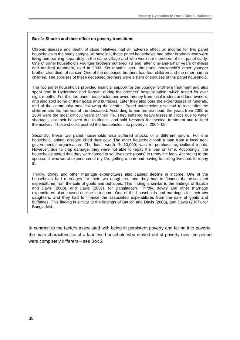
Poverty Dynamics in Rural Sindh, Pakistan
38
Box 1: Shocks and their effect on poverty transitions
Chronic disease and death of close relatives had an adverse effect on income for two panel households in the study sample. At baseline, these panel households had other brothers who were living and earning separately in the same village and who were not members of this panel study. One of panel household’s younger brothers suffered TB and, after one-and-a-half years of illness and medical treatment, died in 2003. Six months later, the panel household’s other younger brother also died, of cancer. One of the deceased brothers had four children and the other had no children. The spouses of these deceased brothers were sisters of spouses of the panel household.
The two panel households provided financial support for the younger brother’s treatment and also spent time in Hyderabad and Karachi during the brothers’ hospitalisation, which lasted for over eight months. For this the panel households borrowed money from local traders and land owners, and also sold some of their goats and buffaloes. Later they also bore the expenditures of funerals, and of the community meal following the deaths. Panel households also had to look after the children and the families of the deceased. According to one female head, the years from 2000 to 2004 were the most difficult years of their life. They suffered heavy losses in crops due to water shortage, lost their beloved due to illness, and sold livestock for medical treatment and to feed themselves. These shocks pushed the households into poverty in 2004–05.
Secondly, these two panel households also suffered shocks of a different nature. For one household, animal disease killed their cow. The other household took a loan from a local non-governmental organisation. The loan, worth Rs.10,000, was to purchase agricultural inputs. However, due to crop damage, they were not able to repay the loan on time. Accordingly, the households stated that they were forced to sell livestock (goats) to repay the loan. According to the spouse, ‘it was worst experience of my life, getting a loan and having to selling livestock to repay it’.
Thirdly, dowry and other marriage expenditures also caused decline in income. One of the households had marriages for their two daughters, and they had to finance the associated expenditures from the sale of goats and buffaloes. This finding is similar to the findings of Baulch and Davis (2008), and Davis (2007), for Bangladesh. Thirdly, dowry and other marriage expenditures also caused decline in income. One of the households had marriages for their two daughters, and they had to finance the associated expenditures from the sale of goats and buffaloes. This finding is similar to the findings of Baulch and Davis (2008), and Davis (2007), for Bangladesh.
In contrast to the factors associated with being in persistent poverty and falling into poverty,
the main characteristics of a landless household who moved out of poverty over the period
were completely different – see Box 2
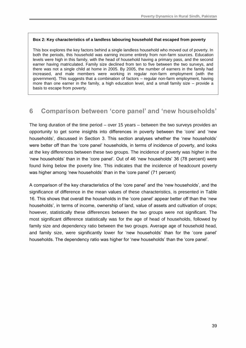
Poverty Dynamics in Rural Sindh, Pakistan
39
Box 2: Key characteristics of a landless labouring household that escaped from poverty
This box explores the key factors behind a single landless household who moved out of poverty. In both the periods, this household was earning income entirely from non-farm sources. Education levels were high in this family, with the head of household having a primary pass, and the second earner having matriculated. Family size declined from ten to five between the two surveys, and there was not a single child at home in 2005. By 2005, the number of earners in the family had increased, and male members were working in regular non-farm employment (with the government). This suggests that a combination of factors – regular non-farm employment, having more than one earner in the family, a high education level, and a small family size – provide a basis to escape from poverty.
6 Comparison between ‘core panel’ and ‘new households’
The long duration of the time period – over 15 years – between the two surveys provides an
opportunity to get some insights into differences in poverty between the ‘core’ and ‘new
households’, discussed in Section 3. This section analyses whether the ‘new households’
were better off than the ‘core panel’ households, in terms of incidence of poverty, and looks
at the key differences between these two groups. The incidence of poverty was higher in the
‘new households’ than in the ‘core panel’. Out of 46 ‘new households’ 36 (78 percent) were
found living below the poverty line. This indicates that the incidence of headcount poverty
was higher among ‘new households’ than in the ‘core panel’ (71 percent)
A comparison of the key characteristics of the ‘core panel’ and the ‘new households’, and the
significance of difference in the mean values of these characteristics, is presented in Table
16. This shows that overall the households in the ‘core panel’ appear better off than the ‘new
households’, in terms of income, ownership of land, value of assets and cultivation of crops;
however, statistically these differences between the two groups were not significant. The
most significant difference statistically was for the age of head of households, followed by
family size and dependency ratio between the two groups. Average age of household head,
and family size, were significantly lower for ‘new households’ than for the ‘core panel’
households. The dependency ratio was higher for ‘new households’ than the ‘core panel’.
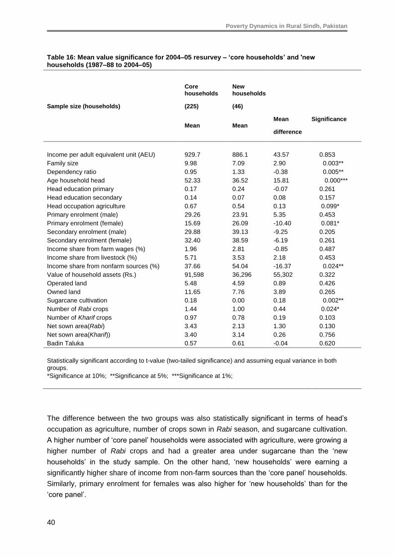
Poverty Dynamics in Rural Sindh, Pakistan
40
Table 16: Mean value significance for 2004–05 resurvey – ‘core households’ and 'new households (1987–88 to 2004–05)
Core households
New households
Sample size (households) (225) (46)
Mean Mean
Mean
difference
Significance
Income per adult equivalent unit (AEU) 929.7 886.1 43.57 0.853
Family size 9.98 7.09 2.90 0.003**
Dependency ratio 0.95 1.33 -0.38 0.005**
Age household head 52.33 36.52 15.81 0.000***
Head education primary 0.17 0.24 -0.07 0.261
Head education secondary 0.14 0.07 0.08 0.157
Head occupation agriculture 0.67 0.54 0.13 0.099*
Primary enrolment (male) 29.26 23.91 5.35 0.453
Primary enrolment (female) 15.69 26.09 -10.40 0.081*
Secondary enrolment (male) 29.88 39.13 -9.25 0.205
Secondary enrolment (female) 32.40 38.59 -6.19 0.261
Income share from farm wages (%) 1.96 2.81 -0.85 0.487
Income share from livestock (%) 5.71 3.53 2.18 0.453
Income share from nonfarm sources (%) 37.66 54.04 -16.37 0.024**
Value of household assets (Rs.) 91,598 36,296 55,302 0.322
Operated land 5.48 4.59 0.89 0.426
Owned land 11.65 7.76 3.89 0.265
Sugarcane cultivation 0.18 0.00 0.18 0.002**
Number of Rabi crops 1.44 1.00 0.44 0.024*
Number of Kharif crops 0.97 0.78 0.19 0.103
Net sown area(Rabi) 3.43 2.13 1.30 0.130
Net sown area(Kharif)) 3.40 3.14 0.26 0.756
Badin Taluka 0.57 0.61 -0.04 0.620
Statistically significant according to t-value (two-tailed significance) and assuming equal variance in both groups.
*Significance at 10%; **Significance at 5%; ***Significance at 1%;
The difference between the two groups was also statistically significant in terms of head’s
occupation as agriculture, number of crops sown in Rabi season, and sugarcane cultivation.
A higher number of ‘core panel’ households were associated with agriculture, were growing a
higher number of Rabi crops and had a greater area under sugarcane than the ‘new
households’ in the study sample. On the other hand, ‘new households’ were earning a
significantly higher share of income from non-farm sources than the ‘core panel’ households.
Similarly, primary enrolment for females was also higher for ‘new households’ than for the
‘core panel’.
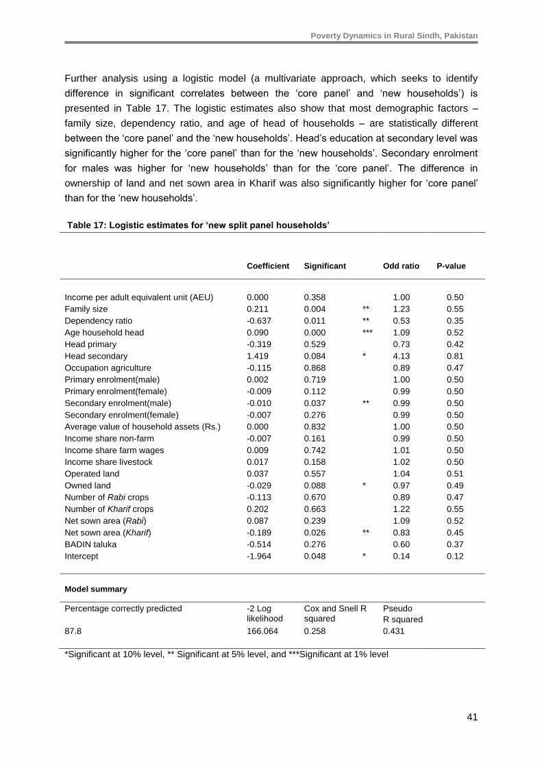
Poverty Dynamics in Rural Sindh, Pakistan
41
Further analysis using a logistic model (a multivariate approach, which seeks to identify
difference in significant correlates between the ‘core panel’ and ‘new households’) is
presented in Table 17. The logistic estimates also show that most demographic factors –
family size, dependency ratio, and age of head of households – are statistically different
between the ‘core panel’ and the ‘new households’. Head’s education at secondary level was
significantly higher for the ‘core panel’ than for the ‘new households’. Secondary enrolment
for males was higher for ‘new households’ than for the ‘core panel’. The difference in
ownership of land and net sown area in Kharif was also significantly higher for ‘core panel’
than for the ‘new households’.
Table 17: Logistic estimates for ‘new split panel households’
Coefficient Significant Odd ratio P-value
Income per adult equivalent unit (AEU) 0.000 0.358 1.00 0.50
Family size 0.211 0.004 ** 1.23 0.55
Dependency ratio -0.637 0.011 ** 0.53 0.35
Age household head 0.090 0.000 *** 1.09 0.52
Head primary -0.319 0.529 0.73 0.42
Head secondary 1.419 0.084 * 4.13 0.81
Occupation agriculture -0.115 0.868 0.89 0.47
Primary enrolment(male) 0.002 0.719 1.00 0.50
Primary enrolment(female) -0.009 0.112 0.99 0.50
Secondary enrolment(male) -0.010 0.037 ** 0.99 0.50
Secondary enrolment(female) -0.007 0.276 0.99 0.50
Average value of household assets (Rs.) 0.000 0.832 1.00 0.50
Income share non-farm -0.007 0.161 0.99 0.50
Income share farm wages 0.009 0.742 1.01 0.50
Income share livestock 0.017 0.158 1.02 0.50
Operated land 0.037 0.557 1.04 0.51
Owned land -0.029 0.088 * 0.97 0.49
Number of Rabi crops -0.113 0.670 0.89 0.47
Number of Kharif crops 0.202 0.663 1.22 0.55
Net sown area (Rabi) 0.087 0.239 1.09 0.52
Net sown area (Kharif) -0.189 0.026 ** 0.83 0.45
BADIN taluka -0.514 0.276 0.60 0.37
Intercept -1.964 0.048 * 0.14 0.12
Model summary
Percentage correctly predicted -2 Log likelihood
Cox and Snell R squared
Pseudo
R squared
87.8 166.064 0.258 0.431
*Significant at 10% level, ** Significant at 5% level, and ***Significant at 1% level
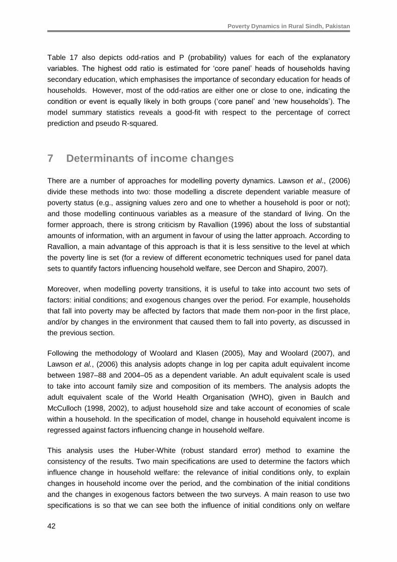
Poverty Dynamics in Rural Sindh, Pakistan
42
Table 17 also depicts odd-ratios and P (probability) values for each of the explanatory
variables. The highest odd ratio is estimated for ‘core panel’ heads of households having
secondary education, which emphasises the importance of secondary education for heads of
households. However, most of the odd-ratios are either one or close to one, indicating the
condition or event is equally likely in both groups (‘core panel’ and ‘new households’). The
model summary statistics reveals a good-fit with respect to the percentage of correct
prediction and pseudo R-squared.
7 Determinants of income changes
There are a number of approaches for modelling poverty dynamics. Lawson et al., (2006)
divide these methods into two: those modelling a discrete dependent variable measure of
poverty status (e.g., assigning values zero and one to whether a household is poor or not);
and those modelling continuous variables as a measure of the standard of living. On the
former approach, there is strong criticism by Ravallion (1996) about the loss of substantial
amounts of information, with an argument in favour of using the latter approach. According to
Ravallion, a main advantage of this approach is that it is less sensitive to the level at which
the poverty line is set (for a review of different econometric techniques used for panel data
sets to quantify factors influencing household welfare, see Dercon and Shapiro, 2007).
Moreover, when modelling poverty transitions, it is useful to take into account two sets of
factors: initial conditions; and exogenous changes over the period. For example, households
that fall into poverty may be affected by factors that made them non-poor in the first place,
and/or by changes in the environment that caused them to fall into poverty, as discussed in
the previous section.
Following the methodology of Woolard and Klasen (2005), May and Woolard (2007), and
Lawson et al., (2006) this analysis adopts change in log per capita adult equivalent income
between 1987–88 and 2004–05 as a dependent variable. An adult equivalent scale is used
to take into account family size and composition of its members. The analysis adopts the
adult equivalent scale of the World Health Organisation (WHO), given in Baulch and
McCulloch (1998, 2002), to adjust household size and take account of economies of scale
within a household. In the specification of model, change in household equivalent income is
regressed against factors influencing change in household welfare.
This analysis uses the Huber-White (robust standard error) method to examine the
consistency of the results. Two main specifications are used to determine the factors which
influence change in household welfare: the relevance of initial conditions only, to explain
changes in household income over the period, and the combination of the initial conditions
and the changes in exogenous factors between the two surveys. A main reason to use two
specifications is so that we can see both the influence of initial conditions only on welfare
Poverty Dynamics in Rural Sindh, Pakistan
43
changes, and also a combination of change variables over the period. The specific variables
considered as potential factors for poverty transitions were divided into the following
categories: firstly, demographic changes (family size, dependency ratio and age of
household head); secondly, human development (primary and secondary enrolment, children
out of school, and literacy among the family members); thirdly, asset ownership (owned land
and asset score15), fourthly, different income sources, household members working in non-
farm employment, and finally, changes in household agriculture (number of total crops
cultivated and total area under different crops in the two seasons). The change variables
were calculated by subtracting the base year, 1988 values from the 2004–05 resurvey values
(see Jamal and Lohano (2008) for preliminary findings)16. Due to over 15 years’ gap in the
two surveys and induced changes over the period, the problem of endogeneity may exist in
these models.
7.1 Main findings and explanation
It is important to note that change in log of real income per adult equivalent unit declined
between the two surveys. A summary of means and standard deviations of the explanatory
variables is given in Appendix 1. Simple regression results are given in Table 18 and Table
19. Both the models indicate a good fit, as measured by its adjusted R-squared – which is
above 0.54. F-value is also significant at one percent level. The last column in each model
reports t-value, re-estimated to allow for heteroscedasticity in the model specification. All
results with the robust standard error method remain significant as estimated with simple
regression method. Multicolinearity among the independent variables makes some
coefficients statistically less efficient and insignificant. This was tested with variance inflation
factors (VIF). Individual VIF greater than ten and mean values substantially higher than one
indicates multicolinearity, and points to less reliability about the magnitude of the coefficients
(Wooldridge, 2006). None of the individual factors’ value was higher than four and the mean
VIF value ranged between 1.50 and 2.55. This is considered well within the accepted range
of ‘no multicolinearity’ among the explanatory variables.17
15 A constant one was assigned to each of the assets owned by the household. The maximum asset score was
ten and the minimum zero for poorest households who did not report any asset listed.
16 Originally, the model included income composition, source of income variables, as proxies for household ability
to respond to economic changes, as it is argued that a diversified income base helps reduce household vulnerability to shocks. However, the only variable found to be significant was income share from non-farm employment, so the others were dropped. Similarly, various variables relating to the household head’s and family education were not found to be significant, so were also dropped from the analysis. Despite being non-significant, the head’s education and age were kept, to allow for life-cycle effects.
17 It was tried to run same regression with consumption expenditures as dependent variables. The results were
not found significant and are not reported here.
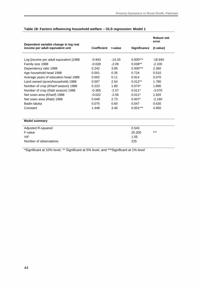
Poverty Dynamics in Rural Sindh, Pakistan
44
Table 18: Factors influencing household welfare – OLS regression: Model 1
Dependent variable change in log real income per adult equivalent unit Coefficient t-value Significance
Robust std. error
(t-value)
Log [income per adult equivalent ]1988 -0.943 -14.33 0.000*** -18.940
Family size 1988 -0.028 -2.09 0.038** -2.100
Dependency ratio 1988 0.242 3.85 0.000*** 2.360
Age household head 1988 0.001 0.35 0.724 0.510
Average years of education head 1988 0.002 0.11 0.914 0.070
Land owned (acres/household) 1988 0.007 2.54 0.012** 1.780
Number of crop (Kharif season) 1988 0.223 1.80 0.074* 1.890
Number of crop (Rabi season) 1988 -0.365 -2.57 0.011* -3.070
Net sown area (Kharif) 1988 -0.022 -2.56 0.011* 1.920
Net sown area (Rabi) 1988 0.049 2.73 0.007* -2.160
Badin taluka 0.075 0.60 0.547 0.630
Constant 1.448 3.46 0.001*** 4.950
Model summary
Adjusted R-squared 0.543
F-value 25.200 ***
VIF 1.55
Number of observations 225
*Significant at 10% level, ** Significant at 5% level, and ***Significant at 1% level
Poverty Dynamics in Rural Sindh, Pakistan
45
Table 19: Factors influencing household welfare – OLS regression: Model 2
Dependence variable change in log real adult equivalent unit income
Coefficient t-value Significance
Robust std. error
(t-value)
Log [income per adult equivalent]1988 -1.038 -16.860*** 0.000 -26.69
Family size 1988 -0.037 -2.800* 0.006 -2.73
Dependency ratio 1988 0.283 2.910** 0.004 2.38
Age household head 1988 0.002 0.520 0.601 0.64
Average years of education head 0.015 0.870 0.387 0.54
Land owned (acres per household 0.008 2.620** 0.010 2.71
Number of crop (Kharif season) 0.270 1.820* 0.071 -2.56
Number of crop (Rabi season) -0.315 -2.170** 0.031 1.9
Net sown area (Kharif) -0.015 -1.020 0.307 1.67
Net sown area (Rabi_ 0.046 2.280** 0.024 -1.08
Badin taluka 0.021 0.170 0.867 0.17
Change variables
Change in family size -0.007 -0.690 0.489 -0.79
Change in dependency ratio -0.005 -0.070 0.946 -0.09
Change in land owned 0.000 0.110 0.916 0.09
Change in operated land(acres per household)
0.006 1.080 0.282 1.25
Change in asset score -0.002 -0.060 0.955 -0.06
Change in share of non-farm income -0.008 -7.450*** 0.000 -3.97
Change in family members working in non-farm income (ten years and above)
0.003 2.660* 0.009 2.39
New crop growers(sunflower) -0.169 -1.210 0.227 -1.55
Change in number of crops(Rabi) -0.039 -0.860 0.389 -0.66
Change in number of crops(Kharif) -0.019 -0.260 0.795 -0.27
Change in net sown area(Rabi) 0.000 0.010 0.991 0.02
Change in net sown area(Kharif) -0.002 -0.180 0.858 -0.22
Constant 2.021 5.050*** 0.000 6.61
Model summary
Adjusted R-squared 0.631
F-value 17.66***
Mean variation Inflation factor (VIF) 2.55
Number of observations 225
*Significant at 10% level, ** Significant at 5% level, and ***Significant at 1% level
The findings from Table 18 are discussed first. The initial level of log income shows a strong
negative coefficient: ceteris paribus it states that income growth was higher for the lower
income groups in 1988 – the lower the income level at 1988, the higher the income growth
over the period. This finding is consistent with other studies (Fields et al., 2003; and Lawson
et al., 2006). In other words, households that were poorer in the baseline period, on average,
Poverty Dynamics in Rural Sindh, Pakistan
46
grew faster (or experienced a slower decline) in terms of income growth than their richer
counterparts.
To find out who were the households in the baseline survey 1987–88 that moved downward
– poor or non-poor – and what was the rate of their income growth over the period, see Table
20A.
Table 20A: Change in log real income per adult equivalent for poor and non-poor households, 1987–88
Mean Std. dev.
Poor (1988) -2.77 0.98
Non-poor (1988) -4.00 0.98
Total -3.52 1.15
Table 20B: Growth rate in log real income per adult equivalent according to poverty status between 1987–88 and 2004–05
Types of poverty Mean
Chronic poor -2.75
Ascending poor -2.81
Descending poor -4.03
Never poor -3.97
Total -3.52
This shows the change in log per adult income between poor and non-poor households in
the baseline period, 1988, based on the relative poverty line. The decline in income was
higher for non-poor (-4.0) than for the poor households (- 2.77) for the baseline survey 1987–
88. This observation also appears consistent with the different categories of poor
households, discussed in the previous section, who moved upward and downward between
1987–88 and 2005. The highest decline in real income growth was for those households who
were descending poor (-4.03) – see Table 20B. It suggests that a majority of the households
who moved downward over the period, were non-poor households in 1987–88, and
experienced a severe decline in their income change.
Moreover, this finding is also consistent when growth rate is measured for consumption
expenditures as changes in log of real consumption expenditures per adult equivalent – see
Table 21A. This shows that decline in mean consumption expenditures was higher for the
Poverty Dynamics in Rural Sindh, Pakistan
47
non-poor (-3.27) than the poor households (-3.21) in 1987–88. Similarly, descending
households experienced the highest decline in their consumption (-3.32) of any category of
poor households in the sample – see Table 21B.
Table 21A: Change in log real consumption per adult equivalent for poor and non-poor households: 1987–88
Mean Std. dev.
Poor (1988) -3.21 0.37
Non-poor (1988) -3.27 0.39
Total -3.25 0.38
Table 21B. Growth rate in log real income per adult equivalent according to poverty status between 1987–88 and 2004–05
Types of poverty Mean
Chronic poverty -3.25
Ascending -3.08
Descending -3.32
Never pPoor -3.25
Total -3.25
The decline in welfare measure was higher for the households who started with a higher
family size in the initial period. This finding is consistent with Fields et al. (2003), Lawson et
al. (2006), and May and Woolard (2007). The change in income was positively associated
with a higher dependency ratio in the baseline period. It indicates that households who had a
higher dependency ratio experienced less decline in their income. This finding is in contrast
with Baulch and McCulloch (1998; 2002). There appear two explanations of this for the
present sample. First, it is more than likely that household members below 15 years of age
and above 64 years were also active in supporting their family income, particularly in
agricultural activities in the study sample. Secondly, it is also likely that family members
below 15 years of age have grown up over the period and are contributing to family income.
Regarding the physical assets, as expected, households who owned more land experienced
a lesser decline in their income.
Agriculture variables, such as the number of crops and the area under cultivation in different
seasons, indicate the importance of farming and seasonal effects on the welfare change of
households. The negative coefficient for the number of Rabi crops shows that those
Poverty Dynamics in Rural Sindh, Pakistan
48
households with a higher number of crops in the Rabi season,experienced a higher decline
in their income than those who had fewer crops in Rabi. However, the same does not appear
to be the case with higher total area cultivated in the Rabi season. It indicates that
households with higher areas of Rabi crops experienced less income fall than the
households with smaller areas. In contrast, a lower number of crops and a high cultivated
area in the Kharif season indicate the opposite. This suggests that households who grew
fewer crops with high cultivated area in Kharif experienced a greater fall in their per capita
income than their counterparts.
It is widely recognised in the literature (Lipton, 1985; Ellis, 1998) that seasonality plays a very
important role in household welfare, and the above findings on the different nature of
seasons and their effects on household welfare support this. A main difference between the
two seasons, Rabi and Kharif, was that one crop, rice, was dominant in Kharif. Nearly two-
thirds of land in Kharif (66 percent) in 1988 was devoted to rice, which is also a main staple
for the population in the study area. The other important crop, in terms of cash income, was
sugarcane, which was cultivated on 18 percent of the area in 1987–88. It takes 12 months for
maturity, and has a high requirement for water. Due to shortage of water and other issues
with sugarcane cultivation, the area under this crop declined by over half (56 percent) in
2004–0518.
In Rabi, the area under sunflower, a new cash crop in the study area, increased
phenomenally. Overall, 43 percent of the cultivated area in Rabi 2004–05 was devoted to
solely to sunflower. A main reason for this was an informed response to water shortage and
economic incentive. Sunflower requires less water, has a shorter growing duration (only
three months compared with over 12 months for sugarcane), and offers high economic
returns, in terms of prices and delivery of payments for sale. One farmer commented that
‘sunflower is like dollars in the pocket – you can sell and receive payment when you like’.
This may explain why the households who had a higher number of crops, together with a low
cultivated area in Rabi season, experienced a greater decline in their income.
The second model takes into account the initial year variables, discussed in Table 18, and
changes over the period. An important finding in Table 19 appears from the labour market.
The strong and negative coefficient for the change in non-farm income share indicates
negative association for income growth. It suggests that households with a large income
share from non-farm employment had less chance of improving their economic welfare. This
requires qualification, as it appears opposite to expectations. However, it appears plausible
when we see it in the context of different environmental shocks to agricultural land and crops
(which may have pushed households from agriculture to the non-farm sector). So, it may be
the case that the higher the share of non-farm income, the lower the increase in economic
18 A number of issues were noted for sugarcane cultivation in the study area, including shortage of water for its cultivation, delay in payment to farmers, and price uncertainty at harvest time.
Poverty Dynamics in Rural Sindh, Pakistan
49
welfare. Moreover, the households who had the higher share of non-farm income were the
landless (they earned over three-quarters of their income from non-farm sources in 1987–88
and 2004–05) and they were mainly engaged in casual and irregular jobs, which were mostly
dependent on agricultural performance. This may also be one of the reasons that incidence
of poverty was very high for labour in 2004–05.
In addition, there also appears to have been a decline in real wages in terms of the
purchasing power of unskilled labour. In 1987–88, an unskilled labourer was earning Rs.32
per day and was able to purchase eight kilograms of wheat flour. In 2004–05, however, a
casual labourer was able to purchase only seven kilograms of wheat flour with a day’s labour
income. This trend of decline in real wages is in complete contrast to the baseline survey.
Alderman and Garcia (1993) argue that real wages (measured in purchasing power of wheat
flour) were higher than in neighbouring countries, and were on a par with urban areas in
Pakistan for that period. This finding of a decline in real wages is consistent with Malik (2005)
and with the Social Policy Development Centre (2004), which also reports decline in real
wages in rural areas of Pakistan for the 1990s.
The positive coefficient for the change in percentage of household members in non-farm
employment indicates a positive association with the change in income. It suggests that
households with high numbers of male family members working in non-farm employment
experienced a smaller fall in income. However, the economic magnitude of this effect
appears to be low, only 0.3 percent. This indicates that although non-farm employment was
positively associated with income growth, its effect was very low. One interpretation of this
could be that what matters most in terms of economic welfare is the nature and type of non-
farm employment, and the number of family members involved in different non-farm earning
activities.
The nature of non-farm employment was mainly seasonal, temporary and dependent on
agricultural performance. Even employment in rice- or flourmills was dependent on crop size:
if the rice or wheat crop was low, this reduced the total days of employment for flourmill
workers. Similarly, persons working as tailors were mainly busy before the two main religious
festivals of the year, Eid ul Fitar and Eid ul Zoha, or sometimes before a special event in
village. So they would have worked for a maximum of six to nine months in a whole year.
This was also the case for household members working in the transport sector. A
combination of factors may thus explain why the magnitude of casual labour income is so
low. This supports Sen’s (1981) observation that in the aftermath of shocks and drought,
there is often an excess supply of non-farm services, such as casual labour, tailors, private
services, etc., with low demand in the local market. In the present case, it appears likely that
households associated with such occupations experienced low demand, and that this led to a
decline in real wages. This strongly emphasises the need for further work on the dynamics of
the labour market, especially non-farm employment, and its impact on poor households and
their economic wellbeing in the rural economy.
Poverty Dynamics in Rural Sindh, Pakistan
50
Both the variables for life-cycle effect, age and education for household head, appear
insignificant. This finding is consistent with Scott (2000), and Fields et al., (2003). A likely
explanation for this comes from Scott’s (2000) argument in the case of Chile. He explains
that in the rural economies of developing countries (where the household is not a nuclear
entity, but lives in a joint and extended household), it is not only the family head’s education
which matters, but that of other family members also becomes more important. A similar
argument can be put forward for not relying solely on the age of the head. The above
findings suggest that agricultural performance has a large influence on household income.
Different shocks in farming have adverse effects on change in income. Households found to
be poor in the initial period are likely, on average, to improve their income position
significantly. At the same time, non-farm employment is also an important source of income
for poor people, and a decline in real wages for casual labour had an adverse effect on poor
households’ income. This emphasis shows there is a need to generate demand for labour-
intensive products and non-farm employment opportunities for poor people.
Poverty Dynamics in Rural Sindh, Pakistan
51
8 Conclusion and policy implications
This paper has investigated the dynamics of poverty in rural Sindh by resurveying
households from an IFPRI longitudinal survey after a gap of over 15 years. The 2004–05
resurvey tracked 95 percent of the 239 panel households, with a very low attrition rate (five
percent). There were no systematic biases for the attriting households. The incidence and
intensity of poverty increased, with 70 percent of households living below the poverty line in
2004–05, compared with 55 percent in 1987–88. Among the different agrarian groups,
poverty was higher among sharecroppers and landless households. These findings were
consistent, using both absolute and relative poverty lines.
Poverty dynamics analysis provided rich insights into poverty mobility. The nature of poverty
was found to be persistent in the study sample. The percentage of households who escaped
poverty was nearly three times lower (12 percent) than the percentage of households who
had fallen into poverty (33.3 percent). Over a quarter of sample households (27.6 percent)
remained in poverty between the two surveys. Overall, income declined by (-19 percent) for
the study sample. The decline in income growth was more severe for the descending poor (-
77 percent) than for the chronically poor (-23.5 percent). The few households who escaped
poverty experienced a nearly threefold increase in their income in 2004–05, compared with
their baseline income.
To complement the above findings, a detailed descriptive analysis, along with the findings
from some qualitative interviews, was also presented. Overall, households who remained
poor in both periods had low per capita incomes, low means for various education
attainments, owned less land and cultivated a small number of crops. The adverse effect of
shocks on household livelihoods was higher for households in the descending poor category.
Households who escaped out of poverty were the only category to experience an increase in
their asset ownership and a marked improvement in human development indicators. Overall,
decline in different indicators of agriculture was lower for this category than the study sample
average. Qualitative interviews suggested that, in addition to decline in income and weather
shocks, there were other factors which caused households to remain in or fall into poverty.
These included cases of health shocks, and mutual support for relatives in times of shocks.
The paper also analysed poverty and major differences between the ‘core panel’ and the
‘new households’. The incidence of poverty was also found to be higher (78 percent) among
the ‘new households’. They had lower incomes and lower asset ownership than the ‘core
panel’. The ‘new households’ were significantly younger, with smaller family size than the
‘core panel’. Secondary education was found to be higher among the ‘core panel’ than the
‘new panel households’.
The analysis of determinants of income change adopted change in log per capita adult
equivalent income as the dependent variable and ran two models. The findings from these
Poverty Dynamics in Rural Sindh, Pakistan
52
were robust and consistent with each other, both when run separately and when combined
together. A main finding from the regression analysis was that income growth was higher for
those with a lower income in the initial period. As per capita income declined in the sample,
the highest decline in log real income was for those households who were non-poor in the
baseline period. The decline in household income was higher for households who started
with a larger family size in the initial period. Households who owned more land experienced a
lower decline in their income. The number of agricultural crops grown and the total area
under cultivation in different seasons were also found to significantly influence household
income. Households with a higher share of income from non-farm activities were found to be
poorer than the others. Real wages for labour declined over the period.
A major finding of the above analysis is that stagnation and absence of growth in agriculture
adversely affects the welfare of rural households, by reducing farm and non-farm income.
The main cause of sharp rises in poverty was shocks in agriculture, along with decline in
non-farm employment opportunities in the study sample. This requires policies to mitigate the
causes of shocks, and more investment in the agriculture sector to enhance sustainable
agricultural growth, particularly for those crops which require less water and provide high
income to farmers, such as sunflower, in the study area. Specific policies should also be
considered to introduce guaranteed employment schemes during the off-peak season in
agriculture, to improve physical rural infrastructure and human capital, and to improve access
to credit and other rural factor markets in order to enhance farm productivity and non-farm
employment in rural areas of Pakistan. Finally, poverty reduction policies need to be
designed according to the nature of the poverty in question, in order to improve the targeting
efficiency of scarce resources in rural areas.
Poverty Dynamics in Rural Sindh, Pakistan
53
References
Adams, Jr. and Richard H. (1993). ’Non-farm income and inequality in rural Pakistan’. Pakistan Development Review, 32(4), 1187–1198.
Adams, Jr., Richard H. (1994). ’Non-farm income and inequality in rural Pakistan: a decomposition analysis’. Journal of Development Studies, 31(1), 110–133.
Adams, Jr., Richard H. and Alderman, H. (1992). ’Sources of income inequality in rural Pakistan: a decomposition analysis’. Oxford Bulletin of Economics and Statistics, 54(4), 591–607.
Adams, Jr. and Richard H. (1995). ’Agricultural income, cash crops and inequality in rural Pakistan’. Economic Development and Cultural Change, 43, 467–492.
Adams, Jr., Richard H.,and He, J. J. (1995). ’Sources of Income Inequality and Poverty in Rural Pakistan’. Research Report No.102. Washington, DC: International Food Policy Research Institute.
Alderman, H. (1996). ‘Savings and economic shocks in rural Pakistan’. Journal of Development Economics, 51, 343–365.
Alderman, H., and Garcia, M. (1993). ’Poverty, Household Food Security, and Nutrition in Rural Pakistan’. Research Report 96. Washington, DC: International Food Policy Research Institute.
Alderman, H., Behrman, J., Kohler, H.P., Maluccio, J. and Watkins, S.C. (2001). ‘Attrition in longitudinal household survey data: some tests for three developing-country samples’. Demographic Research, 5(4), 79–124.
Arif, G. M. (2006). ’Poverty, economic growth, and inequality: a review of Pakistan’s poverty literature’. Background Paper, No. 1.Pakistan Poverty Assessment Update. Islamabad: Asian Development Bank, Resident Mission
Barrett, C.B., Lee, D.R., and McPeak, J.G. (2005) ‘Institutional arrangement for rural poverty reduction and resource conversation’. World Development, 33(2), 193-197,
Baulch, B. and Davis, P. (2008). ’Poverty transitions and livelihood trajectories in rural Bangladesh’. International Journal of Multiple Research Approaches, 2(2), 176–190.
Baulch, B, and Hoddinott, J. (2000). ’Special issue on economic mobility and poverty dynamics in developing countries’. Journal of Development Studies, 36(6), 1–24.
Baulch, B. and McCulloch, N. (1998). ’Being Poor and Becoming Poor: Poverty Status and Poverty Transitions in Rural Pakistan’. Institute of Development Studies Working Paper No. 79. Brighton, UK: Institute of Development Studies.
Baulch, B, and McCulloch, N. (2002). ’Being poor and becoming poor: poverty status and poverty transitions in rural Pakistan’. Journal of Asian and African Studies, 37(2), 168–185.
Chowdhry, D N. (1991). ’Pakistan Rural Household Survey: Documentation of Primary Files’. Washington DC: International Food Policy Research Institute.
Daily Dawn (2006). ’World Bank, UNDP question poverty estimates’. 20 June.
Poverty Dynamics in Rural Sindh, Pakistan
54
Davis, P. (2007). ’Discussions among the Poor: Exploring Poverty Dynamics with Focus Group Discussion in Bangladesh’. Chronic Poverty Research Centre Working Paper No. 84. Manchester, UK: Chronic Poverty Research Centre (CPRC).
Deaton, A. (1997). ‘The Analysis of Household Surveys: A Microeconomic Approach to Development Policy’. Baltimore, MD: John Hopkins University Press.
Deaton, A. (2004). ’Measuring Poverty’. Woodrow Wilson School of Public and International Affairs, Research Program in Development Studies Working Paper 170. New Jersey: Princeton University.
Deaton, A. (1995). ’Data and econometric tools for development analysis’. In J. Behrman and T. N. Srinivason (Eds.), Handbook of Development Economics, Vol. III. Amsterdam, The Netherlands: Elsevier.
Dercon, S. and Shapiro, J. (2007). ‘Moving on, staying behind, and getting lost: lessons on poverty mobility from longitudinal data’. Global Poverty Research Group Working Paper- 075. Available at: http://www.gprg.org/pubs/workingpapers/pdfs/gprg-wps-075.pdf
Dorosh, P. and Malik, S. J. (2006). ’Transitions Out of Poverty: Derivers of Real Income Growth for the Poor in Rural Pakistan’. Paper presented at the International Association of Agricultural Economists Conference, Gold Coasts, Australia, 12–18 August.
Duncan, G. J. and Hill, M S. (1985). ’Concepts of longitudinal households’. Journal of Economics and Social Measurement, 13, 361–375.
Duncan, G. .J. and Hill, M. S. (1988). ’Assessing the quality of household panel data: the case of the panel study of income dynamics’. Journal of Business and Economic Statistics, 7(4), 441–452.
Duncan, G. J. and Kalton G. (1987). ’Issues of design and analysis of surveys across Time’. International Statistical Review, 55(1), 97–117.
Ellis, F. (1998). ’Survey article: household strategies and rural livelihood diversification’. Journal of Development Studies, 35(1), 1–38.
Ellis, F. (2000). Rural Livelihood and Diversity in Developing Countries. Oxford, UK: Oxford University Press.
Fields, G. S., Cichello, P. L., Freije. S., Menedez, M. and Newhouse, D. (2003). ‘Household income dynamics: a four country story’. Journal of Development Studies, 40(2), 30–54.
Foster, J., Greer, J., and Thorbecke, E. (1984). ‘A class of decomposable poverty measures’. Econometrics, 52(3), 761–766.
Gaiha, R. (1988). ‘Income mobility in rural India’. Economic Development and Cultural Change, 36(2), 279–302.
Gazdar, H. (2007). Rural Economy and Livelihoods in Pakistan’. Thematic paper prepared under TA4319. Islamabad: Asian Development Bank.
Gazdar, H. (2002). ’A Qualitative Survey of Poverty in Rural Pakistan: Methodology, Data, and Main Findings’. Mimeo.
Ghausi, S. (2006). ’Woes of rural Sindh’. Daily Dawn, 20 November.
Poverty Dynamics in Rural Sindh, Pakistan
55
Government of Pakistan (2005–06). ‘Pakistan Social and Living Standard Measurement Survey’. Islamabad: Federal Bureau of Statistics.
Government of Pakistan (2006-07). ‘Economic Survey of Pakistan’. Islamabad, Pakistan: Ministry of Finance.
Hume, D and Shepherd, A. (2003). ‘Conceptualizing chronic poverty’. World Development, 31(3), 403-427
Hussain, A. (2003). ‘Poverty, Growth and Governance’. Pakistan National Human Development Report. United Nation Development Program, Pakistan. Oxford, UK: Oxford University Press.
Jafri, S. M. (2002). ’Issues in Measuring Poverty in Pakistan’. Working Paper No. 2. Islamabad: Centre of Research on Poverty Reduction and Income Distribution (CRPRID).
Jamal, H. (2002). ’On the estimation of absolute poverty line: an eremitical approach’. Lahore Journal of Economics, 7, 77–92.
Jamal, H. (2007). ’Updating Poverty and Inequality Estimates: 2005 Panorama’. Research Report, No. 69. Karachi: Social Policy and Development Centre (SPDC).
Jamal, H., and Lohano, H, R. (2008). ’Understanding Rural Poverty Dynamics: Case of Poorest Distinct of Sindh, Pakistan’. Research Report, 78. Karachi: Social Policy and Development Centre (SPDC).
Khan, M, H. (2006). Agriculture in Pakistan: Change and Progress in Pakistan. Lahore: Vanguard Publications.
Kurosaki, T. (2006a). ’Consumption vulnerability to risk in rural Pakistan’. Journal of Development Studies, 42(1), 70–89.
Kurosaki, T. (2006b). ’The measurement of transient poverty: theory and application to Pakistan’. Journal of Economic Inequality, 4(3), 325–345.
Lanjouw, P. and Stern, N. (1998). ’Poverty in Palanpur’. In P. Lanjouw and N. Stern (Eds.), Economic Development in Palanpur: Over Five Decades. Oxford, UK: Oxford University Press.
Lawson, D., McKay, A. and Okidi, J. (2006). ’Poverty persistence and transitions in Uganda: a combined qualitative and quantitative analysis’. Journal of Development Studies, 42(7), 1225–1251.
Leon, I. U. and Dercon, S. (2008). ’Survey Attrition and Attrition Biases in Young Lives’. Young Lives, Technical Note 5. Available at: http://www.younglives.org.uk. Accessed 1 October 2009.
Lipton, M. (1985). ’Land Assets and Rural Poverty’, World Bank Staff Working Paper, No. 744. Washington, DC: The World Bank.
Lohano, H. R. (2006a). ’Income Mobility in Rural Sindh’. Research paper prepared for Collective for Social Research, Karachi, and Asian Development Bank, Islamabad.
Lohano, H. R. (2006b). ’Forgotten but Not Lost: Resurvey of Longitudinal Households after 15 Years in a Developing Country’. Paper prepared for International Conference on the Methodology of Longitudinal Surveys (MOLS), Institute of Social and Economic Research (ISER), University of Essex, Essex, UK, 12-14 July.
Poverty Dynamics in Rural Sindh, Pakistan
56
Lohano, H. R. (2009). ‘Agricultural Growth and Poverty Dynamics in Rural Pakistan: Evidence from Longitudinal Survey for Sindh Province (1987–88 to 2004–05)’. PhD dissertation (pp.63–94). University of Bath, UK.
Malik, S. (2008). ’How credible is national data’. Daily Dawn, 6 February.
Malik, S. J. (2005). ’Agricultural Growth and Rural Poverty: A Review of the Evidence’. Working Paper No. 2. Pakistan Resident Mission, Islamabad: Asian Development Bank.
May, J. and Woolard, I. (2007). ’Poverty Traps and Structural Poverty in South Africa: Reassessing the Evidence from Kwazulu-Natal’. Chronic Poverty Research Centre Working Paper No. 82. Manchester, UK: Chronic Poverty Research Centre (CPRC).
McCulloch, N. and Baulch, B. (1999). ‘Distinguishing Chronically from the Transitorily Poor: Evidence from Rural Pakistan‘. Institute of Development Studies Working Paper No. 97. Brighton, UK: Institute of Development Studies.
McCulloch, N. and Baulch, B. (2000). ‘Simulating the impact of policy upon chronic and transitory poverty in rural Pakistan’. Journal of Development Studies, 36(6), 100-130
McKay, A. (2000). ’Should the survey measure total household income? In M. Grosh and P. Glewwe (Eds.), Designing Household Survey Questionnaire for Developing Countries: Lessons from 15 Years of the Living Standard Measurement Study (chapter 17). Washington, DC: The World Bank.
McKay, A. (2007). ‘Introduction to methods for analysing the distributional pattern of growth’. In Grimm, M., Klasen, S. and McKay, A. (Eds.), Determinants of Pro Poor Growth: Analytical Issues and Findings from Country Cases (chapter 2). Basingstoke: Palgrave Macmillan.
Mustafa, Z. (2007). ’What hurts is the rich-poor divide’. Daily Dawn, 25 April.
Narayan, D. and Petesch, P. (Eds) (2007). ‘Moving Out of Poverty: Cross-Disciplinary Perspectives on Mobility’, Volume 1. Washington, USA: World Bank.
Oxford Policy Management (OPM) (2003). ’Pakistan Integrated Household Survey: How Poverty Increased’. Report prepared for Federal Bureau of Statistics, Islamabad, Pakistan.
Pasha, H. and Hasan, T. (1982). ’Development ranking of districts in Pakistan’. Pakistan Journal of Applied Economics, 1(winter), 157–192.
Ravallion, M. (1993). ‘Poverty Comparisons: A Guide to Concepts and Measures’, Living Standards Measurement Study Working Paper No. 88. World Bank, Washington, DC
Ravallion, M. (1996). ’Issues in Measuring and Modelling Poverty’, Policy Research Working Paper No. 1615. Washington, DC: The World Bank.
Scott, C. (2000). ‘Mixed fortunes: a study of poverty mobility among small farm households in Chile, 1968–86’. Journal of Development Studies, 36 (6), 155–180.
Sen, A. (1981). ’Poverty and famines: an essay on entitlements and deprivation’. Oxford, UK: Oxford University Press.
Sen, B. (2003). ‘Drivers of escape and descent; changing household fortunes in rural Bangladesh’. World Development 31(3), 513–534.
Poverty Dynamics in Rural Sindh, Pakistan
57
Shorrocks, A. F. (1978a). ’Income inequality and income mobility’. Journal of Economic Theory, 19, 376–393.
Shorrocks, A.F. (1978b). ’The measurement of mobility’. Econometrica, XLV( 5), 1013–1024.
Social Policy and Development Centre (SPDC) (2004). ’Combating Poverty: Is Growth Sufficient?’. Annual Review. Karachi: Pakistan SPDC and Oxford University Press, Pakistan.
Sumater, B. (1995). ’Credit Constraints and their Impact on Risk Bearing and Pre-cautionary Savings: A Case Study from Rural Pakistan’ (pp. 9–10). PhD dissertation. Baltimore, MD: Johns Hopkins University.
Sundrum, R. M. (1990). ’Some problems in income measurement’. In Income Distribution in Less Developed Countries. London: Routledge.
Thorbecke, E. (2003). ’Conceptual and Measurement Issues in Poverty Analysis‘. Paper prepared for the WIDER conference on ‘Inequality, Poverty and Human Well-being’, Helsinki, Finland, 30-31 May.s
Woolard I. and Klasen S. (2005). ‘Determinants of income mobility and household poverty dynamics in South Africa’. Journal of Development Studies, 41(5), 865–897.
Wooldridge, J. M. (2006). Introductory Econometrics: A Modern Approach. Cincinnati, OH: South-Western.
World Bank (2002). ‘Pakistan Poverty Assessment: Vulnerabilities, Social Gaps, and Rural Dynamics’. Report No. 24295-PAK. Washington, DC: World Bank.
World Bank (2007). ‘Pakistan Promoting Rural Growth and Poverty Reduction’. Report No. 39303PK. Washington, DC: World Bank.
World Development Report (2008). ’Agriculture for Development’. Washington, DC: World Bank.
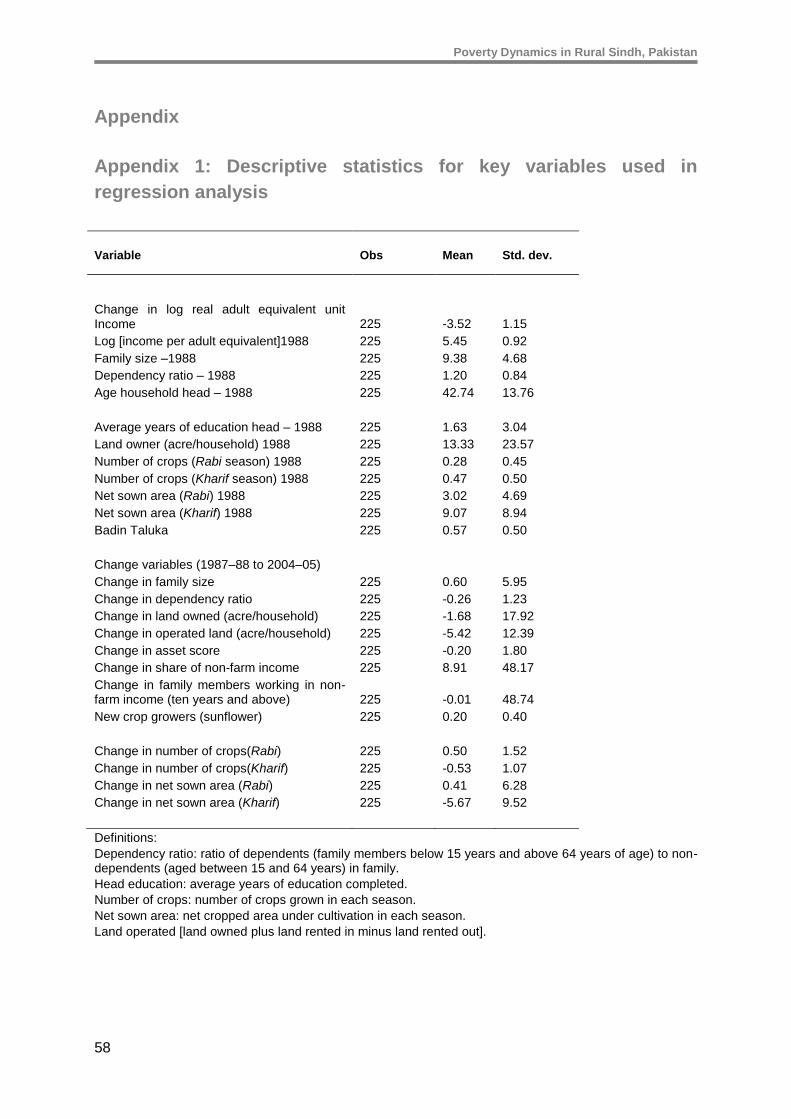
Poverty Dynamics in Rural Sindh, Pakistan
58
Appendix
Appendix 1: Descriptive statistics for key variables used in
regression analysis
Variable Obs Mean Std. dev.
Change in log real adult equivalent unit Income 225 -3.52 1.15
Log [income per adult equivalent]1988 225 5.45 0.92
Family size –1988 225 9.38 4.68
Dependency ratio – 1988 225 1.20 0.84
Age household head – 1988 225 42.74 13.76
Average years of education head – 1988 225 1.63 3.04
Land owner (acre/household) 1988 225 13.33 23.57
Number of crops (Rabi season) 1988 225 0.28 0.45
Number of crops (Kharif season) 1988 225 0.47 0.50
Net sown area (Rabi) 1988 225 3.02 4.69
Net sown area (Kharif) 1988 225 9.07 8.94
Badin Taluka 225 0.57 0.50
Change variables (1987–88 to 2004–05)
Change in family size 225 0.60 5.95
Change in dependency ratio 225 -0.26 1.23
Change in land owned (acre/household) 225 -1.68 17.92
Change in operated land (acre/household) 225 -5.42 12.39
Change in asset score 225 -0.20 1.80
Change in share of non-farm income 225 8.91 48.17
Change in family members working in non-farm income (ten years and above) 225 -0.01 48.74
New crop growers (sunflower) 225 0.20 0.40
Change in number of crops(Rabi) 225 0.50 1.52
Change in number of crops(Kharif) 225 -0.53 1.07
Change in net sown area (Rabi) 225 0.41 6.28
Change in net sown area (Kharif) 225 -5.67 9.52
Definitions:
Dependency ratio: ratio of dependents (family members below 15 years and above 64 years of age) to non-dependents (aged between 15 and 64 years) in family.
Head education: average years of education completed.
Number of crops: number of crops grown in each season.
Net sown area: net cropped area under cultivation in each season.
Land operated [land owned plus land rented in minus land rented out].
Poverty Dynamics in Rural Sindh, Pakistan
59
Appendix 2: Methodology for constructing income aggregates.
To maintain consistency and comparability with the IFPRI baseline survey, this study follows
the income estimation methodology used by Alderman and Garcia (1993) and Adams and
Jane (1995). Household income was divided into six main sources: net crop profit, farm
wages, livestock income, non-farm, rental, and income from transfers. Income definitions and
aggregates are explained below.
i. Crop income
This is net income from three sources: crop profits, crop by-products, and orchards. Income
from crops includes net income from all crops produced in Rabi and Kharif seasons, and
imputed value of home production for these crops. Net crop income subtracts costs incurred
on production, including fertilisers, seeds, water purchase, hired labour, tractor and thresher.
Income from by-products is the imputed value of by-products for wheat and rice straw.
Income from orchard is net income from sale of fruits.
ii. Farm wages
These are earnings for family members, female and male, aged ten years and above,
working on others’ farms for different types of farm labour, such as crop cutting, sowing, land
preparation, etc. In most cases, farm wages were paid in-kind. Money estimates of these
were obtained from the respondents.
iii. Income from livestock
Income from livestock includes sale of livestock dairy products, including milk, yogurt, ghee,
eggs and chicken. Income from sale of livestock is treated as capital item and so excluded.
A main reason for adopting this definition was difficulties faced in the computation of
livestock expenditures on feeding and other costs. To maintain consistency, the same
definition is used for both surveys, 1987–88 and 2004–05.
iv. Rental income
This consists of four types of income. Firstly, net income from leasing out land for
sharecropping, which is gross value of crops received in kind from tenants to land owners
according to their share in production. Secondly, income received from leasing out land at a
fixed rent. Thirdly, net income from renting out machinery and capital equipment, which is
gross income received from renting out tractor, thresher, bullock power, etc., minus cost
Poverty Dynamics in Rural Sindh, Pakistan
60
incurred on maintenance. Fourthly, income received from renting out off-farm assets, such as
urban property-buildings and shops at farm or in urban area.
v. Non-farm income
Non-farm income consists of a wide range of occupations, by female and male household
members, aged ten years and above. It was divided into four exclusive categories. Firstly,
income earned from private-sector employment. This is mainly salary income received from
flour, rice, and sugar mills in the study area; working at small garages, tea shops, and
occasionally in the transport sector. Most of the activities in this category were paid by
monthly salary. Secondly, income earned from labour wage. This includes a wide range of
labour activities, such as daily wages labour, working in construction, transport, shepherd,
Beri making, and other economic activities in the local area. Female members in this
category were mainly working at home-based economic activities, such as embroidery ng),
handicraft and stitching.. Thirdly, net income earned from self-employment, which includes
own business, joint household economic activity, such as local shops, selling fertilisers,
vegetables, fish farming, tailoring, livestock trading, etc. Fourthly, income received from
government jobs.
It is important to note that most of the non-farm income sources and jobs in the study area,
except government employment, were seasonal in nature and apparently were highly
dependent on the performance of agriculture. In the estimation of non-farm income, special
consideration was taken to account for the nature of jobs and seasonality in the year. For all
the sources of non-farm income, except government employment, in cases for which
households did not provide information on annual income, it was calculated as nine months
instead of a full year for both the surveys.
vi. Transfer income
Transfer income consists of six sources of income: remittances received from family
members working domestically and internationally; government pension; ushr and zakat
(religious donations); cash transfers, i.e., the cash value of grain received from relatives and
others as transfers; and cash values of appliances (such as TVs and refrigerators) received
from family members. A surprising feature of transfer income was the low share of remittance
income from domestic or other countries. None of the household members were working
outside the country in 1987–88, and there was only one household member working abroad
in 2004–05.
The Chronic Poverty Research Centre (CPRC) is an international partnership of universities, research institutes and NGOs, with the central aim of creating knowledge that contributes to both the speed and quality of poverty reduction, and a focus on assisting those who are trapped in poverty, particularly in sub-Saharan Africa and South Asia.
Partners: Bangladesh Institute of Development Studies (BIDS), Bangladesh Development Initiatives, UK Development Research and Training, Uganda Economic Policy Research Center, Uganda FIDESPRA, Benin HelpAge International, UK Indian Institute of Public Administration, India IED Afrique, Senegal Institute of Development Studies, UK Overseas Development Institute, UK Programme for Land and Agrarian Studies, South Africa University of Legon, Ghana University of Manchester, UK University of Sussex, UK
Contact: [email protected] © Chronic Poverty Research Centre 2009
www.chronicpoverty.org