The input-output framework and modelling assumptions: considered from the point of view of the economic circuit

May 2007

Luc Avonds1, la@plan.be

Federal Planning Bureau

Avenue des Arts 47-49

1000 Brussels Belgium

(http://www.plan.be)

Abstract - The immediate cause for this paper is another paper presented for the first

time by Professor de Mesnard at the 14th International Input-Output Conference and

published in the Journal of Regional Science in 2004. According to him input-output

models derived from supply and use tables by means of the product technology

assumption fail in terms of the economic circuit (the chaining from final demand to total

output in a traditional Leontief input-output system). I have studied his paper(s)

intensively and I have, for several reasons, to make serious considerations to his point

of view. My paper is not merely a reply to de Mesnard but it tries also to give a more

general approach of the SNA input-output framework in terms of the economic circuit.

When considering explicitly make and use tables in the economic circuit make and use

1 The author is a member of the Belgian Federal Planning Bureau. The views expressed in this paper are those of the

author and do not necessarily reflect those of the Federal Planning Bureau.

tables should be considered in every step of the economic circuit. The mathematical

series of this make and use tables in every step should converge to the “total” make and

use tables as given in the national accounts. When combining technology assumptions

(product technology, industry technology) with output structure assumptions (constant

product-mix, constant market shares) different versions of the economic circuit are

obtained. The make, use and product-by-product tables obtained in every step will differ

according to the chosen assumptions but the make and use tables have to converge to

the tables integrated in national accounts. In this way different consistent versions of the

economic circuit under the assumption of product technology can be obtained. Professor

de Mesnard seems to reduce product technology to the special case of a constant

product-mix but even when one considers this special case his statement raises

questions. When the output structure assumptions are extended to sales structure

assumptions (fixed industry sales structures and fixed product sales structures) industry-

by industry tables can be obtained in every step of the economic circuit. This has given

me some interesting insights. The industry-by-industry table based on the assumption of

a fixed product sales structure does not appear to be invariant of the technology

assumption (what some people claim) when it is used for impact analysis. Some

attention is also given to the practical aspects of input-output compilation. Assumptions

should not only be considered from a theoretical point of view but attention should also

be paid to the statistical framework in which they are applied.

.

Jel Classification – C67

Keywords – Input-output tables, supply and use tables, technology assumptions

Acknowledgements -

1

Introduction

The choice of which input-output model to derive from underlying supply and use

tables is usually made on the basis of theoretical and/or practical considerations.

The first choice is that between so-called product by product or industry by industry

tables. Product by product tables describe the input structure of (analytically

constructed) homogeneous branches in terms of product groups and value added and

also the final uses by category of these product groups. Industry by industry tables

describe market relations: the intermediary deliveries between statistical units grouped

in industries according to their principal activity, the value added of these industries and

their deliveries to the categories of final demand.

When product by product tables are chosen the next step is the choice of the technology

assumption. Several modelling assumptions have been proposed over the last decades

but the choice is mostly limited between two assumptions: product technology (a given

product always has the same input structure irrespective in which industry it is

produced) or industry technology (the input-structure of an industry remains invariant

irrespective of its product-mix). There is a lot of disagreement about which of these two

assumptions is the most preferable. There is considerably less controversy, in fact none,

about which assumption is preferable when industry by industry tables are chosen. But

the choice between product by product tables or industry by industry tables as official

tables forming part of national accounts is the subject of an international controversy.

The SNA 68 and its accompanying input-output manual (United Nations, 1968 and

1973) presented different versions of input-output tables but gave no preference to one

of them. The ESA 70 and 79 national accounting systems of the EU (Eurostat, 1979)

included input-output tables based on homogeneous branches (formally product by

2

product tables) but they did not give any indication of how these tables should be

constructed starting from basic data (these systems did not include supply and use

tables).

Two Dutch academics, Kop Jansen and ten Raa, did put forward four axioms of

desirable properties of input-output tables (Kop Jansen and ten Raa, 1990):

• material balance (supply = use)

• financial balance (output = costs)

• scale invariance (the technical coefficients should be invariant to proportional

variations of the input requirements and outputs of the industries)

• price invariance (the constant price estimate of the input-output table should be

invariant to price fluctuations)

As we understand these are the axioms on which traditional input-output analysis by

means of Leontief equations is based. When considering input-output tables in a system

of supply and use tables only the product technology fulfils the four desirable

properties, industry technology fulfils only the first one. This means that if one wants to

perform traditional input-output analysis product by product tables based on product

technology should be compiled. It is logical to use a model that is in conformity with

the axioms on which the analysis is based on, or to make an estimate that approaches

this model as much as possible. An article published in the Economic Systems Research

journal in 2003 treated this matter further but it did not contain any drastic changes

compared with the first paper (ten Raa and Rueda-Cantucha, 2003).

The SNA 93 (United Nations et al., 1993) contains only product by product tables and

showed preference for product technology, referring to the 4 axioms of desirable

proportions put forward by ten Raa and Kop Jansen). The accompanying input-output

3

manual (United Nations, 1999) presents different kind of input-output tables (like its

predecessor) but also with a preference for product technology. The ESA 95 also only

contains product by product tables. These are in fact the tables that the member states of

the EU are (legally) obliged to transmit to Eurostat. But it showed no preference for

any type of technology assumption. An accompanying input-output manual was written

but unfortunately not published because of disagreements between the member states of

the EU over which kind of input-output table is preferable as part of national accounts

(Beutel, 2005).

At the 14th International Input-Output Conference a new critique of a theoretical nature

against the product technology was formulated by Professor de Mesnard of the

University of Dijon (the author of this paper did not attend this session). According to

him the interpretation of the product technology fails in terms of the economic circuit

(de Mesnard, 2002). A definitive version of his paper has been published in the Journal

of Regional Science (de Mesnard, 2004b). The use of the term “economic circuit”

should be interpreted as the chaining of intermediate demand caused by an initial impact

on final demand in the traditional Leontief input-output system. He claims that product

technology breaks the economic circuit because of the emergence of negative outputs at

every step of the economic circuit and should be abandoned in favour of industry

technology.

At the same conference more opposition to product technology could be heard from B.

Thage of Statistics Denmark (Thage, 2002a). He claims that his critique of product

technology is more of a pragmatic nature and based on a long established practice.

Statistics Denmark has been in fact applying the SNA input-output system for decades

with supply and use tables as the core of the national accounts (Thage, 1986). The

4

objections of Statistics Canada against product technology are of the same nature (Lal,

1999). Both prefer industry by industry tables as part of national accounts for practical

reasons but B. Thage welcomed de Mesnard’s critique as an extra argument (Thage,

2002b).

This critique was also mentioned in a paper of the US Bureau of economic Analysis

(Guo et al. ,2002) Up to 1992 at least, the US Benckmark input-output tables were

partly calculated by a mix of a transfer method being like (but not exactly equal to) the

product technology model and industry technology. The authors of this paper mentioned

de Mesnard critique in a neutral way in a general overview of the input-output literature

on technology assumptions.

The author did attend the presentation by de Mesnard of the second version of his paper

at the intermediate input-output conference in Brussels in 2004 (de Mesnard, 2004a).

The audience consisted mainly of CGE modellers (input-output and CGE modelling

was the subject of the conference) clearly not acquainted with the methodological and

practical aspects of the compilation of input-output systems and there was hardly any

reaction. As far is I know the authors who have studied and defended up to a certain

degree the product technology model in the past have not replied to de Mesnard

critique. His statements seem to be taken automatically for granted or simply ignored,

neither of which we consider being a good attitude.

The author is a member of the Belgian institute charged with the compilation of the

“official” Belgian input-output tables (this is my principal activity, my secondary

activity consist in using these tables). In this capacity the Belgian “input-output team” is

rather a user and not a developer of methodologies but a user of methodologies should

5

be interested in the theoretical back-ground of these methodologies. From this point of

view I have an undertaken a study of de Mesnard’s critique because:

• his paper does not contain elaborated examples

• by my knowledge people far more suitable to react have not done this (to my

surprise until now not even one article in the ESR journal has mentioned de

Mesnard statements1).

We have made exercises with different versions of the input-output systems considering

supply, use, product by product and industry and industry tables under different

modelling assumptions. We have only considered the Leontief model and not the Gosh

model (as far as I know this model has never been used by my institution and it is in

general considered as a curiosity). Before we show these exercises, let us first repeat

how traditional Leontief input-output systems function.

1 The article of Ten Raa and Rueda-Cantuche mentioned several papers presented at the Montreal input-output

conference but not that one of de Mesnard.

6

1. Traditional Leontief input-output models

The representation of the economic circuit in case of the traditional Leontief input-

output model is straightforward.

In the traditional Leontief input-output model, each industry produces only one product

and each product is only produced by one industry. In other words, the use table is

already an input-output table. The statement “each industry produces only one product

and each product is only produced by one industry” should be toned down in practice.

The pure concept of a product can only be reached by a level of detail of the underlying

product and industry classifications that is not applicable in reality. The original

statement should therefore be mitigated to: each industry is already a homogeneous

branch; it produces only products that come under the activity corresponding to its label

in the underlying industry classification.

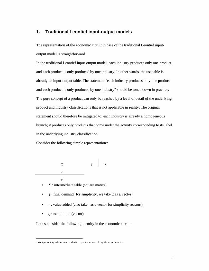
Consider the following simple representation2:

X f q

v′

q′ • X : intermediate table (square matrix)

• f : final demand (for simplicity, we take it as a vector)

• v : value added (also taken as a vector for simplicity reasons)

• q : total output (vector)

Let us consider the following identity in the economic circuit:

2 We ignore imports as in all didactic representations of input-output models.

7

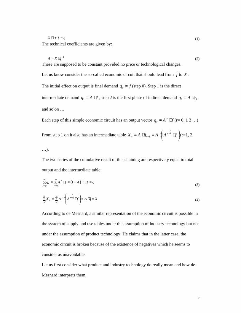
qfiX =+⋅ (1)The technical coefficients are given by:

1ˆ −⋅= qXA (2)These are supposed to be constant provided no price or technological changes.

Let us know consider the so-called economic circuit that should lead from f to X .

The initial effect on output is final demand fq =0 (step 0). Step 1 is the direct

intermediate demand fAq ⋅=1 , step 2 is the first phase of indirect demand 12 qAq ⋅= ,

and so on …

Each step of this simple economic circuit has an output vector fAq rr ⋅= (r= 0, 1 2 …)

From step 1 on it also has an intermediate table

⋅⋅=⋅= −

−

^1

1ˆ fAAqAX rrr (r=1, 2,

…).

The two series of the cumulative result of this chaining are respectively equal to total

output and the intermediate table:

( ) qfAIfAqor r

rr =⋅−=∑ ∑ ⋅= −∞

=

∞

=

1

0 (3)

XqAfAAXr r

rrr =⋅=∑ ∑

⋅⋅=

∞

=

∞

=

− ˆ1 1

^1

(4)

According to de Mesnard, a similar representation of the economic circuit is possible in

the system of supply and use tables under the assumption of industry technology but not

under the assumption of product technology. He claims that in the latter case, the

economic circuit is broken because of the existence of negatives which he seems to

consider as unavoidable.

Let us first consider what product and industry technology do really mean and how de

Mesnard interprets them.

8

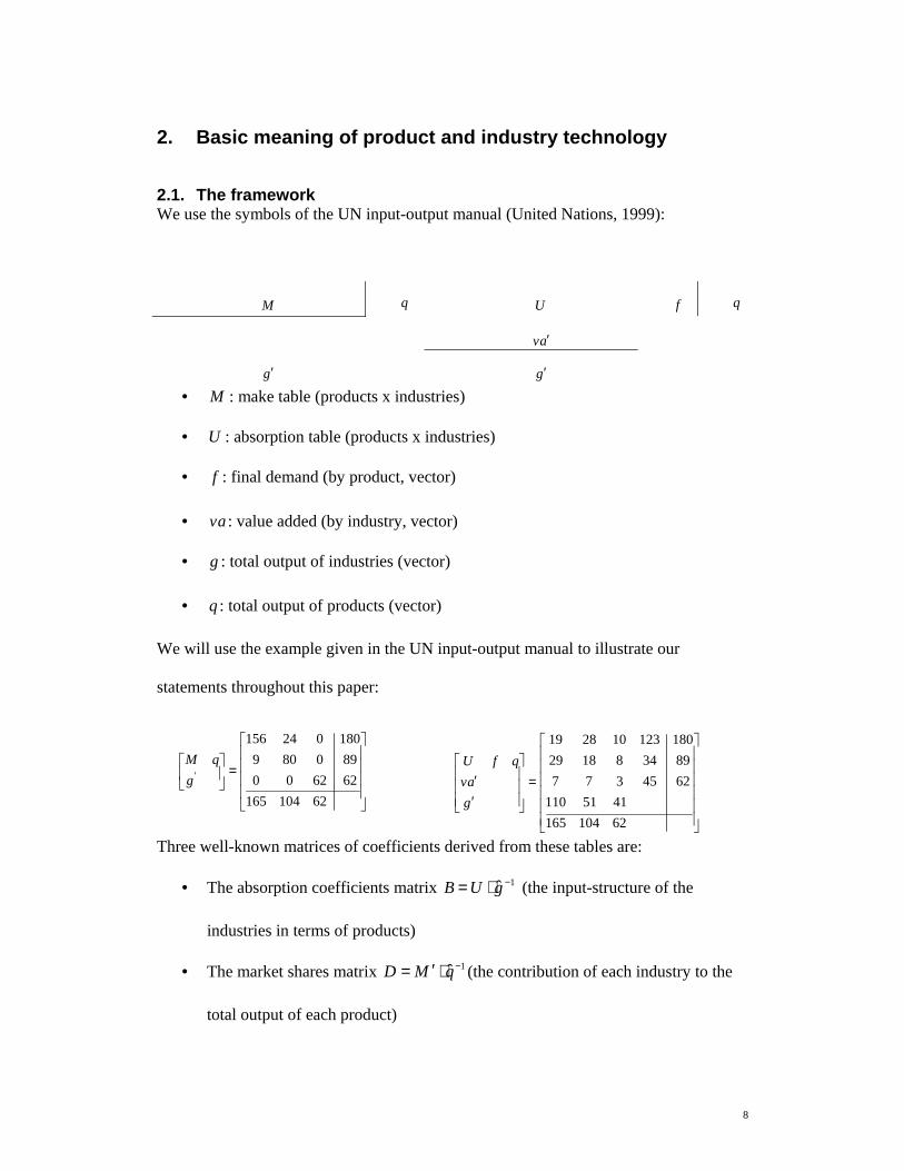
2. Basic meaning of product and industry technology

2.1. The framework We use the symbols of the UN input-output manual (United Nations, 1999):

M q U f q

av ′

g′

g′

• M : make table (products x industries)

• U : absorption table (products x industries)

• f : final demand (by product, vector)

• va : value added (by industry, vector)

• g : total output of industries (vector)

• q : total output of products (vector)

We will use the example given in the UN input-output manual to illustrate our

statements throughout this paper:

=

62104165626200890809

180024156

'gqM

=

′′

621041654151110

6245377893481829

180123102819

gav

qfU

Three well-known matrices of coefficients derived from these tables are:

• The absorption coefficients matrix 1ˆ −⋅= gUB (the input-structure of the

industries in terms of products)

• The market shares matrix 1ˆ −⋅′= qMD (the contribution of each industry to the

total output of each product)

9

• The product-mix matrix 1ˆ −⋅= gMC (the share of each product in the total output

of each industry)

=

%8.4%7.6%2.4%9.12%3.17%6.17%1.16%9.26%5.11

B

=

%0.100%0.0%0.0%0.0%9.89%3.13%0.0%1.10%7.86

D

=

%0.100%0.0%0.0%0.0%9.76%5.5%0.0%1.23%5.94

C

The make and use tables above can be considered as the matrices compiled for the

national accounts. The matrices B ,C and D are not always constant by definition.

Whether or not they are considered to be constant (to remain equal to the values derived

from the national accounts) during each step of the economic circuit, or when

performing impact analysis, depends on the assumptions made to derive symmetric

input-output tables.

Product and industry technology are two different assumptions on the base of which two

different product-by-product tables can be derived from the make and absorption tables.

2.2. Product technology Product technology assumes that a given product always has the same input structure

irrespective where it is produced. It means that a given product x product matrix of

technical coefficients A is hidden behind the “observed” make and absorption tables

according to which all industries produce their different (principal and secondary)

products. This means that:

MAU ⋅= (5)This matrix A is in fact Leontief type matrix which is supposed to lie at the base of the

make and absorption tables. So it is no more logical that the product technology model

meets all the so-called Kop Jansen-ten Raa conditions without any further stipulations,

while the other treatments of secondary products do not.

Equation (5) can also be written as:

10

CAB ⋅= (6)This formula seems to have caused a lot of confusion since some seem to suppose that

the invariability of A rests on the invariability of matrices B and C while it is assumed

to be constant by nature (Konijn, 1994).

A constant product-mix matrix (which is often erroneously given as the definition of

product technology) is by no means necessary. If C varies A remains invariable by

definition, and B adapts itself to the new product-mix. Richard Stone clearly did not

mention a constant product-mix in part 3 of A Program for Growth (Stone et al., 1963).

Neither the SNA 93, nor the accompanying input-output manual mentions a constant

product-mix explicitly as a condition for product technology (they neither say that

C has to be invariable, nor that it can be variable). The SNA 68 and its accompanying

input-output manual (United Nations, 1973) did not either when they defined product

technology. But they declared industry-by-industry tables characterised by a constant

product-mix as “the industry-by-industry variant of product-technology”. This is in the

first place not right (see below) and seemed in the second place to have caused a lot of

confusion.

Product technology was identified with a constant product-mix in the 1985 edition of

Miller and Blair “Input-output analysis: foundations and extensions” (Miller and Blair,

1985). This book is considered as a standard work and de Mesnard has taken over their

definition of product technology. Does his critique of product technology still holds if

we accept the more general definition of product technology given by Konijn?

The pure concept of product technology can only be reached by a level of detail of the

underlying product and industry classifications that is not applicable in reality. The

strict definition is therefore in reality mitigated to: if an industry has a secondary

11

production (it produces products that come under the activity corresponding to the label

of another industry in the underlying industry classification) the input-structure of this

secondary production is equal to the input-structure of the total principal production of

this other industry. This means that strictly speaking not a product x product table but a

homogeneous branch x homogeneous branch table is calculated. This is an

approximation of a product x product table but if it is calculated by means of matrix

calculation it continues to satisfy the Kop Janssen-ten Raa conditions.

A can be calculated by 1−⋅ MU or 1−⋅CB . Application of product technology requires

the number of products and industries to be equal: mathematically this is necessary for

the inversion of the matrices C or M , economically this means that the estimation of the

input-structure of a homogeneous branch requires a corresponding industry that is the

principal producer of the products characterising that homogeneous branch. The

technology matrix of the Leontief system is namely homogeneous, symmetrical (this

term is generally used while according to Almon “symphisic” is more appropriate,

Almon, 2000) and square and the assumption of product technology is an attempt to

implement input-output analysis by means of Leontief equations into a framework with

supply and use tables. This means that the working format of the make and use tables

has to be aggregated to square matrices with dimension equal to the number of

industries.

In the SNA input-output manual A is equal to:

=

%8.4%5.7%1.4%9.12%2.17%6.17%1.16%9.31%3.10

A

12

2.3. Industry technology Industry technology means that the input-structure of an industry remains invariant

irrespective of its product-mix. This means that B is matrix of constants given no price

or technological changes. Without any additional condition an invariable matrix of

product-by-product technical coefficients simply does not exist.

According to the assumption of industry technology, the input-structure of a product in

terms of other products is a weighted average of the input-structure of the industries

where it is produced as a principal or secondary activity:

=⋅

%8.4%5.6%6.4%9.12%3.17%5.17%1.16%4.25%6.13

DB

Since B is a matrix of constants by definition, DB ⋅ can only be invariable if D is a

matrix of constants.

The derivation of a product by-product matrix of invariable technical coefficients under

industry technology needs the additional assumption of constant market shares, while

the assumption of product technology does not need the additional assumption of a

constant product-mix (invariability of C ).

The matrix multiplication DB ⋅ looks like a Leontief matrix but this is only apparent

since the technology matrix at the base of the system is the invariable matrix B which is

clearly not a Leontief matrix. So it is no wonder that the matrix DB ⋅ does not meet all

the Kop Jansen-Ten Raa conditions.

The SNA 93 judges the industry technology as highly implausible, as Richard Stone et

al. already did in 1963 (although they admitted that industry technology can be a better

approximation if some industries are too aggregated in the working format of the supply

and use tables, Stone et al., 1963). Almon did not mince his words and considers the

13

official recommendation by international organizations and use by numerous statistical

offices of industry technology “little short of scandalous” (Almon, 1998).

14

3. The economic circuit of the input-output framework

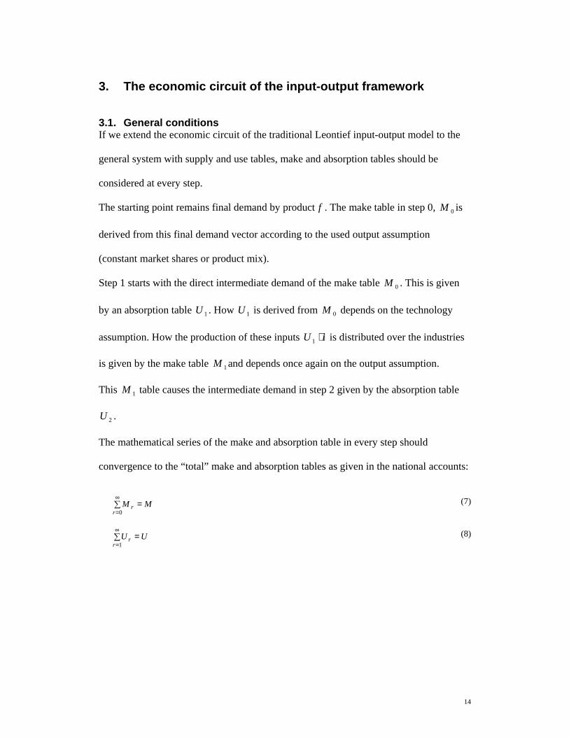
3.1. General conditions If we extend the economic circuit of the traditional Leontief input-output model to the

general system with supply and use tables, make and absorption tables should be

considered at every step.

The starting point remains final demand by product f . The make table in step 0, 0M is

derived from this final demand vector according to the used output assumption

(constant market shares or product mix).

Step 1 starts with the direct intermediate demand of the make table 0M . This is given

by an absorption table 1U . How 1U is derived from 0M depends on the technology

assumption. How the production of these inputs iU ⋅1 is distributed over the industries

is given by the make table 1M and depends once again on the output assumption.

This 1M table causes the intermediate demand in step 2 given by the absorption table

2U .

The mathematical series of the make and absorption table in every step should

convergence to the “total” make and absorption tables as given in the national accounts:

∑ =∞

=0rr MM (7)

∑ =∞

=1rr UU (8)

15

3.2. The economic circuit under the output assumption of constant market shares

3.2.1. Representation of the economic circuit Imposing the assumption of constant market shares in the framework of the economic

circuit implies that the contribution of each industry to total output of each product

remains equal to the ratio in national accounts in every step of the circuit:

DqMD rrr =⋅′= −1 (9)It is obvious to combine this output assumption with the technology assumption of

industry technology in order to obtain invariant product-by product coefficients but it

can also be combined with the product technology assumption. How do product and

industry technology behave through the economic circuit when they are combined with

the constant market shares assumption?

product technology industry technology

The initial effect on output in step 0 is equal to final demand:

step 0: step 0:

=

4534

123f

=

4534

123f

This has to be transformed into a make table by means of the market share matrix D :

DfM ′⋅= ˆ0 (10) DfM ′⋅= ˆ

0 (11)

=

0.450.470.110450.450.00.03406.304.3

12304.166.106

0

00

gqM

=

0.450.470.110450.450.00.03406.304.3

12304.166.106

0

00

gqM

1^1

000 .ˆˆ−

−

⋅′⋅=⋅= fDDfgMC (12) 1^

1000 .ˆˆ

−−

⋅′⋅=⋅= fDDfgMC (13)

=

%0.100%0.0%0.0%0.0%1.65%1.3%0.0%9.34%9.96

0C

=

%0.100%0.0%0.0%0.0%1.65%1.3%0.0%9.34%9.96

0C

16

In step 0 there is no difference between product and industry technology because only

the output assumption is used.

Step 1 consists of the direct intermediate demand. This differs according to product or

industry technology because the absorption table differs according the technology

assumption. In the case of product technology the direct inputs of the industries are

determined by the input-structure of the products they have delivered to final demand in

step 0. Under the industry technology assumption the direct inputs of the industries are

determined by the level of their total deliveries to final demand in step 0. From here on,

product and industry technologies differ.

step 1: step 1:

DfAMAU ′⋅=⋅= .ˆ01 (14)

=⋅=

^01 ..ˆ fDBgBU (15)

[ ]

=

7.92.20.36.43.338.51.83.198.303.74.111.12

11 qU

[ ]

=

0.102.22.37.43.338.51.83.196.323.76.127.12

11 qU

In the case of product technology the absorption coefficients matrix of step 1 can be

calculated as follows:

1^1011

ˆ.ˆ−

−

⋅⋅′⋅=⋅= fDDfAgUB (16)

=

%8.4%3.6%2.4%9.12%4.17%6.17%1.16%4.24%0.11

1B

1B and 0C differ from B and C while 1B equals 0CA ⋅ This illustrates that the

invariability of A by itself is the basic assumption of product technology, and not the

existence of invariable absorption and product-mix coefficients matrices.

Total output by product iUq ⋅= 11 in step 1 differs according to the technology

assumption. In the case of product technology 1q does not depend on the distribution of

17

final demand by (delivering) industry in the make table of step 0, but only on the

distribution of final demand by product. This is a logical consequence of the product

technology assumption. Intermediate demand by product is only determined by final

demand by product since each product has a unique input structure regardless of the

industry where it is actually produced: fAq ⋅=1 . Under the assumption of industry

technology this is not the case: fDBq ⋅⋅=1

The make tables of step 1 are equal to:

DfADqM ′⋅

=′⋅=

^11 .ˆ (17) DfDBDqM ′⋅

=′=

^11 ...ˆ (18)

=

7.90.341.307.97.90.00.03.330.09.294.38.300.01.47.26

1

11

gqM

=

0.103.346.310.100.100.00.03.330.09.294.36.320.03.42.28

1

11

gqM

1^

^1111 ˆ

−

−

⋅⋅

⋅′⋅

⋅=⋅=

fAD

DfAgMC

(19)

1^

^1111 ˆ

−

−

⋅⋅⋅

⋅′⋅

⋅⋅=⋅=

fDBD

DfDBgMC

(20)

=

%0.100%0.0%0.0%0.0%9.87%2.11%0.0%1.12%8.88

1C

=

%0.100%0.0%0.0%0.0%3.87%7.10%0.0%7.12%3.89

1C

Step 2 consists of the first phase of indirect demand. The absorption tables are equal to:

step 2: step 2:

DfAAMAU ′

⋅=⋅= ..

^12 (21)

=⋅=

^02 ..ˆ fDBgBU (22)

[ ]

=

2.45.04.23.14.123.19.53.54.156.10.108.3

22 qU

[ ]

=

1.45.03.23.18.123.19.56.55.146.12.96.3

22 qU

In the case of product technology the absorption coefficients matrix of step 2 is equal to:

18

1^

^1122 ..ˆ

−

−

⋅⋅

⋅′⋅

=⋅=

fAD

DfAAgUB

(23)

=

%8.4%1.7%4.4%9.12%3.17%6.17%1.16%3.29%8.12

2B

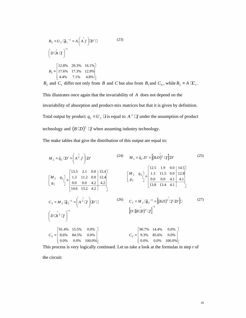
2B and 1C differ not only from B and C but also from 1B and 0C , while 12 CAB ⋅= .

This illustrates once again that the invariability of A does not depend on the

invariability of absorption and product-mix matrices but that it is given by definition.

Total output by product iUq ⋅= 22 is equal to fA ⋅2 under the assumption of product

technology and ( ) fDB ⋅⋅ 2 when assuming industry technology.

The make tables that give the distribution of this output are equal to:

DfADqM ′⋅

=′⋅=

^2

22 .ˆ (24) ( )[ ] DfDBDqM ′⋅⋅=′=

^2

21 ..ˆ (25)

=

2.42.136.142.42.40.00.04.120.02.113.14.150.01.23.13

2

22

gqM

=

1.44.138.131.41.40.00.08.120.05.113.15.140.09.15.12

2

22

gqM

1^2

^21

222 ˆ

−

−

⋅⋅

⋅′⋅

⋅=⋅=

fAD

DfAgMC

(26) ( )[ ]( )[ ]

1^2

^21

222 .ˆ−

−

⋅⋅⋅

⋅′⋅⋅=⋅=

fDBD

DfDBgMC

(27)

=

%0.100%0.0%0.0%0.0%5.84%6.8%0.0%5.15%4.91

2C

=

%0.100%0.0%0.0%0.0%6.85%3.9%0.0%4.14%7.90

2C

This process is very logically continued. Let us take a look at the formulas in step r of

the circuit:

19

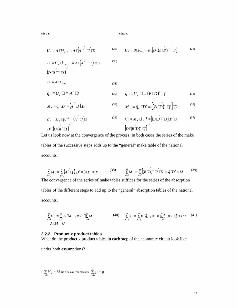
step r:

step r:

( ) DfAAMAU rrr ′⋅⋅⋅=⋅= −−

^1

1 (28) ( )[ ]^

11 fDBDBgBU r

rr ⋅⋅⋅⋅=⋅= −− (29)

( )( )

1^1

^11

1ˆ−

−

−−−

⋅⋅

⋅′⋅⋅⋅=⋅=

fAD

DfAAgUB

r

rrrr

(30)

1−⋅= rr CAB (31)

fAiUq rrr ⋅=⋅= (32) ( ) fDBiUq r

rr ⋅⋅=⋅= (33)

( ) DfADqM rrr ′⋅⋅=′⋅=

^ˆ

(34) ( )[ ] DfDBDqM rrr ′⋅⋅⋅=′⋅=

^

ˆ (35)

( )( )

1^

^1ˆ−

−

⋅⋅⋅′

⋅⋅=⋅=

fADD

fAgMC

r

rrrr

(36) ( )[ ]( )[ ]

1^

^1ˆ−

−

⋅⋅⋅

⋅′⋅⋅⋅=⋅=

fDBD

DfDBgMC

r

rrrr

(37)

Let us look now at the convergence of the process. In both cases the series of the make

tables of the successive steps adds up to the “general” make table of the national

accounts:

( ) MDqDfAMr r

rr =′⋅=∑ ∑ ′⋅⋅=

∞

=

∞

=ˆ

0 0

^ (38) ( )[ ] MDqDfDBM

r r

rr =′⋅=∑ ∑ ′⋅⋅⋅=

∞

=

∞

=ˆ

0 0

^ (39)

The convergence of the series of make tables suffices for the series of the absorption

tables of the different steps to add up to the “general” absorption tables of the national

accounts:

UMA

MAMAUr

rr

rr

r

=⋅=

∑⋅=∑ ⋅=∑∞

=

∞

=−

∞

= 011

1 (40) UgBgBgBU

rr

r rrr =⋅=∑⋅=∑ ∑ ⋅=

∞

=

∞

=

∞

=− ˆˆˆ

01 11

3 (41)

3.2.2. Product x product tables What do the product x product tables in each step of the economic circuit look like

under both assumptions?

3 ∑ =∞

=0rr MM implies automatically ∑ =

∞

=0rr gg .

20

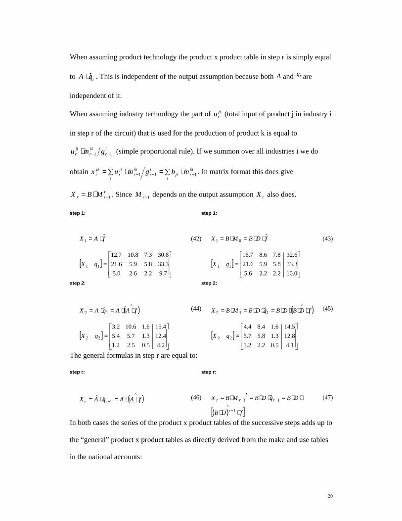
When assuming product technology the product x product table in step r is simply equal

to rqA ˆ⋅ . This is independent of the output assumption because both A and rq are

independent of it.

When assuming industry technology the part of jiru (total input of product j in industry i

in step r of the circuit) that is used for the production of product k is equal to

ir

kir

jir gmu 11 −−⋅ (simple proportional rule). If we summon over all industries i we do

obtain kir

iji

ir

kir

i

jir

jkr mbgmux 111 −−− ⋅∑=⋅∑= . In matrix format this does give

1−′⋅= rr MBX . Since 1−rM depends on the output assumption rX also does.

step 1:

step 1:

fAX ˆ1 ⋅= (42) fDBMBX ˆ

01 ⋅⋅=⋅= (43)

[ ]

=

7.92.26.20.53.338.59.56.218.303.78.107.12

11 qX

[ ]

=

0.102.22.26.53.338.59.56.216.328.76.87.16

11 qX

step 2:

step 2:

( )^12 ˆ fAAqAX ⋅⋅=⋅= (44) ( )^

112 ˆ fDBDBqDBMBX ⋅⋅⋅⋅=⋅⋅=′⋅= (45)

[ ]

=

2.45.05.22.14.123.17.54.54.156.16.102.3

22 qX

[ ]

=

1.45.02.22.18.123.18.57.55.146.14.84.4

22 qX

The general formulas in step r are equal to:

step r:

step r:

( )^1

ˆ fAAqAX rr ⋅⋅=⋅= − (46)

( )[ ]^1

11 ˆ

fDB

DBqDBMBX

r

rrr

⋅⋅

⋅⋅=⋅⋅=′⋅=

−

−−

(47)

In both cases the series of the product x product tables of the successive steps adds up to

the “general” product x product tables as directly derived from the make and use tables

in the national accounts:

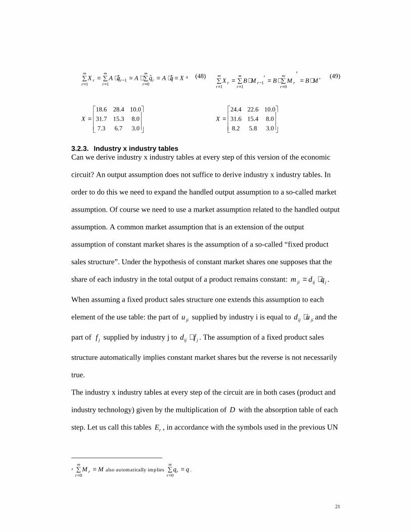
21

XqAqAqAXr

rr r

rr =⋅=∑⋅=∑ ∑ ⋅=∞

=

∞

=

∞

=− ˆˆˆ

01 11

4 (48)MBMBMBX

rr

rr

rr =′⋅=

′∑⋅=∑ ′⋅=∑∞

=

∞

=−

∞

= 011

1

(49)

=

0.37.63.70.83.157.310.104.286.18

X

=

0.38.52.80.84.156.310.106.224.24

X

3.2.3. Industry x industry tables Can we derive industry x industry tables at every step of this version of the economic

circuit? An output assumption does not suffice to derive industry x industry tables. In

order to do this we need to expand the handled output assumption to a so-called market

assumption. Of course we need to use a market assumption related to the handled output

assumption. A common market assumption that is an extension of the output

assumption of constant market shares is the assumption of a so-called “fixed product

sales structure”. Under the hypothesis of constant market shares one supposes that the

share of each industry in the total output of a product remains constant: jijji qdm ⋅= .

When assuming a fixed product sales structure one extends this assumption to each

element of the use table: the part of jiu supplied by industry i is equal to jiij ud ⋅ and the

part of jf supplied by industry j to jij fd ⋅ . The assumption of a fixed product sales

structure automatically implies constant market shares but the reverse is not necessarily

true.

The industry x industry tables at every step of the circuit are in both cases (product and

industry technology) given by the multiplication of D with the absorption table of each

step. Let us call this tables rE , in accordance with the symbols used in the previous UN

4 ∑ =∞

=0rr MM also automatically implies ∑ =

∞

=0rr qq .

22

input-output manual (United Nations, 1973): rr UDE ⋅= . The industry x industry

coefficients are equal to rrr BDgE ⋅=⋅ −−

11ˆ . Since the absorption coefficients matrix

remains constant under the assumption of industry technology the industry x industry

coefficients are equal to BD ⋅ through the whole economic circuit. Under the hypothesis

of product technology they are different in each step since rB is different in each step.

step 1: step 1:

DfADUDE ′⋅⋅⋅=⋅= ˆ11 (50) fBDUDE ˆ

11 ⋅⋅=⋅= (51)

[ ]

=

7.92.20.36.40.342.69.80.191.309.67.105.12

11 gE

[ ]

=

0.102.22.37.43.342.60.91.196.319.68.119.12

11 gE

( )1

1^101

ˆˆBD

fDDfADgUD⋅=

⋅⋅′⋅⋅⋅=⋅⋅−

−

(52) BDgUD ⋅=⋅⋅ −101 ˆ (53)

=⋅

.%4%3.6%2.4%7.13%8.18%3.17%3.15%9.22%3.11

1BD

=⋅

%8.4%7.6%2.4%7.13%1.19%3.17%3.15%1.25%8.11

BD

step 2: step 2:

( ) DfAADUDE ′⋅⋅⋅⋅=⋅=^

22 (54)

( )^122 ˆ

fDBD

BDgBDUDE

⋅⋅⋅

⋅⋅=⋅⋅=⋅=

(55)

[ ]

=

2.45.04.23.12.133.16.63.56.145.12.99.3

22 gE

[ ]

=

1.45.03.23.14.134.16.65.58.135.16.87.3

22 gE

( )

( ) 2

1^

^112 ˆ

BDfAD

DfAADgUD

⋅=⋅⋅

⋅′⋅⋅⋅⋅=⋅⋅−

−

(56) BDgUD ⋅=⋅⋅ −1

12 ˆ (57)

=⋅

%8.4%1.7%4.4%7.13%4.19%5.17%3.15%1.27%8.12

2BD

=⋅

%8.4%7.6%2.4%7.13%1.19%3.17%3.15%1.25%8.11

BD

The general formulas in step r are equal to:

23

step r:

step r:

( ) DfAAUDE rrr ′⋅⋅⋅=⋅= −

^1 (58)

( )[ ]^1

1ˆ

fDBD

BDgBDUDE

r

rrr

⋅⋅⋅

⋅⋅=⋅⋅=⋅=

−

−

(59)

( ) ( ) rrr BDfADDfAA ⋅=⋅⋅⋅′⋅⋅⋅

−−−

1^1

^1 (60) BDgUD rr ⋅=⋅⋅ −

−1

1ˆ (61)

Let us now look at the convergence of the process. Both product and industry

technology, combined with the assumption of a fixed product sales structure, converge

to the same ‘total’ industry x industry table:

∑ ∑ ⋅=∑⋅=⋅=∞

=

∞

=

∞

=1 1 1r r rrrr UDUDUDE (62)

Because in both cases the series of the absorption tables of the different steps add up to

the “general” absorption tables of the national accounts: UUr

r =∑∞

=1.

=⋅

0.30.70.75.89.196.285.91.264.19

UD

Does this mean that the industry x industry table derived under the assumption of a

fixed product sales structure is independent of the technology assumption?

P. Konijn seems convinced this is the case in general with industry by industry tables

(Konijn, 1994). From this he draws the conclusion that industry x industry tables

describe only market relations and are consequently unsuitable for input-output

analysis. They should, according to him, not be used for analysis about the technology

of the economy.

B. Thage of Statistics Denmark also thinks that industry by industry tables do not

involve (strong) technology assumptions but only weaker market assumptions. But from

this he draws the opposite conclusion and prefers industry x industry tables, based on

24

the assumption of a fixed product sales structure as the table which should be published

as part of official statistics together with the supply and use tables.

Is this industry by industry table really independent of technology assumptions? Product

and industry technology converge both to the same industry by industry table in the

“base” version, the table derived from the supply and use tables in national accounts.

But the convergence process is different in both cases. Is the table still independent of

the technology assumption when this is used for input-output analysis? Let us trace this

by means of a very simple example of impact analysis.

3.2.4. Impact Analysis Let us consider a different final demand vector as starting point of the economic circuit

(step 0):

=

6050

150

0q

Under the hypothesis of product technology the output vector q and the product x

product table X that are the outcome of the process engendered by the final demand

vector 0q are only a function of the coefficients matrix A which is assumed to be

constant by definition. The resulting make, absorption and industry x industry tables

also depend on the market shares matrix D .

When assuming industry technology all these tables depend upon both the absorption

coefficients matrix B (assumed to be constant by definition) and the matrix D .

( ) 01 qAIq ⋅−= − (63) ( ) 0

1 qDBIq ⋅⋅−= − (64)

=

2.821.1212.225

q

=

1.829.1203.224

q

25

( )[ ] DqAIDqM ′⋅⋅−=′⋅= −^

01ˆ (65) ( )[ ] DqDBIDqM ′⋅⋅⋅−=′⋅= −

^

01ˆ (66)

=

2.829.1384.2072.822.820.00.01.1210.08.1082.122.2250.00.301.195

gqM

=

1.826.1387.2062.821.820.00.09.1200.07.1082.123.2240.09.294.194

gqM

( )[ ] DqAIAMAU ′⋅⋅−⋅=⋅= −^

01 (67) ( )[ ] 0

^1ˆ qDBIDBgBU ⋅⋅−⋅⋅=⋅= − (68)

=

0.44.98.86.100.244.363.138.371.24

U

=

0.43.98.86.100.243.362.133.378.23

U

( )[ ]^

01ˆ qAIAqAX ⋅−⋅=⋅= − (69) ( )[ ]^

01ˆ qDBIDBqDBX ⋅⋅−⋅⋅=⋅⋅= − (70)

=

0.41.91.96.109.206.393.136.383.23

X

=

0.48.73.106.100.214.392.137.304.30

X

( )[ ] DqAIADUDE ′⋅⋅−⋅⋅=⋅= −^

01 (71) ( )[ ]^

01 qDBIDBDUDE ⋅⋅−⋅⋅⋅=⋅= − (72)

=

0.44.98.83.116.260.366.122.356.24

E

=

0.43.98.83.115.268.355.128.343.24

E

In the base situation we started from given make and use tables (in national accounts)

and calculated:

• the product x product and industry x industry tables belonging to it

respectively under the (technology) assumptions of product and industry

technology and the output assumption of fixed market shares

• the industry x industry tables belonging to it respectively under the

(technology) assumptions of product and industry technology and the

market assumption of a fixed product sales structure

Here we look in first instance which make and absorption tables are generated under

both assumptions given a hypothetical final demand. We notice that the make and

26

absorption tables differ (slightly) according to the technology assumption (the output

assumption is the same in both cases).

The industry by industry tables also differ (slightly) according the technology

assumption. Not only the values but also the coefficients:

( )[ ]( )[ ]

1^

01

^

011ˆ

−−

−−

⋅−⋅

⋅′⋅⋅−⋅⋅=⋅

qAID

DqAIADgE

(73) BDgE ⋅=⋅ −1ˆ (74)

=⋅ −

%8.4%8.6%3.4%7.13%2.19%3.17%3.15%4.25%8.11

ˆ 1gE

=⋅ −

%8.4%7.6%2.4%7.13%1.19%3.17%3.15%1.25%8.11

ˆ 1gE

The coefficients of the industry x industry table based on a fixed product sales structure

remain invariant under the industry technology assumption: they are the same as in the

base situation (national accounts). This is logical since in this case one assumes B to be

constant. Under the assumption of product technology the coefficients of the industry x

industry table based on a fixed product sales structure are variable. This is also logical

because the absorption coefficients matrix B is in general not constant under the

assumption of product technology:

( )[ ] ( )[ ] ( )[ ] ( )[ ]^1

^1

^

01

^

01 fAIDDfAIADqAIDDqAIAD ⋅−⋅⋅′⋅⋅−⋅⋅≠⋅−⋅⋅′⋅⋅−⋅⋅ −−−− (75)

On the basis of this simple exercise we cannot agree with P. Konijn and B. Thage when

they claim that the industry x industry table based on a fixed product sales structure

does not involve technology assumptions.

UD. is the industry x industry table based on a fixed product sales structure regardless

of product or industry technology in the base situation: as an illustrative appendix of

national accounts (although the supposed convergence process to this table is different

in both cases). But when one assumes the coefficients of this table to remain invariable

27

when performing impact analysis (this is what one usually does during input-output

analysis) one combines implicitly the (weaker) market assumption of a fixed product

sales structure with the (strong) assumption of industry technology.

Furthermore because of this we cannot agree with B. Thage when he claims that the (4)

necessary assumptions for carrying out input-output analysis can be assumed to be valid

how matter the input-output table has been constructed (Thage, 2005). Using the

industry x industry table based on a fixed product sales structure for input-output

analysis is implicitly based on the assumption of industry technology. During input-

output analysis this table is related to the product by product table based on industry

technology and constant market shares and we know that this table is in contradiction

with 3 of the necessary assumptions of input-output analysis5.

We have to mention that B. Thage advocates the industry by industry table which is

directly derived from the rectangular supply and use tables (dimension mxn, m

products, n industries, m>n). Only a product by product table based on industry

technology and constant market shares with dimension m x m can be derived from the

rectangular supply and use tables. Product and industry technology can only considered

as counterparts after the supply and use tables are aggregated to square tables with

dimension nxn.

It is not because the m x m product by product table based on industry technology has

no product technology counterpart that the n x n industry by industry table based on a

fixed product sales structure does not involve a technology assumption. The

invariability of its coefficients require the combination of the assumption of a fixed

product sales structure and industry technology but now formulated within the

5 In the working paper published in 1986 the Danish input-output tables were presented as industry by industry tables

based on industry technology (Thage, 1986).

28

framework of the rectangular make and use tables, not the square ones. Look at the

formulas in the right-hand column in this paper and consider the M , U , B and D

matrices to be rectangular: it is then immediately clear that this industry by industry

table is related to the mxm product by product table based on industry technology and

constant market shares when performing input –output analysis.

The product x product table with maximum dimension based on industry technology

and constant market shares makes little sense. The input-structure of products belonging

to the same industry differs only to the degree in which they are produced as a

secondary activity by other industries (Konijn, 1994). Under the assumption of product

technology the identification of a homogeneous branch requires a corresponding

industry in the supply and use tables.

At last we would like mention that the SNA 68 was altogether not that very wrong when

it proposed UD ⋅ as the industry by industry variant of industry technology. This table

is invariant of the technology assumption (and thus solely dependent of the market

assumption of a fixed product sales structure) only when it is considered as an

illustrative appendix to the supply and use tables in the national accounts. But when its

coefficients are used for impact analysis (I guess this is the main reason why input-

output tables are constructed) it is based on the combination of industry technology and

a fixed product sales structure.

3.2.5. Alternative versions of product technology Product technology does not need the assumption of constant market shares to derive

product x product tables with constant coefficients. These coefficients are invariable by

definition. How does product technology perform within the framework of the

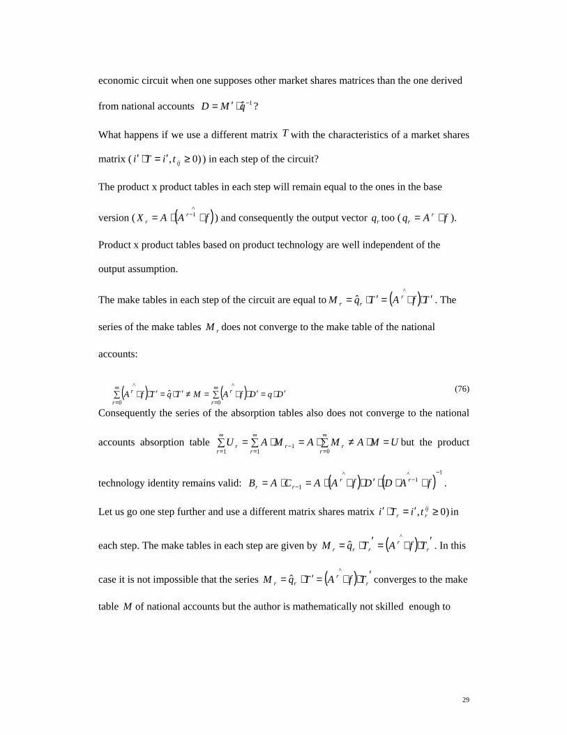
29

economic circuit when one supposes other market shares matrices than the one derived

from national accounts 1ˆ −⋅′= qMD ?

What happens if we use a different matrix T with the characteristics of a market shares

matrix ( )0, ≥′=⋅′ ijtiTi ) in each step of the circuit?

The product x product tables in each step will remain equal to the ones in the base

version ( ( )^1 fAAX r

r ⋅⋅= − ) and consequently the output vector rq too ( fAq rr ⋅= ).

Product x product tables based on product technology are well independent of the

output assumption.

The make tables in each step of the circuit are equal to ( ) TfATqM rrr ′⋅⋅=′⋅=

^ˆ . The

series of the make tables rM does not converge to the make table of the national

accounts:

( ) ( )∑ ′⋅=′⋅⋅=≠′⋅=∑ ′⋅⋅∞

=

∞

= 0

^

0

^ˆ

r

r

r

r DqDfAMTqTfA (76)

Consequently the series of the absorption tables also does not converge to the national

accounts absorption table ∑ ∑ ∑ =⋅≠⋅=⋅=∞

=

∞

=

∞

=−

1 1 01

r r rrrr UMAMAMAU but the product

technology identity remains valid: ( ) ( )1^

1^

1

−−

− ⋅⋅⋅′⋅⋅⋅=⋅= fADDfAACAB rrrr .

Let us go one step further and use a different matrix shares matrix )0, ≥′=⋅′ ijrr tiTi in

each step. The make tables in each step are given by ( ) ′⋅⋅=′⋅= rr

rrr TfATqM^

ˆ . In this

case it is not impossible that the series ( ) ′⋅⋅=′⋅= rr

rr TfATqM^

ˆ converges to the make

table M of national accounts but the author is mathematically not skilled enough to

30

tract to which set of conditions the matrices rT should satisfy in order to realize this

convergence.

3.3. The economic circuit under product technology combined with the output assumption of a constant product-mix

3.3.1. Representation of the economic circuit Imposing the assumption of constant product-mix in the framework of the economic

circuit implies that the output composition each industry remains equal to the

composition in national accounts in every step of the circuit:

CgMC rrr =⋅= −1ˆ (77)The initial effect on output in step 0 is once again equal to final demand by product:

=

4534

123f

This has to be transformed into a make table by means of the product-mix matrix C . A

difference with the assumption of a constant D is that the matrix C cannot transform

f (or rq in general) in a make table with a constant product-mix in one step. This has to

be done in two steps. Firstly final demand by product has to be transformed into final

demand by producing industry:

fCe ⋅= −1 (78)

=

0.456.354.121

e

1−C has only to be used to calculate the column totals of the make table in each step,

not the individual elements. For this the matrix C is used in a second phase:

( )^1

0 ˆ fCCeCM ⋅⋅=⋅= − (79)

31

=

0.456.354.1210.450.450.00.00.340.04.276.60.1230.02.88.114

0

00

gqM

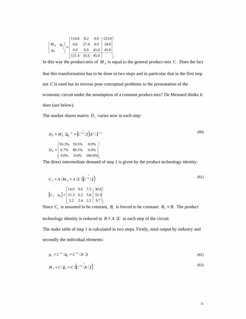
In this way the product-mix of 0M is equal to the general product-mix C . Does the fact

that this transformation has to be done in two steps and in particular that in the first step

not C is used but its inverse pose conceptual problems to the presentation of the

economic circuit under the assumption of a constant product-mix? De Mesnard thinks it

does (see below).

The market shares matrix rD varies now in each step:

( ) 1^11

000ˆˆ −−− ⋅′⋅⋅=⋅′= fCfCqMD (80)

=

%0.100%0.0%0.0%0.0%5.80%7.6%0.0%5.19%3.93

0D

The direct intermediate demand of step 1 is given by the product technology identity:

( )^1

01 fCCAMAU ⋅⋅⋅=⋅= − (81)

[ ]

=

7.92.24.22.53.338.52.63.218.303.76.90.14

11 qU

Since rC is assumed to be constant, rB is forced to be constant: BB =1 . The product

technology identity is reduced to CAB ⋅= in each step of the circuit.

The make table of step 1 is calculated in two steps. Firstly, total output by industry and

secondly the individual elements:

fACqCg ⋅⋅=⋅= −− 11

11 (82)

( )^1

11 ˆ fACCgCM ⋅⋅⋅=⋅= − (83)

32

=

7.97.414.227.97.90.00.03.330.01.322.18.300.06.92.21

1

11

gqM

The corresponding market shares matrix 1D clearly differs from 0D and D :

( ) ( )1^^

11111 ˆ

−−− ⋅⋅′⋅⋅⋅=⋅′= fACfACqMD (84)

=

%0.100%0.0%0.0%0.0%9.89%3.13%0.0%1.10%7.86

1D

Let us now proceed with step 2:

( )^1

12 fACCAMAU ⋅⋅⋅⋅=⋅= − (85)

[ ]

=

2.45.08.20.14.123.12.79.34.156.12.116.2

22 qU

fACqCg ⋅⋅=⋅= −− 212

12 (86)

( )^21

22 ˆ fACCgCM ⋅⋅⋅=⋅= − (87)

=

2.42.155.122.42.40.00.04.120.07.117.04.150.05.39.11

2

22

gqM

( ) ( )1^

2^

211222 ˆ

−−− ⋅⋅′⋅⋅⋅=⋅′= fACfACqMD

(88)

=

%0.100%0.0%0.0%0.0%5.94%9.22%0.0%5.5%1.77

2D

The general formulas in step r are equal to:

( )^11

1 fACCAMAU rrr ⋅⋅⋅⋅=⋅= −−− (89)

fACqCg rrr ⋅⋅=⋅= −− 11 (90)

( )^1ˆ fACCgCM r

rr ⋅⋅⋅=⋅= − (91)

33

( ) ( )1^^

11ˆ−

−− ⋅⋅′⋅⋅⋅=⋅′= fACfACqMD rrrrr

(92)

Let us look now at the convergence of the process:

( ) ( ) MgCqCCfACCMr r

rr =⋅=⋅⋅=∑ ∑ ⋅⋅⋅= −∞

=

∞

=

− ˆ^1

0 0

^1 (93)

The series of the make tables of the successive steps adds up to the “general” make table

of the national accounts. This automatically implies that the series of the absorption

tables of the different steps to add up to the “general” absorption tables of the national

accounts: ∑ =⋅=∑ ⋅=∞

=

∞

=−

1 11

r rr UMAMAUr .

Notice that this version of the economic circuit can also be considered as a particular

case of the economic circuit with differing market share matrices

( ) ( )1^^

1−

− ⋅⋅′⋅⋅⋅= fACfACT rrr . The convergence of series of the make tables of the

successive steps adds up to the “general” make table of the national accounts can also

be seen from a different angle:

( ) ( ) ( ) ( ) ( ) MfACCfACfACfATfAr

rrr

rrr

r

r =∑ ⋅⋅⋅=

′

⋅⋅′⋅⋅⋅⋅∑ ⋅=′⋅∑ ⋅

∞

=

−−

−∞

=

∞

= 0

^1

1^^1

0

^

0

^

(94)

3.3.2. Product by product and industry by industry tables Regarding product by product tables, since these are independent of the output

assumption when supposing product technology, the formulas are the same as given in

the left-hand columns of page 20 and 21.

How do we have to derive industry x industry tables in each step of this version of the

economic circuit? Once again we need to expand the handled output assumption to a so

called market assumption. Just like in the case of constant market shares we need to use

a market assumption related to the handled output assumption. A common market

assumption that is an extension of the output assumption of a constant product-mix is

34

the assumption of a so called “fixed industry sales structure”. Under the hypothesis of a

constant product-mix one supposes that the share of each product in the total output of

an industry remains constant: ijiji gcm ⋅= . When assuming a fixed industry sales

structure one extends this assumption to each element of the industry by industry table:

the part of product j in liE is equal to lijl Ec ⋅ and the part of je taken in by product j is

equal to ljl ec ⋅ . The assumption of a fixed industry sales structure automatically implies

a constant product-mix but the reverse is not necessarily true.

This means that: ∑ ⋅=l

lijlji Ecu what is equal to ECU ⋅= or UCE ⋅= −1 .

The industry x industry tables in each step of the circuit are then given by the

multiplication of 1−C with the absorption table of each step: rr UCE ⋅= −1 . The industry

x industry coefficients are equal to 11ˆ −

−⋅ rr gE . Since the absorption coefficients matrix is

forced to remain constant because A (product technology) and C (fixed industry sales

structure) the industry x industry coefficients are equal to BC ⋅−1 through the whole

economic circuit.

step 1:

( )^11

11

1 fCCACUCE ⋅⋅⋅⋅=⋅= −−− (95)

[ ]

=

7.92.24.22.57.411.74.72.274.229.53.82.8

11 gE

( ) ( ) BCfCfCCACgE ⋅=⋅⋅⋅⋅⋅⋅=⋅ −−

−−−− 11^

1^111

01 ˆ (96)

=⋅−

%8.4%7.6%2.4%8.15%8.20%4.22%2.13%4.23%7.6

1 BC

35

step 2:

( )^11

21

2 fACCACUCE ⋅⋅⋅⋅⋅=⋅= −−− (97)

[ ]

=

2.45.08.20.12.155.17.80.55.123.18.95.1

22 gE

( ) ( ) BCfACfACCACgE ⋅=⋅⋅⋅⋅⋅⋅⋅⋅=⋅ −−

−−−− 11^

1^

11101 ˆ

(98)

Let us now look at the convergence of the process. The convergence of the series of the

industry by industry tables of each step to the ‘total’ industry x industry table is self-

evident:

∑ ∑ ⋅=⋅=⋅=∑∞

=

∞

=

−−−∞

= 1 1

111

1 r rrr

rr UCUCUCM (99)

The SNA 68 described the table UC ⋅−1 as the industry by industry variant of product

technology. This was exaggerated but not entirely wrong. It is (among o. things, see

below) the combination of product technology and a fixed industry sales structure.

We observe this if we perform again the impact analysis described on page 24-28 but

now based on the combined assumptions of product technology and a fixed industry

sales structure.

The total output product remains independent of the output assumption (product

technology):

( ) 01 qAIq ⋅−= − (100)

=

2.821.1212.225

q

The total output by industry can consequently be derived:

( ) 011 qAIqCg ⋅−=⋅= −− (101)

36

=

2.820.1433.203

g

The make table is calculated on the assumption of a constant product-mix:

( )[ ]^

011ˆ qAICCgCM ⋅−⋅⋅=⋅= −− (102)

=

2.820.1433.2032.822.820.00.01.1210.00.1101.112.2250.00.332.192

gqM

Finally the absorption table can be derived by the product technology identity:

( )[ ]^

011 qAICCAMAU ⋅−⋅⋅⋅=⋅= −− (103)

=

0.46.96.86.107.247.353.135.384.23

U

The industry by industry tables are derived as:

( )[ ]^

01111 qAICCACUCE ⋅−⋅⋅⋅⋅=⋅= −−−− (104)

=

0.46.96.80.138.295.458.104.337.13

E

The industry by industry coefficients have remained equal to BC ⋅−1 :

( )[ ] ( )[ ]1^

011

^

01111ˆ

−−−−−−− ⋅−⋅⋅⋅−⋅⋅⋅⋅=⋅ qAICqAICCACgE

(105)

This is very logical because the two matrices that form the matrix product are assumed

to be constant: C by definition and the invariability of B follows from the combined

invariability of C and A (by definition).

37

3.3.3. Industry technology and a constant product-mix Combining product technology with a constant product-mix forces the absorption

coefficients matrix B to be constant. Industry technology means that the B matrix is

constant by definition. Is there then still any difference between product and industry

technology when they are both combined with the output assumption of a product-mix

or the related market assumption of a fixed industry sales structure?

Hardly: all the make, use and industry by tables are equal in every step of the circuit and

consequently the total tables too, as well as in the base situation of the national accounts

as when performing input-output analysis. Only the product by product tables differ and

under the hypothesis of industry technology and they have now variable technical

coefficients:

step 1:

fDBMBX ˆ001 ⋅⋅=′⋅= (106)

[ ]

=

7.92.21.24.53.338.59.56.218.303.71.84.15

11 qX

The coefficients are clearly different from DB ⋅ :

01

0ˆ DBfMB ⋅=⋅′⋅ − (107)

=⋅

%8.4%2.6%4.4%9.12%4.17%6.17%1.16%9.23%5.12

0DB

step 2:

( )^1

11112 ˆ fCBDBqDBMBX ⋅⋅⋅⋅=⋅⋅=′⋅= − (108)

[ ]

=

2.45.02.25.14.123.18.54.54.156.18.80.5

22 qX

38

11

11 ˆ DBqMB ⋅=⋅′⋅ − (109)

=⋅

%8.4%6.6%0.5%9.12%3.17%5.17%1.16%4.26%3.16

1DB

The general formulas in step r are equal to:

( )^

111111 ˆ

⋅⋅⋅⋅=⋅⋅=′⋅=

−−−−−− fCBDBqDBMBX r

rrrrr (110)

11

11 ˆ −−

−− ⋅=⋅′⋅ rrr DBqMB (111)The series of these product by product tables in each step converges to the same total

product by table as under the combined assumptions of product technology and constant

market shares:

qDBMBMBXr r

rr ˆ1 1

1 ⋅⋅=′⋅=∑ ∑ ′⋅=∞

=

∞

== (112)

But when we perform again the same impact analysis we obtain a product by product

table with different technical coefficients. This illustrates that this version of industry

technology has no stable product by product coefficients.

( ) CqCBCIBCgBMBX ′⋅

⋅⋅⋅−⋅=′⋅⋅=′⋅= −−−

^

0111ˆ

(113)

=

0.49.74.106.100.215.393.139.300.31

X

( ) ( )^

0111

^

011111 ˆˆ

⋅⋅⋅−⋅⋅′⋅

⋅⋅⋅−⋅=⋅′⋅=⋅ −−−−−−−− qCBCICCqCBCIBqMBqX

(114)

=⋅

%8.4%5.6%6.4%9.12%3.17%5.17%1.16%5.25%8.13

DB

Finally we like to close this part with the remark that the industry x industry table

UC ⋅−1 is also the combination of industry technology and a fixed industry sales

structure.

39

3.4. An attempt to understand Mesnard’s critique As a starting-point we would like to repeat that de Mesnard’s identifies product

technology with the invariability of the B and C matrices. Consequently we can

suppose that his critique is solely directed against this variant of product technology.

According to the de Mesnard the beginning of the economic circuit with the

transformation of final demand by product into final demand by industrial output

fCe ⋅= −1 (and in general the transformation rr qCg ⋅= −1 ) is an illegal transformation.

Only the transformation rr gCq ⋅= remains true. We try to follow him here but we

cannot follow him anymore when he illustrates his statement with an (although

incomplete) example (at last).

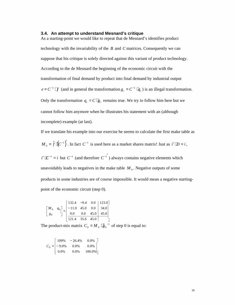
If we translate his example into our exercise he seems to calculate the first make table as

( )′⋅= −10

ˆ CfM . In fact 1−C is used here as a market shares matrix! Just as iDi =⋅′ ,

iCi =⋅′ −1 but 1−C (and therefore ′−1C ) always contains negative elements which

unavoidably leads to negatives in the make table 0M . Negative outputs of some

products in some industries are of course impossible. It would mean a negative starting-

point of the economic circuit (step 0).

−

−

=

0.456.354.1210.450.450.00.00.340.00.450.110.1230.04.94.132

0

00

gqM

The product-mix matrix 1000 ˆ −⋅= gMC of step 0 is equal to:

−

−=

%0.100%0.0%0.0%0.0%0.0%0.9%0.0%4.26%109

0C

40

This is clearly not equal to the product-mix matrix C . The use of 1−C as a (wrong)

market shares matrix does not guarantee the invariability of the product-mix coefficient

matrix.

Continuing with step 1:

( )′⋅⋅=⋅= −101

ˆ CfAMAU (115)

[ ]

=

7.92.20.35.43.338.51.64.218.303.74.132.10

11 qU

( ) ( )1^

111011

ˆˆ−

−−− ⋅⋅′

⋅⋅=⋅= fCCfAgUB (116)

=

%8.4%5.8%7.3%9.12%1.17%6.17%1.16%6.37%4.8

1B

The actual absorption coefficients matrix of step 1 also differs from the general matrix

B . The identity 01 CAB ⋅= remains valid.

Just as 0M , the make table of step 1 ( ) ( ) ( )′⋅⋅=′⋅= −− 1^

111 ˆ CfACqM contains negative

elements, which is not allowed:

−

−

=

7.91.444.227.97.90.00.03.330.01.448.108.300.04.22.33

1

11

gqM

( ) ( ) ( ) 111^1111 ˆ −−−− ⋅⋅⋅

′⋅⋅=⋅= fACCfAgMC (117)

−

−=

%0.100%0.0%0.0%0.0%6.105%0.48%0.0%6.5%0.148

1C

1C differs clearly from C but also from 0C .

Let us now continue with step 2.

41

( ) ( )′⋅⋅⋅=⋅= −1^12 CfAAMAU (118)

[ ]

=

2.45.02.35.04.123.12.70.44.156.18.130.0

22 qU

( ) ( ) ( )1^

11^1122 ˆ

−−−− ⋅⋅⋅

′⋅⋅⋅=⋅= fACCfAAgUB

(119)

=

%8..4%7.7%4.2%9.12%2.17%8.17%1.16%1.33%0.0

2B

12 CAB ⋅= (120)

( ) ( ) ( )′⋅⋅=′

⋅= −− 1^

2122 ˆ CfACqM (121)

−

−

=

2.42.155.122.42.40.00.04.120.04.160.44.150.02.16.16

2

22

gqM

( ) ( ) ( )1^

11^

21222 ˆ

−−−− ⋅⋅⋅

′⋅⋅=⋅= fACCfAgMC

(122)

−

−=

%0.100%0.0%0.0%0.0%0.107%0.32%0.0%7.7%0.132

2C

In general ( ) ( ) ( )1^

111^1

−−−−− ⋅⋅⋅′⋅⋅⋅= fACCfAAB rr

r and

( ) ( ) ( )1^

11^ −

−− ⋅⋅⋅′⋅⋅= fACCfAC rrr will differ from B and C in every step of the

circuit. Is this not contrary to de Mesnard’s adherence to the assumption of constant

absorption and product-mix coefficients as the definition product-technology? The

make tables ( ) ( )′⋅⋅= −1^

CfAM rr will always contain negative elements.

Moreover the series of the make tables rM in such a version of the economic circuit

does not converge to the make table of the national accounts:

42

( ) ( ) ( ) ( ) DqDfAMCqCfAr

r

r

r ′⋅=′⋅∑ ⋅=≠′

⋅=′

⋅∑ ⋅∞

=

−−∞

=ˆˆ

0

^11

0

^ (123)

But we really do not see what the negative elements of rM in the example above have

to do with the negatives that are currently mentioned in association with product

technology. I think I demonstrated a correct version of the economic circuit under

product technology where the make table is non-negative in every step since D is non-

negative. The negatives that possibly arise, when applying product technology to derive

product x product tables from make and absorption tables, are not those in 1−C , which

are inevitable, but the ones in 1−⋅= CBA , which are in theory evitable, since the

absence or presence of negatives in 1−⋅ CB is conditional (Konijn 1994, Steenge, 1989

and 1990).

These are negative inputs that arise during the transformation of B into A when an

industry does not register certain inputs in such a measure as it should do according the

product technology assumption. If it does register these inputs (as in our example) these

negatives simply never appear. Moreover I have the impression that the matrices rM in

the example above exhibit negative unconditional outputs. Is this not a complete

different matter?

What surprises us the most is that in the example given by the De Mesnard the product-

mix is obviously not constant while he initially associates product technology with a

constant product-mix.

As a conclusion we would like to say that we have serious considerations on de

Mesnard’s critique of product technology:

• he defines product technology as the exhibition of a constant product-mix. Is his

critique only valid against this special case of product (or industry!) technology

43

combined with a constant product-mix? What remains of his critique if one

accepts the more general definition of product technology?

• if one considers his critique as only directed against the assumption of an

invariable product-mix why is this one not constant in the example he gives to

illustrate his statement? Is he here not in contradiction with his own starting-

point?

44

4. Practical Aspects

4.1. Integration in National Accounts We know now that input-output tables are never entirely integrated in national accounts.

They are always explicitly (product by product tables) or implicitly (industry by

industry) based on simple but far-reaching modelling assumptions (strong technology

assumptions). They are still closely related to the underlying supply and use tables and

basic data but there is a “modelling cut”.

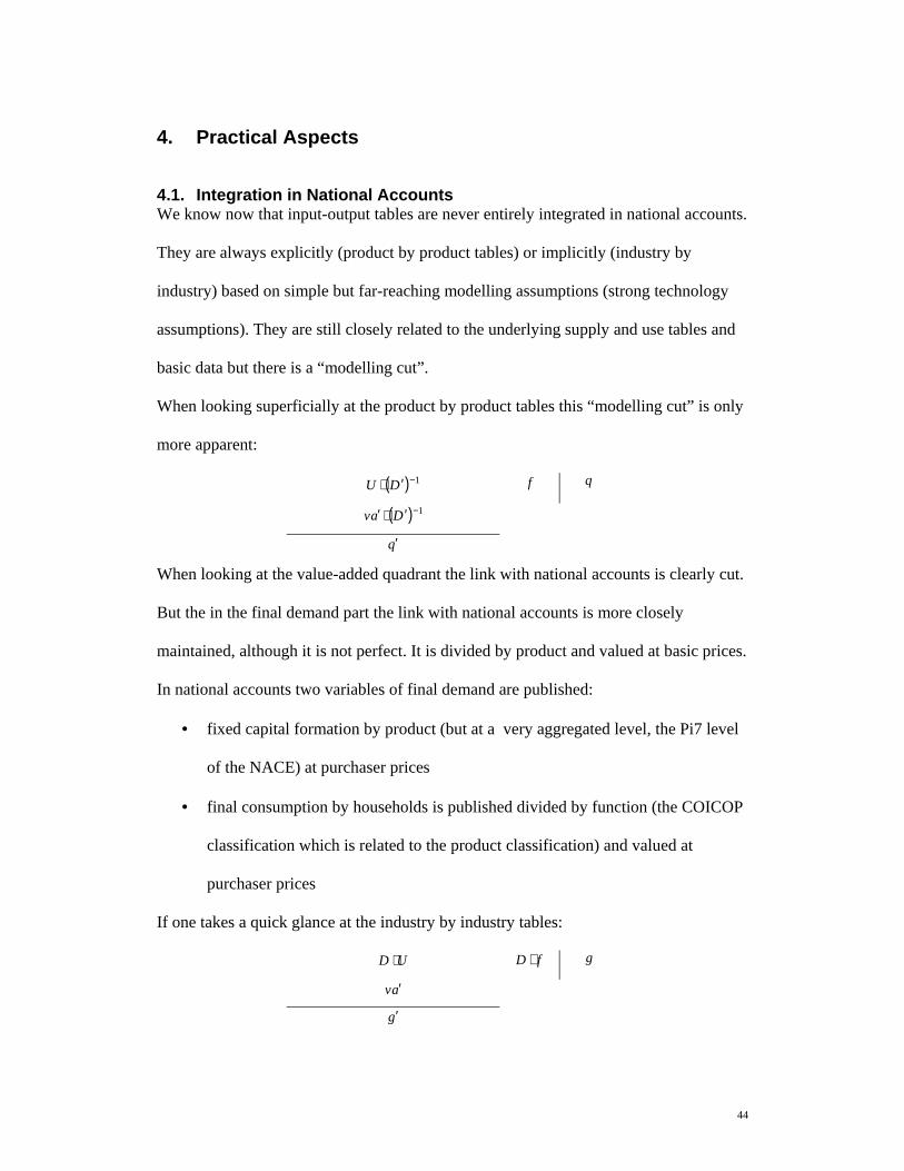
When looking superficially at the product by product tables this “modelling cut” is only

more apparent:

( ) 1−′⋅ DU f q

( ) 1−′⋅′ Dav

q′

When looking at the value-added quadrant the link with national accounts is clearly cut.

But the in the final demand part the link with national accounts is more closely

maintained, although it is not perfect. It is divided by product and valued at basic prices.

In national accounts two variables of final demand are published:

• fixed capital formation by product (but at a very aggregated level, the Pi7 level

of the NACE) at purchaser prices

• final consumption by households is published divided by function (the COICOP

classification which is related to the product classification) and valued at

purchaser prices

If one takes a quick glance at the industry by industry tables:

UD ⋅ fD ⋅ g

av ′

g′

45

Value added ( av ′ ), total output ( g ) and consequently total intermediate consumption

are published in the national accounts by industry. Here the link with the national

accounts is perfectly maintained. But final demand is now given by industry ( fD ⋅ )

while in the national accounts it is published by product or by function (which is related

to products not to industries). Here the link with national accounts is clearly cut.

4.2. The statistical unit and the degree of secondary production Different types of statistical units are considered in official guidelines: the enterprise,

the local unit, the kind-of-activity unit (KAU) and the local kind-of-activity unit (local

KAU) or establishment as it is called in the SNA.

This last one is the recommended unit. The present Belgian statistical apparatus has no

experience with this concept because the enterprise is the statistical unit6 with the

consequence that the supply and use tables are very heterogeneous.

The definition of the local KAU or establishment given in the SNA or ESA is very

abstract. The ESA defines it as “the part of a KAU which corresponds to a local unit.

The KAU groups all parts of an institutional unit in its capacity as producer contributing

to the performance of an activity at class level (4 digits) of the NACE rev. 1 and

corresponds to one or more operational subdivisions of the institutional unit. The

institutional unit’s information system must be capable of indicating or calculating for

each local KAU at least the value of production, intermediate consumption,

compensation of employees, the operating surplus and employment and gross fixed

capital formation” (Eurostat, 1995)

6 Before the introduction of the ESA 95 the local unit was the statistical unit of the industrial branches only. There was

no systematical statistical interrogation of the service industries (Avonds and Gilot, 2002)

46

According to me (by intuition) this means that when an enterprise surpasses a certain

size and its secondary production(s) a certain threshold it has to be split up into several

KAU’s or local KAU’s (when it has several local units).

The SNA adds the types of employees and hours worked and the stock of capital and

land used to the minimum data requirements. Notice that intermediate consumption is

not required by product. If only total intermediate consumption is known at the level of

the (local) KAU when intermediate consumption by product is known at the level of the

enterprise how are the latter attributed the to (local) KAU’s? We suppose that in this

case clearly some modelling at the micro-level should be done. Is this done according to

the industry technology assumption (purely proportional according to the outputs of the

local KAU’s) or closer to the product technology principle when inputs are attributed

according to the generally known input structure of the products corresponding with the

(nearly homogeneous) outputs of the (local) KAU’s?

Some caution is certainly recommended when comparing input-output tables that are

compiled on the basis of different statistical units.

Product by product tables remain in theory perfectly comparable because they are

directed towards the same result: the input structure and output of homogeneous

branches. The type of statistical unit will off course in practice affect to a certain degree

the outcome.

When comparing industry by industry tables based on different statistical units this is

not the case because these tables reproduce transactions between enterprises, local units,

KAU’s or local KAU’s according to the type of statistical unit.

Regarding secondary production B. Thage declares “The observed extent of secondary

production does therefore not posses any observable characteristics of its own. The

47

elusive character of the concept of secondary production makes it difficult to justify that

it should be of particular interest statistically just because it is produced in two or more

industries at a certain level of industry or product aggregation” (Thage, 2005).

We have to reply by repeating that input-output analysis is based on homogeneous

branches (homogeneous within the dimensions of the input-output table). Secondary

production remains the essential difference between supply and use tables on the one

hand and homogeneous input-output tables on the other. The degree of secondary

production should be considered at the level of the working format of the supply and

use tables and the input-output table should be compiled at the maximum (square)

dimension because in this case the relation with the statistical data is diminishes less

and more applications are feasible and accurate.

When the supply and use tables are compiled on the basis of (local) KAU’s they are

already very homogeneous and the use table approaches the product by product table

(for a very good reason). B. Thage mentions the registration of secondary production

only for manufacturing industry and the assumption of the service industries as being

homogeneous (even at the level of the enterprises) by lack of statistical data. In this case

the use table resembles even more to a product by product table but now for a bad

reason. Further he makes mention of agriculture, trade and construction as already being

constructed as homogeneous branches in the supply and use tables. Honestly, I really

ask myself if one can still speak of industry by industry tables in such a case. If the

industries in the supply and use tables are already rather (or in many cases already

completely) homogeneous the ”industry by industry” table can be more or less

identified with a Leontief table (Konijn, 1994) but can it still be considered as an

industry by industry table?

48

In Belgium we do not have the (local) KAU as statistical unit and trade and construction

are registered as heterogeneous industries in the supply and use tables in order to

maintain the link with the business register. But we do have data on the output

composition of the service industries (at the enterprise level). If we look at the degree of

secondary production of the service industries, the assumption of their homogeneity (at

the enterprise level) does not seem acceptable, at least for the so-called business-

services (NACE 65 up to and including 74).

Table 1: The degree of secondary production presented at the level of the P6 and A6 classifications for Belgium

These are not the “official” Belgian input-output tables but constant price tables

calculated for the EUKLEMS project with the disaggregations of certain industries and

one product, all corresponding with the national accounts version 2005 (Avonds et al.,

2007). The official tables correspond with different versions of the national accounts

and do only exist at current prices. Moreover, the “official” tables for 1996 and 1998

have never been calculated7.

The table does not reflect the heterogeneity of 6x6 tables but of the square tables at

maximum level8. The ratio of total secondary output to total output (the ratio of total

off-diagonal elements to total elements in the make tables) is used as a criterion. This

ratio is very high and fluctuates between 16% and 18%. Regarding the degree of

secondary production at the level of the (mega) industries we observe a break between

1999 and 2000.We do fear that the (official) tables for 1997 and 1999 are (partially)

calculated as an extrapolation of the 1995 table notwithstanding the fact that the

statistical data are yearly available.

7 We have to admit that the tables for 1996 and 1998 are a retro- and extrapolation of the tables for 1997. 8 1995: 159 x 159, 2000: 152 x 152, other years: 137 x 137.

49

From 2000 on the degree of heterogeneity of the business services is equal to 15% or

16%. Compared to 1995 the pattern of secondary production does not really change

qualitatively (no disappearance of certain secondary production and the appearance of

new ones), the share of the existent secondary production has increased.

• Banks do have a large secondary production of supporting services of financial

institutions. The insurance companies have large secondary activities in real

estate services (CPA 70) and business services (CPA 74)

• The real estate services do have a considerable secondary output of construction

activities (CPA 45)9

• The set of industries belonging to the NACE Division 74 “Other Business

Services” do form a cluster. The largest part of the secondary output is always

secondary output characteristic of other industries belonging to Division 74.

Further there are also secondary activities of computer services (CPA 72)10 and

waste collection and treatment (CPA 90). At last there is an industry of the

“other “category within this division that has a whole series of rather small

secondary productions of manufacturing goods which all counted together are

significant, comparable to the wholesale trade industry (if the statistical unit is

the local KAU this activity is normally moved the manufacturing industries, the

PRODCOM statistic has a low threshold)

• The whole of other services (NACE 75 up to and including 95) has a small but

gradually increasing degree of secondary production. The significant secondary

outputs are the incidental sales of government (an ESA 79 concept: Eurostat,

9 Here is taken care of when construction is already a homogeneous branch in the supply and use tables. 10 I am talking here of market computer services and not output for own final use.

50

1979) and production of market services by the non-market service industries

that are the market variant of their characteristic production.

4.3. The distinction between the use of domestic output and imports In general the use table for imports is calculated by assuming constant import ratio’s (a

simple proportional distribution of imports over each row of the use table), which is

similar to the assumption of a fixed product sales structure. According to B. Thage this

is contradictory with the separation of the input-output table into input-output tables for

domestic output and imports when assuming product technology.

We think this is only the case when one assumes that the input structure of a product is

the same in every industry where it is produced but also that the ratio of

domestic/imported for all the intermediary used goods and services for the making of

this product is the same in all these industries.

The non-published input-output manual of Eurostat (Eurostat, 2002) proposed a method

to avoid this. This method is based on the product technology model, linked to the

hypothesis that inside one industry the ratio use of imports/total use of intermediate

products is the same for the principal and secondary activities. This means that the

technical coefficients are unique for a product no matter in which industry it is produced

as principal or secondary output, but the composition in the technical coefficients of

domestic output and imports can vary according to the industry.

In Belgium about 70% of the imports of goods are exogenously attributed on the basis

of foreign trade data (Van den Cruyce, 2002, 2003 and 2004). This information is

maintained when calculating the input-output table for imports.

51

4.4. Negatives and redefinitions A serious difficulty encountered during the application of product technology are

negatives in the matrix product 1−⋅ MU or 1−⋅CB . This means that an industry does not

use enough (or at all) the inputs it is supposed to use for its secondary production. These

negatives can have different reasons: errors in basic data or in the compilation of make

and use tables (they can be traced and corrected), heterogeneity of the industry

classification, ...

This last phenomenon is often indicated as a possible cause of negatives when applying

the product technology model (Gigantes, 1970, Konijn 1994, Rainer and Richter, 1992,

Stone et al., 1963): when calculating the input structures of products (homogeneous

branches) these are aggregated to the level of the industry classification these

aggregated to the level of the industry classification. At this level the principal

production of an industry is an aggregation of different original products for which the

production processes (inputs) may differ in reality. The input structure of a

homogeneous branch is largely determined by the input structure of the primary

producer. This means that the input structure of a homogeneous branch is more or less a

weighted average of the input structures of the products made by the primary producer.

Another industry can produce, as a secondary activity, only some of these original

products or in another composition than the primary producer. But this is not taken into

account in the transformation matrix of the product technology model. It is assumed

here that secondary producers have the same composition as the main one. If this is not

the case negatives can be created in the input-output model. A disaggregation of the

primary industry can be useful to handle this kind of problem.

If the product technology assumption is not (entirely) valid or if it is not possible to

realize the aimed disaggregations in practice (if the industries would have to broken up

52

into an impossible number of activities) “redefinitions” can be carried out. A

redefinition is the manual transfer of the inputs of a part of the secondary production of

an industry whereby these inputs are estimated exogenously so that that no negatives

appear after the transformation. This does not necessarily mean that one rejects entirely

the product technology model in favour of the industry technology model. If the input-

structure of the manual transformation is similar to the one of the primary producer one

remains much closer to product technology than industry technology. If one takes the

use table after redefinition as the new use table the mathematical properties of the

product technology model remain valid.

During the compilation of the Belgian input-output tables for 1995 and 2000

redefinitions were made under the denomination of “analytical disaggregations”

(Avonds and Gilot, 2002, Avonds, 2002 and 2005). The “activity technology model”

developed by Konijn does start as a redefinition. The inputs of activities for which no

primary producer (industries) exists are estimated exogenously. After that the activity

technology model goes one step further: the outputs of these activities are distinguished

as separate products. This means that extra products are introduced in the input-output

system of which the uses should be distinguished in the use table. In this way, the

conditions of the Leontief input-output model (homogeneous branches) are once again

met (Konijn, 1994). The US Bureau of Economic Analysis (BEA) applied a

“redefinition process” of which they declared that it is similar to product technology as

a first step in the transformation of supply and use tables into the “benchmark” input-

output tables. The second step consists of the application of the industry technology

principle (Guo et al., 2002). A more overall type of redefinition is the application of

specific transformation matrices to each row (product) of the absorption table, avoiding

53

in this way the emergence of negatives, instead of one general transformation matrix

( ) 1−′D (Reich et al., 1989, Stahmer, 1985).

Small negatives can be corrected by putting them equal to zero and rebalancing the

input-output table with the RAS method or applying the Almon algorithm to the

absorption table (a mathematical iterative method not entirely equal to but still based on

the product technology assumption, Almon, 1970, 1998 and 2000). After applying such

mechanical procedures the mathematical properties of the product technology model are

not entirely valid anymore and the input-output table does slightly disobeys the 4

assumptions of input-output analysis. In this case one has made an approach of an input-

output table meeting these 4 assumptions.

B. Thage also mentions redefinitions in the last part of his paper. He considers manual

splitting up of KAU’s when no information is available and they span more than one

heading at the first level of the industrial classification (for example the A6 version of

the NACE)11. This is a redefinition that remains within the framework of the supply and

use tables. It is also modelling at he micro-level, where have to make the same remark

as on page 46. He limits himself to the statement that these redefinitions are “made at

hand based on the best available information and judgement of the national

accountants”. I think one can hardly disagree that when an industry combines

productions belonging to the first level of break-down of an industry classification (for

example manufacturing and wholesale) the implausibility of the industry technology

assumption is obvious. Applying industry technology explicitly or implicitly does not

make sense in such a case. These redefinitions can remain within the framework of the

supply and use tables or executed only during the transformation into the input-output

11 The SNA 93 recommends this for vertically integrated enterprises (United Nations et al., 1993). The vertical

integration of enterprises is a typical cause of negatives during the application of product technology.

54

tables. According to him these redefinitions are quit different from the product

technology model because:

• only part of secondary production is redefined

• they are not (pure) mathematical procedures

• no negatives appear

Of course we agree that redefinitions are different from the pure mathematical version

of the product technology model but we think that they are still related to it. Large

secondary productions causing large negatives are in general not mathematically

transferred and subsequently mechanically corrected but treated with redefinition type

transfers (where the product technology principle is mitigated) as explained above.

When input-output tables are calculated by a combination of redefinitions and explicit

or implicit application of industry technology (industry by industry tables based on a

fixed product sales structure) one applies in reality a mixed technology model: a

combination of (a mitigated version of) product technology and industry technology as

was declared in the BEA paper.

Moreover if industry by industry tables would be independent of technology why bother

to make them more homogeneous by means of these redefinitions (and even to

introduce less heterogeneous statistical units than the enterprise)? Would it still matter?

If it matters does this not mean that one wants these tables to resemble more to a

Leontief table (a table based on homogeneous branches obeying the axioms of input-

output analysis) than a industry by industry table without these interventions and that

one is (maybe implicitly or unconsciously) considering technology assumptions?

55

Conclusions

Input-output tables are never fully integrated into national accounts in the sense that

they are always based on far-reaching modelling assumptions, even when these

assumptions are very simple. Product by product tables are based on a combination of

technology assumptions (the input structure of products and consequently of the

industries producing them) and output assumptions (the output composition of

industries in terms of products). The industry by industry tables are not only based on

market assumptions (the share of deliveries by industries in the final and intermediate

use of each product) but also on technology assumptions. The only tables that are really

integrated in the national accounts are the supply and use tables from which the input-

output tables are derived as models.

Products by product tables based on the product technology assumption have stable

coefficients by definition. A certain flexibility in the choice of the output assumption

exists here. One simply has to make an output assumption that does not lead to

unconditional negatives in the make table and guarantees convergence in terms of the

economic circuit. It is on the base of these findings that we have serious considerations

with the critique formulated against the product technology model by de Mesnard.

Firstly his critique does not seem directed against the product technology model in

general but against the output assumption of a constant product-mix (which he identifies

with product technology). Secondly in the example in which he illustrates his statement

the product-mix is variable (and impossible). I cannot dispose myself of the impression

that he is contradicting himself here.

56

Because all of this I continue to be inclined to think that product by product tables based

on product technology remain the only tables that obey the axioms on which input-

output analysis is based.

Considering B. Thage’s arguments in favour of the industry by industry table based on

the market assumption of a fixed product sales structure there is only one that is

completely indisputable. It is indeed (much) easier to derive such a table from the

supply and use tables than to compile homogeneous tables based on product technology.

How much easier this is depends on the degree of secondary production in the supply

and use tables, which in turn depends on the type of the statistical unit and the degree in

which (simplifying) modelling assumptions are already made when compiling these

supply and use tables. If, for a variety of reasons the degree of secondary production is

low (in general and in all the industries), are the differences between the different types

of input-output tables derived from the supply of use tables not that small that the

discussion about which type of table to select in practice resembles a little bit to a

“Byzantine” theological dispute? But we cannot agree with his main theoretical

argument, namely that this version of industry by industry tables is invariant of the

technology assumption. We think it is (implicitly) also based on the industry technology

assumption. Considering his other, more practical arguments, they can be toned down

by counter-arguments.

57

Bibliography

– Almon, C. (1970), Investment in input-output models and the treatment of secondary prod-ucts, in: Bródy, A and Carter, A. P. (Eds), Applications of input-output analysis (Amsterdam: North-Holland.

– Almon, C. (1998), How to make a product-to-product input-output table, paper presented at the 12th International conference on input-output techniques (New York).

– Almon, C. (2000), Product-to-product tables via product-technology with no negative flows, Economic Systems Research, volume 12, number 1, pp.27-43.

– Armstrong, A. G. (1975), Technology assumptions in the construction of United Kingdom input-output tables, in: Allen, R.I.G and Gossling, W. F. (Eds), Estimating and updating input-output coefficients (London: Input-Output Publishing).

– Avonds, L. and Gilot A. (2002), The new Belgian input-output table: general principles, paper presented at the 14th International conference on input-output techniques (Montreal).

– Avonds L. (2002), The new Belgian Input-Output table - handling of the Negatives Problem, paper presented at the Eurostat workshop on compilation and transmission of tables in the framework of the input-output system (Luxembourg).

– Avonds, L., (2005). Belgian input-output tables: state of the art, paper presented at the 15th International conference on input-output techniques, Beijing.

– Avonds, L., Hambÿe, C. and Michel, B. K. (2007), Supply and use tables for Belgium 1995-2002: methodology of compilation, Working Paper 04-07 (Brussels: Federal Planning Bureau).

– Beutel, J. (2005), Compilation of supply and use tables at basic prices, paper presented at the second meeting of the data coordination group of the EUKLEMS project (Amsterdam).

– de Mesnard, L. (2002), On the consistency of commodity-based technology model: an eco-nomic circuit approach, paper presented at the 14th International Conference on Input-Output Techniques (Montreal).

– de Mesnard, L. (2004a), Understanding the shortcomings of commodity-based technology in input-output models: an economic-circuit approach, paper presented at the International conference on input-output and general equilibrium: data, modelling and policy analysis (Brussels).

– de Mesnard, L. (2004b), Understanding the shortcomings of commodity-based technology in input-output models: an economic-circuit approach, Journal of regional Science, vol. 44, number , pp. 125-141.

– Eurostat (1979), European system of integrated economic accounts (Luxembourg. – Eurostat (1995), European system of national accounts, ESA 1995 (Luxembourg). – Eurostat (2002), The ESE 95 input-output manual, compilation and analysis, version

September 2002 (Luxembourg). – Gigantes, T. (1970), The representation of technology models in input-output systems in:

Carter, A.P. and Brody, A. (Eds), Contribution to input-output analysis (Amsterdam: North-Holland.

58

– Guo, J., Lawson, A. M. and Planting M. A. (2002), From make-use to symmetric I-O tables in the framework of the input-output system in ESA 95, paper distributed at the Eurostat workshop on compilation and transmission of tables in the framework of the input-output system (Luxembourg).

– Konijn, P. J .A. (1994) The make and use of commodities by industries (Enschede: Universiteit Twente.

– Konijn, P. J. A. and Steenge, A. E. (1995), Compilation of input-output data from the national accounts, Economic Systems Research, volume 7, number 1, pp. 421-435.

– Kop Jansen, P. and ten Raa, T. (1990), The choice of model in the construction of input-output coefficients matrices, International Economic Review, volume 31, Number 1, pp. 213-227.

– Miller, R. E. and Blair P. B. (1985), Input-output analysis: foundations and extensions (Englewood Cliffs: Prentice-Hall).

– Lal, K. (1999), Certain problems in the implementation of the international system of national accounts 1993-a case study of Canada, Review of income and wealth, Series 45, Number 2, pp. 157-177.

– Rainer, N. (1989), Descriptive versus analytical make-use systems: -some Austrian experi-ences-, in: Miller, R. E., Polenske, K., R. and Rose, A. Z. (Eds), Frontiers of input-output analysis (New York: Oxford University Press).

– Rainer, N. and Richter, J. (1992), Some aspects of the analytical use of descriptive make and absorption tables, Economic Systems Research, volume 4, number 2, pp. 159-172.

– Reich, U-P, Stäglin, R. and Stahmer, C. (1989), The implementation of a consistent system of input-output tables for the Federal Republic of Germany, in: Franz, A. and Rainer, N. (Eds), Compilation of input-output data, (Wien: Orac-verlag).

– Stahmer, C. (1985), Transformation matrices in input-output compilation, in: Smyshlyaev, A. (Eds), Input-output modeling, lecture notes in economic and mathematical systems, (Berlin: Heidelberg).

– Steenge, A. E. (1989), Second thoughts on the commodity and industry technology assump-tions,in: Franz, A., Rainer, N. (eds.), Compilation of input-output data, (Wien: Orac-Verlag.

– Steenge, A. E. (1990), The commodity technology revisited, Economic Modelling, volume 7, number 4, pp. 376-387.

– Stone, R., Bates, J. and Bacharach M. (1963), A program for growth 3, input-output relation-ships 1954-1966 (Cambridge: Chapman & Hall.

– ten Raa T., Rueda-Cantuche J.M. (2003), The construction of input-output coefficients in axiomatic context: some further considerations, Economic Systems Research, Volume 15, Number 4, pp.439-455.

– Thage B. (1986), Commodity flow systems and construction of input-output tables in Den-mark, Arbejdsnotat number. 15 (Kobenhavn: Danmarks Statistik).

– Thage B. (2002a), Symmetric input-output tables and quality standards for official statistics, paper presented at the 14th international Conference on Input-Output Techniques (Montreal).

59

– Thage B. (2002b), Symmetric input-output tables and quality standards for official statistics, paper distributed at the Eurostat workshop on compilation and transmission of tables in the framework of the input-output system (Luxembourg).

– Thage B. (2005), Symmetric input-output tables: compilation issues, paper presented at the 15th International conference on input-output techniques, Beijing.

– United Nations (1968), A system of national accounts, series F, number 2, Rev. 3 (New York). – United Nations (1973), Input-output tables and analysis, Studies in methods, series F.,

number. 14, rev. 1 (New York). – United Nations, Eurostat, International Monetary Fund, Organisation for Economic Co-

operation and Development, World Bank (1993), A system of national accounts 1993 (Brussels/Luxembourg, New York, Paris, Washington, D.C.).

– United Nations (1999), Handbook of input-output table compilation and analysis, Studies in methods, series F, number 74 (New York).

– Van den Cruyce B. (2002), An integrated approach to compile the use of imported goods and the use side trade margins table, paper presented at the 14th international Conference on Input-Output Techniques (Montreal).

– Van den Cruyce B. (2003), The use table for imported goods and for trade margins. An inte-grated approach to the compilation of the Belgium 1995 tables, Working Paper 04-03 (Brussels: Federal Planning Bureau).

– Van den Cruyce B (2004)., Use tables for imported goods and valuation matrices for trade margins-an integrated approach for the compilation of the Belgian 1995 input-output tables, Economic Systems Research, volume. 16, number. 1, pp. 35-63.

60

Table 1 Degree of secondary production presented at the level of the P6 and A6 classifications

1995 1996 1997 1998 1999 2000 2001 2002

1 Agriculture 1.0% 0.5% 0.5% 0.4% 0.6% 0.6% 0.5% 0.5% 2 Industry, including energy 19.7% 20.3% 21.1% 20.7% 21.3% 18.7% 19.1% 19.3% 3 Construction 25.6% 20.6% 20.4% 20.9% 21.1% 16.8% 16.6% 16.8% 4 Trade, transport and communications 24.3% 26.3% 24.6% 27.7% 27.9% 17.5% 18.3% 19.7% 5 Business services 8.7% 8.8% 8.8% 8.7% 9.9% 16.4% 15.2% 15.6% 6 Other services 2.8% 4.7% 5.0% 5.3% 4.9% 6.0% 5.4% 5.7% Total 16.1% 16.7% 16.6% 17.4% 17.9% 15.8% 15.9% 16.3%