The Industrialization and Economic Development of Russia

through the Lens of a Neoclassical Growth Model∗

Anton Cheremukhin, Mikhail Golosov, Sergei Guriev, Aleh Tsyvinski

July 2014

Abstract

This paper studies the structural transformation of Russia in 1885-1940 from an agrarian toan industrial economy through the lens of a two-sector neoclassical growth model. We constructa dataset that covers Tsarist Russia during 1885-1913 and Soviet Russia during 1928-1940. Weuse the growth model to develop a procedure that allows us to identify the types of frictionsand economic mechanisms that had the largest quantitative impact on Russian economic de-velopment, as well as those that are inconsistent with the data. Our methodology identi�esfrictions that lead to large markups in the non-agricultural sector as the most important rea-son for Tsarist Russia's failure to industrialize before WWI. Soviet industrial transformationafter 1928 was achieved primarily by reducing such frictions, albeit at a signi�cant cost oflower TFP. We �nd no evidence that Tsarist agricultural institutions were a signi�cant barrierto labor transition to manufacturing, or that "Big Push" mechanisms contributed to Sovietgrowth.

∗Cheremukhin: Federal Reserve Bank of Dallas; Golosov: Princeton; Guriev: NES and Sciences Po; Tsyvin-ski: Yale. The authors thank Mark Aguiar, Paco Buera, V.V. Chari, Hal Cole, Raquel Fernandez, JosephKaboski, Andrei Markevich, Joel Mokyr, Lee Ohanian, Richard Rogerson for useful comments. We also thankparticipants at Berkeley, EIEF, Federal Reserve Bank of Philadelphia, Harvard, HEC, NBER EFJK Growth,Development Economics, and Income Distribution and Macroeconomics, New Economic School, Northwestern,Ohio State, Paris School of Economics, Princeton, Sciences Po. We are particularly indebted to Bob Allenfor sharing his data. Financial support from the NSF is gratefully acknowledged. Golosov and Tsyvinski alsothank Einaudi Institute of Economics and Finance for hospitality. Any opinions, �ndings, and conclusions orrecommendations expressed in this publication are those of the authors and do not necessarily re�ect the viewsof their colleagues, the Federal Reserve Bank of Dallas or the Federal Reserve System.

1

1 Introduction

The focus of our paper is on the impediments to and mechanisms of structural transformation

from agriculture to industry. Traditionally, the mechanisms of structural transformation are

based on non-homothetic preferences and uneven technical progress across sectors.1 These

models, however, have di�culty accounting for both a high fraction of labor force employed

in agriculture in many poor countries and for rapid industrialization in a number of countries.

One explanation is that there are frictions that prevent reallocation of resources across sectors.2

In this paper, we analyze frictions in a model of structural transformation to study the

predominance of agriculture in Tsarist Russia and rapid industrialization in Soviet Russia.

This experience is important for several reasons. Tsarist Russia remained an agricultural econ-

omy during the late 19th and early 20th century. In Soviet Russia during the period of only

twelve years (1928-1940), about 30 percent of the labor force moved from agricultural to non-

agricultural occupations coinciding with a rapid growth in manufacturing production. This

experience was one of the �rst episodes of rapid structural change and it had a profound im-

pact on economic theory and policy. The Soviet experience in�uenced development economics

thinking many decades later.

We focus on two main questions. First, we aim to understand why Tsarist Russia failed to

industrialize. The Tsarist economy was heavily agrarian, with a small modern manufacturing

sector and over 80 percent of labor force working in agriculture. The structure of the economy

resembled that of many other traditional economies. Identifying frictions to industrialization

that existed in Russia is a useful step to understanding barriers in other agrarian economies.

Second, we aim to understand which policies and economic mechanisms were the primary

drivers of industrialization in the Soviet Union in 1928-40.3

We use a standard neoclassical growth model to systematically analyze frictions in the

Russian economy both qualitatively and quantitatively. Our �rst contribution is to develop

a methodology that allows to use macroeconomic data and the growth model to identify the

likely sources of frictions that exist in an economy. Our approach is related to the general

1For example, see reviews by Acemoglu (2008) and Herrendorf, Rogerson and Valentinyi (2013).2See Caselli (2005) and Gollin, Lagakos and Waugh (2014) for a review of the evidence on cross-country

income di�erences and Caselli and Coleman (2001), Restuccia, Yang and Zhu (2008), and Lagakos and Waugh(2013) for models with sector-speci�c distortions.

3Very little data exists for 1914-27, and we omit this period in our analysis. The structure of the Russianeconomy in 1928 looked very similar to its structure in 1913.

1

wedge methodology used in the literature,4 but unlike those authors we measure distortions

both in quantities and in prices.

At the heart of our methodology is the following identity

UMUA

FMNFAN

=UM/pMUA/pA

×pMF

MN /wM

pAFAN/wA× wMwA

,

where UM and UA are the marginal utilities of consumption of non-agricultural and agricultural

goods, FMN and FAN are the marginal products of labor in the two sectors, pM/pA and wM/wA

are relative prices and wages.5 In a competitive equilibrium of a frictionless growth model,

each of the three components on the right hand side of this decomposition are equal to one. We

show that many mechanisms frequently discussed in the context of Russian economic experience

represent themselves as deviations of some of these components from the frictionless optimality

condition. The models that emphasize frictions in consumer markets (for example, rationing of

consumer goods or poor integration of di�erent regional markets) map into a distortion to the

�rst, consumption, term of the decomposition. Frictions in the production process (for example,

due to the existence of monopoly power or barriers to entry) appear as a distortion to the second,

production, component. Frictions in the labor market (for example, due to costly human capital

acquisition or legal barriers to mobility) appear as a distortion to the third component. By

using the data to identify which component is quantitatively most important, we can narrow

down the set of possible mechanisms that hinder realloation of resources from agriculture to

non-agriculture. Although we developed this methodology in the context of policies that existed

in the Russian economy, it can be applied to study structural transformation in other historical

episodes.

When we use this decomposition for the Russian economy before 1913, we �nd that the

Tsarist economy was severely distorted. A conventional parametrization of the neoclassical

growth model implies that the distortions to the inter-sectoral allocation of labor are equiva-

lent to a 1050 percent ad valorem tax. Most importantly, we determine that this distortion

is primarily driven by the production component of our decomposition. The marginal prod-

uct of labor in manufacturing was substantially higher than the wages paid to workers which

suggests signi�cant markups in the manufacturing sector. This mechanism is consistent with

4See, e.g. Chari, Kehoe, and McGrattan (2007) and Mulligan (2002).5We also analyze an analogous equation for capital.

2

the prevalence of monopolies in the non-agricultural sector,6 that restrict output, relative to a

competitive environment, to maximize pro�ts.

The labor mobility component, wM/wA, plays a relatively small role in the overall labor

wedge. While wages in manufacturing are higher than wages in agriculture in the Tsarist

economy, the gap is only a small fraction of the overall distortion. This evidence casts doubt on

a popular view that the archaic agricultural institutions in Tsarist Russia were an important

impediment to structural transformation.7

Two main patterns emerge when we study the Soviet experience of 1928-40. First, produc-

tivity performs poorly in both sectors. In almost all years the TFP in both agriculture and

non-agriculture is signi�cantly below their pre-World War I trends. Second, the inter-sectoral

distortion decreases signi�cantly. The overall e�ect is rapid structural change and GDP growth

at the cost of reduced e�ciency within each sector. We �nd that the decrease in the production

component plays the most important role in the reduction of distortions. This is consistent

with a view that high production targets set by the Soviet government during industrialization

helped to reduce frictions caused by monopolies in Tsarist Russia. However, this reduction in

the distortion in Soviet Russia coincided with reduced e�ciency within each sector.

We further evaluate the signi�cance of the production component by �xing all other dis-

tortions at their 1913 levels and reducing the production distortion to zero. Output growth

in both sectors signi�cantly outperforms that of Soviet Russia with manufacturing production

exceeding Soviet numbers by at least a third and agricultural production outperforming Soviet

numbers by a quarter during the famine years, and predicts an even more signi�cant labor

transition than the one observed in the Soviet Union in 1928-40. These �ndings are inconsis-

tent with the mechanisms emphasized in the �Big Push� literature. We show that a well known

formalization of the �Big Push� predicts both higher manufacturing TFP and a higher labor

distortion. We observe the opposite � lower TFP and a lower labor distortion � in our decom-

position. Welfare costs of production distortions are large. Elimination of those distortions

in Tsarist Russia keeping all other frictions �xed results in welfare gains equivalent to a 27.4

percent permanent increase in aggregate consumption.

We now discuss in more detail the papers that are most closely related our work. Our wedge

6See, for example, Spulber (2003) for historial evidence on the prevalence of monopolies in Tsarist Russia.7See, for example, Gerschenkron (1965).

3

accounting methodology builds on the work of Chari, Kehoe and McGrattan (2007), but, unlike

them, we investigate distortions in both quantities and prices and focus on sectoral reallocation.

Our work is also closely related to Caselli and Coleman (2001), who were among the �rst to

argue for the importance of using prices to study frictions in structural transformation; Cole

and Ohanian (2002), who used the optimality conditions in the one sector model to discuss slow

recoveries of the U.S. and U.K. from Great Depressions; and Restuccia, Yang and Zhu (2008),

Buera and Kaboski (2009) and Lagakos and Waugh (2013), who studied frictions in structural

transformation in multi-sector growth models. As in Cole and Ohanian (2004), Parente and

Prescott (1999), Fernald and Neiman (2011), and Alder, Lagakos and Ohanian (2013) we �nd

that monopoly distortions play a central role. Our work is also broadly related to the recent

work on the models of structural transformation such as Stokey (2001), Konsagmut, Rebello

and Xie (2001), Gollin, Parente and Rogerson (2002), Ngai and Pissarides (2007), Acemoglu

and Guerrieri (2008) and Buera and Kaboski (2012 a,b).

Our analysis of both the Tsarist and Soviet economy is inspired by and builds on the

economic history research of Allen (1997, 2003), Gregory (1972, 1982), Harrison (Harrison 1998,

Gregory and Harrison, 2005), and Davies (Davies 1990, Davies, Harrison andWheatcroft, 1994).

Among these studies, our work is most closely related to the seminal work of Allen (2003) which

provides a comprehensive analysis of Soviet economic development in the interwar period. Our

paper builds on his historical accounts and data.

2 Historical overview

The purpose of this section is to provide a concise summary of the main features of the Russian

economy and the most signi�cant economic polices in Russia from the middle of the 19th

century to the beginning of World War II. We also discuss some of the main theories that were

proposed to explain the patterns of structural change in Russia during this period.

After the defeat in the Crimean War in 1856, Russia undertook major economic reforms.

Their most signi�cant part was the abolition of serfdom in 1861. Russian peasants received

freedom and land rights in exchange for redemption payments. The land was given to com-

munal property of villages (obschina) rather than transferred to private property of individual

households. The rules for exit from communes varied across regions but there were two main

types. The hereditary commune allowed for exit � as long as the exiting individual or household

4

could sell land to an individual or household within the commune. In the repartition communes

(peredelnaya obschina), exit required consent of the commune; there was no right to sell land

and receive compensation (see, for example, Chernina, Dower and Markevich, 2014).

A popular view, shared by Tsarist reformers, Bolsheviks and some Western economic his-

torians, is that the institution of obschina was a major impediment to labor mobility and

modernization of the Russian economy.8 Attempts to reform communes were undertaken in

the early 20th century by the Imperial government. Russian prime minister Pyotr Stolypin

issued a series of decrees in 1906-1910 that allowed individual sales of land and greatly facili-

tated exit from the repartition communes. Stolypin was assassinated in 1911, and his reforms

largely failed to take o�. Even by 1914, only 10 percent of households in European Russia lived

in farms independent from communes (Davies, Harrison and Wheatcroft, 1994, p. 107). The

historical literature often describes peasants as subsistence-oriented, with limited involvement

in market activity. While food production signi�cantly increased with the abolition of serfdom,

most food was still consumed by the families who produced it or by households within the same

village (Davies, Harrison and Wheatcroft, 1994, p. 2).

The size of Russian industry at the end of the 19th century was relatively small with

signi�cant barriers to entry and widespread monopolies. Russian tsars traditionally distrusted

capitalist institutions seeing them as a threat to their absolute power (Pipes, 1997). Signi�cant

barriers remained even after attempts by the Tsarist government to modernize industry in the

second half of the 19th century. Under the Russian corporate law, the registration of any joint

stock company required a special concession from the tsar. Many Russian industrialists received

a signi�cant part of their income through state subsidies, tari�s, and preferential state orders

(Gregory and Stuart, 1986, p. 31). Following the economic reforms of the 1890s, the importance

of cartels signi�cantly increased, and they started to dominate most capital industries such as

iron, steel, oil, coal, and railway engineering. These cartels decided on sales quotas for their

members and determined wholesale prices (Davies, Harrison and Wheatcroft, 1994, p. 2). The

traditional Soviet historical narrative describes this period as �monopoly capitalism�.9 Many

8For example, the leader of the Bolsheviks, Vladimir Lenin, argued that obschina's imposed restrictions onfree labor mobility was a serious constraint on the industrial development of Russia (Lenin, 1972, p. 455). Aprominent American economic historian Alexander Gerschenkron asserted that "the obschina restrictions onlabour ... mobility were an obstacle to industrial progress" (Gerschenkron, 1965, p. 767).

9In his authoritative study of Russian corporate law, Owen (1991, p. 19) observes that "Both the concessionsystem and the issuing of special favors [monopoly rights] �gured prominently in the policies of the European

5

historians, both in the West and in Russia, argued that distortions of monopoly capitalism were

a serious impediment to Russia's economic development at the turn of the 19th century.10

The Tsarist government weakened during World War I, and the Bolsheviks came to power

in 1917. They signed a peace treaty with Germany ending Russia's participation in WWI,

nationalized banks and large companies, abolished private land property, and restored peasant

communes. This led to a brutal civil war with the anti-Bolshevik forces. The con�ict was further

exacerbated by the decision of the newly formed Soviet government to use the military for

requisitioning of food from peasants. The policies of this period, known as the War Communism,

led to a virtual collapse of the economy.

Lenin re-introduced signi�cant elements of a market economy by announcing the New Eco-

nomic Policy (NEP) in 1921. One of the central features of the NEP was the right of peasants

to sell their products freely to either private traders or state companies. The state refrained

from use of coercion against agricultural producers. Both state and private markets were re-

quired to o�er prices at which peasants were willing to trade voluntarily. The state maintained

control of banking and large-scale industry, while small-scale private industry was allowed to

exist freely.

Economic growth was signi�cant during the NEP, with agricultural production rebounding

faster than industrial production and leading to a fall in relative prices of agricultural goods.

This created the �price scissors� crisis that started in 1923. Peasants, facing worse terms of

trade during the NEP than in 1913, responded by reducing marketing of foodstu� and retaining

a larger portion of output for their own consumption. Initially, the Soviet government responded

by attempting to lower the costs of production of manufacturing goods and by decreasing their

prices. In 1927, Stalin reversed these policies and resorted to coercion to procure food. Villages

received quotas for grain procurement at state-determined prices, with a higher burden falling

states in the 1820s and 1830s, but nowhere did these principles persist with such force into the twentieth centuryas in the Russian empire".

10For example, Russian historians Vladimir Mau and Tatyana Drobyshevskaya in their overview of the Tsaristeconomy write �The new state economic structures that emerged at the turn of the 19th and 20th centuriesassumed a particular form because of certain peculiarities in the development of productive forces in Russia:the rate of concentration of production was very rapid; powerful monopolies were formed and these trendsin economic organization in turn had a signi�cant, if not decisive impact upon the direction and tempo ofdevelopment" (Mau and Drobyshevskaya, 2013). They also provide several illustrations of the prevalence ofcartels and monopolies. An alliance of distillery companies was responsible for 80 percent of marketed output,the Society of Cotton Cloth Manufacturers and the Special O�ce for Allocating Orders in the match industrywere responsible for 95 percent of output.

6

disproportionately on the more prosperous peasants, the kulaks. By the early 1930s, the Soviet

government had attempted to socialize all agricultural livestock and ban private agricultural

markets. Peasants were forced to join newly formed collectives.11 Peasants responded with

widespread slaughtering of livestock; agricultural production plummeted, and the severe famine

of 1932-1933 followed.

Simultaneously with the collectivization policies in agriculture, Stalin pursued industrial-

ization policies by greatly expanding manufacturing production. In 1928, a system of economy-

wide �ve year plans was introduced. The plans were ambitious, especially for industrial produc-

tion. One of the main goals of the economic strategy of the Soviet government was to overtake

advanced capitalist economies in industrial output per head as quickly as possible. As a result,

large-scale industry expanded rapidly (Davies, Harrison and Wheatcroft, 1994, p. 137-140).12

The industrial expansion was �nanced by printing a large quantity of money leading to in-

�ation. The Soviet government responded by nationalizing trade, by eliminating the remaining

private industry,13 by introducing price controls, and by rationing consumer goods. The multi-

tier retail price system emerged in 1929-1934 (Malafeev, 1964, p. 146). The lowest retail prices

were available to urban dwellers on rations. The inhabitants of cities used rations to make most

of their purchases. The peasants had to purchase manufacturing goods at substantially higher

�commercial� prices. Since peasants had to sell their produced foodstu� at the lower wholesale

prices, their terms of trade sharply deteriorated (Allen, 1997).

The precipitous drop of agricultural output and widespread famine in 1932-1933 forced

Stalin to curb his economic policies.14 Compulsory delivery quotas in agriculture were reduced,

and free peasant markets, on which peasants were allowed to sell their remaining surplus, were

legalized. A limited ownership of small plots of land and livestock was allowed. By 1935, all

rations had been abolished, and consumers could freely spend their income in state shops or

free farm markets. By 1937, there were no apparent shortages of consumption goods, and free

11The dekulakization campaign of 1929-1931 a�ected �ve to six million peasants, one million out of 25 millionpeasant households (Davies, Harrison and Wheatcroft, 1994, p. 68). These most successful and knowledgeablepeasants were in the best case exiled, and in the worst case executed.

12To give a few examples of the most visible changes in the industry, the Gorky car plant GAZ, the giantMagnitogorsk iron and steel combine, and the Norilsk mining and metal complex were established during thistime.

13By 1929 virtually all small scale private industry had been eliminated (Davies, Harrison and Wheatcroft,1994, p. 137).

14The discussion here is closely based on Davies, Harrison and Wheatcroft (1994, pp. 14-20).

7

market prices equalized with those in state stores (Allen, 1997). Workers could generally freely

move across occupations within cities, although a passport system was introduced in 1933 to

stem the �ow of peasants from villages who were escaping collectivization and famine that

ravaged the countryside.15 Industrial wages were frequently modi�ed in response to supply and

demand.

The role of money, prices, and production plans in the Soviet economy became better

understood in recent years with the opening of secret Soviet archives to academic research. A

popular stereotype that all prices were �xed by the government and producers received speci�c

output �gures to be delivered at those prices turned out to be a great oversimpli�cation. The

central government set overarching general plans. To implement those plans state Ministries and

individual enterprises engaged in a decentralized system of negotiationgs, and �nal transaction

prices and quantities emerged as an outcome of those negotiations.16

Just as there is little agreement about the causes of the low level of industrial development

in Russia, there is substantial disagreement among economists and historians as to which mech-

anisms caused rapid industrialization of the Soviet Union in 1928-40. Some view the Tsarist

economy as being trapped in a low income equilibrium and the "Big Push" policies of economy-

wide investment pursued by the Soviet government as lifting the Russian economy out of that

equilibrium.17 Others emphasized the ambitious production targets that Soviet enterprises

were directed to achieve and "soft budget constraints" that incentivized state companies to

expand demand for labor and capital, or violent collectivization policies that drove labor away

from agriculture. Still others emphasized additional factors, such as a large increase in military

expenditures by Stalin or the collapse of Russian agricultural exports due to trade restrictions

and low international prices for Russia's main export commodity at the time, wheat.

15Davies and Wheatcroft (2004, p. 407) note, �By the autumn of 1932, peasants were moving to the towns insearch of food. The growth of urban population ceased, and was partially reversed, only as a result of restrictionson movement and the introduction of an internal passport system�.

16According to Gregory and Harrison, who provide an extensive overview of this research, �Most allocationplans were in rubles rather than in physical units... The general quantity goals set by the Politburo, such assteel tonnage targets, were too aggregated to be tied to individual enterprises... Final allocations were achievedthrough a decentralized system of negotiations and contracting between state ministries responsible for achievingthe overall output goals and enterprises... Actual transaction prices were negotiated between buyers and sellersin a process that was only loosely managed from above.... O�cial prices were supposed to be used in moreimportant transactions but even those were incomplete, lagged behind new products, or were simply ignored.�(Gregory and Harrison, 2005, pp 744-747).

17Rosenstein-Rodan (1943) is one of the �rst expositions of this idea. Murphy, Schleifer and Vishny (1989) isa well known formalization of the "Big Push" policies.

8

3 Theoretical Framework

We build on the insights of Chari, Kehoe, and McGrattan (2007) and Cole and Ohanian (2004)

that many models of economic policies and frictions can be mapped as distortions, or wedges,

in a prototype neoclassical growth model. These wedges can then be measured in the data.

Policies and frictions that lead to similar economic outcomes often have distinct predictions

about wedges that they a�ect. By studying the measured wedges one can distinguish among

the types of policies that may account for the observed behavior in the data and rule out some

alternative explanations.

We analyze a two sector growth model that is used extensively in the growth literature

to study structural transformations. We develop a novel wedge decomposition in that model.

Our key innovation is to measure distortions not only in the observed quantities but also

in prices. Introducing prices is important for several reasons. First, di�erent explanations of

structural change or the lack thereof have sharply di�erent implications for price behavior.18 By

using prices in our wedge decomposition we identify the most promising explanations. Second,

economists have long been skeptical about the ability of central planning authorities to set

prices that clear markets. Our decomposition enables the use of observed Soviet inter-sectoral

quantities and prices to evaluate how di�erent those prices are from the predictions of the

neoclassical growth model.

3.1 A prototype growth model

We build on a version of the Herrendorf, Rogerson, and Valentinyi (2013) neoclassical growth

model which nests several speci�cations frequently used in the literature. There are two sectors

in the economy, agricultural (A) and non-agricultural (M).19

The economy is populated by a continuum of agents with preferences

∞∑t=0

βtU(CAt , C

Mt

)1−ρ − 1

1− ρ, (1)

where

U(cAt , c

Mt

)=

[η

1σ(CAt − γA

)σ−1σ + (1− η)

1σ(CMt

)σ−1σ

] σσ−1

,

18See Caselli and Coleman (2001) who were among the �rst to stress this point in the context of the U.S.experience in the 19th century.

19In the model, we use terms "non-agriculture" and "manufacturing" interchangeably. In the data, sector Mcorresponds to all sectors in the economy which are not agriculture.

9

CAt is per capita consumption of agricultural goods, and CMt is per capita consumption of

non-agricultural goods. The subsistence level of consumption of agricultural goods is denoted

by γA ≥ 0. The discount factor is β ∈ (0, 1), and σ is the elasticity of substitution between the

two consumption goods. Each agent is endowed with one unit of labor services that he supplies

inelastically. We use notation Ui,t to denote the marginal utility with respect to consumption

of good i in period t. This preference speci�cation nests two traditional mechanisms used

to explain structural change (see, e.g. Chapter 20 in Acemoglu, 2008). The demand-side

mechanism explains structural change through preference non-homotheticity and relies on the

income elasticity of demand for agricultural goods being less than one. This e�ect is captured

by our preferences when γA > 0. The supply-side theories explain structural change through

uneven productivity growth in di�erent sectors and low substitutability between goods. Our

preferences capture this e�ect when σ < 1.

Output in sector i ∈ {A,M} is produced using the Cobb-Douglas technology

Y it = F it

(Kit , N

it

)= Xi

t

(Kit

)αK,i (N it

)αN,i , (2)

where Xit , K

it , and N

it are, respectively, total factor productivity, capital stock, and labor in

sector i. The capital and labor shares αK,i and αN,i satisfy αK,i + αN,i ≤ 1. Land is available

in �xed supply, and its share in production in sector i is 1 − αK,i − αN,i. We denote by F iK,t

and F iN,t the derivatives of Fit with respect to Ki

t and Nit .

Population growth is exogenous. The total population in period t is denoted by Nt. The

amount of labor allocated to the agricultural and the non-agricultural sector in period t is

denoted, respectively, by NAt and NM

t . The feasibility constraint for labor is

NAt +NM

t = χtNt, (3)

where χt is an exogenously given fraction of working age population.

We assume that new capital It can be produced only in the non-agricultural sector. The

aggregate capital stock satis�es the law of motion

Kt+1 = It + (1− δ)Kt, (4)

where δ is the depreciation rate. Denoting by KAt and KM

t the capital stock in agriculture and

manufacturing, the feasibility condition for inter-sectoral capital allocation is

KAt +KM

t = Kt. (5)

10

We treat net exports of agricultural and manufacturing goods, EMt and EAt , and government

expenditures on manufacturing goods, GMt , as exogenous. The feasibility conditions in the two

sectors are

NtCAt + EAt = Y A

t , (6)

and

NtCMt + It +GMt + EMt = YM

t . (7)

The e�cient allocations in this economy satisfy three �rst order conditions: the intra-

temporal labor allocation condition across sectors is given by

1 =UM,t

UA,t

FMN,t

FAN,t, (8)

the intra-temporal capital allocation condition across sectors is given by

1 =UM,t

UA,t

FMK,t

FAK,t, (9)

and the inter-temporal condition is given by

1 =(1 + FMK,t+1 − δ

)βUM,t+1

UM,t. (10)

The e�cient allocations can be decentralized as a competitive equilibrium. Let pi,t and wi,t

denote the prices of goods and wages in the competitive equilibrium. The right hand side of

the intra-temporal optimality condition for labor (8) can be re-written as a product of three

terms, to which we refer as consumption, production, and labor mobility components:

UM,t

UA,t

FMN,t

FAN,t=

UM,t/pM,t

UA,t/pA,t︸ ︷︷ ︸consumption component

×pM,tF

MN,t/wM,t

pA,tFAN,t/wA,t︸ ︷︷ ︸production component

×wM,t

wA,t︸ ︷︷ ︸labor mobility component

. (11)

In the competitive equilibrium, all three components are equal to one. Each of these components

is an optimality condition in one of the three markets. The �rst, consumption, component is

the optimality condition of consumers. The second, production, component is the optimality

condition of competitive, price-taking �rms. The third, mobility, component is equalized to

one when workers can freely choose in which sector to work. An analogous decomposition can

be done for the inter-sectoral capital wedge (9).

11

3.2 Mapping of frictions into wedges in the prototype economy

The key insight of Chari, Kehoe and McGrattan (2007) is that many models and policies can

be mapped into the prototype growth model with additional "wedge" distortions. In the spirit

of their work, we de�ne three wedges 1 + τW,t, 1 + τR,t, and 1 + τK,t as the right hand sides

of expressions (8), (9), and (10). While in the frictionless economy all these wedges are equal

to one, richer models of economic policies and institutions usually have speci�c implications

regarding the behavior of these wedges as well as sectoral productivities XAt and XM

t .

We focus on the components of the wedges, because they allow for a �ner distinction be-

tween di�erent economic mechanisms. For example, as we show shortly, both a policy that

makes it costly to move to the city and a policy that encourages monopoly formation in in-

dustry appear as a positive labor wedge, τW . The two policies, however, have sharply di�erent

implications for the components of τW � the �rst policy maps into the distortion in the labor

mobility component of the wedge while the second policy maps into the distortion in the pro-

duction component. More generally, the consumption component typically measures frictions

in consumer goods markets, the production component measures frictions in the production

process, and the mobility component measures frictions in factor allocation (labor and capital)

between sectors. By construction, the product of the three components of any wedge is always

equal to that wedge.

We now present several models of economic policies and frictions that are commonly dis-

cussed by economic historians in the context of the Russian economic experience of 1885-1940

and show their mapping into wedges and their components. To simplify the exposition, we

focus on an economy without capital, with capital shares in both sectors set to zero. This

allows us to illustrate most mechanisms in a static model. We further set to zero exports and

government expenditures, normalize total population to 1 and assume that all of it is of working

age, set γA = 0, σ = αN,M = 1 and αN,A ≤ 1. These assumptions simplify notation but are

not essential to our arguments.

Baseline frictionless economy. In a baseline frictionless competitive equilibrium, �rms and

consumers are price takers. If αN,A < 1, �rms in agriculture earn pro�ts (land rents) which

are distributed back to the households. The distribution of property rights over those pro�ts is

irrelevant for the wedge decomposition. The optimality condition for consumption of household

12

j,1− ηη

1/(cM (j) pM

)1/ (cA (j) pA)

= 1, (12)

and the aggregate feasibility constraint, Ci =´ci (j) dj, for i ∈ {A,M}, imply that

1− ηη

1/(CMpM

)1/ (CApA)

= 1,

so that the consumption component of the labor wedge is equal to one independently of the

distribution of income. The optimality condition (8) implies that the labor allocation in the

competitive equilibrium satis�es

1− ηη

1

αN,A

NA

1−NA= 1.

In the rest of this section, we consider models of economic frictions that are discussed in

the context of the Russian economy of 1885-1940 and show the implications of those frictions

for our wedge decomposition.

Peasant communes. In Section 2, we described the particular land ownership institutions

that emerged in Tsarist Russia after the abolishment of serfdom in 1861 and a popular theory

that communal land ownership was a major barrier to rural-urban labor migration. We model

those arguments formally as follows. Consider a variant of our baseline model in which all

workers are initially in agriculture and have equal ownership of land rents. We assume that due

to communal land ownership those rents are not transferable. If a peasant decides to work in

manufacturing, he loses his rights to land rents, which are then redistributed equally among the

remaining agricultural workers. All other assumptions of the baseline model are unchanged.

The land rent per agricultural worker is pAFA (NA) /NA, which is strictly positive if αN,A <

1. In equilibrium, a peasant must be indi�erent between receiving the sum of land rents and

the agricultural wage, wA, and foregoing the land rents and earning the manufacturing wage,

wM . The labor mobility component of the labor wedge is then

wMwA

= 1 +pAF

A (NA)

wANA> 1,

while the other two components are equal to one.

Communes are not the only mechanisms that map into the mobility component being greater

than one. Costly accumulation of human capital required by the manufacturing sector, as in

13

Caselli and Coleman (2001), higher urban living expenses and other costs of being separated

from traditional family networks all result in a wage premium in the manufacturing sector.

Limited competition (monopoly capitalism). As we discussed in Section 2, the manufacturing

sector in the Russian economy was small, faced severe legal barriers to creation of corporations,

and was dominated by cartels and monopolies. The simplest way to illustrate the e�ect of

monopolies on our decomposition is to assume that each manufacturing �rm in the baseline

economy is a monopsonist in a local labor market, and a price-taker in the goods market.20

Then the equilibrium labor supply, N (w), that a monopsonist faces when charging wage w,

is determined by the free labor mobility condition between manufacturing and agriculture and

decreasing returns to scale in agriculture,

w = wA = pAαN,A (1−N)αN,A−1 .

A monopsonist chooses the wage rate w to maximize its pro�t, pMN (w)−wN (w), taking the

labor supply equation as given. This implies that in equilibrium, the production component of

the labor wedge ispMF

MN /wM

pAFAN/wA= 1 + (1− αN,A)

NM

1−NM> 1,

which is a measure of markup over the monopsonist's marginal cost. Therefore, monopoly

power maps into the production component of the inter-sectoral labor wedge.

Segmented consumer goods markets, rationing, stock outs. Various frictions in consumer

markets map into the consumption component of the labor wedge. Consider, for example, the

implications of a high cost of accessing markets for some peasants due to a poor transportation

network, as discussed in Section 2. We augment our baseline model by assuming that only a

fraction of all households can trade at prices pA and pM , while the remaining households are

located far from city markets and consume only the agricultural goods produced in their village.

Therefore, the optimality condition (12) applies only to the households in the �rst group. Let

x be the fraction of total agricultural consumption, CA, consumed by the households in the

�rst group. Then (12) implies that

1− ηη

1/(CMpM

)1/ (xCApA)

= 1,

20Monopolies in product markets can be modeled along the lines of our analysis of the �Big Push� model. Aswe show in that model, monopoly power in product markets implies distortions in the production componentsimilar to the model of a monopsonist.

14

and the consumption component of the labor wedge is

UM,t/pM,t

UA,t/pA,t=

1− ηη

xCApA + (1− x)CApACMpM

= 1 +1− ηη

(1− x)CApACMpM

> 1.

Other frictions in consumer markets have similar e�ects. For example, if demand for any good,

given prices pA and pM , exceeds supply, and the goods are rationed (as occurred, for example,

in Soviet Russia in 1929-34), the ratio of marginal utilities of the two consumption goods may

systematically depart from the ratio of relative prices. The consumption component may be

greater or smaller than one depending on the relative prices set by the government.

Industrialization and collectivization. The U.S.S.R. pursued a range of policies in industry

and agriculture often referred to as industrialization and collectivization. We brie�y comment

on the implications of some of those policies for the markup (production) component of the

labor wedge. If the Soviet government starts with the Tsarist economy, distorted by monopolies

in manufacturing, and channels resources into that sector ignoring a monopolist's optimality

condition, the markup in manufacturing, all other things being equal, should decrease. Speci�c

examples of such policies are explicit directions for state enterprises to meet ambitious output

targets or the "soft budget constraints" that subsidized state enterprises to expand employment

and investments.

The production component is a function of the relative markups in manufacturing and

agriculture, and it can be reduced both by decreasing markups in manufacturing and increasing

them in agriculture. As we discussed in Section 2, one popular view is that the movement of

labor into manufacturing was caused by the brutal collectivization campaign that reduced the

standards of living of agricultural workers. A range of policies, such as the expropriation of

agricultural output and the creation of monopsonist-employers, the collective farms, in the

countryside would lead to an increase in the wedge between the marginal product of labor

in agriculture and the income of agricultural workers, that maps into a higher markup in

agriculture.

The �Big Push�. The apparent success of the Soviet Union in rapidly increasing industrial

production led many economists to re-think mechanisms of industrial development. One idea

that quickly gained prominence both in academia and in policymaking was that a laissez-faire

economy can get stuck in a bad equilibrium with low manufacturing productivity and output,

and a concentrated state e�ort may be needed to industrialize. The modern formalization of

15

this idea is laid out in well known work by Murphy, Shleifer and Vishny (1989). Here we discuss

the mapping of a version of their model into our framework.

The model of Murphy, Shleifer and Vishny (1989) has three main ingredients: increasing

returns to scale, monopoly power, and a wage premium in the �modern� sector. To model

increasing returns to scale, the authors assume that there is a continuum of manufacturing

goods, and that each good can be produced either with a �traditional� constant returns to scale

technology with productivity 1 or with a �modern� technology with productivity XM > 1. To

adopt the modern technology for good i, a �rm must hire D units of labor to pay a �xed cost

of adoption. If the �rm chooses to do so, it becomes a monopolist in production of that good.

The demand spillover is generated by assuming that workers in the modern sector get disutility

∆ > 0. The utility from consumption is given by´

ln cM (i) di.

Murphy, Shleifer and Vishny (1989) show that for a range of parameters (D,∆) this model

has two equilibria. In one equilibrium, all �rms adopt modern technologies. In the other

equilibrium, none of the modern technologies are adopted. The latter equilibrium is Pareto

inferior, but the economy may be trapped in it due to increasing returns to scale in production

and demand spillovers driven by a combination of monopoly power and the wage premium. The

�Big Push� can be interpreted as a government policy of �nancing the �xed cost of adopting

the modern technology when the economy is trapped in the equilibrium with a traditional

technology.

In Appendix B, we incorporate this model into our two sector framework by assuming

that there also exists an agricultural sector. In the equilibrium with a traditional technology,

all the components of the labor wedge are equal to 1 and the total factor productivity in the

manufacturing sector is also equal to 1. The "Big Push" equilibrium has three implications: the

total factor productivity in manufacturing increases, the production and labor components of

the labor wedge become greater than one (and thus the labor wedge increases) and the fraction

of labor employed in agriculture increases. The �rst implication follows from the assumption of

increasing returns and the higher e�ciency of the modern technology. The second implication

is driven by the demand spillovers in manufacturing. Higher income of consumers increases

demand for agricultural goods leading to the third implication.

The example of the �Big Push� shows that government policies may a�ect not only wedges

but also sectoral total factor productivities. Other examples of policies that may a�ect TFP

16

are the pay schemes that reduce incentives to exert e�ort or policies that change the skill

composition within a sector (for example, political prosecution of high-skill workers or the

encouragement of an in�ow of low-skilled workers into manufacturing).

4 Measurement of wedges in the data

In this section we discuss the choice of data sources and the parameters that we use to measure

sectoral productivities, wedges (8), (9) and (10), and their components.

4.1 Parametrization

We draw on a large body of literature that used the prototype two sector growth model of

Section 3.1 to study growth and structural transformation in various historical contexts.21

This literature has a broad consensus regarding the values for some of the key parameters.

The parameter η, that determines the long run share of agricultural expenditures in the total

consumption basket is believed to be small; the elasticity of substitution between consumption

goods, σ, to be no greater than 1; and the labor shares in production, αA,N and αM,N , to be

quite large, at least 0.5 and possibly as high as 0.7 in manufacturing.

For our baseline preference speci�cation we chose a commonly used Stone-Geary speci�ca-

tion which sets σ = 1. Parameter η measures the long run share of agricultural consumption

and we set it to 0.15. We set the subsistence parameter γA to maximize the e�ect of non-

homotheticities. Speci�cally, we set it so that in 1885 the per capita agricultural consumption

is 25 percent above the subsistence level. We cannot choose a larger subsistence level since in

that case agricultural consumption in the data drops below the subsistence level during the bad

harvest of 1891. We base our technology speci�cation on Caselli and Coleman (2001), with the

exception that we set the land share in manufacturing to 0 rather than 0.06. For the fraction

of the labor force in the population, we set χt = 0.53 for all t based on the Russian census

of 1897. This number is slightly higher than the fraction of labor force in the 1926 and 1939

censuses, but �tting those numbers introduces only small di�erences to our analysis. All our

parameters are given in Table 1.

21For example, Caselli and Coleman (2001), Buera and Kaboski (2009, 2012a,b), Herrendorf, Rogerson andValentinyi (2013) applied this model to the economic experience of the U.S. in the 19th and 20th centuries,Stokey (2001) to the industrial revolution in England, Hayashi and Prescott (2008) to Japan in the 20th century.

17

Parameter Description Value

αK,A Factor shares 0.21αN,A of the 0.60αK,M production 0.34αN,M functions 0.66

γA Subsistence level 29η Asymptotic share 0.15β Discount factor 0.96σ Elasticity of substitution 1.0ρ Intertemporal elasticity 0.0δ Depreciation 0.05

Table 1: Parameters

Before we proceed, we want to discuss the implications of parameter choices for our main

results. Our quantitative section focuses on two main sets of experiments. The �rst set of

experiments measures the wedges in the Tsarist economy to study the main sources of frictions

during that period. Our preference speci�cation is chosen to produce a conservative estimate

of those wedges. Both σ and η are on the high ends of the ranges of parameters used in

the literature, and γA takes almost the maximum possible value. Alternative values of these

parameters used in the literature imply larger distortions.

The second set of experiments investigates how the wedges change in 1928-40 and the

contributions of those changes to Soviet economic performance. The qualitative dynamics of

those wedges are essentially independent of the speci�c assumptions. The dynamics of wedges

de�ned in (8), (9) and (10) and their components depend on the behavior of the sectoral

output/labor and output/capital ratios as well as relative prices, wages and consumption of

the two goods. The behavior of those variables can be computed directly from the data.

The quantitative contribution of wedges to the economic performance of Soviet Russia depends

primarily on the magnitudes of changes in wedge components during 1928-40. Many parameters

drop out of the expressions for changes in wedges, and the contribution of each component is

primarily a�ected by the elasticity of substitution σ. In Section 5.4 we show that our main

quantitative insights continue to hold for a wide range of values of σ used in the literature.

Finally, we speci�cally emphasize the role played in our exercise by price and wage data

for the Soviet period. In our analysis, we use prices at which Soviet enterprises conducted

their transactions and measures of relative income for urban and rural workers. Our analysis

18

does not require an assumption that the economic agents can freely make decisions given those

prices, for example freely decide whether to move into urban manufacturing or stay in rural

agriculture. As we emphasized in Section 3.2, the additional distortions that the command

economy introduces given those prices are captured by the components of the wedges that we

measure.

4.2 Data

We discuss the construction of the data in great detail in Appendix A. Here we highlight the

main issues. The principal source of economic data for output, consumption, and investment

for Russia in 1885-1913 is Gregory (1982). Gregory compiled data on net national income and

its components using a variety of historical sources, most of them based on the o�cial Tsarist

statistical publications. His data are su�ciently disaggregated and allow us to construct series

for consumption and investment in the agricultural and non-agricultural sectors and to use a

perpetual inventory method to impute capital stock. Gregory provides data on the sectoral

composition of value added for select years, and we extrapolate between them. Employment is

constructed using the census of 1897 and Gregory's estimates of sectoral employment growth

rates over di�erent sub-periods of 1885-1913.

For relative prices we use the price de�ator implied by Gregory's series. Our wage data are

from Strumilin (1960, 1982), which in turn is based on administrative records of the Tsarist

period. For agricultural wages we take the average annual wages of a male employee (batrak)

hired on a year-long contract. For manufacturing wages we take the average annual wages of

male factory workers.

Our main source of Soviet economic data on quantities is from the comprehensive work of

Moorsteen and Powell (1966), which is widely used by Western economic historians. Moorsteen

and Powell use o�cial Soviet data to construct sectoral outputs, capital stocks, and value added

according to Western de�nitions. To construct sectoral employment shares, we use the 1926

census and Soviet employment records.

We use two versions of price series to construct relative prices. For our baseline speci�cation,

we use wholesale prices at which Soviet companies conducted transactions. We also use indexes

of retail prices in private markets. The implications of the two sets of indexes for the behavior of

relative prices are similar, even though private market prices indicate a higher overall in�ation

19

rate in some years. Both price indices are from Allen (1997). We do not utilize the wage data

directly as a large fraction of agricultural income was in-kind. Instead, we use Allen's (2003)

estimates of farm and nonfarm consumption per head in 1928-1939. For this, he measures the

in-kind income in private market prices, adds cash income and subtracts taxes. He assumes

that all income is spent on consumption, which is essentially equivalent to our notion of wages.

One natural concern is whether the o�cial Soviet series, on which Moorsteeen and Powell

base their analysis, and on which most subsequent research builds, are reliable. This question

has been the focus of much historical research. It has been long known that grain production

�gures were systematically in�ated. The opening of archives allowed historians to re-estimate

production data using internal documents (Davies, Harrison and Wheatcroft, 1994, pp. 115-

117) but these updated numbers are broadly consistent with the estimates of agricultural pro-

duction done by Moorsteen and Powell. No similar problem was detected for other goods and

services. According to Allen (2003, p. 212), "Did the Soviets really produce as many tons of

steel or pairs of shoes as they claimed? Many Western scholars have investigated this question,

however, and the consensus is that the published Soviet �gures for output were basically reli-

able". The recent archival work and the analysis of Soviet production data using contemporary

American input-output relationships did not uncover any signi�cant inconsistencies.

Since the role of government changed dramatically between 1913 and 1928, we de�ne gov-

ernment purchases narrowly as military spending. This de�nition also allows us to calculate

the contribution of military buildup before WWII to structural change. We count all other

government expenditures as non-agricultural consumption.

Figure 1 presents sectoral data for the Tsarist and the Soviet period.

20

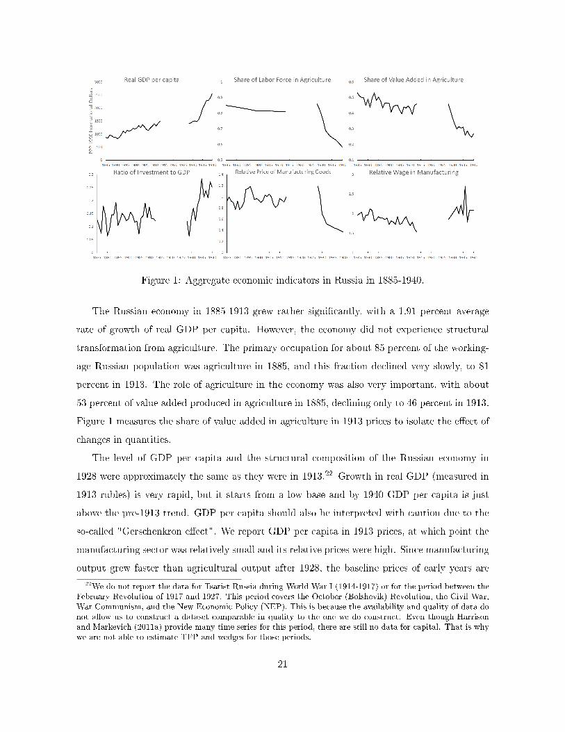
Figure 1: Aggregate economic indicators in Russia in 1885-1940.

The Russian economy in 1885-1913 grew rather signi�cantly, with a 1.91 percent average

rate of growth of real GDP per capita. However, the economy did not experience structural

transformation from agriculture. The primary occupation for about 85 percent of the working-

age Russian population was agriculture in 1885, and this fraction declined very slowly, to 81

percent in 1913. The role of agriculture in the economy was also very important, with about

53 percent of value added produced in agriculture in 1885, declining only to 46 percent in 1913.

Figure 1 measures the share of value added in agriculture in 1913 prices to isolate the e�ect of

changes in quantities.

The level of GDP per capita and the structural composition of the Russian economy in

1928 were approximately the same as they were in 1913.22 Growth in real GDP (measured in

1913 rubles) is very rapid, but it starts from a low base and by 1940 GDP per capita is just

above the pre-1913 trend. GDP per capita should also be interpreted with caution due to the

so-called "Gerschenkron e�ect". We report GDP per capita in 1913 prices, at which point the

manufacturing sector was relatively small and its relative prices were high. Since manufacturing

output grew faster than agricultural output after 1928, the baseline prices of early years are

22We do not report the data for Tsarist Russia during World War I (1914-1917) or for the period between theFebruary Revolution of 1917 and 1927. This period covers the October (Bolshevik) Revolution, the Civil War,War Communism, and the New Economic Policy (NEP). This is because the availability and quality of data donot allow us to construct a dataset comparable in quality to the one we do construct. Even though Harrisonand Markevich (2011a) provide many time series for this period, there are still no data for capital. That is whywe are not able to estimate TFP and wedges for those periods.

21

particularly favorable to show high rates of GDP growth. There is little doubt that structural

transformation was very rapid in 1928-1940. The labor force in manufacturing almost tripled

during this time period and the expansion of this sector was much more rapid.

5 Wedge decomposition

Figure 2 presents the total factor productivities XMt , XA

t and the wedges 1 + τW,t, 1 + τR,t and

1 + τK,t. The dashed lines are the Tsarist trend growth rates for XMt and XA

t and the average

values of quantity wedges in 1885-1913 (with the exclusion of the famine years in the early

1890s) for a comparison with the frictions in the Soviet economy.

Figure 2: Aggregate distortions in Russia in 1885-1940.

Figure 3 shows the decomposition of the wedges 1+τW,t and 1+τR,t into their components.

Since there are no data on the sectoral capital rental rates, the decomposition is done under

the assumption that the mobility component of the inter-sector capital wedge is zero. In our

discussion of the results we mainly focus on the labor wedge decomposition since we can measure

its components more precisely.

22

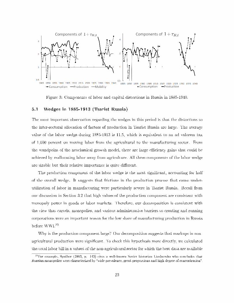
Figure 3: Components of labor and capital distortions in Russia in 1885-1940.

5.1 Wedges in 1885-1913 (Tsarist Russia)

The most important observation regarding the wedges in this period is that the distortions to

the inter-sectoral allocation of factors of production in Tsarist Russia are large. The average

value of the labor wedge during 1885-1913 is 11.5, which is equivalent to an ad valorem tax

of 1,050 percent on moving labor from the agricultural to the manufacturing sector. From

the standpoint of the neoclassical growth model, there are large e�ciency gains that could be

achieved by reallocating labor away from agriculture. All three components of the labor wedge

are sizable but their relative importance is quite di�erent.

The production component of the labor wedge is the most signi�cant, accounting for half

of the overall wedge. It suggests that frictions in the production process that cause under-

utilization of labor in manufacturing were particularly severe in Tsarist Russia. Recall from

our discussion in Section 3.2 that high values of the production component are consistent with

monopoly power in goods or labor markets. Therefore, our decomposition is consistent with

the view that cartels, monopolies, and various administrative barriers to creating and running

corporations were an important reason for the low share of manufacturing production in Russia

before WWI.23

Why is the production component large? Our decomposition suggests that markups in non-

agricultural production were signi�cant. To check this hypothesis more directly, we calculated

the total labor bill in a subset of the non-agricultural sector for which the best data are available

23For example, Spulber (2003, p. 143) cites a well-known Soviet historian Liashcenko who concludes thatRussian monopolies were characterized by �wide prevalence, great proportions and high degree of concentration�.

23

� factories. Gregory (1982) reports that the value added in factories was 3 bln rubles in 1913,

and employment records show that factories employed 2.3 mln people (Gregory, 1972). Factory

surveys during the Tsarist period show that the average annual wage in factories was 257 rubles

in that year (Allen, 2001, Strumilin, 1960), which implies that the total wage bill was less than

20 percent of the total factory value added. Standard estimates of the labor share in production

are in the range of 60-70 percent, which implies a markup of 3-3.5, remarkably close to the

average markup of 3.14 that we obtain through our decomposition.24

The labor mobility component is sizable but it is the smallest out of the three components,

and its relative signi�cance further falls after 1895. Its average value of 1.85 implies that manu-

facturing wages are 85 percent higher than agricultural wages. Higher wages in manufacturing

are a common historical phenomenon, and such factors as costly skill acquisition or higher ur-

ban living expenses can partially account for that.25 The agricultural policies in Tsarist Russia

that discouraged labor mobility (see our discussion of communes in Sections 2 and 3.2) are

the residual of this component, once wages are adjusted for those factors. Therefore, policies

that discourage labor mobility are unlikely to play a signi�cant quantitative role in the low

labor share in manufacturing. Contrary to the views of Lenin, Gerschenkron and many others,

Russian communes do not appear to be among the main barriers to structural transformation.26

The consumption component of the labor wedge is sizable. This is consistent with the

evidence that di�erent regional markets were poorly integrated and that many Russian farmers

were "subsistence-oriented" producing only a small fraction of their income for commercial sale.

As we showed in Section 3.2, costly access to centralized markets maps into a positive price

component in our decomposition.27

24The importance of the production component decreases if a country adopts less labor intensive technologies,that is, chooses technologies for which αM,N is lower. This choice would be optimal for countries which arerelatively abundant in capital and scarce in labor which is contrary to the evidence on relative factor abundancein Russia at the beginning of the 20th century.

25See Caselli and Coleman (2001) for the emphasis on skill composition and its implications for the behaviorof prices and wages in the neoclassical growth model. Allen (2003) discusses the importance of skill acquisitionin the Russian economy. The only wage series we have for manufacturing workers that contains informationabout skills is the time series for construction workers in St Petersburg from Strumilin (1960). The wagesfor an unskilled construction worker (chernorabochij ) in that data set are about 50% higher than the averageagricultural wages in the European provinces of the Russian empire.

26This �nding is consistent with the recent work by economic historians who used the available micro-datato study the causal e�ect of communal land holdings on rural-urban migration. Gregory (1994) argues thatcommunal restrictions on rural-urban migration were not signi�cant. Borodkin, Granville, and Leonard (2008)use time series evidence for the St Petersburg region and Nafziger (2010) analyzes a household-level dataset ofvillages in the Moscow province to reach similar conclusions.

27See also Spulber (2003, p. 101) for various administrative measures that hampered domestic trade. Spulber

24

5.2 Wedges 1928-1940 (Soviet Russia)

The analysis of Figures 2 and 3 reveals two broad patterns during 1928-40. The total factor

productivity performs poorly in both sectors (it is signi�cantly below Tsarist trends for most

of the sample), and all the wedges fall relative to their average Tsarist levels. The drop in

the labor wedge is fully accounted for by the drop in its production component. By 1935,

this component reaches the level predicted by the neoclassical growth model. The other two

components of the labor wedge increase, especially after 1935.

To quantify the contribution of each component of our wedge decomposition to growth

and to changes in the agricultural labor share we perform the following procedure. We �rst

compute the path of the economy holding all wedges �xed at their 1928 levels.28 Even with all

the wedges �xed, GDP still grows at 1.2 percent per year, and the labor share decreases by 0.9

percent. This is due to the fact that the initial capital in 1928 is lower than the steady state,

hence, convergence to the steady state generates some growth and structural transformation

(row 9, Capital Accumulation K0). We then re-compute the path of the economy when all

exogenous variables (including wedges and productivities) are set to values that we observe in

the data. When all those series are set to the values observed in the data, the model matches

the observed quantities and prices in the data exactly. We compare the simulated path with

�xed wedges with the actual historical path by computing the di�erence between the rates of

growth of annual GDP and the di�erence between the changes in the agricultural labor share

from 1928 to 1939. Finally, we compute the contributions of wedges and TFPs by adding

exogenous variables subsequently one by one and computing the relative changes in GDP and

the labor share at each step.

The numbered rows in Table 2 report the marginal contribution of each factor. The exact

numbers slightly depend on the order in which we add wedges and other series, and we report

the average values after taking 1000 random draws of the order in which we add exogenous

(p. 111) gives the statistics on how ine�cient and limited the Russian railroad system was. For example, atthe end of 1913, Russia had only 1/12th of railroad coverage in terms of kilometers of railway per 100 squarekilometers of territory, compared to Great Britain, Ireland and Germany. Spulber (p. 76) concludes that �themajor part of the peasant farms constituted a subsistence sector, and the limited rest, a commercialized sector�.

28The system of feasibility conditions (6), (7) and market clearing conditions (8)-(10) for 1928-1940 consists ofZ unknown variables and Z − 1 equations. An additional assumption is needed to either determine the level ofinvestment I1940 or expected consumption in manufacturing CM1941. We experimented with di�erent assumptionsto pin down the last expression all producing similar results (see the working paper Cheremukhin et al (2013)and especially its computational appendix). The experiments in our baseline speci�cation assume that after1941 the TFPs continue to grow with their trend rates, and the wedges remain at their levels of the late 1930s.

25

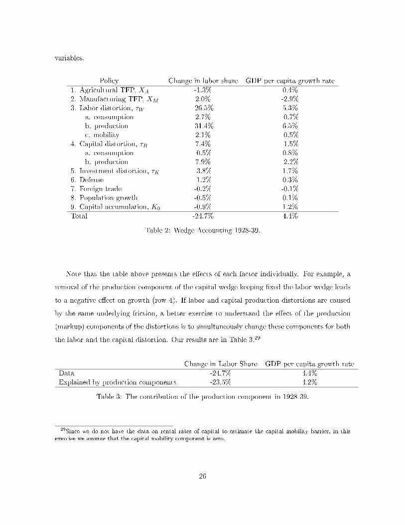
variables.

Policy Change in labor share GDP per capita growth rate

1. Agricultural TFP, XA -1.3% 0.4%2. Manufacturing TFP, XM 2.0% -2.9%3. Labor distortion, τW -26.5% 5.3%

a. consumption 2.7% -0.7%b. production -31.4% 6.5%c. mobility 2.1% -0.5%

4. Capital distortion, τR 7.4% -1.5%a. consumption -0.5% 0.8%b. production 7.9% -2.2%

5. Investment distortion, τK -3.8% 1.7%6. Defense -1.2% 0.3%7. Foreign trade -0.2% -0.1%8. Population growth -0.5% 0.1%9. Capital accumulation, K0 -0.9% 1.2%

Total -24.7% 4.4%

Table 2: Wedge Accounting 1928-39.

Note that the table above presents the e�ects of each factor individually. For example, a

removal of the production component of the capital wedge keeping �xed the labor wedge leads

to a negative e�ect on growth (row 4). If labor and capital production distortions are caused

by the same underlying friction, a better exercise to understand the e�ect of the production

(markup) components of the distortions is to simultaneously change these components for both

the labor and the capital distortion. Our results are in Table 3.29

Change in Labor Share GDP per capita growth rate

Data -24.7% 4.4%Explained by production components -23.5% 4.2%

Table 3: The contribution of the production component in 1928-39.

29Since we do not have the data on rental rates of capital to estimate the capital mobility barrier, in thisexercise we assume that the capital mobility component is zero.

26

Our decomposition shows that the policies that reduced the relative production distortions

between the two sectors led to a reallocation of labor towards manufacturing and to higher

growth rates in per capita GDP in 1928-39. Recall that the high level of the production

component in the Tsarist economy is consistent with monopolists in the manufacturing sector

optimally deciding to reduce their output in order to increase pro�t. In such circumstances

any policy that encourages manufacturing producers to expand output should on the margin

reduce the markup in the manufacturing sector, reduce the production component of the labor

distortion, and reallocate labor from agriculture to manufacturing. Removal of entry barriers

and encouragement of competition are examples of such policies in competitive economies.

In the Soviet economy, the central government incentivized enterprise managers to achieve

ambitious production targets rather than to maximize pro�t, and channeled resources into

industry, which also led to an expansion of industrial output, to reallocation of labor, and to

a reduction in the production component of the inter-sectoral labor wedge. Soviet agricultural

policies may have also contributed to the reduction of the production component. As we

discussed in Section 3.2, the allocation of resources between sectors depends on the relative

markups in the two sectors. An increase in monopsony power of agricultural producers, due to

the policy of collectivization and a ban on private commercial farming, allows them to in�uence

wages paid in the agricultural sector and to increase markups there. Such policies also reduce

the production component of the labor wedge and push labor out of agriculture.

Our �ndings are inconsistent with the predictions of �Big Push� theories that sweeping state

investments should increase productivity in the manufacturing sector and increase the labor

wedge (see Section 3.2). We observe exactly the opposite. The labor wedge signi�cantly de-

creased. TFP fell in both sectors during the main phases of industrialization and collectivization

and remained signi�cantly below Tsarist trends in most years.

The behavior of sectoral TFPs is consistent with a view that the Soviet economy, although

successful in reallocating resources towards manufacturing, failed to provide the right conditions

for e�cient utilization of those resources within each sector. While part of the productivity

drop can be accounted for by other factors, such as the large in�ow of relatively inexperienced,

low-skill workers into manufacturing, the poor performance of agricultural productivity and

output are particularly illustrative. Davies, Harrison and Wheatcroft (1994) trace the drop in

agricultural output to several factors. They argue that the state exaction of grain from peasants

27

on its own created dramatic disruptions to agricultural production by reducing incentives to

work on collectivized land, by disrupting the system of crop rotation, and by a drastic fall in the

number of draught animals. Moreover, the dekulakization campaign led to exile and execution

of the most successful and knowledgeable peasants. All these factors are consistent with an

ine�ciently managed transition process.

The e�ect of the reduction in agricultural output on population is another glaring example

of the ine�ciencies of Soviet policies. Although agricultural production dropped in 1931-33

relative to its 1928 level, in per capita terms it was still above the levels of production in the

late 19th century. Since total agricultural output exceeded subsistence needs, any increase in

mortality could be avoided. Instead, Soviet policies of food collection and distribution led to

the most severe famine in Russian history, resulting in millions of deaths.30,31

Our decomposition in Table 2 also shows that such factors as the increase in military

expenditures in the late 1930s and the reduction in international trade played some role in the

reallocation of labor towards manufacturing, but the e�ect of these factors is relatively small.

Similarly, the contributions of sectoral total factor productivities are relatively small, which

illustrates that the channels of structural change typically emphasized in the literature (see,

e.g. Chapter 20 in Acemoglu, 2008), played a minor role in the structural transition of the

Soviet Union.

5.3 The role of the production component of the distortions

Our analysis suggests that distortions in manufacturing, consistent with monopolistic behavior,

were among the main factors hindering structural change in Tsarist Russia, and that the removal

of such distortions was the main mechanism through which labor re-allocation occurred in the

Soviet economy. This �nding is consistent with a number of recent papers that emphasize the

30Davies, Harrison and Wheatcroft (1994) review di�erent available estimates and conclude (p. 77) that �thetotal number of the excess deaths may have amounted to 8.5 million in 1927-36 ... most of the deaths took placeduring the 1933 famine.�

31Meng, Qian and Yared (2014) provide important evidence on the causes of famine in another centrally-planned economy, China, in 1959-61. They identify poor information �ows within the government as the mainreason for high mortality. Many features of the two famines are very similar. In both cases, although therewas su�cient food production to avoid malnutrition, government policies led to relative scarcity of food in thecountryside compared with the cities, and the most fertile regions experienced some of the most severe famines.The similarity of institutions and outcomes in the two economies suggests that similar mechanisms are likely tohave led to high mortality rates in Soviet Russia in 1931-33.

28

negative e�ect of monopolies on growth.32 This literature typically emphasizes that monopolies

may lower productivity in a given sector. Our �ndings also indicate that monopolies further

lower welfare by creating a barrier to e�cient allocation of resources between sectors.

In this section, we investigate the e�ect of monopoly distortions on Tsarist Russia.33 We

conduct the following experiment. We �x all the wedges, exports, and government expendi-

tures at their 1913 levels and extrapolate the economy forward using trend TFP growth rates

from 1885-1913. We compare this simulation with an alternative extrapolation in which all

production distortions are reduced to zero, while the remaining components are kept at their

1913 levels. This experiment allows us to evaluate welfare losses due to deviations from e�cient

choices of competitive �rms in both sectors.

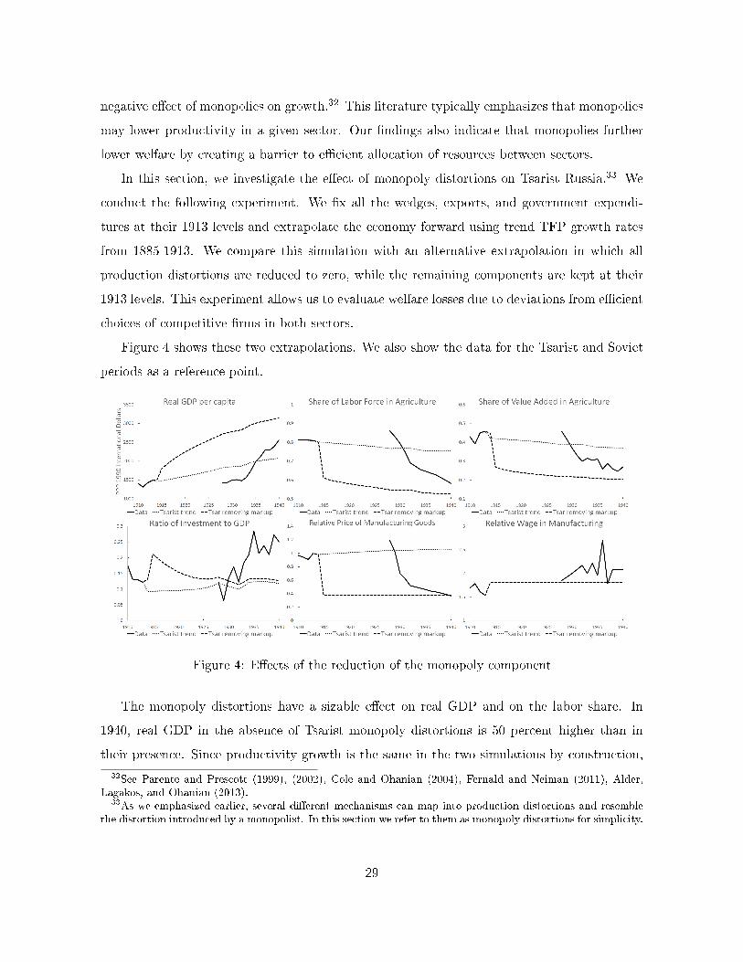
Figure 4 shows these two extrapolations. We also show the data for the Tsarist and Soviet

periods as a reference point.

Figure 4: E�ects of the reduction of the monopoly component

The monopoly distortions have a sizable e�ect on real GDP and on the labor share. In

1940, real GDP in the absence of Tsarist monopoly distortions is 50 percent higher than in

their presence. Since productivity growth is the same in the two simulations by construction,

32See Parente and Prescott (1999), (2002), Cole and Ohanian (2004), Fernald and Neiman (2011), Alder,Lagakos, and Ohanian (2013).

33As we emphasized earlier, several di�erent mechanisms can map into production distortions and resemblethe distortion introduced by a monopolist. In this section we refer to them as monopoly distortions for simplicity.

29

all additional GDP growth is achieved through reallocation of labor and accumulation of cap-

ital. Because the manufacturing sector is more capital intensive, the elimination of monopoly

distortions generates an initial investment boom. It also leads to a reallocation of about 30

percent of the labor force towards manufacturing and a drop in the relatives prices of manu-

facturing goods by about 60 percent. The permanent removal of monopoly distortions leads to

a welfare gain equivalent to a 27.4 percent permanent increase in aggregate consumption.

The predictions of the neoclassical growth model for the behavior of labor allocations and

prices due to the removal of the production component of distortions are notably consistent

with the behavior of those variables in the Soviet data. Recall that in the data the production

component of distortions reduced almost to one by 1935. The observed drop in relative prices

in Soviet Russia and the reallocation of labor are remarkably consistent with the simulated

response of the economy. This is consistent with the fact that the production components in

Table 2 account for most of the growth and most of the labor transformation. The behavior

of prices in the data is also consistent with the view of economic historians that prices played

an important allocative role in the Soviet economy and arose as an outcome of a decentralized

bargaining process between Soviet enterprises and government ministries rather than from being

set in an arbitrary fashion.34

Our analysis also gives an insight on a classical debate in development economics on "push"

versus "pull" theories of development, whether it is the development of modern industry that

attracts ("pulls") workers by a higher wage or it is rapid productivity growth in agriculture that

"pushes" workers out of that sector.35 We �nd that the "pull" forces played a central role in

the growth experience of Russia in 1885-1940. We �nd that distortions in production, such as

barriers to entry and competition, were likely a signi�cant block to a more e�cient allocation of

resources between sectors in Tsarist Russia. Structural transformation in 1928-40 was mainly

34An early comprehensive study of Soviet prices by Harrison (1998) based on the archives of the former Sovietplanning commission and the statistical o�ce argues that �The [planned] prices were quite distinct from theprices currently prevailing in the Soviet economy at any given time, wholesale and retail, regulated and free-market. These currently prevailing prices played important roles, even in a planned economy ...� Gregory andHarrison (2005) based on the recently revealed Stalin's archives argue in favor of rational allocative price settingby Soviet �rms: �Final allocations of products were achieved through contracting between ministries, ministrymain administrations, and enterprises. Decentralized contracting generated a degree of price �exibility, and thistells us much about the motivations, resources, and constraints of the agents involved ... The archives showthat price-setting was one of the most important activities of Soviet �rms ...�. See also our discussion of pricesetting in the Soviet economy in Section 2.

35Lewis (1954) and Harris and Todaro (1970) are the seminal papers on labor pull. Nurkse (1953), Schultz(1953), and Rostow (1960) are seminal works on labor push.

30

achieved through the removal of such blocks. While productivity in Soviet agriculture was at or

below the Tsarist trend, the reduction in markups and the increase in demand for labor seems

to have played a critical role in Russia's structural transformation.36

5.4 Robustness

In this section we discuss the results of alternative parametrizations of our model. We in-

vestigate three sets of parameters: parameters governing the factor shares in production, α,

parameters governing the degree of non-homotheticity, γ, and the elasticity of substitution, σ.

We summarize the implications of these parameters for our decomposition of structural change

and growth in 1928-39 in Table 4. In all simulations, the changes in the production components

of the labor and capital wedges play the largest quantitative role. We comment on the speci�c

details below.

To compute the results presented in each column of Table 4, we changed the values of

some of the parameters and kept the remaining parameters unchanged. In the �rst robustness

exercise, we changed σ from 1 to 0.5; in the second, we changed γ from 29 to 0; in the third,

we set αN,M = αN,A = αK,M = 0.5 and kept the returns to scale in agriculture unchanged by

setting αK,A = 0.31. In each of three cases, we re-computed the paths of the wedges and then

re-produced the wedge accounting exercise from Section 5.2 for the new set of parameters.

First, we want to make several general observations. The assumptions regarding the degree

of non-homotheticity and the factor shares mainly a�ect the levels of wedges but not their

contributions to growth or labor reallocation. The contributions to growth and labor realloca-

tion are primarily driven by changes in the wedges, which, in turn, are determined by changes

in the capital-labor ratios and the prices observed in the data. Assuming lower labor shares,

αN,i, for example, implies a somewhat lower absolute level of the production component in the

Tsarist economy and the Soviet economy, but the relative fall of this component is essentially

unchanged. For this reason, the contribution of the production component with the labor share

set to 0.5 is roughly the same as in our baseline simulation. Although the absolute value of the

component is somewhat reduced, it remains the most signi�cant component of the labor wedge

before 1913.

36We, however, are not claiming that "push" forces are not important. Our model predicts that a largeincrease in agricultural productivity would also lead to structural change; we do not observe such an increasein the Soviet data.

31

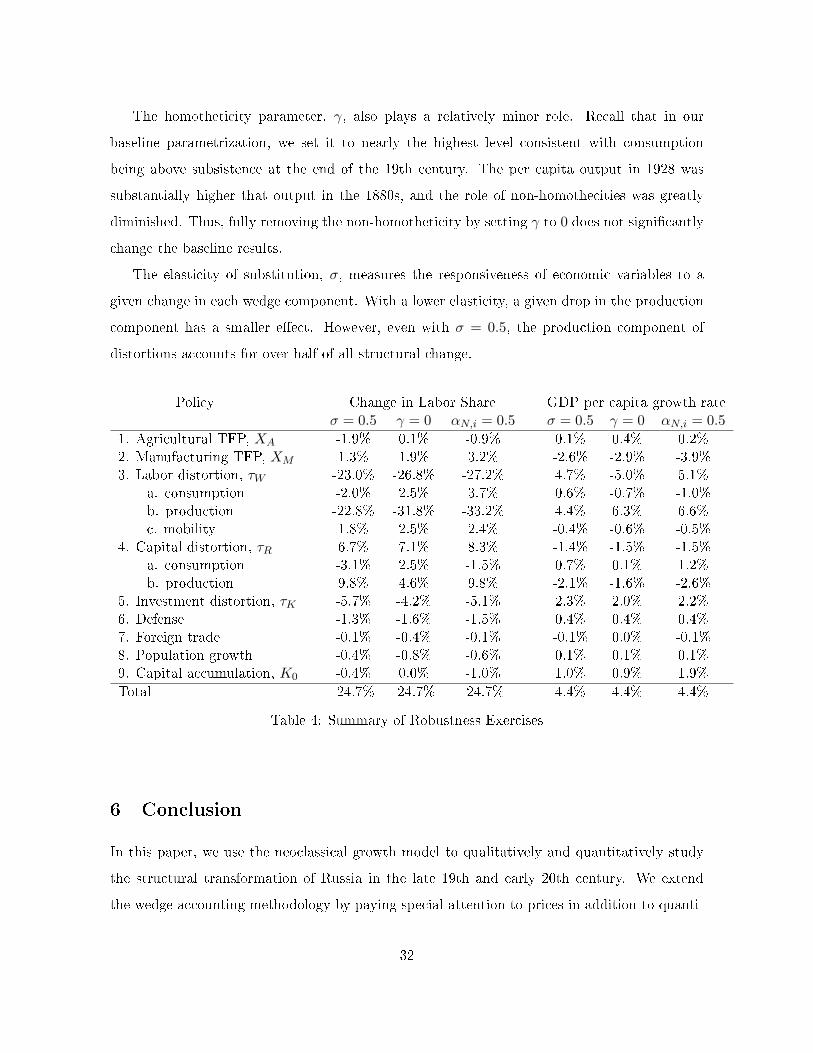
The homotheticity parameter, γ, also plays a relatively minor role. Recall that in our

baseline parametrization, we set it to nearly the highest level consistent with consumption

being above subsistence at the end of the 19th century. The per capita output in 1928 was

substantially higher that output in the 1880s, and the role of non-homothecities was greatly

diminished. Thus, fully removing the non-homotheticity by setting γ to 0 does not signi�cantly

change the baseline results.

The elasticity of substitution, σ, measures the responsiveness of economic variables to a

given change in each wedge component. With a lower elasticity, a given drop in the production

component has a smaller e�ect. However, even with σ = 0.5, the production component of

distortions accounts for over half of all structural change.

Policy Change in Labor Share GDP per capita growth rateσ = 0.5 γ = 0 αN,i = 0.5 σ = 0.5 γ = 0 αN,i = 0.5

1. Agricultural TFP, XA -1.9% 0.1% -0.9% 0.1% 0.4% 0.2%2. Manufacturing TFP, XM 1.3% 1.9% 3.2% -2.6% -2.9% -3.9%3. Labor distortion, τW -23.0% -26.8% -27.2% 4.7% -5.0% 5.1%

a. consumption -2.0% 2.5% 3.7% 0.6% -0.7% -1.0%b. production -22.8% -31.8% -33.2% 4.4% 6.3% 6.6%c. mobility 1.8% 2.5% 2.4% -0.4% -0.6% -0.5%

4. Capital distortion, τR 6.7% 7.1% 8.3% -1.4% -1.5% -1.5%a. consumption -3.1% 2.5% -1.5% 0.7% 0.1% 1.2%b. production 9.8% 4.6% 9.8% -2.1% -1.6% -2.6%

5. Investment distortion, τK -5.7% -4.2% -5.1% 2.3% 2.0% 2.2%6. Defense -1.3% -1.6% -1.5% 0.4% 0.4% 0.4%7. Foreign trade -0.1% -0.4% -0.1% -0.1% 0.0% -0.1%8. Population growth -0.4% -0.8% -0.6% 0.1% 0.1% 0.1%9. Capital accumulation, K0 -0.4% 0.0% -1.0% 1.0% 0.9% 1.9%

Total -24.7% -24.7% -24.7% 4.4% 4.4% 4.4%

Table 4: Summary of Robustness Exercises

6 Conclusion

In this paper, we use the neoclassical growth model to qualitatively and quantitatively study

the structural transformation of Russia in the late 19th and early 20th century. We extend

the wedge accounting methodology by paying special attention to prices in addition to quanti-

32

ties. Decomposing wedges into their price components allows us to di�erentiate among various

mechanisms that map into the same quantity wedge but have sharply di�erent predictions for

prices. We �nd that the high level of the inter-sectoral labor wedge was the main impediment

to structural transformation of Tsarist Russia, and its reduction played by far the most signif-

icant role during Soviet industrialization. In terms of the analysis of the components of the

labor wedge, we �nd that the distortions to the allocation of resources across sectors, consistent

with the evidence on the importance of monopolies in Tsarist Russia, is the key ingredient of

the labor wedge. The reduction in the degree of misallocation of production in Soviet Russia

explains essentially all of the observed structural transformation. Other components of the

labor wedge become more distorted. Thus, our �ndings on the role of the production compo-

nent of the labor wedge cast doubt on the most common explanation of slow transformation

of Tsarist Russia � that archaic institutions of land ownership precluded labor mobility across

sectors. Our �ndings are also inconsistent with the theory of a �Big Push�. Moreover, we �nd

little evidence that the di�erence in TFP growth across sectors is responsible for structural

transformation.

We believe that our analysis of the most important barriers to the development of Tsarist

Russia and the factors behind Soviet industrialization is useful beyond the interests of economic

history. Our methodology of decomposing wedges into price components is applicable more

broadly to a variety of other settings. Our �ndings on the relative importance of components of

the labor wedge gives further support to the idea that frictions and prices play a signi�cant role

in structural transformation (e.g., Caselli and Coleman, 2001). The fact that misallocation of

resources consistent with e�ects of monopoly distortions plays a key role supports and further

develops the �ndings in the contexts of barriers to riches (Parente and Prescott, 2002), the

U.S. Great Depression (Cole and Ohanian, 2004), and the decline of the U.S. rust belt (Alder,

Lagakos, and Ohanian, 2013). Our �ndings on the limited role of labor mobility restrictions

and the absence of evidence for the role of the �Big Push� is of broader interest to the economic

development literature.

We now brie�y note some other issues that we did not discuss in this paper. First, our

working paper version (Cheremukhin et. al., 2013) provides a much more complete description

of the historical accounts, robustness exercises, and other counterfactuals. Second, we on

purpose avoided the discussion of welfare implications of various policies. Stalin's era was one

33

of the most terrible episodes of Russian history with millions perishing in the famine of the

early 1930s. Any welfare calculation must necessarily take a stand on the costs of the lives lost.

Thirdly, in this paper we did not discuss two periods of Russian history that are of interest

to scholars of Russia. The period of the Civil War and War Communism following the fall

of Tsarist Russia is an example of a signi�cant economic disaster. We refer the reader to an

impressive reconstruction of some of the economic statistics during that period by Harrison

and Markevich (2011a,b). The brief period of the New Economic Policy in the 1920s saw a

reintroduction of a limited market economy in Soviet Russia that was cut short by Stalin. We

refer an interested reader to a detailed analysis of the New Economic Policy in the working

paper version (Cheremukhin et. al., 2013).

7 References

Acemoglu, Daron (2008) Introduction to Modern Economic Growth, Princeton University

Press.

Acemoglu, Daron, and Veronica Guerrieri (2008) �Capital Deepening and Nonbal-

anced Economic Growth,� Journal of Political Economy, 116(3), pp. 467-498.

Alder, Simeon, David Lagakos, and Lee Ohanian (2013) �The Decline of the U.S.

Rust Belt: A Macroeconomic Analysis,� mimeo, UCLA.

Allen, Robert C. (1997) �Agricultural Marketing and the Possibilities for Industrializa-

tion in the Soviet Union in the 1930s,� Explorations in Economic History, 34(4), pp. 387-410.

Allen, Robert C. (2003) Farm to Factory: a Reinterpretation of the Soviet Industrial

Revolution, Princeton University Press.

Barsov, Alexander (1969) Balans Stoimostnykh Obmenov Mezhdu Gorodom i Derevnei.

Moscow: Nauka. [in Russian: The balance of the costs exchange between the city and the village]

Bergson, Abram, Roman Bernaut, and Lynn Turgeon (1955) �Basic Industrial

Prices in the USSR, 1928�1950: Twenty-Five Branch Series and Their Aggregation,� Santa

Monica: The Rand Corporation. Research Memorandum RM-1522.

Borodkin, Leonid, Brigitte Granville, and Carol Leonard (2008) �The Rural/urban

Wage Gap in the Industrialisation of Russia, 1884�1910,� European Review of Economic His-

tory, 12, pp. 67�95.

34

Buera, Francisco and Joe Kaboski (2009) �Can Traditional Theories of Structural

Change Fit the Data?� Journal of the European Economic Association, 7(2-3), pp. 469-477.

Buera, Francisco and Joe Kaboski (2012a) �Scale and the Origins of Structural

Change,� Journal of Economic Theory, 147(2), pp. 684-712.

Buera, Francisco and Joe Kaboski (2012b) �The Rise of the Service Economy,� Amer-

ican Economic Review, 102(6), pp. 2540-69.

Caselli, Francesco (2005) �Accounting for Cross-Country Income Di�erences,� Handbook

of Economic Growth (Aghion and Durlauf, eds.), North-Holland.

Caselli, Francesco, and Wilbur John II Coleman (2001) �The U.S. Structural

Transformation and Regional Convergence: A Reinterpretation,� Journal of Political Econ-

omy, 109(3), pp. 584-616.

Chari, V. V., Patrick Kehoe, and Ellen McGrattan (2007) �Business Cycle Ac-

counting,� Econometrica, 75(3), pp. 781-836.

Cheremukhin, Anton, Mikhail Golosov, Sergei Guriev, and Aleh Tsyvinski

(2013) �Was Stalin Necessary for Russia's Economic Development?� NBER Working Paper

19425.

Chernina, Eugenia, Paul Castaneda Dower, and Andrei Markevich (2014) �Prop-

erty Rights and Internal Migration: The Case of the Stolypin Agrarian Reform in the Russian

Empire.� Journal of Development Economics, forthcoming.

Cole, Harold, and Lee Ohanian (2002) �The U.S. and U.K. Great Depressions Through

the Lens of Neoclassical Growth Theory,� American Economic Review, 92(2), pp. 28-32.

Cole, Harold, and Lee Ohanian (2004) �New Deal Policies and the Persistence of the

Great Depression: A General Equilibrium Analysis,� Journal of Political Economy, 112(4), pp.

779-816.

Crisp, Olga (1978) �Labor and Industrialization in Russia,� Cambridge Economic History

of Europe, Vol. 7, part 2. Cambridge University Press.

Davies, Robert (1990) From Tsarism to the New Economic Policy. Macmillan Academic

and Professional Ltd.

Davies, R.W., Mark Harrison and S.G. Wheatcroft (1994) The Economic Trans-

formation of the Soviet Union, 1913-1945 ; New York : Cambridge University Press.

Davies, R.W., and S.G. Wheatcroft (2004) The Years of Hunger: Soviet Agriculture,

35

1931-1933, Palgrave Macmillan.

Fernald, John, and Brent Neiman (2011) �Growth Accounting with Misallocation:

Or, Doing Less with More in Singapore,� American Economic Journal: Macroeconomics, 3(2),

pp. 29-74.

Gerschenkron, Alexander (1965) �Agrarian Policies and Industrialization, Russia 1861�

1917,� In: Habakkuk, H.J., Postan, M. (Eds.), The Cambridge Economic History of Europe.

Volume VI: The Industrial Revolutions and After: Incomes, Population and Technological

Changes (II). Cambridge University Press, Cambridge, England, pp. 706-800.

Gollin, Douglas, David Lagakos, and Michael E. Waugh (2014) �The Agricultural

Productivity Gap,� Quarterly Journal of Economics, 129 (2): 939-993.

Gollin, Douglas, Stephen Parente, and Richard Rogerson (2002) �The Role of

Agriculture in Development," American Economic Review, 92(2), pp. 160-164.

Gregory, Paul (1972) �Economic Growth and Structural Change in Tsarist Russia: A

Case of Modern Economic Growth?� Soviet Studies, 23(3), pp. 418-434.

Gregory, Paul (1982) Russian National Income, 1885-1913, Cambridge University Press.

Gregory, Paul (1994) Before Command: The Russian Economy From Emancipation to

Stalin, Princeton: Princeton University Press.

Gregory, Paul, and Mark Harrison (2005) �Allocation under Dictatorship: Research

in Stalin's Archives,� Journal of Economic Literature, 43(3), pp. 721-761.

Gregory, Paul, and Robert Stuart (1986) Soviet Economic Structure and Performance.

New York: Harper & Row.

Harris, John R., and Michael P. Todaro (1970) "Migration, Unemployment and De-

velopment: A Two-Sector Analysis,� American Economic Review, 60(1), pp.126-42.

Harrison, Mark (1998) �Prices, Planners, and Producers: An Agency Problem in Soviet

Industry, 1928-1950,� Journal of Economic History 58(4), pp. 1032-1062.

Harrison, Mark and Andrei Markevich (2011a) �Great War, Civil War, and Recovery:

Russia's National Income, 1913 to 1928,� Journal of Economic History, 71(3), pp. 672-703.

Harrison, Mark and Andrei Markevich (2011b) �Russia's National Income: Ap-

pendix� Online appendix.

Hayashi, Fumio, and Edward Prescott (2008) �The Depressing E�ect of Agricultural

Institutions on the Prewar Japanese Economy,� Journal of Political Economy, 116(4), pp. 573-

36

632.

Herrendorf, Berthold, Richard Rogerson, and Akos Valentinyi (2013). �Two Per-

spectives on Preferences and Structural Transformation,� American Economic Review, 103(7),

pp. 2752-89.

Jacks, David S. (2005). �Intra- and International Commodity Market Integration in the

Atlantic Economy, 1800-1913,� Explorations in Economic History, 42(3), pp. 381-413.

Kongsamut, Piyabha, Sergio Rebelo, and Danyang Xie (2001) �Beyond Balanced

Growth,� Review of Economic Studies, 68(4), pp. 869-82.

Lagakos, David, and Michael E. Waugh (2013) "Selection, Agriculture, and Cross-

Country Productivity Di�erences." American Economic Review, 103(2), pp. 948-80.

Lenin, Vladimir (1972) Lenin. Collected works. Vol 2. Progress Publishers, Moscow.

Lewis, W. Arthur (1954) �Economic Development with Unlimited Supplies of Labor,�

Manchester School 22, pp. 139-192.

Malafeev, Alexei (1964) Istoriia Tsenoobrazonaniia v SSSR, 1917-1963. Moskva: Mysl'.

[In Russian: The history of price-setting in the Soviet Union]

Mau, Vladimir, and Tatiana Drobyshevskaya (2013) �Modernization and the Russian

Economy: Three Hundred Years of Catching Up,� in Michael Alexeev and Shlomo Weber, eds.,

The Oxford Handbook of the Russian Economy, Oxford University Press, pp. 29-51.

Meng, Xing, Nancy Qian, and Pierre Yared (2014) �The Institutional Causes of

Famine in China, 1959-61,� mimeo, Yale University.

Moorsteen, Richard H., and Raymond P. Powell (1966) The Soviet Capital Stock,

1928-1962, Homewood, Ill., R. D. Irwin.

Mulligan, Casey (2002) �A Century of Labor�Leisure Distortions,� Working Paper 8774,

National Bureau of Economic Research.

Murphy, Kevin M., Andrei Shleifer and Robert W. Vishny (1989) �Industrializa-

tion and the Big Push.� Journal of Political Economy, 97(5), pp. 1003-1026.

Nafziger, Steven (2010) �Peasant Communes and Factor Markets in late Nineteenth-

century Russia,� Explorations in Economic History, 47(4), pp. 381�402.

Ngai, L. Rachel, and Christopher Pissarides (2007) �Structural Change in a Multi-

sector Model of Growth,� American Economic Review, 97(1), pp. 429-443.

Nurkse, Ragnar (1953) Problems of Capital Formation in Underdeveloped Countries.

37

Oxford: Oxford University Press.

Owen, Thomas (1991) The Corporation under Russian Law, 1800-1917, Cambridge Uni-

versity Press.

Parente, Stephen, and Edward Prescott (1999) �Monopoly Rights: A Barrier to

Riches,� American Economic Review, 89(5), pp. 1216-1233.

Parente, Stephen, and Edward Prescott (2002): Barriers to Riches, MIT Press.

Pipes, Richard (1997) Russia under the Old Regime. Penguin Books.

Restuccia, Diego, Dennis Tao Yang, and Xiaodong Zhu (2008) �Agriculture and

Aggregate Productivity: A Quantitative Cross-country Analysis,� Journal of Monetary Eco-

nomics, 55(2), pp. 234-250.

Rosenstein-Rodan, Paul (1943) �Problems of Industrialization of Eastern and South-

eastern Europe,� Economic Journal, 53 (210/211), pp. 202-11.

Rostow, Walt Whitman (1960) The Stages of Economic Growth, London: Cambridge

University Press.

Schultz, Theodore W. (1953) The Economic Organization of Agriculture. New York:

McGraw-Hill.

Spulber, Nicolas (2003) Russia's Economic Transitions: From Late Tsarism to the New

Millennium, Cambridge University Press.

Strumilin, Stanislav (1960) Ocherki Ekonomicheskoi Istrorii Rossii. Moscow: izda-

tel'stvo sotsial'no-ekonomicheskoi literatury. [In Russian: Essays in Russian economic history.]

Strumilin, Stanislav (1982) Problemy Ekonomiki Truda. Moscow: Nauka. [In Russian:

The problems of labor economics]

Stokey, Nancy (2001). �A Quantitative Model of the British Industrial Revolution, 1780-

1850,� Carnegie-Rochester Conference Series on Public Policy, 55, pp. 55-109.

38

8 Appendix A: Construction of data

8.1 Capital stock

8.1.1 Russia 1885-1913

For Russia in 1885-1913 all data are from Gregory (1982) using 1913 prices. Capital in agri-

culture is a sum of value of livestock (Table H.1), accumulated agricultural equipment (Table

I.1) and net �xed capital stock in agriculture (Table J.1). Agricultural structures include ru-

ral residential structures, and Gregory does not provide a separate estimate of those. Gregory

provides estimates of livestock, and net capital stock but gives investment in agricultural equip-

ment. We derive the stock of agricultural equipment with the perpetual inventory method by

assuming a 5 percent depreciation. Capital stock in non-agriculture is de�ned as the value

of accumulated industrial equipment (Table I.1), net stock of industrial structures (table J.1),

industry inventories (table K.1), and railroads (Table L.1). The values for the stock of struc-

tures, inventory, railroads, and urban housing are taken directly from Gregory while the stock

of accumulated industrial equipment is obtained by perpetual inventory method assuming a 5

percent depreciation.

This de�nition of capital stock includes rural residential housing into agricultural capital

stock but does not include urban residential housing in any measure of capital stock. The

reason for this is as follows. Ideally, we would like to exclude housing stock from all mea-

sures of capital. Gregory does not provide a breakdown of rural capital between residential

and nonresidential. We do not include urban residential housing into non-agricultural capital

stock since the estimates of urban capital stock di�er dramatically for pre-1913 and post-1928

Russia which we view as unrealistic. Total capital stock is de�ned as a sum of capital stock

in agriculture and non-agriculture. We computed investments in each sector from the series of

capital stocks assuming a 5 percent depreciation.

8.1.2 Russia 1928-1940

For Russia in 1928-1940 we use data from Moorsteen and Powell (1966). All data are in 1937

prices. We use the data on the composition of gross residential �xed capital stock (Table 3-3)

to �nd the fraction of urban residential capital stock in gross residential �xed capital stock.

We assumed that the same ratio holds for net residential capital stock (Table T-15) to �nd

39

the value of net urban residential capital stock. We de�ne non-agricultural capital stock as net

nonresidential, nonagricultural capital stock (table T-25). This de�nition includes industrial

�xed structures, equipment and inventories. We de�ne agricultural capital stock as net �xed

capital stock minus net nonresidential nonagricultural capital stock and minus the value of

urban residential housing. Total capital stock is de�ned as a sum of capital stock in agriculture

and non-agriculture.

8.2 Exports and international prices

The data for the total volume of exports and imports for Tsarist Russia are from Gregory

(1982), Table M-1. We use the data from Davies (1990), Table 56, to �nd the composition

of exports and imports for 1913. We assume that the same composition holds for 1885-1913

and compute net exports of agricultural goods and net imports of non-agriculture goods. The

data for the volume of exports and imports for the USSR from 1928 to 1938 are from Davies,

Harrison and Wheatcroft (1994). They provide an index of exports and imports relative to

1913, and we use the numbers for 1913 trade from Gregory (1982) to obtain the volume of

trade in 1913 prices. We impute the values for 1939 and 1940 by assuming that they remain at

the 1938 level. We use the data from Davies (1990), Table 58, to �nd composition of exports and

imports for 1927/1928. We assume that the same composition holds for 1928-1940 and compute

net exports of agricultural goods and net imports of non-agricultural goods. We use data on

Soviet terms of trade from Davies, Harrison and Wheatcroft (1994), table 50. We found no

comparable numbers for the Tsarist period. As a proxy for the international prices of Russian

exports we take wheat prices in the state of New York. The dollar prices for wheat are from

Jacks (2005). The nominal prices de�ated by the US CPI are from the NBER Macrohistory

Database.

8.3 Output, consumption and investment by sector

8.3.1 Russia 1885-1913

We computed investments in each sector from the series of capital stocks assuming a 5 percent

depreciation. We computed GNP from NNP series in Gregory (1982), Table 3.1, by adding

a 5 percent depreciation to the total capital stock. We did not �nd reliable data for value

added in manufacturing and agriculture for all years. Gregory (1982) in Table 3.6 reports that

40

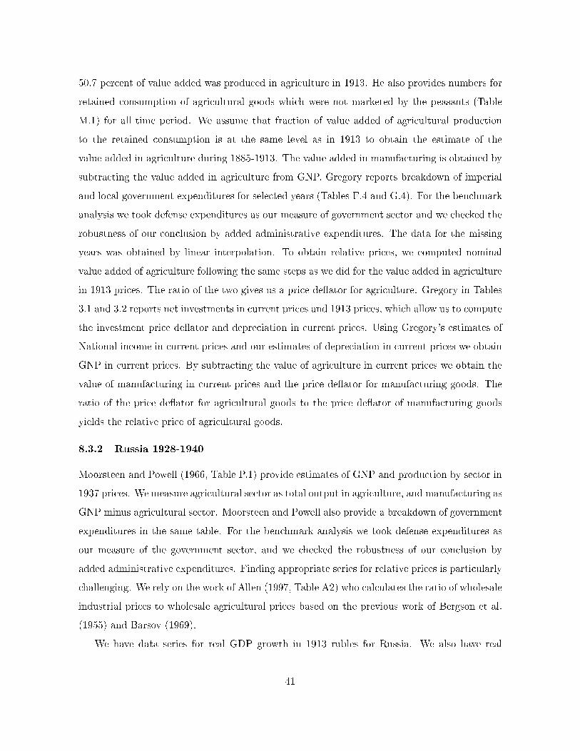
50.7 percent of value added was produced in agriculture in 1913. He also provides numbers for

retained consumption of agricultural goods which were not marketed by the peasants (Table

M.1) for all time period. We assume that fraction of value added of agricultural production

to the retained consumption is at the same level as in 1913 to obtain the estimate of the

value added in agriculture during 1885-1913. The value added in manufacturing is obtained by

subtracting the value added in agriculture from GNP. Gregory reports breakdown of imperial

and local government expenditures for selected years (Tables F.4 and G.4). For the benchmark

analysis we took defense expenditures as our measure of government sector and we checked the

robustness of our conclusion by added administrative expenditures. The data for the missing

years was obtained by linear interpolation. To obtain relative prices, we computed nominal

value added of agriculture following the same steps as we did for the value added in agriculture

in 1913 prices. The ratio of the two gives us a price de�ator for agriculture. Gregory in Tables

3.1 and 3.2 reports net investments in current prices and 1913 prices, which allow us to compute

the investment price de�ator and depreciation in current prices. Using Gregory's estimates of

National income in current prices and our estimates of depreciation in current prices we obtain

GNP in current prices. By subtracting the value of agriculture in current prices we obtain the

value of manufacturing in current prices and the price de�ator for manufacturing goods. The

ratio of the price de�ator for agricultural goods to the price de�ator of manufacturing goods

yields the relative price of agricultural goods.

8.3.2 Russia 1928-1940

Moorsteen and Powell (1966, Table P.1) provide estimates of GNP and production by sector in

1937 prices. We measure agricultural sector as total output in agriculture, and manufacturing as

GNP minus agricultural sector. Moorsteen and Powell also provide a breakdown of government

expenditures in the same table. For the benchmark analysis we took defense expenditures as

our measure of the government sector, and we checked the robustness of our conclusion by

added administrative expenditures. Finding appropriate series for relative prices is particularly

challenging. We rely on the work of Allen (1997, Table A2) who calculates the ratio of wholesale

industrial prices to wholesale agricultural prices based on the previous work of Bergson et al.

(1955) and Barsov (1969).

We have data series for real GDP growth in 1913 rubles for Russia. We also have real

41

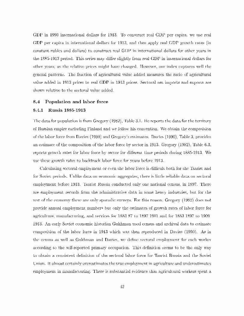
GDP in 1990 international dollars for 1913. To construct real GDP per capita, we use real

GDP per capita in international dollars for 1913, and then apply real GDP growth rates (in

constant rubles and dollars) to construct real GDP in international dollars for other years in

the 1885-1913 period. This series may di�er slightly from real GDP in international dollars for

other years, as the relative prices might have changed. However, our index captures well the

general patterns. The fraction of agricultural value added measures the ratio of agricultural

value added in 1913 prices to real GDP in 1913 prices. Sectoral net imports and exports are

shown relative to the sectoral value added.

8.4 Population and labor force

8.4.1 Russia 1885-1913

The data for population is from Gregory (1982), Table 3.1. He reports the data for the territory

of Russian empire excluding Finland and we follow his convention. We obtain the composition

of the labor force from Davies (1990) and Gregory's estimates. Davies (1990), Table 3, provides

an estimate of the composition of the labor force by sector in 1913. Gregory (1982), Table 6.3,

reports growth rates for labor force by sector for di�erent time periods during 1885-1913. We

use these growth rates to backtrack labor force for years before 1913.

Calculating sectoral employment or even the labor force is di�cult both for the Tsarist and

for Soviet periods. Unlike data on economic aggregates, there is little reliable data on sectoral

employment before 1913. Tsarist Russia conducted only one national census, in 1897. There

are employment records from the administrative data in some heavy industries, but for the

rest of the economy there are only sporadic surveys. For this reason, Gregory (1982) does not

provide annual employment numbers but only the estimates of growth rates of labor force for

agriculture, manufacturing, and services for 1883-87 to 1897-1901 and for 1883-1897 to 1909-

1913. An early Soviet economic historian Gukhman used census and archival data to estimate

composition of the labor force in 1913 which was then reproduced in Davies (1990). As in

the census as well as Gukhman and Davies, we de�ne sectoral employment for each worker

according to the self-reported primary occupation. This de�nition seems to be the only way

to obtain a consistent de�nition of the sectoral labor force for Tsarist Russia and the Soviet

Union. It almost certainly overestimates the true employment in agriculture and underestimates

employment in manufacturing. There is substantial evidence that agricultural workers spent a

42

part of their time in non-agricultural activities, such as seasonal manufacturing work in the city

and self-employment (promysly). We also need to take a stand on how to treat employment

of women. The available employment records before 1913 are from select heavy industries

that predominantly employed men. As the non-agricultural sector expanded dramatically after

1928, so did the fraction of women in non-agricultural employment. Based on this evidence one

may be tempted to conclude that female labor force participation signi�cantly increased. At

the same time, there is evidence that before 1913 female labor force participation in agriculture

was very high, as women had to replace men who were employed as migrant workers in urban

industries. For example, Crisp (1978) in her study of pre-WWI Russian labor markets points

out that although in factory industries there were only 800,000 women compared with several

million men, in peasant farms �the proportion of women undoubtedly exceeded that of male,

especially if all-year-around averages are taken into account�. Since there are no reliable �gures

regarding female labor force participation, we do not treat women and men di�erently and

assume that all of the working age population is a part of the labor force.

Our data on wages for 1885-1913 come from Allen (2003) and Strumilin (1982). The agricul-

tural wages come from the data on male daily wage (Strumilin, 1982, Table 2B, p. 253) which

we then multiply by 205 days per year to obtain the annual wage; according to Table 21, p.

268, agricultural workers worked for 104.2 days in the summer and 100.8 in the winter season.

The non-agricultural wages for 1900-1913 are provided in Strumilin (1982, p. 293). Then we

use we use the data on wages of day laborers and factory workers (Allen, 2003, Figure 2.2)

to calculate the changes in wages in 1885-1900; taking the 1900 level from Strumilin (1982, p.

293) we then calculated the wages in 1885-1899. The data on wages for unskilled construction

workers in St Petersburg is from Strumilin (1960, Table 13, p. 113).

8.4.2 Russia 1928-1940

It is di�cult to obtain reliable data for the composition of the labor force. There have been

three censuses in Russia, in 1926, 1937 and 1939 but the results of the 1937 are mostly un-

published and many historians question reliability of 1939 census. There are o�cial numbers

for employment in various non-agricultural sectors of the economy for select years (Davies,

Harrison and Wheatcroft, 1994, Table 12). Comparing to the Census data, they do not cover

all of the non-agricultural labor force but give a reasonably good approximation of the growth

43

rate of the non-agricultural labor force over the entire time period. According to the census

data, the non-agricultural labor force increased by a factor 3.37 between 1926 and 1939, while

o�cial survey numbers show an increase of 3.19 between 1928 and 1940. We use a procedure

that follows our estimate of Tsarist labor force as closely as possible.

We use population numbers from Davies, Harrison and Wheatcroft (1994), Table 1. From

1926 census (Davies, Harrison and Wheatcroft, 1994, Table 11) we obtain the composition of

the labor force by sector. We assume that each sector covered by the survey data grows at the

same rate as implied by the surveys. This gives us an estimate of non-agricultural labor force

for each year. The implied increase in the labor force is 3.36, which closely matches the implied

growth of non-agricultural labor force from 1939 census. To �nd agricultural labor force we

assume that labor force participation in all years is the same as in 1926 and �nd agricultural

labor force as residual.

This procedure implicitly assumes that the fraction of the labor force to population did not

change between 1926 and 1939. This assumption approximately holds in the data. The ratio

of the labor force to population is 49 percent in 1926 and 50 percent in 1939.

Our data on farm and non-farm wages (consumption) in 1928, 1932-39 come from Allen

(2003, Table 7.5). We use linear interpolation of the ratio of agricultural to non-agricultural

wages for the missing years 1929-31. For the year 1940 we take the ratio of agricultural to

non-agricultural wages from 1939.

8.5 Adjustment for border changes, conversion prices

Using the procedure above we obtained two data sets, one for Russia in 1885-1913 in 1913

borders (excluding Finland) and 1913 prices and the other one for the USSR in 1928-1940 in

pre-1940 borders and 1937 prices. In this section we discuss the conversion of all prices and

quantities to have comparable units. The territory of Russian empire excluding Finland is

21,474 sq km, while the territory of the USSR in pre-1940 borders is 21,242 sq km (Harrison

and Markevich, 2011a, Table 2). Thus the areas of the two territories are quite similar, and

therefore we assume that land endowments are the same in the two periods and do not make

any border adjustments.37

37While land endowment remained the same, Russian empire lost richer territories (Finland, Poland, WesternBelarus and Ukraine, Caucasus) and gained poorer territories in Central Asia. Tsarist NNP in 1913 measuredin the USSR interwar borders would decrease from 22 mln rbl to 16.5 mln rbl (Harrison and Markevich, 2011a,

44

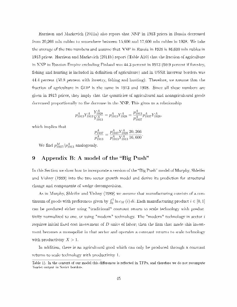
Harrison and Markevich (2011a) also report that NNP in 1913 prices in Russia decreased

from 20,266 mln rubles to somewhere between 15,600 and 17,600 mln rubles in 1928. We take

the average of the two numbers and assume that NNP in Russia in 1928 is 16,600 mln rubles in

1913 prices. Harrison and Markevich (2011b) report (Table A10) that the fraction of agriculture

in NNP in Russian Empire excluding Finland was 44.3 percent in 1913 (50.9 percent if forestry,

�shing and hunting is included in de�nition of agriculture) and in USSR interwar borders was

44.4 percent (50.8 percent with forestry, �shing and hunting). Therefore, we assume that the

fraction of agriculture in GDP is the same in 1913 and 1928. Since all these numbers are

given in 1913 prices, they imply that the quantities of agricultural and nonagricultural goods

decreased proportionally to the decrease in the NNP. This gives us a relationship

pA1913YA

1913

Y A1928

Y A1913

= pA1913YA

1928 =pA1913

pA1937

pA1937YA

1928,

which implies thatpA1937

pA1913

=pA1937Y

A1928

pA1913YA

1913

20, 266

16, 600.

We �nd pM1937/pA1913 analogously.

9 Appendix B: A model of the �Big Push�

In this Section we show how to incorporate a version of the �Big Push� model of Murphy, Shleifer

and Vishny (1989) into the two sector growth model and derive its prediction for structural

change and components of wedge decomposition.

As in Murphy, Shleifer and Vishny (1989) we assume that manufacturing consists of a con-

tinuum of goods with preferences given by´ 1

0 ln cM (i) di. Each manufacturing product i ∈ [0, 1]

can be produced either using "traditional" constant return to scale technology with produc-

tivity normalized to one, or using "modern" technology. The "modern" technology in sector i

requires initial �xed cost investment of D units of labor; then the �rm that made this invest-

ment becomes a monopolist in that sector and operates a constant returns to scale technology

with productivity X > 1.

In addition, there is an agricultural good which can only be produced through a constant

returns to scale technology with productivity 1.

Table 1). In the context of our model this di�erences is re�ected in TFPs, and therefore we do not recomputeTsarist output in Soviet borders.

45

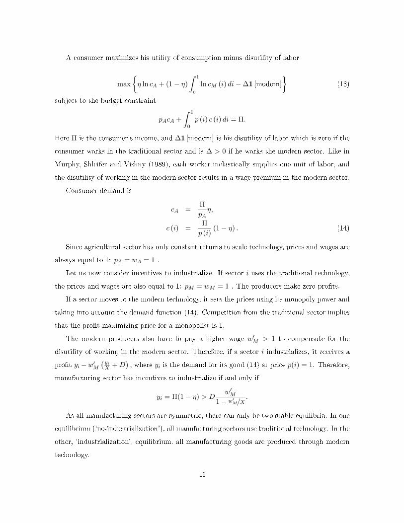
A consumer maximizes his utility of consumption minus disutility of labor

max

{η ln cA + (1− η)

ˆ 1

0

ln cM (i) di−∆1 [modern]

}(13)

subject to the budget constraint

pAcA +

ˆ 1

0p (i) c (i) di = Π.

Here Π is the consumer's income, and ∆1 [modern] is his disutility of labor which is zero if the

consumer works in the traditional sector and is ∆ > 0 if he works the modern sector. Like in

Murphy, Shleifer and Vishny (1989), each worker inelastically supplies one unit of labor, and

the disutility of working in the modern sector results in a wage premium in the modern sector.

Consumer demand is

cA =Π

pAη,

c (i) =Π

p (i)(1− η) . (14)

Since agricultural sector has only constant returns to scale technology, prices and wages are

always equal to 1: pA = wA = 1 .

Let us now consider incentives to industrialize. If sector i uses the traditional technology,

the prices and wages are also equal to 1: pM = wM = 1 . The producers make zero pro�ts.

If a sector moves to the modern technology, it sets the prices using its monopoly power and

taking into account the demand function (14). Competition from the traditional sector implies

that the pro�t maximizing price for a monopolist is 1.

The modern producers also have to pay a higher wage w′M > 1 to compensate for the

disutility of working in the modern sector. Therefore, if a sector i industrializes, it receives a

pro�t yi−w′M( yiX +D

), where yi is the demand for its good (14) at price p(i) = 1. Therefore,

manufacturing sector has incentives to industrialize if and only if

yi = Π(1− η) > Dw′M

1− w′M/X.

As all manufacturing sectors are symmetric, there can only be two stable equilibria. In one

equilibrium ('no-industrialization'), all manufacturing sectors use traditional technology. In the

other, 'industrialization', equilibrium, all manufacturing goods are produced through modern

technology.

46

When manufacturing does not industrialize, the equilibrium is analogous to our baseline

frictionless economy. In particular, from optimality conditions

1− ηη

cAcM

pApM

= 1,

the fact that pM = pA = 1 , and cj = Nj , we get

1− ηη

NA

NM= 1,

NA +NM = 1.

Therefore

NA = η; NM = 1− η.

The consumer's income is Π = 1. This equilibrium exists if and only if

1− η < Dw′M

1− w′M/X, (15)

Let us now consider the equilibrium where all manufacturing �rms industrialize. We still

have p′M = p′A = 1, but now

1− ηη

N ′AXN ′M

= 1,

N ′A +N ′M +D = 1.

This immediately implies

N ′A =(1−D) ηX

1− η + ηX, N ′M =

(1−D) (1− η)

1− η + ηX.

The consumer's income is

Π′ = pAcA + pMcM = XN ′M +N ′A =(1−D)X

1− η + ηX.

The wages in manufacturing are pinned down by ln (Π′ − (w′M − 1)) = ln (Π′)−∆ which implies

w′M = 1 +(1−D)X

1− η + ηX

(1− e−∆

).

The industrialization equilibrium exists whenever

Π′(1− η) > Dw′M

1− w′M/X. (16)

47

If the �xed cost of industrialization D is su�ciently low and the productivity in the modern

sector X is su�ciently high then Π′ = (1−D)X1−η+ηX > Π = 1 so that for some range of ∆ both (15)

and (16) hold. In this case there is a multiplicity of equilibria (and therefore a rationale for the

�Big Push�).

Let us now compare the two equilibria. In the industrialization equilibrium, TFP in man-

ufacturing is higher:XN ′MN ′M + F

> w′M > 1.

Mark up in manufacturing is also higher:

X

w′M>N ′M + F

N ′M> 1.

The ratio of wages in manufacturing and agriculture is also higher:

w′Mw′A

= w′M > 1 =wMwA

.

The ratio prices and the ratio of marginal utilities are the same in both equilibria. The nor-

malized labor wedge isX > 1 in the industrialization equilibrium and 1 in the no-industrialization

equilibrium.

Whenever both equilibria exist, the labor force in agriculture is higher in the industrializa-

tion equilibrium:

N ′A =(1−D) ηX

1− η + ηX> NA = η.

The intuition for this result is straightforward. The industrialization equilibrium exists if and

only if industrialization results in higher aggregate income Π′ > Π. This in turn implies that

industrialization results in a higher demand for agricultural products. As the technology in

agriculture does not change, increase in agricultural production requires an increase in agri-

cultural employment. The labor moves to agriculture from manufacturing (where higher TFP

allows to produce more output with less labor).

48