The Industrialization and Economic Development of Russiathrough the Lens of a Neoclassical Growth Model∗

Anton Cheremukhin, Mikhail Golosov, Sergei Guriev, Aleh Tsyvinski

November 2015

Abstract

This paper studies the structural transformation of Russia in 1885-1940 from an agrarian toan industrial economy through the lens of a two-sector neoclassical growth model. We constructa dataset that covers Tsarist Russia during 1885-1913 and Soviet Union during 1928-1940. Wedevelop a methodology that allows us to identify the types of frictions and economic mech-anisms that had the largest quantitative impact on Russian economic development. We findthat entry barriers and monopoly power in the non-agricultural sector were the most impor-tant reason for Tsarist Russia’s failure to industrialize before World War I. Soviet industrialtransformation after 1928 was achieved primarily by reducing such frictions, albeit coincidingwith a significantly lower performance of productivity in both agricultural and non-agriculturalsectors. We find no evidence that Tsarist agricultural institutions were a significant barrier tolabor reallocation to manufacturing, or that “Big Push” mechanisms were a major driver ofSoviet growth.

∗Cheremukhin: Federal Reserve Bank of Dallas; Golosov: Princeton; Guriev: Sciences Po, Paris, and CEPR;Tsyvinski: Yale. The authors thank Mark Aguiar, Paco Buera, V.V. Chari, Hal Cole, Raquel Fernandez, JosephKaboski, Andrei Markevich, Joel Mokyr, Lee Ohanian, Richard Rogerson, and four anonymous referees for usefulcomments. We also thank participants at Berkeley, Brown, Duke, EIEF, Federal Reserve Bank of Philadelphia,Harvard, HEC, NBER EFJK Growth, Development Economics, and Income Distribution and Macroeconomics,New Economic School, Northwestern, Ohio State, Paris School of Economics, Princeton, Sciences Po, Universityof Zurich. We are particularly indebted to Bob Allen for sharing his data. Financial support from the NSFis gratefully acknowledged. Golosov and Tsyvinski also thank Einaudi Institute of Economics and Finance forhospitality. Any opinions, findings, and conclusions or recommendations expressed in this publication are thoseof the authors and do not necessarily reflect the views of their colleagues, the Federal Reserve Bank of Dallasor the Federal Reserve System.

1 Introduction

The focus of our paper is on the impediments to and mechanisms of structural transformation

from agriculture to industry. Traditionally, the mechanisms of structural transformation are

based on non-homothetic preferences and uneven technical progress across sectors.1 These

models, however, have difficulty accounting for both a high fraction of labor force employed

in agriculture in many poor countries and for rapid industrialization in a number of countries.

We consider an alternative explanation that the reallocation of resources across sectors may be

slowed by frictions which in turn may be affected by institutions and policies.2

In this paper, we analyze frictions in a model of structural transformation to study the

predominance of agriculture in Tsarist Russia and rapid industrialization in Soviet Russia.

Tsarist Russia remained an agricultural economy during the late 19th and early 20th century.

In Soviet Russia during the period of only twelve years (1928-1940), about 20 percent of the

labor force moved from agricultural to non-agricultural occupations coinciding with a rapid

growth in manufacturing production. This experience was one of the first episodes of rapid

structural change and had a profound impact on economic theory and policy.

We focus on two main questions. First, we aim to understand why Tsarist Russia failed

to industrialize. The Tsarist economy was heavily agrarian, with a small modern manufac-

turing sector and over 80 percent of labor force working in agriculture. The structure of the

economy resembled that of many other traditional economies. Identifying frictions to indus-

trialization that existed in Russia is a useful step to understanding barriers in other agrarian

economies. Second, we study policies and economic mechanisms that were the primary drivers

of industrialization in the Soviet Union in 1928-40.3

We use a standard neoclassical growth model to systematically analyze frictions in the

Russian economy both qualitatively and quantitatively. Our first contribution is to develop a

methodology that allows using macroeconomic data and the growth model to identify the likely

sources of frictions that exist in an economy. Our approach is related to the wedge accounting1For example, see surveys by Acemoglu (2008) and Herrendorf, Rogerson and Valentinyi (2013).2See Caselli (2005) and Gollin, Lagakos and Waugh (2014) for a review of the evidence on cross-country

income differences and Caselli and Coleman (2001), Restuccia, Yang and Zhu (2008), and Lagakos and Waugh(2013) for models with sector-specific distortions.

3Very little data exists for 1914-27, and we omit this period in our analysis. The structure of the Russianeconomy in 1928 looked very similar to the one in 1913.

1

methodology,4 but unlike those authors we measure distortions both in quantities and in prices.

At the heart of our methodology is the following identity

UMUA

FMNFAN

=UM/pMUA/pA

×pMF

MN /wM

pAFAN/wA× wMwA

,

where UM and UA are the marginal utilities of consumption of non-agricultural and agricultural

goods, FMN and FAN are the marginal products of labor in the two sectors, pM/pA and wM/wA

are relative prices and wages.5 In a competitive equilibrium without frictions, each of the

three components on the right hand side of this decomposition is equal to one. We show that

many mechanisms discussed in the context of Russian economic history represent themselves as

deviations of some of these components from the values implied by the optimality conditions in

a frictionless economy. The models that emphasize frictions in consumer markets (for example,

rationing of consumer goods or poor integration of product markets) map into a distortion to

the first term of the decomposition (the “consumption component”). Frictions in the production

process (for example, due to the existence of monopoly power or barriers to entry) appear as

a distortion to the second term (the “production component”). Frictions in the labor market

(for example, due to costly human capital acquisition or barriers to labor mobility) appear as

a distortion to the third term (the “mobility component”). By using the data to identify which

component is quantitatively most important, we can narrow the set of possible mechanisms that

hinder realloation of resources from agriculture to non-agriculture. Although we developed this

methodology in the context of policies that existed in the Russian economy, it can also be

applied to study structural transformation in other historical episodes.

When we use this decomposition for the Russian economy before 1913, we find that it was

severely distorted. Most importantly, we determine that this distortion is primarily driven by

the production component of our decomposition. The marginal product of labor in manufactur-

ing was substantially higher than the wages paid to workers which suggests significant markups

in the manufacturing sector. This mechanism is consistent with the prevalence of monopolies

and monopsonies in the non-agricultural sector.

We find that the labor mobility component, wM/wA, plays a rather limited role. While

wages in manufacturing are higher than wages in agriculture in the Tsarist economy, the gap is

only a small fraction of the overall distortion. This evidence casts doubt on a popular view that4See, e.g. Chari, Kehoe, and McGrattan (2007) and Mulligan (2002).5We also analyze an analogous equation for capital.

2

the archaic agricultural institutions in Tsarist Russia were the most important impediment to

structural transformation through reducing rural-urban mobility.6

Two main patterns emerge when we study the Soviet experience of 1928-40. First, produc-

tivity performs poorly in both sectors. The non-agricultural TFP actually declines by about

20 per cent during 1928-1940. Agricultural productivity recovers after initial decline in 1928-32

but remains below its pre-World War I trend. Second, the intersectoral distortions decrease

significantly which results in rapid structural change and GDP growth. We find that the reduc-

tion of distortions is mostly explained by a dramatic decline in the production component. We

further decompose the production component and show that its decrease is mainly accounted

for by the reduction of the markup in the non-agricultural sector. This is consistent with a

view that high production targets set by the Soviet government during industrialization helped

remove frictions caused by entry barriers and the monopolies in Tsarist Russia.

Our findings are inconsistent with the mechanisms emphasized in the “Big Push” literature.

We show that a well known formalization of the “Big Push” predicts industrialization should

result in both a higher manufacturing TFP and a higher labor distortion. We observe exactly

the opposite.

We then compare the projection of Tsarist trends to the actual Soviet data to measure

how much of the difference in levels of the employment share and GDP per capita in 1939 is

explained by the difference in the levels of wedges and TFPs and by how much the growth and

structural transformation during the 1928-1939 period is explained by changes in each wedge

over that period. We show that the reduction in the production component accounts for most

of the structural change that occured during Stalin’s period, and significantly contributes to the

expansion of real GDP per capita. The role of other components is relatively small. We further

evaluate the significance of the production component by fixing all other distortions at their 1913

levels and reducing the production component to zero. In this counterfactual, output growth

in both sectors significantly outperforms that of Soviet Russia with manufacturing production

exceeding Soviet numbers by at least a third and agricultural production outperforming Soviet

numbers by a quarter during the famine years, and predicts even more significant structural

change than that observed in the Soviet Union in 1928-40.

We also provide extensive discussion of the robustness of the key results. We show that6See, for example, Gerschenkron (1965).

3

the rates of changes of the distortions arefunctions of directly measurable economic aggregates

and either do not depend on parameters of the model at all, or depend only on a small number

of parameters. This implies that our broad conclusions are robust to a wide range of model

specifications. We also re-calculate wedges and their components and quantify their effect for

a number of alternative parameterizations of our model and show that alternative estimates of

the key variables of our analysis are broadly supportive of our conclusions.

Related literature. Our wedge accounting methodology builds on the work of Chari, Kehoe

and McGrattan (2007), but, unlike them, we investigate distortions in both quantities and

prices and focus on sectoral reallocation. Our work is also closely related to Caselli and Coleman

(2001), who were among the first to argue for the importance of using prices to study frictions in

structural transformation; Cole and Ohanian (2002), who used the optimality conditions in the

one sector model to discuss slow recoveries of the U.S. and U.K. from the Great Depression; and

Restuccia, Yang and Zhu (2008), Buera and Kaboski (2009) and Lagakos and Waugh (2013),

who studied frictions in structural transformation in multi-sector growth models. As in Cole

and Ohanian (2004), Parente and Prescott (1999), Fernald and Neiman (2011), and Alder,

Lagakos and Ohanian (2013) we find that monopoly distortions play a central role. Our work

is also broadly related to the recent work on the models of structural transformation such as

Stokey (2001), Konsagmut, Rebello and Xie (2001), Gollin, Parente and Rogerson (2002), Ngai

and Pissarides (2007), Hayashi and Prescott (2008), Acemoglu and Guerrieri (2008) and Buera

and Kaboski (2012 a,b).

Our analysis of both the Tsarist and Soviet economy is inspired by and builds on the eco-

nomic history research of Allen (1997, 2003), Gregory (1972, 1982), Harrison (Harrison 1998,

Gregory and Harrison, 2005), and Davies (Davies 1990, Davies et al., 1994). Among these stud-

ies, our work is most closely related to Hunter and Szyrmer (1992) and Allen (2003) which pro-

vide a comprehensive analysis of Soviet economic development in the interwar period. Hunter

and Szyrmer (1992) build a multi-sector model of the Soviet economy and use it to evaluate

implications of various alternative policies. Their main result is that Soviet industrialization

was too fast. This is generally consistent with our findings. We do find that structural change

was indeed drastic but it was accompanied by substantial underperformance in sectoral TFP so

on balance the Soviet economy did not outperform pre-1913 trends. While our model includes

4

only two sectors (and Hunter and Szyrmer consider twelve), our analysis is more general as we

use sectoral value added (rather than outputs), capital stock and employment data. Hunter

and Szyrmer assumed that labor was abundant and did not consider its contribution to growth.

Also, they did not have sectoral capital data and simulated them within their model. Finally,

our methodology not only allows establishing the inefficiency of Soviet industrialization but

also helps to identify the distortions that drove the inefficiency.

In many respects, our paper builds on historical accounts and data in Allen (2003). The

key distinction of our work is that we develop a methodology that allows to evaluate both

theoretically and quantitatively the wedges that prevented industrialization and how changes

in these wedges played a key role in structural transformation. Similarly to Allen (2003), we find

that Tsarist economy was inefficient. We further identify the main source of the inefficiency – the

production component of capital and labor wedges — which we attribute to entry barriers and

monopoly power in the industrial sector. As in Allen’s work, we find that Soviet government’s

policies resulted in movement of both capital and labor from rural to urban sector. Unlike

Allen, we find that while Soviet industrialization and collectivization policies resulted in a

significant structural change, they were also disastrous in terms of productivity in either sector;

on balance, the Soviet economy did not outperform the counterfactual.

2 Historical overview

The purpose of this section is to provide a concise summary of the main features of the Russian

economy and the most significant economic polices in Russia from the middle of the 19th

century to the beginning of World War II. We also discuss some of the main theories that were

proposed to explain the patterns of structural change in Russia during this period.

After the defeat in the Crimean War in 1856, Russia undertook major economic reforms.

Their most significant part was the abolition of serfdom in 1861. Russian peasants received

freedom and land rights in exchange for redemption payments. The land was given to commu-

nal property of villages (obshchina) rather than transferred to private property of individual

households. A popular view, shared by Tsarist reformers, Bolsheviks and some Western eco-

nomic historians, is that the institution of commune was a major impediment to labor mobility

and modernization of the Russian economy.7 Attempts to reform communes were undertaken7For example, the leader of the Bolsheviks, Vladimir Lenin, argued that obshchina’s imposed restrictions

5

in the early 20th century by the Imperial government. Russian prime minister Pyotr Stolypin

issued a series of decrees in 1906-1910 that allowed individual sales of land and greatly facili-

tated exit from the repartition communes. Stolypin was assassinated in 1911, and his reforms

largely failed to take off. Even by 1914, only 10 percent of households in European Russia

lived in farms independent from communes (Davies et al., 1994, p. 107). On the other hand,

the role of communes in Russia’s agriculture should not be overestimated: according to the

Land Ownership Statistics (Central Statistical Committee of the Interior Ministry, 1907, pp.

11) in 1905, 39 percent of land was owned by the government and 26 percent were in private

ownership (i.e. owned by landlords); the communes accounted for only 35 percent of total land,

or 58 percent of non-government land.

The historical literature often describes peasants as subsistence-oriented, with limited in-

volvement in market activity (Blackwell, 1974, p. xxvii). While food production significantly

increased with the abolition of serfdom, most food was still consumed by the families who

produced it or by households within the same village (Davies et al., 1994, p. 2).

The size of Russian industry at the end of the 19th century was relatively small with

significant barriers to entry and widespread monopolies. Russian tsars traditionally distrusted

capitalist institutions seeing them as a threat to their absolute power (Pipes, 1997). Significant

barriers remained even after attempts by the Tsarist government to modernize industry in

the second half of the 19th century. Under the Russian corporate law, the registration of any

joint stock company required a special concession from the tsar who personally signed corporate

charters. This stands in contrast with corporate laws of Germany, France, the United Kingdom,

and the United States in the late 19 century, all of which had generate incorporation system

that allowed inexpensive and speedy registration (Guinnane et al. 2007). Shepelev (1973),

Anan’ich (1983), and Owen (1991) document repeated futile attempts of Russian economic

reformers to remove these barriers. The reformers understood very well (Blackwell, 1974, p.

xxvii) that Russia’s industrialization required “importation of foreign capital and technology”;

however, tsars did not want to give up the control over the economy to foreigners — and kept

significant barriers in place. Not surprisingly, by 1914, Russia only had 2263 corporations —

substantially lagging behind Germany and England which had 5488 and 65700 corporations,

on free labor mobility was a serious constraint on the industrial development of Russia (Lenin, 1972, p. 455).A prominent American economic historian Alexander Gerschenkron asserted that "the obschina restrictions onlabour ... mobility were an obstacle to industrial progress" (Gerschenkron, 1965, p. 767).

6

respectively (Shepelev, 1973, p. 232).

Such barriers benefitted incorporated incumbents: those who were allowed to register grew

faster and became larger. In 1914, the equity capital of an average Russian corporation was

40 percent higher than that of a German one and 5 times as high as that of an English one

(Shepelev, 1973, p. 232). Gregg (2015) compiles a panel data of Russian factories and finds a

large causal effect on capital and productivity from incorporation. In addition, many Russian

industrialists received a significant part of their income through state subsidies, tariffs, and

preferential state orders (Gregory and Stuart, 1986, p. 31). Russian industrialists had market

power not only in the product market but in the labor market as well. In his classical study

of factories in the 19th century Russia Tugan-Baranovsky (1898) describes the factory owner

as an absolute sovereign not constrained by any laws in his relations with his workers. He

argues that Russian workers had “low wages, long working hours, and no voice” relative to their

Western counterparts. Crisp (1978, p. 412) estimates that Russian wages were one quarter or

one third of the ones in Western Europe.

In 1890s the importance of cartels significantly increased, and they started to dominate

most industries such as iron, steel, oil, coal, and railway engineering. These cartels decided on

sales quotas for their members and determined wholesale prices (Davies et al., 1994, p. 2). The

traditional Soviet historical narrative describes this period as “monopoly capitalism”. Many

historians, both in the West and in Russia, argued that distortions of monopoly capitalism

were a serious impediment to Russia’s economic development at the turn of the 19th century,

substantially greater than in other advanced economies at that time.8,9 Falkus (1972, p. 71-73)8In his authoritative study of Russian corporate law, Owen (1991, p. 19) observes that “Both the concession

system and the issuing of special favors [monopoly rights] figured prominently in the policies of the Europeanstates in the 1820s and 1830s, but nowhere did these principles persist with such force into the twentieth centuryas in the Russian empire”. Spulber (2013) cites a well-known Soviet historian Liashcenko who concludes thatRussian monopolies were characterized by “wide prevalence, great proportions and high degree of concentration”.Russian historians Vladimir Mau and Tatyana Drobyshevskaya in their overview of the Tsarist economy write“The new state economic structures that emerged at the turn of the 19th and 20th centuries assumed a particularform because of certain peculiarities in the development of productive forces in Russia: the rate of concentrationof production was very rapid; powerful monopolies were formed and these trends in economic organizationin turn had a significant, if not decisive impact upon the direction and tempo of development" (Mau andDrobyshevskaya, 2013). They also provide several illustrations of the prevalence of cartels and monopolies. Analliance of distillery companies was responsible for 80 percent of marketed output in the sector, the Society ofCotton Cloth Manufacturers and the Special Office for Allocating Orders in the match industry were responsiblefor 95 percent of output.

9Large cartels emerged in other advanced economies at the same time but Russia provided particularlyfavorable condition for their growth. As Chandler (1977, p. 144) notes, the first “Great Cartels” established bythe U.S. railroads largely failed – both because of their inability of control competition and because the U.S.

7

discusses the ubiquity of cartels and syndicats in Russian industries; by 1914 there were over

150 of them covering not only the heavy industry but also certain branches of light industry

(such as textile). Falkus emphasizes that the syndicates had “extensive control over operations

within individual industries” and refers to the reports of them deliberately restricting output

to raise prices. Crisp (1978, p. 415) also points to significant entry costs and market power

exercised by largest industrial firms.

Russian companies were also protected from competition by trade policy. The government

imposed high tariffs on non-agricultural imports. Laue (1974, p. 205) refers to the tariffs

introduced in 1891 as “monster tariffs”. Russia has also protected the incumbent industrial

firms from competition through trade policy. Allen (2003, p. 31) discusses the use of tariffs

to stimulate industrialization: “Tariffs on most industrial goods were high from the 1880s to

the First World War, and Russian prices exceeded world prices by a premium that remained

stable for most goods.” He argues that the tariffs for non-agricultural goods resulted in higher

retail prices for them and therefore stagnating real wages. The impact was substantial: while

terms of trade improved for agriculture by about 30 percent in 1890-1913, due to tariffs retail

non-agricultural prices rose so much that relative food/non-food retail prices did not change

(Allen, 2003, Figures 2.1, 2.2, p. 254).

In 1914 Russia entered World War I which was followed by the Revolution and Civil War.

The Bolsheviks who came to power in 1917 initially abolished private property in agriculture

and industry. In 1921, Soviet government re-introduced significant elements of market economy

allowing peasants and small-scale private industry operate freely (this period is usually referred

to as the New Economic Policy, or NEP). NEP resulted in fast economic growth so that by

1928 per capita income recovered to 1913 levels.

In 1928, Stalin reversed these policies and resorted to expropriating agricultural surplus

in order to finance industrialization. Villages received quotas for grain procurement at below-

market prices, with a higher burden falling disproportionately on more prosperous peasants,

the kulaks. By the early 1930s, the Soviet government had attempted to socialize all agricul-

Congress considered legalized monopoly inconsistent with basic American attitudes and values. The antitrustpolicy has culminated in the passage of the Sherman Act in 1890 which has prevented emergence of new cartels aswell as “helped to create oligopoly where monopoly existed and to prevent oligopoly from becoming monopoly.”(Chandler, 1977, p. 376). This stands in a stark constrast with the Russian government’s attitude whichexplicitly allowed owning stock of companies in the same industry and was perfectly aware that it resulted ingrowth of monopolies (Shepelev, 1973, pp. 233, 283-284).

8

tural livestock and ban private agricultural markets. Peasants were forced to join newly formed

collectives.10 Peasants responded with widespread slaughtering of livestock;11 agricultural pro-

duction plummeted, and the severe famine of 1932-1933 followed. The effect of the reduction

in agricultural output on population is a glaring example of the inefficiencies of Soviet policies.

Although agricultural production dropped in 1931-33 relative to its 1928 level, in per capita

terms it was still above the levels of production in the late 19th century. Since total agricultural

output exceeded subsistence needs, the increase in mortality could be avoided. Instead, Soviet

policies of food collection and distribution led to the most severe famine in Russian history,

resulting in millions of deaths.12,13

Simultaneously with the collectivization policies in agriculture, Stalin pursued industrial-

ization policies by greatly expanding manufacturing production. In 1928, a system of economy-

wide five year plans was introduced. The plans were ambitious, especially for industrial produc-

tion. One of the main goals of the economic strategy of the Soviet government was to overtake

advanced capitalist economies in industrial output per head as quickly as possible. As a result,

large-scale industry expanded rapidly (Davies et al., 1994, p. 137-140). The Soviet government

nationalized trade, eliminated the remaining private industry,14 introduced price controls, and

rationed consumer goods.

The precipitous drop of agricultural output and widespread famine in 1932-1933 forced

Stalin to curb his economic policies.15 Compulsory delivery quotas in agriculture were reduced,

and free peasant markets, on which peasants were allowed to sell their remaining surplus, were10The dekulakization campaign of 1929-1931 affected five to six million peasants, one million out of 25 million

peasant households (Davies et al., 1994, p. 68). These most successful and knowledgeable peasants wereexpropriated and exiled or executed.

11By 1933, the animal tractive power was only 15.8 million horse power — only half of 28.9 in 1928 (Hunter1988). The ongoing mechanization of agriculture did not make up for this fall: the machine tractive power rosefrom 0.3 in 1928 to only 2.6 million horsepower in 1933. Mechanization accelerated in the second half on 1930sbut even by 1939 the total tractive power was below the one in 1928.

12Davies et al. (1994) review different available estimates and conclude (p. 77) that “the total number of theexcess deaths may have amounted to 8.5 million in 1927-36 ... most of the deaths took place during the 1933famine.”

13Meng, Qian and Yared (2014) provide important evidence on the causes of famine in another centrally-planned economy, China, in 1959-61. Many features of the two famines are very similar. In both cases, althoughthere was sufficient food production to avoid malnutrition, government policies led to relative scarcity of foodin the countryside compared with the cities, and the most fertile regions experienced some of the most severefamines. The similarity of institutions and outcomes in the two economies suggests that similar mechanisms arelikely to have led to high mortality rates in Soviet Russia in 1931-33.

14By 1929 virtually all small scale private industry had been eliminated (Davies et al., 1994, p. 137).15The discussion here is closely based on Davies et al. (1994, pp. 14-20).

9

legalized. A limited ownership of small plots of land and livestock was allowed. By 1935, all

rations had been abolished, and consumers could freely spend their income in state shops or

free farm markets. By 1937, there were no apparent shortages of consumption goods, and free

market prices equalized with those in state stores (Allen, 1997). Workers could generally freely

move across occupations within cities, although a passport system was introduced in 1933 to

stem the flow of peasants from villages who were escaping collectivization and famine that

ravaged the countryside.16

3 Theoretical Framework

We build on the insights of Chari, Kehoe, and McGrattan (2007) and Cole and Ohanian (2004)

that economic policies and frictions can be mapped as distortions, or wedges, in a prototype

neoclassical growth model. These wedges can then be measured in the data. Policies and

frictions that lead to similar economic outcomes often have distinct predictions about wedges

that they affect. By studying the measured wedges one can distinguish among the types of

policies that may account for the observed behavior in the data and rule out some alternative

explanations.

We analyze a two sector growth model that is used extensively in the growth literature

to study structural transformations. We develop a novel wedge decomposition in that model.

Our key innovation is to measure distortions not only in the observed quantities but also in

prices. Introducing prices is important for several reasons. First, different explanations of

structural change or the lack thereof have sharply different implications for price behavior.17

By using prices in our wedge decomposition we identify the most salient explanations. Second,

economists have long been skeptical about the ability of central planning authorities to set

prices that clear markets. Our decomposition enables the use of observed Soviet inter-sectoral

quantities and prices to evaluate how different those prices are from the predictions of the

neoclassical growth model.16Davies and Wheatcroft (2004, p. 407) note, “By the autumn of 1932, peasants were moving to the towns in

search of food. The growth of urban population ceased, and was partially reversed, only as a result of restrictionson movement and the introduction of an internal passport system”.

17See Caselli and Coleman (2001) who were among the first to stress this point in the context of the U.S.experience in the 19th century.

10

3.1 A prototype growth model

We build on a version of the Herrendorf, Rogerson, and Valentinyi (2013) neoclassical growth

model which nests several specifications frequently used in the literature. There are two sectors

in the economy, agricultural (A) and non-agricultural (M).18

The economy is populated by a continuum of agents with preferences

∞∑t=0

βtU(cAt , c

Mt

)1−ρ − 1

1− ρ, (1)

where

U(cAt , c

Mt

)=

[η

1σ(cAt − γA

)σ−1σ + (1− η)

1σ(cMt)σ−1

σ

] σσ−1

,

cAt is per capita consumption of agricultural goods, and cMt is per capita consumption of non-

agricultural goods. The subsistence level of consumption of agricultural goods is denoted by

γA ≥ 0. The discount factor is β ∈ (0, 1), and σ is the elasticity of substitution between

the two consumption goods. Each agent is endowed with one unit of labor services that he

supplies inelastically. We shall denote Ui,t the marginal utility with respect to consumption of

good i ∈ A,M in period t. This preference specification nests two traditional mechanisms

used to explain structural change (see, e.g. Chapter 20 in Acemoglu, 2008). The demand-side

mechanism explains structural change through preference non-homotheticity and relies on the

income elasticity of demand for agricultural goods being less than one. This effect is captured

by our preferences when γA > 0. The supply-side theories explain structural change through

uneven productivity growth in different sectors and low substitutability between goods. Our

preferences capture this effect when σ < 1.

Output in sector i ∈ A,M is produced using the Cobb-Douglas technology

Y it = F it

(Kit , N

it

)= Xi

t

(Kit

)αK,i (N it

)αN,i , (2)

where Xit , K

it , and N i

t are, respectively, total factor productivity, capital stock, and labor in

sector i. The capital and labor shares αK,i and αN,i satisfy αK,i + αN,i ≤ 1. Land is available

in fixed supply, and its share in production in sector i is 1 − αK,i − αN,i. We denote by F iK,tand F iN,t the derivatives of F it with respect to Ki

t and N it .

18In the model, we use terms “non-agriculture” and “manufacturing” interchangeably. In the data, sector Mcorresponds to all sectors in the economy which are not agriculture.

11

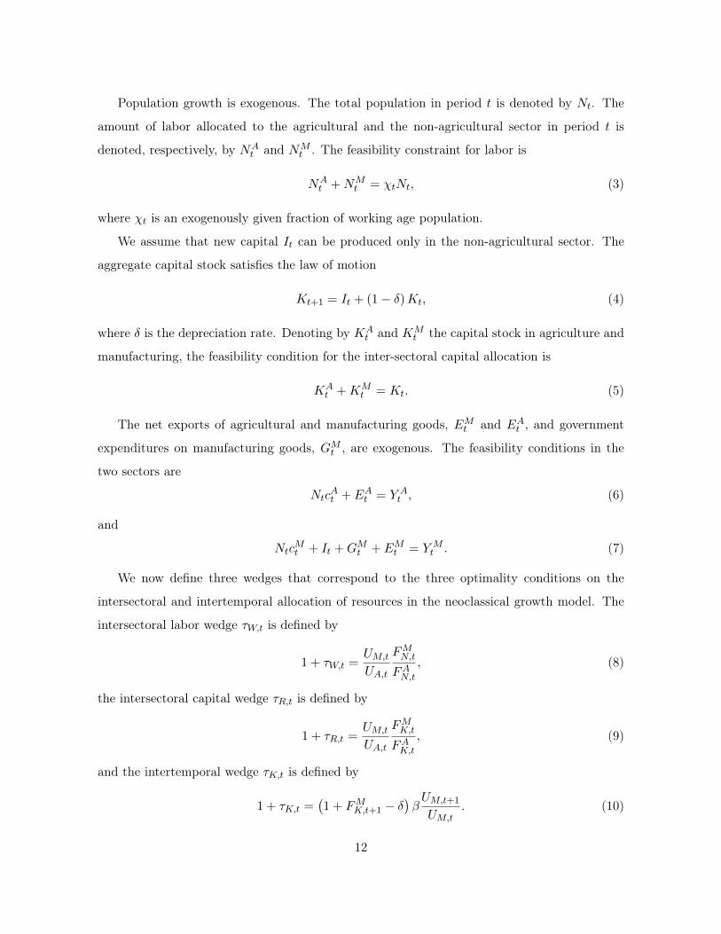
Population growth is exogenous. The total population in period t is denoted by Nt. The

amount of labor allocated to the agricultural and the non-agricultural sector in period t is

denoted, respectively, by NAt and NM

t . The feasibility constraint for labor is

NAt +NM

t = χtNt, (3)

where χt is an exogenously given fraction of working age population.

We assume that new capital It can be produced only in the non-agricultural sector. The

aggregate capital stock satisfies the law of motion

Kt+1 = It + (1− δ)Kt, (4)

where δ is the depreciation rate. Denoting by KAt and KM

t the capital stock in agriculture and

manufacturing, the feasibility condition for the inter-sectoral capital allocation is

KAt +KM

t = Kt. (5)

The net exports of agricultural and manufacturing goods, EMt and EAt , and government

expenditures on manufacturing goods, GMt , are exogenous. The feasibility conditions in the

two sectors are

NtcAt + EAt = Y A

t , (6)

and

NtcMt + It +GMt + EMt = YM

t . (7)

We now define three wedges that correspond to the three optimality conditions on the

intersectoral and intertemporal allocation of resources in the neoclassical growth model. The

intersectoral labor wedge τW,t is defined by

1 + τW,t =UM,t

UA,t

FMN,t

FAN,t, (8)

the intersectoral capital wedge τR,t is defined by

1 + τR,t =UM,t

UA,t

FMK,t

FAK,t, (9)

and the intertemporal wedge τK,t is defined by

1 + τK,t =(1 + FMK,t+1 − δ

)βUM,t+1

UM,t. (10)

12

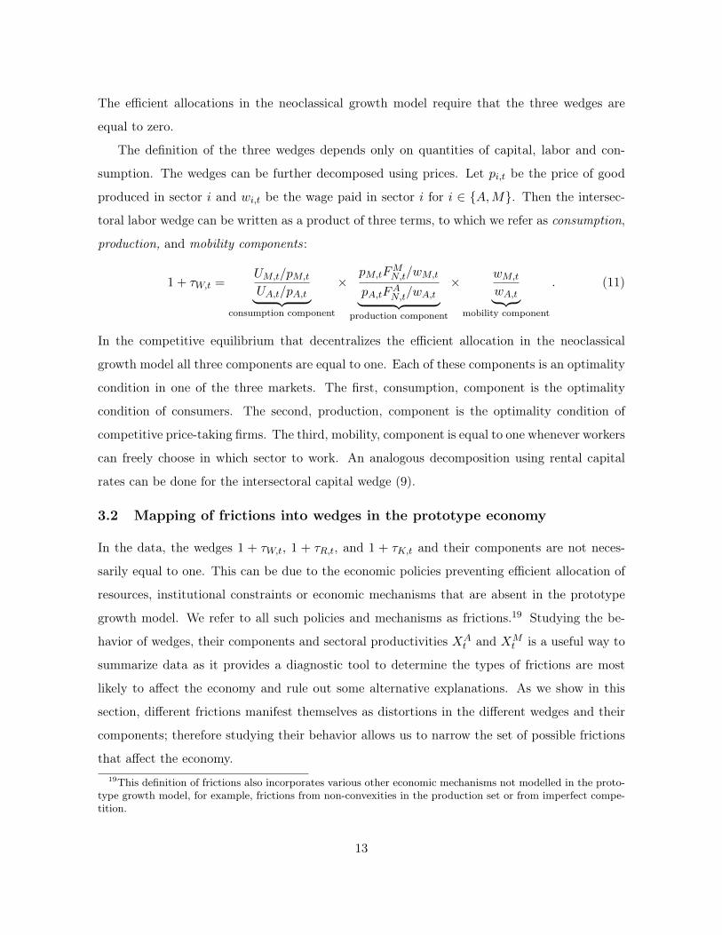
The efficient allocations in the neoclassical growth model require that the three wedges are

equal to zero.

The definition of the three wedges depends only on quantities of capital, labor and con-

sumption. The wedges can be further decomposed using prices. Let pi,t be the price of good

produced in sector i and wi,t be the wage paid in sector i for i ∈ A,M. Then the intersec-

toral labor wedge can be written as a product of three terms, to which we refer as consumption,

production, and mobility components:

1 + τW,t =UM,t/pM,t

UA,t/pA,t︸ ︷︷ ︸consumption component

×pM,tF

MN,t/wM,t

pA,tFAN,t/wA,t︸ ︷︷ ︸production component

×wM,t

wA,t︸ ︷︷ ︸mobility component

. (11)

In the competitive equilibrium that decentralizes the efficient allocation in the neoclassical

growth model all three components are equal to one. Each of these components is an optimality

condition in one of the three markets. The first, consumption, component is the optimality

condition of consumers. The second, production, component is the optimality condition of

competitive price-taking firms. The third, mobility, component is equal to one whenever workers

can freely choose in which sector to work. An analogous decomposition using rental capital

rates can be done for the intersectoral capital wedge (9).

3.2 Mapping of frictions into wedges in the prototype economy

In the data, the wedges 1 + τW,t, 1 + τR,t, and 1 + τK,t and their components are not neces-

sarily equal to one. This can be due to the economic policies preventing efficient allocation of

resources, institutional constraints or economic mechanisms that are absent in the prototype

growth model. We refer to all such policies and mechanisms as frictions.19 Studying the be-

havior of wedges, their components and sectoral productivities XAt and XM

t is a useful way to

summarize data as it provides a diagnostic tool to determine the types of frictions are most

likely to affect the economy and rule out some alternative explanations. As we show in this

section, different frictions manifest themselves as distortions in the different wedges and their

components; therefore studying their behavior allows us to narrow the set of possible frictions

that affect the economy.19This definition of frictions also incorporates various other economic mechanisms not modelled in the proto-

type growth model, for example, frictions from non-convexities in the production set or from imperfect compe-tition.

13

We now present several models of economic policies and frictions that are commonly dis-

cussed by economic historians in the context of the Russian economic experience of 1885-1940

and describe their mapping into wedges and their components. To simplify the exposition, we

focus on an economy without capital, with capital shares in both sectors set to zero. This

allows us to illustrate most mechanisms in a static model. We further set to zero exports and

government expenditures, normalize total population to 1 and assume that all of it is of working

age. We also set γA = 0, σ = αN,M = 1 and αN,A ≤ 1. These assumptions simplify notation

but are not essential for our arguments.

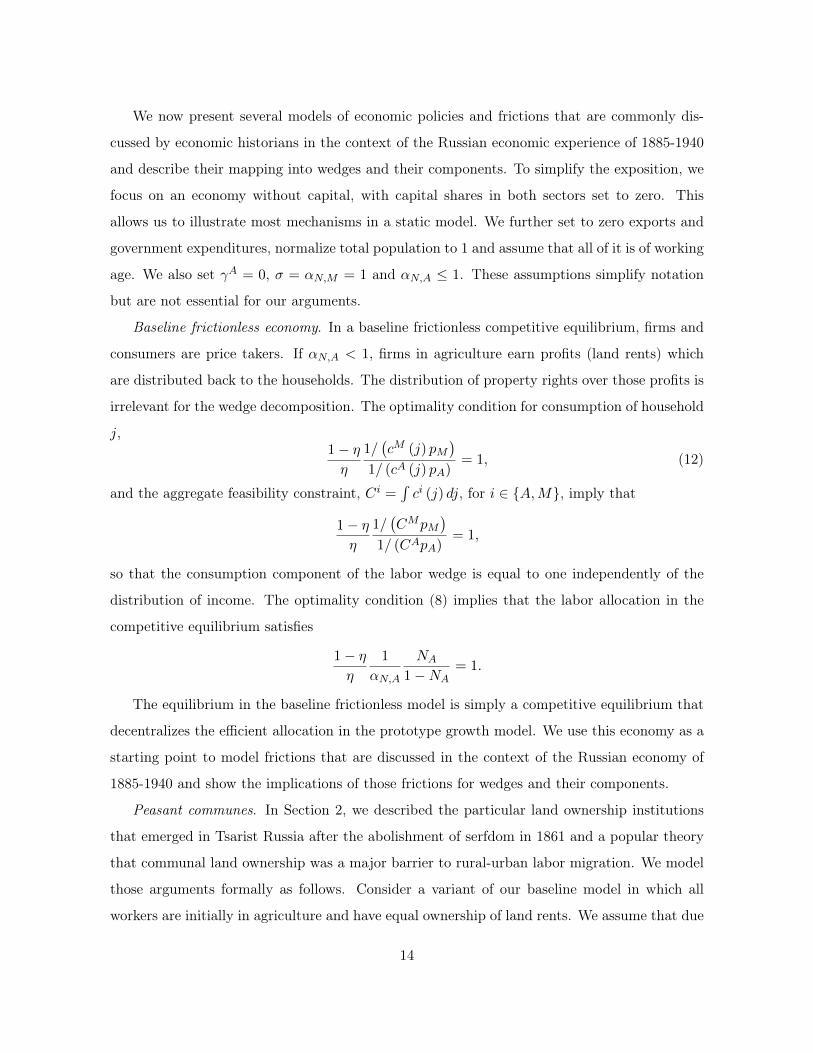
Baseline frictionless economy. In a baseline frictionless competitive equilibrium, firms and

consumers are price takers. If αN,A < 1, firms in agriculture earn profits (land rents) which

are distributed back to the households. The distribution of property rights over those profits is

irrelevant for the wedge decomposition. The optimality condition for consumption of household

j,1− ηη

1/(cM (j) pM

)1/ (cA (j) pA)

= 1, (12)

and the aggregate feasibility constraint, Ci =´ci (j) dj, for i ∈ A,M, imply that

1− ηη

1/(CMpM

)1/ (CApA)

= 1,

so that the consumption component of the labor wedge is equal to one independently of the

distribution of income. The optimality condition (8) implies that the labor allocation in the

competitive equilibrium satisfies

1− ηη

1

αN,A

NA

1−NA= 1.

The equilibrium in the baseline frictionless model is simply a competitive equilibrium that

decentralizes the efficient allocation in the prototype growth model. We use this economy as a

starting point to model frictions that are discussed in the context of the Russian economy of

1885-1940 and show the implications of those frictions for wedges and their components.

Peasant communes. In Section 2, we described the particular land ownership institutions

that emerged in Tsarist Russia after the abolishment of serfdom in 1861 and a popular theory

that communal land ownership was a major barrier to rural-urban labor migration. We model

those arguments formally as follows. Consider a variant of our baseline model in which all

workers are initially in agriculture and have equal ownership of land rents. We assume that due

14

to communal land ownership those rents are not transferable. If a peasant decides to work in

manufacturing he loses his rights to land rents, which are then redistributed equally among the

remaining agricultural workers. All other assumptions of the baseline model are unchanged.

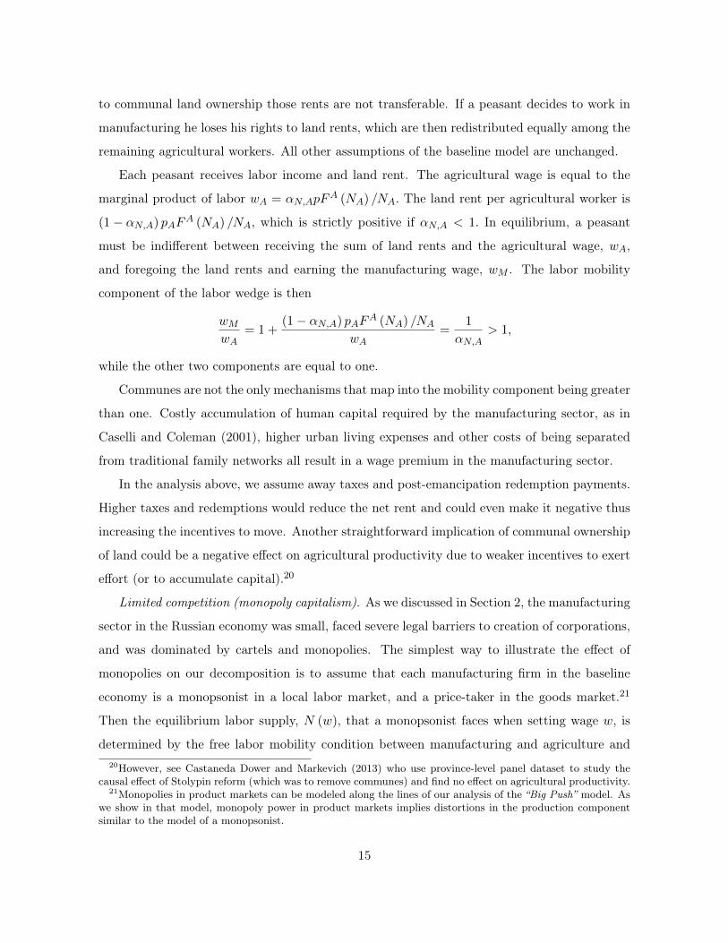
Each peasant receives labor income and land rent. The agricultural wage is equal to the

marginal product of labor wA = αN,ApFA (NA) /NA. The land rent per agricultural worker is

(1− αN,A) pAFA (NA) /NA, which is strictly positive if αN,A < 1. In equilibrium, a peasant

must be indifferent between receiving the sum of land rents and the agricultural wage, wA,

and foregoing the land rents and earning the manufacturing wage, wM . The labor mobility

component of the labor wedge is then

wMwA

= 1 +(1− αN,A) pAF

A (NA) /NA

wA=

1

αN,A> 1,

while the other two components are equal to one.

Communes are not the only mechanisms that map into the mobility component being greater

than one. Costly accumulation of human capital required by the manufacturing sector, as in

Caselli and Coleman (2001), higher urban living expenses and other costs of being separated

from traditional family networks all result in a wage premium in the manufacturing sector.

In the analysis above, we assume away taxes and post-emancipation redemption payments.

Higher taxes and redemptions would reduce the net rent and could even make it negative thus

increasing the incentives to move. Another straightforward implication of communal ownership

of land could be a negative effect on agricultural productivity due to weaker incentives to exert

effort (or to accumulate capital).20

Limited competition (monopoly capitalism). As we discussed in Section 2, the manufacturing

sector in the Russian economy was small, faced severe legal barriers to creation of corporations,

and was dominated by cartels and monopolies. The simplest way to illustrate the effect of

monopolies on our decomposition is to assume that each manufacturing firm in the baseline

economy is a monopsonist in a local labor market, and a price-taker in the goods market.21

Then the equilibrium labor supply, N (w), that a monopsonist faces when setting wage w, is

determined by the free labor mobility condition between manufacturing and agriculture and20However, see Castaneda Dower and Markevich (2013) who use province-level panel dataset to study the

causal effect of Stolypin reform (which was to remove communes) and find no effect on agricultural productivity.21Monopolies in product markets can be modeled along the lines of our analysis of the “Big Push” model. As

we show in that model, monopoly power in product markets implies distortions in the production componentsimilar to the model of a monopsonist.

15

decreasing returns to scale in agriculture,

w = wA = pAαN,A (1−N)αN,A−1 .

A monopsonist chooses the wage rate w to maximize its profit, pMN (w)−wN (w), taking the

labor supply equation as given. This implies that in equilibrium, the production component of

the labor wedge ispMF

MN /wM

pAFAN/wA= 1 + (1− αN,A)

NM

1−NM> 1,

which is a measure of markup over the monopsonist’s marginal cost. Therefore, monopoly

power maps into the production component of the intersectoral labor wedge.

Segmented consumer goods markets, rationing, stockouts. Various frictions in consumer

markets map into the consumption component of the labor wedge. Consider, for example, the

implications of a high cost of accessing markets for some peasants due to a poor transportation

network, as discussed in Section 2. We augment our baseline model by assuming that only a

fraction of all households can trade at prices pA and pM , while the remaining households are

located far from city markets and consume only the agricultural goods produced in their village.

Therefore, the optimality condition (12) applies only to the households in the first group. Let

x be the fraction of total agricultural consumption, CA, consumed by the households in the

first group. Then (12) implies that

1− ηη

1/(CMpM

)1/ (xCApA)

= 1,

and the consumption component of the labor wedge is

UM,t/pM,t

UA,t/pA,t=

1− ηη

xCApA + (1− x)CApACMpM

= 1 +1− ηη

(1− x)CApACMpM

> 1.

Other frictions in consumer markets have similar effects. For example, if demand for any good,

given prices pA and pM , exceeds supply, and the goods are rationed (as occurred, for example,

in Soviet Union in 1929-34), the ratio of marginal utilities of the two consumption goods may

systematically depart from the ratio of relative prices. The consumption component may be

greater or smaller than one depending on the relative prices set by the government.

Industrialization and collectivization. The Soviet government pursued a range of policies in

industry and agriculture often referred to as industrialization and collectivization. We briefly

comment on the implications of some of those policies for the production component of the

16

labor wedge. If the Soviet government starts with the Tsarist economy, distorted by monopolies

in manufacturing, and channels resources into that sector ignoring a monopolist’s optimality

condition, the markup in manufacturing, all other things being equal, should decrease. Specific

examples of such policies are explicit directions for state enterprises to meet ambitious output

targets or the “soft budget constraints” that subsidized state enterprises to expand employment

and investments.

The production component is a function of the relative markups in manufacturing and

agriculture, and it can be reduced both by decreasing markups in manufacturing and increasing

them in agriculture. As we discussed in Section 2, one popular view is that the movement

of labor into manufacturing was caused by the collectivization campaign that reduced the

standards of living of agricultural workers. A range of policies, such as the expropriation of

agricultural output and the creation of agricultural monopsony employers, the collective farms,

would lead to an increase in the wedge between the marginal product of labor in agriculture

and the income of agricultural workers, that maps into a higher markup in agriculture — hence

implying a lower production component.

Non-convexities, multiple equilibria and the “Big Push”.

One of the main explanations of Soviet industrialization is a “Big Push” theory. Big Push

assumes that due to coordination failure a decentralized market economy may get stuck in a

low-level “traditional” equilibrium while switching to a “modern” equilibrium with high level

of industrial output and standards of living requires a top-down effort. The standard way to

formalize this idea is to assume that modern technology involves increasing returns to scale.

Although our baseline framework uses constant returns to scale, it can also be applied to

the setting where the underlying technology has increasing returns. In the Appendix B, we

consider a well-known modern formalization of the “Big Push” idea by Murphy, Shleifer and

Vishny (1989) and apply our procedure to their setting, augmented with the agricultural sector.

Here we summarize the main insights of the model from the Appendix B and explain why they

hold in many other formalizations of the “Big Push” idea.

If the manufacturing sector is stuck in a bad equilibrium then capital and labor are utilized

inefficiently. As a result, the productivity of those factors is low. Any policy that shifts the

economy to a good equilibrium increases efficiency of factor utilitization. Therefore such policies

should lead to an increase in XM in our framework. In the Murphy, Shleifer and Vishny (1989)

17

model there is a bad equilibrium, where firms do not adopt efficient modern technologies due to

the aggregate demand externalities. There is also a good equilibrium, where the firms pay the

fixed cost of introducing modern technology and operate the technology at the efficient scale.

In the good equilibrium, firms capture some of the gains from aggregate demand spillovers due

to sufficient monopoly power. This implies that switching from the bad to the good equilibrium

also increases the labor wedge τW , in particular its production component.

4 Measurement of wedges in the data

In this section we discuss the data sources and the parameters that we use to measure sectoral

productivities, wedges (8), (9) and (10), and their components.

4.1 Parametrization

We draw on a large body of literature that used the prototype two-sector growth model of

Section 3.1 to study growth and structural transformation in various historical contexts.22

This literature has a broad consensus regarding the values for some of the key parameters.

The parameter η, that determines the long run share of agricultural expenditure in the total

consumption basket, is believed to be small, the elasticity of substitution between consumption

goods, σ, to be no greater than 1, and the labor shares in production, αA,N and αM,N , to be

quite large, at least 0.5 and possibly as high as 0.7 in manufacturing.

For the parameters σ, η, and γA we choose the values at the higher ends of the ranges

used in the literature; lower values would make our results stronger. In particular, we choose a

commonly used Stone-Geary specification σ = 1. We set the long run share of agricultural con-

sumption η to 0.15. We set subsistence parameter γA so that in 1885 the per capita agricultural

consumption is 25 percent above the subsistence level. We cannot choose a larger subsistence

level since in that case agricultural consumption in the data drops below the subsistence level

during the bad harvest of 1891. We base our technology specification on Caselli and Coleman

(2001), with the exception that we set the land share in manufacturing to 0 rather than 0.06.

For the fraction of the labor force in the population, we set χt = 0.53 for 1885-1913 (based22For example, Caselli and Coleman (2001), Buera and Kaboski (2009, 2012a,b), Herrendorf, Rogerson and

Valentinyi (2013) applied this model to the economic experience of the U.S. in the 19th and 20th centuries,Stokey (2001) to the industrial revolution in England, Hayashi and Prescott (2008) to Japan in the 20th century.

18

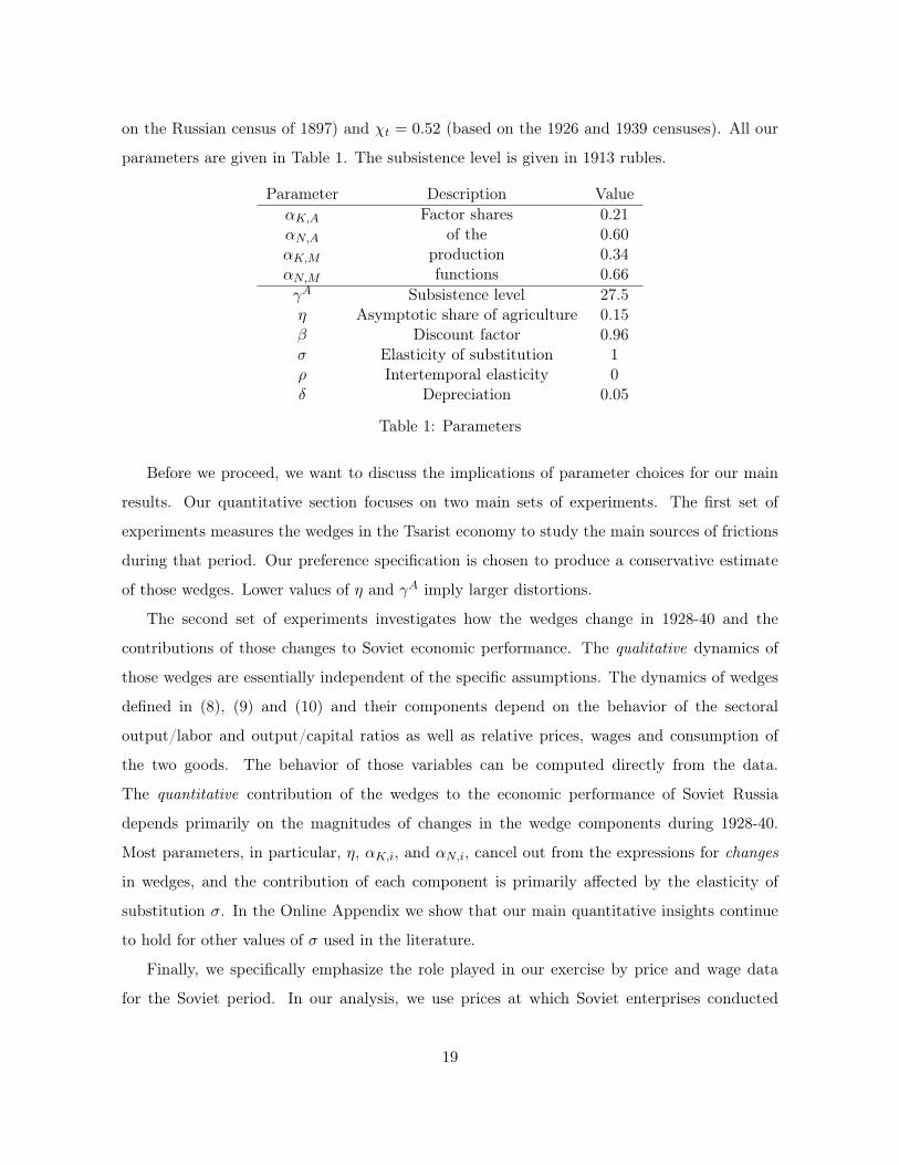
on the Russian census of 1897) and χt = 0.52 (based on the 1926 and 1939 censuses). All our

parameters are given in Table 1. The subsistence level is given in 1913 rubles.

Parameter Description ValueαK,A Factor shares 0.21αN,A of the 0.60αK,M production 0.34αN,M functions 0.66γA Subsistence level 27.5η Asymptotic share of agriculture 0.15β Discount factor 0.96σ Elasticity of substitution 1ρ Intertemporal elasticity 0δ Depreciation 0.05

Table 1: Parameters

Before we proceed, we want to discuss the implications of parameter choices for our main

results. Our quantitative section focuses on two main sets of experiments. The first set of

experiments measures the wedges in the Tsarist economy to study the main sources of frictions

during that period. Our preference specification is chosen to produce a conservative estimate

of those wedges. Lower values of η and γA imply larger distortions.

The second set of experiments investigates how the wedges change in 1928-40 and the

contributions of those changes to Soviet economic performance. The qualitative dynamics of

those wedges are essentially independent of the specific assumptions. The dynamics of wedges

defined in (8), (9) and (10) and their components depend on the behavior of the sectoral

output/labor and output/capital ratios as well as relative prices, wages and consumption of

the two goods. The behavior of those variables can be computed directly from the data.

The quantitative contribution of the wedges to the economic performance of Soviet Russia

depends primarily on the magnitudes of changes in the wedge components during 1928-40.

Most parameters, in particular, η, αK,i, and αN,i, cancel out from the expressions for changes

in wedges, and the contribution of each component is primarily affected by the elasticity of

substitution σ. In the Online Appendix we show that our main quantitative insights continue

to hold for other values of σ used in the literature.

Finally, we specifically emphasize the role played in our exercise by price and wage data

for the Soviet period. In our analysis, we use prices at which Soviet enterprises conducted

19

their transactions and measures of relative income for urban and rural workers. Our analysis

does not require an assumption that the economic agents can freely make decisions given those

prices. As we emphasized in Section 3.2, the additional distortions that the command economy

introduces given those prices are captured by the components of the wedges that we measure.

4.2 Data

In this section, we briefly discuss the construction of the data (see Appendix A for the com-

prehensive description of our data sources). The main source of economic data for output,

consumption, and investment for Russia in 1885-1913 is Gregory (1982). Gregory compiled

data on the net national income and its components using a variety of historical sources, most

of them based on the official Tsarist statistical publications. His data are sufficiently disaggre-

gated and allow us to construct the series for consumption and investment in the agricultural

and non-agricultural sectors and to use a perpetual inventory method to impute capital stock

in each sector. Gregory provides data on the sectoral composition of value added for selected

years, and we interpolate between them. Employment is constructed using the census of 1897

and Gregory’s estimates of the sectoral employment growth rates over different sub-periods of

1885-1913.

For relative prices we use the price deflator implied by Gregory’s series. Our wage data are

from Strumilin (1960, 1982), which in turn is based on administrative records of the Tsarist

period. For agricultural wages we take the average annual wages of a male employee (batrak)

hired on a year-long contract. For manufacturing wages we take the average annual wages of

male factory workers.

Our main source of the Soviet economic data on quantities is from the comprehensive work of

Moorsteen and Powell (1966) which is widely used by Western economic historians. Moorsteen

and Powell use official Soviet data to construct sectoral outputs, capital stocks, and value added

according to Western definitions. To construct the sectoral employment shares, we use the 1926

and 1939 censuses and Soviet employment records.

We use two versions of price series to construct the relative prices. For our baseline spec-

ification, we use wholesale prices at which Soviet companies conducted transactions. We also

use indices of retail prices in private markets. Both price indices are from Allen (1997).

In order to determine relative wages, we use Allen’s (2003) estimates of farm and non-farm

20

consumption per head in 1928-1939.23 For this, he measures the in-kind income in private

market prices, adds cash income and subtracts taxes. He assumes that all income is spent on

consumption, which is essentially equivalent to our notion of wages.

One natural concern is whether the official Soviet output series, on which Moorsteeen and

Powell base their analysis, and on which most subsequent research builds, are reliable. The

opening of the Soviet archives allowed historians to re-estimate production data using inter-

nal documents (Davies et al., 1994, pp. 115-117); these updated numbers turned out to be

broadly consistent with the estimates of by Moorsteen and Powell. According to Allen (2003,

p. 212), “Did the Soviets really produce as many tons of steel or pairs of shoes as they claimed?

Many Western scholars have investigated this question, however, and the consensus is that the

published Soviet figures for output were basically reliable”. The recent archival work and the

analysis of Soviet production data using contemporary American input-output relationships

did not uncover any significant inconsistencies.

Since the role of government changed dramatically between 1913 and 1928, we define gov-

ernment purchases narrowly as military spending. This definition also allows us to calculate

the contribution of military buildup before WWII to structural change. We count all other

government spending as non-agricultural consumption.

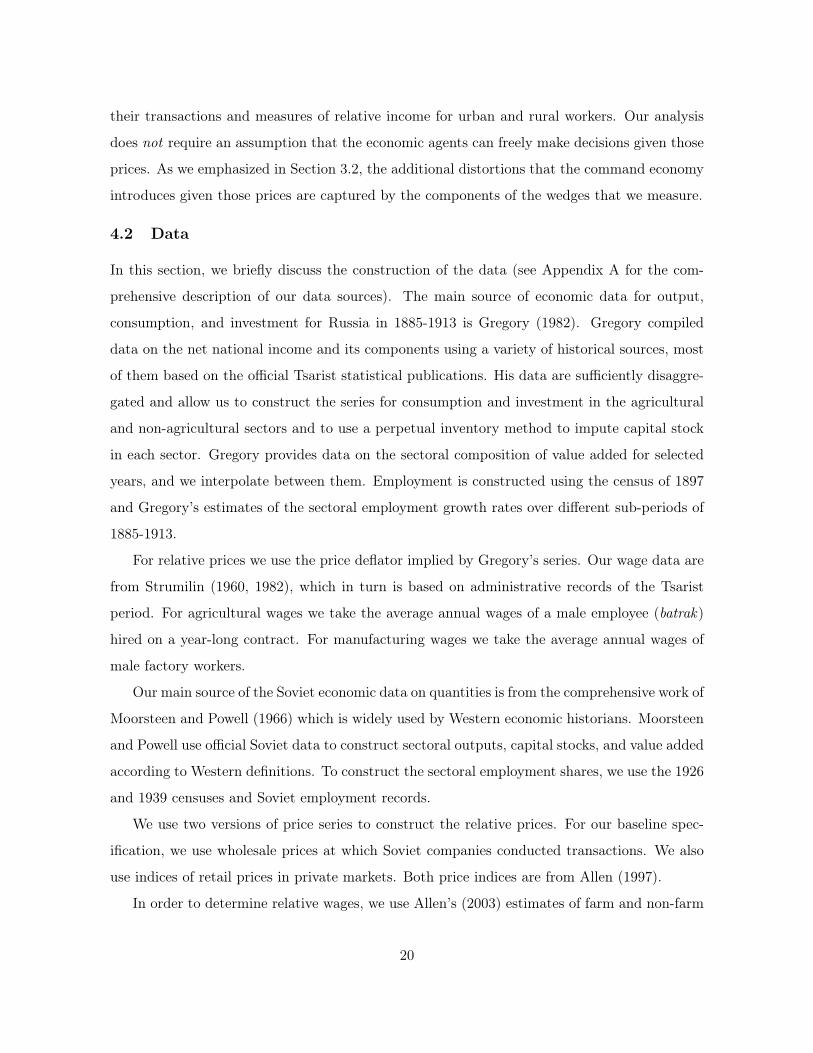
Figure 1 presents the sectoral data for the Tsarist and the Soviet period.

Figure 1: Aggregate economic indicators in Russia in 1885-1940.

The Russian economy in 1885-1913 grew at 1.8 percent per annum in per capita terms.23We do not use the wage data directly as a large fraction of agricultural income was in kind.

21

However, the economy did not experience structural transformation from agriculture. The

primary occupation for about 85 percent of the working-age Russian population was agriculture

in 1885, and this fraction declined very slowly, to 82 percent in 1913. The role of agriculture in

the value added was also very important, with about 54 percent of GDP produced in agriculture

in 1885, declining only to 47 percent in 1913. Figure 1 measures the share of value added in

agriculture in 1913 prices to isolate the effect of changes in quantities.

The level of GDP per capita and the structural composition of the Russian economy in

1928 were approximately the same as they were in 1913.24 In 1928-1940, growth in real GDP

(measured in 1913 rubles) is very rapid but it starts from a low base and by 1940 GDP per

capita is just above the pre-1913 trend. GDP per capita should also be interpreted with caution

due to the so-called “Gerschenkron effect”. We report GDP per capita in 1913 prices, at which

point the manufacturing sector was relatively small and the relative prices of manufacturing

goods were high. Since manufacturing output grew faster than agricultural output after 1928,

the baseline prices of early years are particularly favorable to show high rates of GDP growth.

The structural transformation was much faster in 1928-1940 than in 1885-1913. In particu-

lar, the labor force in manufacturing almost tripled during the 1928-1940 period (from 10.5 to

30.2 million workers, or from 13 to 34 percent of total employment).

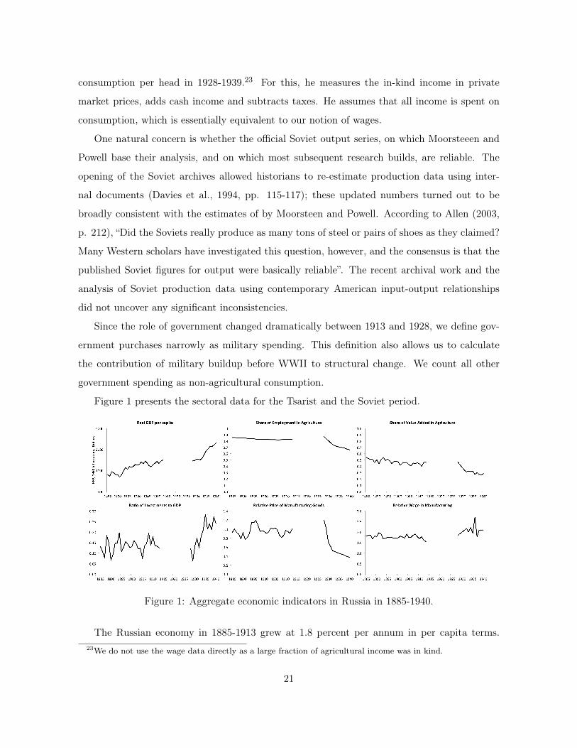
5 Wedge decomposition

Figure 2 presents sectoral productivities XMt , XA

t and the wedges 1+τW,t, 1+τR,t and 1+τK,t.

The dashed lines are the Tsarist trend growth rates for XMt and XA

t and the average values of

the quantity wedges in 1885-1913 (with the exclusion of the famine years in the early 1890s)

for a comparison with the frictions in the Soviet economy.24We do not report the data for Tsarist Russia during World War I (1914-1917) or for the period between the

February Revolution of 1917 and 1927. This period covers the October (Bolshevik) Revolution, the Civil War,War Communism, and the New Economic Policy (NEP). This is because the availability and quality of data donot allow us to build a dataset comparable in quality to the one we construct here. Even though Markevichand Harrison (2011a) provide many time series for this period, there are still no data for capital. That is whywe are not able to estimate TFP and wedges for those periods.

22

Figure 2: Sectoral TFPs (in logarithms) and Wedges in Russia in 1885-1940.

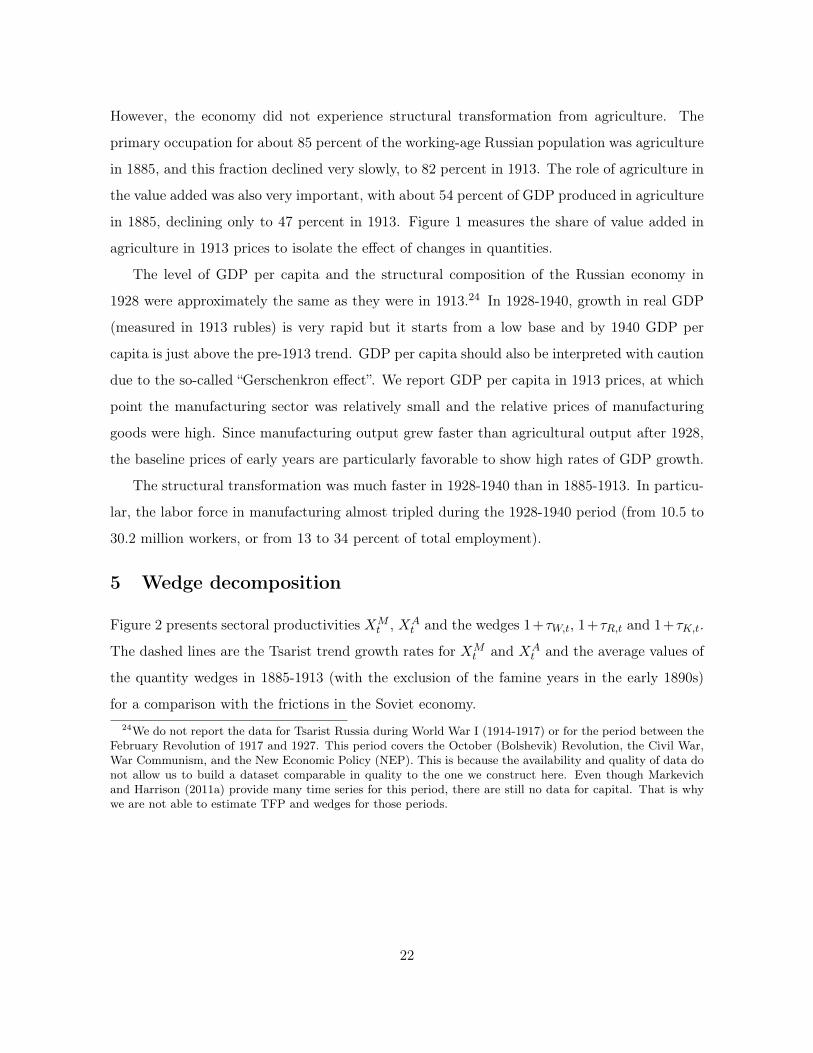
Figure 3 shows the decomposition of the wedges 1+τW,t and 1+τR,t into their components.

Since there are no data on the sectoral capital rental rates, we compute only a product of the

production and mobility components of the intersectoral capital wedge. In our discussion of the

results we mainly focus on the labor wedge decomposition since we can measure its components

more precisely.

Figure 3: Components of intertemporal labor and capital wedges in Russia in 1885-1940.

5.1 Wedges in 1885-1913 (Tsarist Russia)

The most important observation regarding the wedges in this period is that the distortions

to the intersectoral allocation of factors of production in Tsarist Russia are very high. The

average value of the labor wedge during 1885-1913 is 14, which is equivalent to an ad valorem

tax of 1,300 percent on moving labor from the agricultural to the manufacturing sector. From

the standpoint of the neoclassical growth model, there are large efficiency gains that could be

23

achieved by reallocating labor away from agriculture. All three components of the labor wedge

are sizable but their relative importance is quite different.

The production component of the labor wedge is the most significant one, accounting for

half of the overall wedge.25 It suggests that frictions in the production process that cause

under-utilization of labor in manufacturing were particularly severe in Tsarist Russia. High

values of the production component are consistent with monopoly power in product or labor

markets (see our discussion in Section 3.2). Therefore, our decomposition is consistent with

the view that cartels, monopolies, and various administrative barriers to creating and running

corporations were an important reason for the low share of manufacturing production in Russia

before WWI.

Why is the production component large? Our decomposition suggests that markups in

non-agricultural production were significant. To check this hypothesis more directly, we calcu-

lated the total labor bill in a subset of the non-agricultural sector for which the best data are

available – industrial factories.26 Gregory (1982) reports that the value added in factories was 3

billion rubles in 1913, and employment records show that factories employed 2.3 million people

(Gregory, 1972). Factory surveys during the Tsarist period show that the average annual wage

in factories was 257 rubles in that year (Allen, 2003, Strumilin, 1960), which implies that the

total wage bill was less than 20 percent of the total factory value added. Standard estimates

of the labor share in production are in the range of 60-70 percent, which implies a markup of

3-3.5, remarkably close to the average markup of 3.5 that we obtain through our decomposition.

The labor mobility component is substantial but it is the smallest of the three components,

and its relative significance further falls after 1895. Its average value of 1.8 implies that manu-

facturing wages are 80 percent higher than agricultural wages. Higher wages in manufacturing

are a common historical phenomenon, and such factors as costly skill acquisition or higher ur-

ban living expenses can partially account for that.27 The agricultural policies in Tsarist Russia25The average value of the production component was 3.5, therefore it accounted for ln(3.5)/ln(14)=47 percent

of the total labor wedge. The consumption component and the mobility component accounted for 33 and 21percent, respectively.

26According to Gukhman (1926, p. 251), factories accounted for 44 percent industrial employment in 1913and 99 percent of their employment were hired workers. The rest of the industrial sector were small businessesor artisans (“kustars”) not covered by the industrial statistics. By using the wage data from the large factorieswe essentially assume that the opportunity cost of small business owners’ labor was similar to the wages in thelarge factories.

27See Caselli and Coleman (2001) for the emphasis on skill composition and its implications for the behaviorof prices and wages in the neoclassical growth model. Allen (2003) discusses the importance of skill acquisition

24

that discouraged labor mobility (see our discussion of communes in Sections 2 and 3.2) are

the residual of this component, once wages are adjusted for those factors. Therefore, policies

that discourage labor mobility are unlikely to play an important role in slowing labor reallo-

cation from agriculture to manufacturing. Contrary to the views of Lenin, Gerschenkron and

many others, Russian communes do not appear to be among the main barriers to structural

transformation.28

The consumption component of the labor wedge is sizable. This is consistent with the

evidence that different regional markets were poorly integrated and that many Russian farmers

were “subsistence-oriented”, producing only a small fraction of their income for commercial

sale. As we showed in Section 3.2, costly access to centralized markets maps into a positive

consumption component in our decomposition.29

5.2 Wedges 1928-1940 (Soviet Russia)

The analysis of Figures 2 and 3 reveals two broad patterns during 1928-40. Productivity

performs poorly in both sectors, and both the labor and the capital intratemporal wedges fall

relative to their average Tsarist levels. The drop in the labor wedge is fully accounted for by

in the Russian economy. The only wage series we have for manufacturing workers that contains informationabout skills is the time series for construction workers in St Petersburg from Strumilin (1960). The wages foran unskilled construction worker (chernorabochij ) in that data set are about 50 percent higher than the averageagricultural wages in the European provinces of the Russian empire.

28This finding is consistent with the recent work by economic historians who used the available micro-datato study the causal effect of communal land holdings on rural-urban migration. Crisp (1978, p. 323-325) andGregory (1994) argue that communal restrictions on rural-urban migration were not a binding constraint forindustrialization. Borodkin, Granville, and Leonard (2008) use time series evidence for the Saint Petersburgregion and Nafziger (2010) analyzes a household-level dataset of villages in the Moscow province to reach similarconclusions.

29See also Spulber (2003, p. 101) for various administrative measures that hampered domestic trade. Spulber(p. 111) gives the statistics on how inefficient and limited the Russian railroad system was. For example, atthe end of 1913, Russia had only 1/12th of railroad coverage in terms of kilometers of railway per 100 squarekilometers of territory, compared to Great Britain, Ireland and Germany. Spulber (p. 76) concludes that “themajor part of the peasant farms constituted a subsistence sector, and the limited rest, a commercialized sector”.Metzer (1973, 1976) compares the contribution of railroads to the Russian economic growth and concludesthat it was much smaller than in the US. Gregory (1994) and Metzer (1974) argue that expansion of railroadsdid contribute to the spatial integration of commodity markets and reduction in interregional dispersion ofagricultural prices. While the interregional dispersion decreased by the end of the period, on average duringthe period market integration was still low: e.g. the wheat price differential between Moscow and Rostov was40 percent by the end of the period (Metzer, 1974, Appendix Table II). Also, Metzer’s evidence applies only toselected cities, most of them ports so prices there should have converged as they exported grain to the globalmarket; Russian grain exporting cities were well integrated into the global agricultural trade (see Goodwin andGrennes (1998) who show that wheat prices in Russian ports were correlated with prices in New York and inEngland and that the gap between prices in Odessa and international prices was low). This does not contradictour theoretical argument which refers to the lack of integration between peasants and cities which was stillimportant as majority of grain harvest was not commercialized (Metzer, 1974, Table 6).

25

the drop in its production component. By 1935, this component reaches the level close to one

as in the frictionless neoclassical benchmark. The mobility component remains at the average

Tsarist level. The consumption component increases, especially after 1933.

Note that both the intersectoral distortions and sectoral productivities are at a local mini-

mum in 1933 coinciding with the peak of the economic disruption, including famine in several

parts of the country. The behavior of wedges and productivity in 1928-1935 can be understood

by considering the effect of collectivization and industrialization in those years. The collec-

tivization policy starting from 1928 dramatically reduced prices paid to peasants for agricul-

tural goods, introduced state-run collective farms, and expropriated the “surplus” agricultural

output. These policies resulted in a significant fall in the agricultural production, the famine

in the countryside, and the flight of the peasants to the cities. The industrialization policy in

manufacturing substantially expanded investments in the non-agricultural sector, particular in

the heavy industry. As we have discussed in Sections 2 and 3.2, these policies have resulted

in a reduction in capital and labor wedges, and a decrease in sectoral productivities. In what

follows, we consider the impact of collectivization and industrialization on individual wedges

and their components.

One of the most salient results is the significant decrease in the production components

between 1928 and 1940. The production component is the ratio of markups pj,tFjN,t/wj,t in

the non-agricultural and the agricultural sectors. We can further decompose what part of

the decrease in the production component is driven by the numerator (the markup in the

non-agricultural sector) and by the denominator (the markup in agriculture). Let us denote

∆z = zt′′ − zt′ , the change in variable zt between years t′ and t′′. We have

∆ ln (production component) = ∆ ln (markup non-agr)−∆ ln (markup agr) .

In our data both terms are positive so that both the reduction in the markup in manufacturing

and the increase in the markup in agriculture contributed to the decrease in the production

component. Quantitatively, the decrease in the markup in the non-agricultural sector plays

a much larger role; it accounts for 84 percent of the decrease in the production component

between 1928 and 1939.

In the Tsarist economy, the high level of the production component was likely to be driven

by the market power of monopolies in the manufacturing sector. These firms maximized their

26

profits by reducing their output below the socially optimal level. Any policy that encourages

manufacturing producers to expand output should on the margin reduce the markup in the

manufacturing sector, reduce the production component of the labor distortion, and reallocate

labor from agriculture to manufacturing. Removal of entry barriers and promotion of competi-

tion are examples of such policies in competitive economies. In the Soviet economy, the central

government incentivized enterprise managers to achieve ambitious production targets rather

than to maximize profit, and channeled resources into industry, which also led to an expansion

of industrial output, to reallocation of labor, and to a reduction in the production component

of the intersectoral labor wedge. Soviet agricultural policies also contributed to the reduction

of the production component as an increase in monopsony power of the state farms over the

peasants resulted in higher markups in agriculture, but their effect was small.

In Figure 2 we compare the performance of agricultural and non-agricultural TFPs during

1928-40 to their respective Tsarist trends. The behavior of sectoral TFPs is consistent with a

view that the Soviet economy, although successful in reallocating resources towards manufac-

turing, failed to provide the right conditions for efficient utilization of those resources within

each sector. The non-agricultural TFP was falling throughout the whole period. The agricul-

tural TFP fell drastically in 1928-1933. Even though the agricultural productivity recovered

later, it remained below the Tsarist trend. While a portion of the productivity drop can be

accounted for by other factors such as the large inflow of relatively inexperienced, low-skill

workers into manufacturing, the poor performance of agricultural productivity and output are

particularly illustrative. Davies et al. (1994) trace the drop in the agricultural output to sev-

eral factors. They argue that the state exaction of grain from peasants on its own created

dramatic disruptions to agricultural production by reducing incentives to work on collectivized

land, by disrupting the system of crop rotation, and by a drastic fall in the number of draught

animals. Moreover, the dekulakization campaign led to exile and execution of the most skilled

and entrepreneurial farmers.

Our findings are inconsistent with the predictions of “Big Push” theories that sweeping state

investments should increase productivity in the manufacturing sector and increase the labor

wedge (see Section 3.2). We observe exactly the opposite. The labor wedge significantly de-

creased. TFP fell in both sectors during the main phases of industrialization and collectivization

and remained below Tsarist trends in most years.

27

Our results are also not consistent with the view that collectivization policies played a

major role in changing intersectoral distortions: we show that the decrease in the production

component was mostly driven by the reduction of markups in the non-agricultural sector rather

than by the increase in markups in argiculture. At the same time, our findings lend support

to the view that policies that encouraged expansion of manufacturing, e.g., through the use

of explicit output targets, “soft budget constraints”, etc., significantly affected intersectoral

allocation of resources.

5.3 Discussion

In this section we discuss which features of the data drive our results. We focus on what

we view as our two main findings: (1) the labor wedge and, in particular, its production

component, decreased significantly, and (2) manufacturing TFP performed poorly between

1928 and 1940. We also explain why during this time period the intertemporal wedge changed

little despite a large increase in the investment to output ratio during this time period, and

why the consumption component increased.30

All these results characterize the rates of change of distortions. We show below that these

rates can be written in terms of directly measurable economic aggregates in a way that ei-

ther does not include any parameters of the model at all, or includes only a small number

of parameters. This implies that our broad conclusions should be robust to a wide range of

model specifications. We demonstrate this point explicitly in the Online Appendix where we

re-calculate wedges and their components and quantify their effect for a number of alternative

parameterizations of our model. Russian economic data in the late 19th – early 20th century

are imperfect, and there is a certain amount of measurement error in the time series. We discuss

alternative estimates of the key elements of our decomposition and argue that they are broadly

supportive of our conclusions.

5.3.1 Non-agricultural productivity in 1928-40

We showed in Figure 2 that non-agricultural productivity fell during 1928-40. To understand

what drives this decline, we write the rate of change in TFP as

∆ lnXM = ∆ lnYM −(αN,M∆ lnNM + αK,M∆ lnKM

).

30Section 3 in the Online Appendix provides comparison of wedges and productivities in 1928 and 1913.

28

In our data, output YMt grew rapidly and increased between 1928 and 1939 by a factor of

2.4.31 The non-agricultural employment and capital stock increased even faster: NMt increased

by a factor of 2.9, and KMt increased by a factor of 3.8. Therefore, as long as we assume that

production function in manufacturing has constant returns to scale (αK,M + αN,M = 1), we

should find that XMt performed poorly for any choice of the factor shares.

Rapid growth in labor and capital in the non-agricultural sector has been well documented.

The estimates of non-agricultural labor force are available from the censuses of 1926 and 1939

and from administrative records during 1928-40, and these numbers are broadly consistent

with each other. The data on capital stock are less reliable (we discuss them in more details

in Section A.1) but there is little doubt that capital stock in non-agricultural sector increased

significantly during this period, most likely even faster than the non-agricultural employment.

The estimates of YM have been controversial, in part because the choice of the base-year

to calculate the price deflators affects conclusions about the growth rate of the output due

to large changes in relative prices during this time period. Our estimates, however, are well

within the range available in the literature. Davies et al. (1994, Table 24) survey the existing

estimates of the annual growth rates of industrial production and show that they range from

7.1 to 13.6 percent. Allen (2003, Table 5.4) estimates the growth rate of industrial output to be

11 percent. In our dataset, YM which includes both industrial production and services, grew

by 8.7 percent, and there is little doubt that the growth rate in services was much slower than

the growth rate in manufacturing (see also Allen 2003).

5.3.2 The labor wedge and its production component

We find that the labor wedge was high in the Tsarist economy. This finding is driven by the

fact that we adopted a preference parameterization frequently used in the literature. In the

late 19th-early 20th century the Russian economy was much more agricultural than economies

of other countries at similar stages of development. Therefore, the intersectoral wedges would

generally be high in Russia if model parameters are chosen at levels consistent with experiences

of those countries. The rapid structural change during 1928-1940 then should imply a decrease

in these wedges.

One of our central findings is that the decrease in the intersectoral labor wedge is driven31Since Soviet borders changed in 1940, we focus on the comparison between 1928 and 1939 to avoid additional

data issues.

29

primarily by the rapid decrease in its production component. The rate of change in the pro-

duction component is not a function of model parameters and can be written as a sum of rates

of change of the following macroeconomic time series:

∆ ln (production component) = ∆ ln

(pMpA

)+ ∆ ln

(YM/NM

Y A/NA

)+ ∆ ln

(wAwM

). (13)

In our dataset, all three terms on the right hand size of this expression decrease between 1928

and 1939 and account for 74 percent, 17 percent and 9 percent of the fall in the production

component, respectively.

The fall in all three components is consistent with findings in a number of studies of the

Soviet economy during this period. The large fall of the relative prices pM,tpA,t

in Russia is widely

documented and has been studied at least since Gerschenkron (1951). In our calculations we

use wholesale industrial and agricultural prices from Allen (1997) as a proxy for the producer

prices that are needed for our calculations, which show that pM,tpA,t

dropped between 1928 and

1939 by a factor of 3.1.

The second term on the right hand side of equation (13) is negative because output per

worker in agriculture grew faster than output per worker in non-agriculture. As we already

discussed, the evidence points to a likely fall in non-agricultural output per worker between

1928 and 1939. At the same time, our data show that agricultural output per worker increased

by about 30 percent. This increase comes from the fact that agricultural output was higher in

1939 than in 1928 while agricultural employment was lower. Both higher agricultural output

and lower agricultural employment are consistent with the literature. For example, Davies et

al. (1994, Tables 18 to 22) show that agricultural production in physical units increased in

almost all categories. Allen (2003, table 5.4) argued that agricultural value added increased

by 10 percent. At the same time, rapid reallocation of labor force to manufacturing implies

that agricultural employment was lower in 1939 than it was in 1926; this is confirmed by the

censuses of 1926 and 1939.

The least information is available about the behavior of real earnings in agriculture and

non-agriculture. We are only aware of the estimates in Allen (2003, table 7.4) that relative

consumption per head of a farm worker to a nonfarm worker decreased by about 12.5 percent

between 1928 and 1939. The observation that the relative standards of living in agriculture fell

is also consistent with the introduction of passports and the urban registration system meant

30

to slow the flow of agricultural workers into the cities.

5.3.3 The consumption component and the intertemporal wedge

In this section we explain why our decomposition shows no changes in the intertemporal wedge

τKt during 1928-1939, while at the same time we observe doubling of the investment to output

ratio and an increase in the consumption component, especially after 1933. These three facts

are closely related.

The intertemporal wedge (10) is a combination of the marginal product of capital in the non-

agricultural sector and of the growth rate of non-agricultural consumption. High investment

rates lead to a fall in the marginal product of capital. At the same time, the growth rate of

non-agricultural consumption also slowed down, offsetting the decrease in the non-agricultural

marginal product of capital. The slow growth rate of non-agricultural consumption results not

only in a flat intertemporal wedge but also in an increase in the consumption component of the

labor wedge. In particular, a rapid fall in relative prices of manufacturing goods together with

an increase in total output imply that a much faster growth rate of cM,t should be optimal in

the absense of a change in consumption distortions. Hence, a higher consumption component is

needed to reconcile the relative price changes with the low level of manufacturing consumption.

The flat intertemporal wedge is consistent with rising investment to GDP ratios because

the optimal investments in the neoclassical model are determined not only by the intertem-

poral wedges but also by the expectations of the future behavior of the intersectoral wedges.

As we see in Figure 3, the consumption component increases. This rise in the consumption

component lowers the growth rate of non-agricultural consumption (and increases the growth

rate of marginal utility), especially in the second half of the period.

The rise in the consumption component after 1933 is not caused by rationing: by all ac-

counts, there were no overt deficits in state stores after 1937 and consumers could buy retail

goods more or less freely. Rather, the relative prices that consumers faced in those stores be-

haved differently from the relative producer prices: the relative wholesale prices of industrial

goods fell 50 percent faster than the relative retail prices (Allen 1997). Let us denote qA,t and

qM,t the retail prices for agricultural and non-agricultural goods, respectively. We can rewrite

the rate of change in the consumption component as

∆ ln (consumption component) = ∆ ln

(UM/qMUA/qA

)+ ∆ ln

(qM/qApM/pA

).

31

The difference in the rate of change in wholesale and retail prices ∆ ln(qM/qApM/pA

)explains 85

percent of the change in the consumption component.

The likely explanation of this behavior is the distortion of allocations within the non-

agricultural sector. It is widely acknowledged that Soviet industiralization policies favored

heavy industry at the expense of the consumer goods industry and services. Such policies

should imply that prices of goods produced by heavy industry should fall faster than prices

of consumer goods and services. As a result, the ratio qM,t/qA,tpM,t/pA,t

increases, lowering the growth

rate of non-agricultural consumption, cMt .

To summarize, the incentives to increase investment can be provided by changing either

the intertemporal prices, which corresponds to a gap between interest rates and the marginal

product of capital, or by changing the intra-sectoral prices that consumers face over time (as

the latter affect the composition of consumption). The Soviet government pursued policies that

affected investment through the second channel.

6 Counterfactual analysis

In addition to inferring the wedges from the macroeconomic data, our framework allows us to

construct counterfactual scenarios. In this section we describe the methodology of our coun-

terfactual analysis and carry out three quantitative exercises. First, we compare the actual

Soviet economic data to a counterfactual based on extrapolation of the pre-1913 trends. We

decompose the difference between the actual state of the Soviet economy in 1939 and the coun-

terfactual into contributions of individual wedges and their components. The second exercise is

similar but instead of comparing 1939 levels, we analyze the changes over the 1928-1939 period.

Both exercises point to the key role of the production component. This is why we carry out the

third exercise where we project the evolution of the Tsarist economy without the production

component of the labor wedge.

6.1 Methodology

Let us consider any T -period sample D =

cjt , Y

jt ,K

jt , N

jt , wj,t, pj,t

j∈A,M

, It

Tt=1

. This

sample allows computing intersectoral wedges and their components for T periods, sectoral

32

productivities in T periods and the intertemporal wedge in T − 1 periods. Let us denote

κT = IT /YMT (14)

and let Ω be a vector that consists of production, consumption, mobility components in both

sectors in T periods, sectoral TFPs, net exports, government spending and demographic vari-

ablesXAt , X

Mt , EAt , E

Mt , Gt, Nt

Tt=1

,τKtT−1

t=1as well as K1 and κT . Equations (2)-(11) and

(14) define a one-to-one correspondence between D and Ω. This implies that if we know dis-

tortions Ω generated by data D, we can recover D.

Equation (14) provides a simple way to capture expectations. The optimal level of invest-

ment in the last period, κT = IT /YMT , is determined by expectations of the future evolution

of the macroeconomic variablesXAt , X

Mt , EAt , E

Mt , Gt, Nt, τ

Kt−1, τ

Wt , τRt

∞t=T+1

. Any given in-

vestment to manufacturing output ratio κT is consistent with a continuum of different future

paths of these variables. However all those paths affect variables before period T only through

κT – holding κT constant, distortions in the first T periods uniquely pin down allocations in

the first T periods.

How much a difference between the data D and any counter-factual experiment D′ is ac-

counted for by the change in any given distortion (Ω vs Ω′)? Since any counterfactual sample

D′ is uniquely associated with a counter-factual path of distortions Ω′, we can replace each

element in Ω with a corresponding element in Ω′ to calculate its marginal contribution. If we

start with D and replace all elements in Ω with those from Ω′ we obtain D′. The marginal

contribution of each element depends on the order in which distortions are replaced; in order

to address this issue, we compute the Shapley value for the contribution of each distortion.

To separate the contributions of the consumption component through the labor and capital

wedges we use the fact that the consumption and non-consumption components of each wedge

enter multiplicatively and the product has an overall effect on the equilibrium outcome. We

measure the contribution of the consumption component of each wedge by increasing the non-

consumption component of each wedge by a factor equal to the change in the consumption

component. This measures the desired quantity by only changing one wedge (e.g. labor)

without affecting the other (e.g. capital).

33

6.2 Results

6.2.1 Comparison with Tsarist trends

As our benchmark we use an extrapolation of the Tsarist economy into the Soviet period. In

particular, we use the extrapolation of Tsarist wedges presented in Figure 2. We compute the

path of the Tsarist economy up to 1940 assuming that sectoral TFPs follow their average pre-

1913 (log-linear) trends and all wedges remain fixed at their average pre-1913 levels. In this

benchmark scenario, from 1928 to 1939, the Tsarist trend economy experienced a 15.4 percent

increase in GDP per capita and a 1.5 percentage point decline in the agricultural employment

share. In contrast, the Soviet economy under Stalin expanded 53 percent in per capita terms

(although starting with a much lower level in 1928) and the agricultural employment share

decreased by 20 percentage points, from 87 to 67 percent, over the same period of time. By

1939, the Soviet economy had achieved a 6.1 percent higher level of GDP per capita and a 9.2

percentage points lower level of the employment share.

We compare the projection of Tsarist trends to the actual Soviet data in two ways. First, we

measure how much of the difference in levels (of the employment share and GDP per capita) in

1939 is explained by the difference in the levels of wedges and TFPs. Second, we measure how

much of the growth and structural transformation during the 1928-1939 period is explained by

changes in each wedge over that period.32 Our results are presented in Tables 2 and 3.

32The first comparison measures contributions to ln(GDPSoviet1939 /GDP

Tsar

1939

)and[

(LShare) Soviet1939 − (LShare) Tsar1939

]. The second comparison measures contributions to

ln(GDPSoviet1939 /GDP

Tsar

1939

)− ln

(GDPSoviet1928 /GDP

Tsar

1928

)and

[(LShare) Soviet1939 − (LShare) Tsar1939

]−[

(LShare) Soviet1928 − (LShare) Tsar1928

].

34

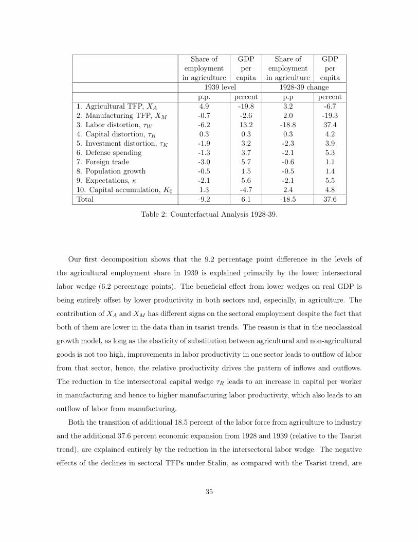
Share of GDP Share of GDPemployment per employment perin agriculture capita in agriculture capita

1939 level 1928-39 changep.p. percent p.p percent

1. Agricultural TFP, XA 4.9 -19.8 3.2 -6.72. Manufacturing TFP, XM -0.7 -2.6 2.0 -19.33. Labor distortion, τW -6.2 13.2 -18.8 37.44. Capital distortion, τR 0.3 0.3 0.3 4.25. Investment distortion, τK -1.9 3.2 -2.3 3.96. Defense spending -1.3 3.7 -2.1 5.37. Foreign trade -3.0 5.7 -0.6 1.18. Population growth -0.5 1.5 -0.5 1.49. Expectations, κ -2.1 5.6 -2.1 5.510. Capital accumulation, K0 1.3 -4.7 2.4 4.8Total -9.2 6.1 -18.5 37.6

Table 2: Counterfactual Analysis 1928-39.

Our first decomposition shows that the 9.2 percentage point difference in the levels of

the agricultural employment share in 1939 is explained primarily by the lower intersectoral

labor wedge (6.2 percentage points). The beneficial effect from lower wedges on real GDP is

being entirely offset by lower productivity in both sectors and, especially, in agriculture. The

contribution of XA and XM has different signs on the sectoral employment despite the fact that

both of them are lower in the data than in tsarist trends. The reason is that in the neoclassical

growth model, as long as the elasticity of substitution between agricultural and non-agricultural

goods is not too high, improvements in labor productivity in one sector leads to outflow of labor

from that sector, hence, the relative productivity drives the pattern of inflows and outflows.

The reduction in the intersectoral capital wedge τR leads to an increase in capital per worker

in manufacturing and hence to higher manufacturing labor productivity, which also leads to an

outflow of labor from manufacturing.

Both the transition of additional 18.5 percent of the labor force from agriculture to industry

and the additional 37.6 percent economic expansion from 1928 and 1939 (relative to the Tsarist

trend), are explained entirely by the reduction in the intersectoral labor wedge. The negative

effects of the declines in sectoral TFPs under Stalin, as compared with the Tsarist trend, are

35

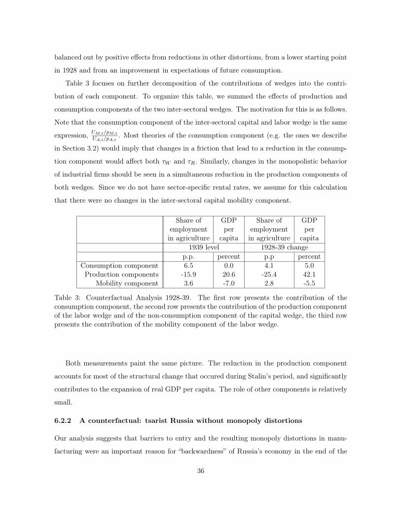
balanced out by positive effects from reductions in other distortions, from a lower starting point

in 1928 and from an improvement in expectations of future consumption.

Table 3 focuses on further decomposition of the contributions of wedges into the contri-

bution of each component. To organize this table, we summed the effects of production and

consumption components of the two inter-sectoral wedges. The motivation for this is as follows.

Note that the consumption component of the inter-sectoral capital and labor wedge is the same

expression, UM,t/pM,tUA,t/pA,t. Most theories of the consumption component (e.g. the ones we describe

in Section 3.2) would imply that changes in a friction that lead to a reduction in the consump-

tion component would affect both τW and τR. Similarly, changes in the monopolistic behavior

of industrial firms should be seen in a simultaneous reduction in the production components of

both wedges. Since we do not have sector-specific rental rates, we assume for this calculation

that there were no changes in the inter-sectoral capital mobility component.

Share of GDP Share of GDPemployment per employment perin agriculture capita in agriculture capita

1939 level 1928-39 changep.p. percent p.p percent

Consumption component 6.5 0.0 4.1 5.0Production components -15.9 20.6 -25.4 42.1

Mobility component 3.6 -7.0 2.8 -5.5

Table 3: Counterfactual Analysis 1928-39. The first row presents the contribution of theconsumption component, the second row presents the contribution of the production componentof the labor wedge and of the non-consumption component of the capital wedge, the third rowpresents the contribution of the mobility component of the labor wedge.

Both measurements paint the same picture. The reduction in the production component

accounts for most of the structural change that occured during Stalin’s period, and significantly

contributes to the expansion of real GDP per capita. The role of other components is relatively

small.

6.2.2 A counterfactual: tsarist Russia without monopoly distortions

Our analysis suggests that barriers to entry and the resulting monopoly distortions in manu-

facturing were an important reason for “backwardness” of Russia’s economy in the end of the

36

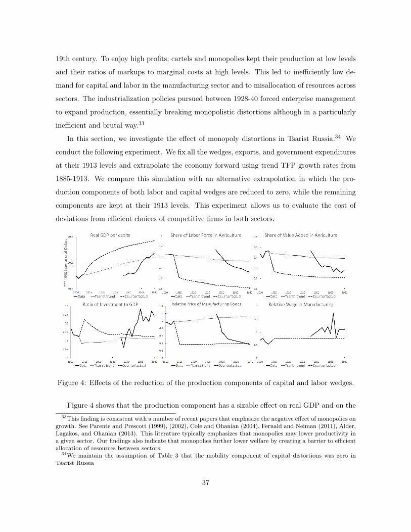
19th century. To enjoy high profits, cartels and monopolies kept their production at low levels

and their ratios of markups to marginal costs at high levels. This led to inefficiently low de-

mand for capital and labor in the manufacturing sector and to misallocation of resources across

sectors. The industrialization policies pursued between 1928-40 forced enterprise management

to expand production, essentially breaking monopolistic distortions although in a particularly

inefficient and brutal way.33

In this section, we investigate the effect of monopoly distortions in Tsarist Russia.34 We

conduct the following experiment. We fix all the wedges, exports, and government expenditures

at their 1913 levels and extrapolate the economy forward using trend TFP growth rates from

1885-1913. We compare this simulation with an alternative extrapolation in which the pro-

duction components of both labor and capital wedges are reduced to zero, while the remaining

components are kept at their 1913 levels. This experiment allows us to evaluate the cost of

deviations from efficient choices of competitive firms in both sectors.

Figure 4: Effects of the reduction of the production components of capital and labor wedges.

Figure 4 shows that the production component has a sizable effect on real GDP and on the33This finding is consistent with a number of recent papers that emphasize the negative effect of monopolies on

growth. See Parente and Prescott (1999), (2002), Cole and Ohanian (2004), Fernald and Neiman (2011), Alder,Lagakos, and Ohanian (2013). This literature typically emphasizes that monopolies may lower productivity ina given sector. Our findings also indicate that monopolies further lower welfare by creating a barrier to efficientallocation of resources between sectors.

34We maintain the assumption of Table 3 that the mobility component of capital distortions was zero inTsarist Russia

37

share of employment in agriculture. By 1940, real GDP in the absence of Tsarist monopoly dis-

tortions is 55 percent higher than in their presence. Since productivity growth is the same in the

two simulations by construction, all additional GDP growth is achieved through reallocation of

labor and accumulation of capital. Because the manufacturing sector is more capital-intensive,

the elimination of monopoly distortions generates an initial investment boom. It also leads

to a reallocation of additional 24 percentage points of employment from agriculture to manu-

facturing and a drop in the relative prices of manufacturing goods by about 65 percent. The

removal of monopoly distortions results in a large increase in consumption; relative to the ac-

tual Soviet data, this counterfactual achieves a much higher GDP per capita. The overall effect

is equivalent to a 47 percent permanent increase in aggregate consumption relative to Soviet

data.

The predictions of the neoclassical growth model for the behavior of labor allocation and

prices due to a removal of the production component of distortions are consistent with the

behavior of those variables in the Soviet data. In the actual data the production component of

distortions reduced almost to one by 1935 (Figure 3). The counterfactual drop in relative prices

and the reallocation of labor in the scenario without the production component of the labor

wedge are also remarkably consistent with the actual data in Soviet Russia (Figure 4). This is

also in line with the results in Table 2 which show that the production components account for

more than half of GDP growth and for virtually all labor reallocation. The behavior of prices in

the data is also consistent with the view of economic historians that prices played an important

allocative role in the Soviet economy and arose as an outcome of a decentralized bargaining

process between Soviet enterprises and government ministries rather than from being set in an

arbitrary fashion.35

Our analysis also contributes to the classical debate in development economics on whether

the rural-urban reallocation was first and foremost driven by the the development of modern35An early comprehensive study of Soviet prices by Harrison (1998) based on the archives of the former Soviet

planning commission and the statistical office argues that “The [planned] prices were quite distinct from theprices currently prevailing in the Soviet economy at any given time, wholesale and retail, regulated and free-market. These currently prevailing prices played important roles, even in a planned economy ...” Gregory andHarrison (2005) based on the recently revealed Stalin’s archives argue in favor of rational allocative price settingby Soviet firms: “Final allocations of products were achieved through contracting between ministries, ministrymain administrations, and enterprises. Decentralized contracting generated a degree of price flexibility, and thistells us much about the motivations, resources, and constraints of the agents involved ... The archives showthat price-setting was one of the most important activities of Soviet firms ...”.

38

industry in the cities or by the productivity growth in agriculture that pushes workers out

of that sector.36 Our results imply that these were the developments in the non-agricultural

sector that played a central role in the growth experience of Russia in 1885-1940. We find

that distortions in production, such as entry barriers and monopoly power, were the main

block to a more efficient allocation of resources between sectors in Tsarist Russia. Structural

transformation in 1928-40 was mainly achieved through the removal of such distortions. While

productivity in Soviet agriculture was at or below the Tsarist trend, the reduction in markups

and the increase in demand for labor seems to have played a critical role in Russia’s structural

transformation.37

7 Conclusion

In this paper, we use the neoclassical growth model to qualitatively and quantitatively study

the structural transformation of Russia in the late 19th and early 20th century. We extend the

wedge accounting methodology by paying special attention to prices in addition to quantities.

This allows us to decompose the wedges into their components and to differentiate between

various mechanisms. We find that the high level of the intersectoral labor wedge was the

main impediment to structural transformation of Tsarist Russia, and its reduction played by

far the most significant role during Soviet industrialization. In terms of the analysis of the

components of the labor wedge, we find that the key driver of the labor wedge was its production

component; this is consistent with the evidence on the importance of monopolies and entry

barriers in Tsarist Russia. The reduction in the production component of the wedge in Soviet

Russia explains essentially all of the observed structural transformation in 1928-40. Other

components of the labor wedge became more distorted. Thus, our findings cast doubt on the

most common explanation of slow transformation of Tsarist Russia – that archaic institutions

of land ownership precluded labor mobility across sectors. Our findings are also not consistent

with the “Big Push” theory. Furthermore, we find little evidence that the difference in TFP

growth across sectors is responsible for structural transformation.36See the seminal works by Lewis (1954) and Harris and Todaro (1970) on the role of the former and Nurkse

(1953), Schultz (1953), and Rostow (1960) on the role of the latter.37In our model, a large increase in agricultural productivity would also lead to structural change. However,

we do not observe such an increase in the Soviet data; agricultural productivity never caught up to the pre-1913trend.

39

We believe that our analysis of the most important barriers to the development of Tsarist

Russia and the factors behind Soviet industrialization is useful beyond the interests of economic

history. Our methodology of decomposing wedges into price components is applicable more

broadly to a variety of other settings. Our findings on the relative importance of components of

the labor wedge gives further support to the idea that frictions and prices play a significant role

in structural transformation (e.g., Caselli and Coleman, 2001). The fact that misallocation of

resources due to monopoly distortions plays a key role supports and further develops the findings

in the contexts of barriers to riches (Parente and Prescott, 2002), the U.S. Great Depression

(Cole and Ohanian, 2004), and the decline of the U.S. Rust Belt (Alder, Lagakos, and Ohanian,

2013). Our findings on the limited role of labor mobility restrictions and the absence of evidence

for the role of the “Big Push” is of broader interest to the economic development literature.

We now briefly note some other issues that we did not discuss in this paper. First, our

working paper version (Cheremukhin et. al., 2013) provides a much more complete description

of the historical accounts, more robustness exercises, and other counterfactuals. Second, we on

purpose avoided the discussion of welfare implications of various policies. Stalin’s era was one

of the most terrible episodes of Russian history with millions perishing in the famine of the

early 1930s and repressions in the late 1930s. Any welfare calculation must necessarily take a

stand on the costs of the lives lost. Thirdly, in this paper we did not discuss two periods of

Russian history that are of a particular interest to scholars of Russia. The period of the Civil

War and War Communism following the fall of Tsarist Russia is an example of a significant

economic disaster. We refer the reader to an impressive reconstruction of some of the economic

statistics during that period by Markevich and Harrison (2011a,b). The brief period of the

New Economic Policy in the 1920s saw a reintroduction of a limited market economy in Soviet

Russia that was cut short by Stalin. We refer an interested reader to a detailed analysis of the

New Economic Policy in the working paper version (Cheremukhin et. al., 2013).

40

References

Acemoglu, Daron (2008) Introduction to Modern Economic Growth, Princeton Univer-

sity Press.

Acemoglu, Daron, and Veronica Guerrieri (2008) “Capital Deepening and Nonbal-

anced Economic Growth,” Journal of Political Economy, 116(3), pp. 467-498.

Alder, Simeon, David Lagakos, and Lee Ohanian (2013) “The Decline of the U.S.

Rust Belt: A Macroeconomic Analysis,” mimeo, UCLA.

Allen, Robert C. (1997) “Agricultural Marketing and the Possibilities for Industrializa-

tion in the Soviet Union in the 1930s,” Explorations in Economic History, 34(4), pp. 387-410.

Allen, Robert C. (2003) Farm to Factory: a Reinterpretation of the Soviet Industrial

Revolution, Princeton University Press.

Anan’ich, Boris V. (1983) “The Economic Policy of the Tsarist Government and En-

terprise in Russia from the End of the Nineteenth through the Beginning of the Twentieth

Century.” in in Gregory Guroff and Fred V. Carstensen, eds., Entrepreneurship in Imperial

Russia and the Soviet Union. Princeton University Press.

Barsov, Alexander (1969) Balans Stoimostnykh Obmenov Mezhdu Gorodom i Derevnei.

Moscow: Nauka. [in Russian: The balance of the costs exchange between the city and the village]

Bergson, Abram, Roman Bernaut, and Lynn Turgeon (1955) “Basic Industrial

Prices in the USSR, 1928–1950: Twenty-Five Branch Series and Their Aggregation,” Santa

Monica: The Rand Corporation. Research Memorandum RM-1522.

Blackwell, William (1974) “Introduction” in Blackwell, William, ed. Russian Economic

Development: From Peter the Great to Stalin, NY: New Viewpoints.

Borodkin, Leonid, Brigitte Granville, and Carol Leonard (2008) “The Rural/urban

Wage Gap in the Industrialisation of Russia, 1884–1910,” European Review of Economic His-

tory, 12, pp. 67–95.

Buera, Francisco and Joe Kaboski (2009) “Can Traditional Theories of Structural

Change Fit the Data?” Journal of the European Economic Association, 7(2-3), pp. 469-477.

Buera, Francisco and Joe Kaboski (2012a) “Scale and the Origins of Structural

Change,” Journal of Economic Theory, 147(2), pp. 684-712.

41

Buera, Francisco and Joe Kaboski (2012b) “The Rise of the Service Economy,” Amer-

ican Economic Review, 102(6), pp. 2540-69.

Caselli, Francesco (2005) “Accounting for Cross-Country Income Differences,” Handbook

of Economic Growth (Aghion and Durlauf, eds.), North-Holland.

Caselli, Francesco, and Wilbur John II Coleman (2001) “The U.S. Structural

Transformation and Regional Convergence: A Reinterpretation,” Journal of Political Econ-

omy, 109(3), pp. 584-616.

Paul Castaneda Dower, and Andrei Markevich (2013) “Land Tenure and Produc-

tivity in Agriculture: The Case of the Stolypin Reform in Late Imperial Russia.” Mimeo, New

Economic School.

Central Statistical Committee of the Interior Ministry (1907) Statistika Zem-

levladenia 1905 g. Saint Petersburg. [In Russian: Land Ownership Statistics in 1905]

Chandler, Alfred D., Jr. (1977) The Visible Hand: The Managerial Revolution in

American Business. The Belknap Press of Harvard University Press.

Chari, V. V., Patrick Kehoe, and Ellen McGrattan (2007) “Business Cycle Ac-

counting,” Econometrica, 75(3), pp. 781-836.

Cheremukhin, Anton, Mikhail Golosov, Sergei Guriev, and Aleh Tsyvinski

(2013) “Was Stalin Necessary for Russia’s Economic Development?” NBER Working Paper

19425.

Cole, Harold, and Lee Ohanian (2002) “The U.S. and U.K. Great Depressions Through

the Lens of Neoclassical Growth Theory,” American Economic Review, 92(2), pp. 28-32.

Cole, Harold, and Lee Ohanian (2004) “New Deal Policies and the Persistence of the

Great Depression: A General Equilibrium Analysis,” Journal of Political Economy, 112(4), pp.

779-816.

Crisp, Olga (1978) “Labor and Industrialization in Russia,” Cambridge Economic History

of Europe, Vol. 7, part 2. Cambridge University Press.

Davies, Robert (1990) From Tsarism to the New Economic Policy. Macmillan Academic

and Professional Ltd.

Davies, R.W., Mark Harrison and S.G. Wheatcroft (1994) The Economic Trans-

formation of the Soviet Union, 1913-1945 ; New York : Cambridge University Press.

Davies, R.W., and S.G. Wheatcroft (2004) The Years of Hunger: Soviet Agriculture,

42

1931-1933, Palgrave Macmillan.

Falkus, M.E. (1972) The Industrialization of Russia 1700-1914. Macmillan.

Fernald, John, and Brent Neiman (2011) “Growth Accounting with Misallocation:

Or, Doing Less with More in Singapore,” American Economic Journal: Macroeconomics, 3(2),

pp. 29-74.

Gerschenkron, Alexander (1951) “A Dollar Index of Soviet Machinery Output, 1927-

1928 to 1937.” RAND Corporation, Report R-197.

Gerschenkron, Alexander (1965) “Agrarian Policies and Industrialization, Russia 1861–

1917,” In: Habakkuk, H.J., Postan, M. (Eds.), The Cambridge Economic History of Europe.

Volume VI: The Industrial Revolutions and After: Incomes, Population and Technological

Changes (II). Cambridge University Press, Cambridge, England, pp. 706-800.

Gollin, Douglas, David Lagakos, and Michael E. Waugh (2014) “The Agricultural

Productivity Gap,” Quarterly Journal of Economics, 129 (2): 939-993.

Gollin, Douglas, Stephen Parente, and Richard Rogerson (2002) “The Role of

Agriculture in Development," American Economic Review, 92(2), pp. 160-164.

Goodwin, Barry, and Thomas Grennes (1998) “Tsarist Russia and the World Wheat

Market,” Explorations in Economic History, 35, pp. 405–430.

Gregg, Amanda G. (2015) “Factory Productivity and the Concession System of Incor-

poration in Late Imperial Russia, 1894-1908.” Mimeo, Middlebury College.

Gregory, Paul (1972) “Economic Growth and Structural Change in Tsarist Russia: A

Case of Modern Economic Growth?” Soviet Studies, 23(3), pp. 418-434.

Gregory, Paul (1982) Russian National Income, 1885-1913, Cambridge University Press.

Gregory, Paul (1994) Before Command: The Russian Economy From Emancipation to

Stalin, Princeton: Princeton University Press.

Gregory, Paul, and Mark Harrison (2005) “Allocation under Dictatorship: Research

in Stalin’s Archives,” Journal of Economic Literature, 43(3), pp. 721-761.

Gregory, Paul, and Robert Stuart (1986) Soviet Economic Structure and Performance.

New York: Harper & Row.

Guinnane, Timothy, Ron Harris, Naomi Lamoreaux, and Jean-Laurent Rosen-

thal (2007) “Putting the Corporation in its Place.” Enterprise and Society 8(3): pp. 687 -

729.

43

Harris, John R., and Michael P. Todaro (1970) "Migration, Unemployment and De-

velopment: A Two-Sector Analysis,” American Economic Review, 60(1), pp.126-42.

Harrison, Mark (1998) “Prices, Planners, and Producers: An Agency Problem in Soviet

Industry, 1928-1950,” Journal of Economic History 58(4), pp. 1032-1062.

Hayashi, Fumio, and Edward Prescott (2008) “The Depressing Effect of Agricultural

Institutions on the Prewar Japanese Economy,” Journal of Political Economy, 116(4), pp. 573-

632.

Herrendorf, Berthold, Richard Rogerson, and Akos Valentinyi (2013). “Two Per-

spectives on Preferences and Structural Transformation,” American Economic Review, 103(7),

pp. 2752-89.

Hunter, Holland (1988) “Soviet Agriculture with and without Collectivization, 1928-

1940,” Slavic Review, 47(2), pp. 203-216.

Hunter, Holland and Janusz M. Szyrmer (1992) Faulty Foundations: Soviet Eco-

nomic Policies, 1928-1940. Princeton University Press.

Kitanina, T.M. (1995) “Torgovlya.” in Anfimov A.N. and Korelin A.P., eds., Rossiya

1913. Institute of Russian History of the Russian Academy of Science, Saint Petersburg. [In

Russian: “Trade” in “Russia 1913”]

Kongsamut, Piyabha, Sergio Rebelo, and Danyang Xie (2001) “Beyond Balanced

Growth,” Review of Economic Studies, 68(4), pp. 869-82.

Lagakos, David, and Michael E. Waugh (2013) "Selection, Agriculture, and Cross-

Country Productivity Differences." American Economic Review, 103(2), pp. 948-80.

von Laue, Theodore (1974) “The State and the Economy.” in Blackwell, William, ed.

Russian Economic Development: From Peter the Great to Stalin, NY: New Viewpoints.

Lenin, Vladimir (1972) Lenin. Collected works. Vol 2. Progress Publishers, Moscow.

Lewis, W. Arthur (1954) “Economic Development with Unlimited Supplies of Labor,”

Manchester School 22, pp. 139-192.

Markevich, Andrei, and Mark Harrison (2011a) “Great War, Civil War, and Re-

covery: Russia’s National Income, 1913 to 1928,” Journal of Economic History, 71(3), pp.

672-703.

Markevich, Andrei, and Mark Harrison (2011b) “Russia’s National Income: Ap-

pendix” Online appendix.

44

Mau, Vladimir, and Tatiana Drobyshevskaya (2013) “Modernization and the Russian

Economy: Three Hundred Years of Catching Up,” in Michael Alexeev and Shlomo Weber, eds.,

The Oxford Handbook of the Russian Economy, Oxford University Press, pp. 29-51.

Meng, Xing, Nancy Qian, and Pierre Yared (2014) “The Institutional Causes of

Famine in China, 1959-61,” mimeo, Yale University.

Metzer, Jacob (1973) “Some Economic Aspects of Railroad Development in Tsarist Rus-

sia,” Journal of Economic History 33(1), pp. 314-316.

Metzer, Jacob (1974) “Railroad Development and Market Integration: The Case of

Tsarist Russia,” Journal of Economic History 34(3), pp. 529-550.

Metzer, Jacob (1976) “Railroads in Tsarist Russia: Direct Gains and Implications,”

Explorations in Economic History 13, pp. 85-111.

Moorsteen, Richard H., and Raymond P. Powell (1966) The Soviet Capital Stock,

1928-1962, Homewood, Ill., R. D. Irwin.

Mulligan, Casey (2002) “A Century of Labor–Leisure Distortions,” Working Paper 8774,

National Bureau of Economic Research.

Murphy, Kevin M., Andrei Shleifer and Robert W. Vishny (1989) “Industrializa-

tion and the Big Push.” Journal of Political Economy, 97(5), pp. 1003-1026.

Nafziger, Steven (2010) “Peasant Communes and Factor Markets in late Nineteenth-

century Russia,” Explorations in Economic History, 47(4), pp. 381–402.

Ngai, L. Rachel, and Christopher Pissarides (2007) “Structural Change in a Multi-

sector Model of Growth,” American Economic Review, 97(1), pp. 429-443.

Nurkse, Ragnar (1953) Problems of Capital Formation in Underdeveloped Countries.

Oxford: Oxford University Press.

Owen, Thomas (1991) The Corporation under Russian Law, 1800-1917, Cambridge Uni-

versity Press.

Parente, Stephen, and Edward Prescott (1999) “Monopoly Rights: A Barrier to

Riches,” American Economic Review, 89(5), pp. 1216-1233.

Parente, Stephen, and Edward Prescott (2002): Barriers to Riches, MIT Press.

Pipes, Richard (1997) Russia under the Old Regime. Penguin Books.

Restuccia, Diego, Dennis Tao Yang, and Xiaodong Zhu (2008) “Agriculture and

Aggregate Productivity: A Quantitative Cross-country Analysis,” Journal of Monetary Eco-

45

nomics, 55(2), pp. 234-250.

Rostow, Walt Whitman (1960) The Stages of Economic Growth, London: Cambridge

University Press.

Schultz, Theodore W. (1953) The Economic Organization of Agriculture. New York:

McGraw-Hill.

Shepelev, Leonid E. (1973) Aktsionernye Kompanii v Rossii. Leningrad: Nauka. [In

Russian: Joint Stock Companies in Russia.]

Spulber, Nicolas (2003) Russia’s Economic Transitions: From Late Tsarism to the New

Millennium, Cambridge University Press.

Strumilin, Stanislav (1960) Ocherki Ekonomicheskoi Istrorii Rossii. Moscow: izda-

tel’stvo sotsial’no-ekonomicheskoi literatury. [In Russian: Essays in Russian Economic History.]

Strumilin, Stanislav (1982) Problemy Ekonomiki Truda. Moscow: Nauka. [In Russian:

The problems of Labor Economics.]

Stokey, Nancy (2001) “A Quantitative Model of the British Industrial Revolution, 1780-

1850,” Carnegie-Rochester Conference Series on Public Policy, 55, pp. 55-109.

Tugan-Baranovsky, Mikhail (1898, republished in 1997) Russkaya Fabrika v Proshlom

i Nastoyaschem. Moscow: Nauka [In Russian: Russian Factory in the Past and Today.]

46

Appendix A: Construction of data

A.1 Capital stock

A.1.1 Russia 1885-1913

For Russia in 1885-1913 all data are from Gregory (1982) using 1913 prices. Capital in agricul-

ture is a sum of value of livestock (Table H.1), accumulated agricultural equipment (Table I.1)

and net fixed capital stock in agriculture (Table J.1). Agricultural structures include rural resi-

dential structures, and Gregory does not provide a separate estimate of those. Gregory provides

estimates of livestock, and net capital stock but gives investment in agricultural equipment. We

derive the stock of agricultural equipment with the perpetual inventory method by assuming

a depreciation rate of 5 percent per year. Capital stock in non-agriculture is defined as the

value of accumulated industrial equipment (Table I.1), net stock of industrial structures (Table

J.1), industry inventories (table K.1), and railroads (Table L.1). The values for the stock of

structures, inventory, railroads, and urban housing are taken directly from Gregory while the

stock of accumulated industrial equipment is obtained by perpetual inventory method assuming

5 percent depreciation.

This definition of capital stock includes rural residential housing in agricultural capital stock

but does not include urban residential housing in any measure of capital stock. The reason for

this is as follows. Ideally, we would like to exclude housing stock from all measures of capital.

Gregory does not provide a breakdown of rural capital between residential and nonresiden-

tial. We do not include urban residential housing into non-agricultural capital stock since the

estimates of urban capital stock differ dramatically for pre-1913 and post-1928 Russia which

we view as unrealistic. Total capital stock is defined as a sum of capital stock in agriculture

and non-agriculture. We computed investments in each sector from the series of capital stocks

assuming 5 percent depreciation.

A.1.2 Russia 1928-1940

For Russia in 1928-1940 we use data from Moorsteen and Powell (1966). All data are in 1937

prices. We use the data on the composition of gross residential fixed capital stock (Table 3-3)

to find the fraction of urban residential capital stock in gross residential fixed capital stock.

We assumed that the same ratio holds for net residential capital stock (Table T-15) to find

47

the value of net urban residential capital stock. We define non-agricultural capital stock as net

nonresidential, nonagricultural capital stock (table T-25). This definition includes industrial

fixed structures, equipment and inventories. We define agricultural capital stock as net fixed

capital stock minus net nonresidential nonagricultural capital stock and minus the value of

urban residential housing. Total capital stock is defined as a sum of capital stock in agriculture

and non-agriculture.

A.2 Exports and imports

The data for the total volume of exports and imports for Tsarist Russia are from Gregory

(1982), Table M-1. We use the data from Davies (1990, Table 56) to find the composition of

exports and imports for 1913. We assume that the same composition holds for 1885-191338 and

compute net exports of agricultural goods and net imports of non-agriculture goods. The data

for the volume of exports and imports for the USSR from 1928 to 1938 are from Davies et al.

(1994). They provide an index of exports and imports relative to 1913, and we use the numbers

for 1913 trade from Gregory (1982) to obtain the volume of trade in 1913 prices. We impute

the values for 1939 and 1940 by assuming that they remain at the 1938 level. We use the data

from Davies (1990, Table 58) to find composition of exports and imports for 1927/1928. We

assume that the same composition holds for 1928-1940 and compute net exports of agricultural

goods and net imports of non-agricultural goods.

A.3 Output, consumption and investment by sector

A.3.1 Russia 1885-1913

We computed investments in each sector from the series of capital stocks assuming 5 percent

depreciation. We computed GNP from NNP series in Gregory (1982), Table 3.1, by adding 5

percent depreciation to the total capital stock. We did not find reliable data for value added

in manufacturing and agriculture for all years. Gregory (1982) in Table 3.6 reports that 50.7

percent of value added was produced in agriculture in 1913. He also provides numbers for

retained consumption of agricultural goods which were not marketed by the peasants (Table

M.1) for all time periods. We assume that the fraction of value added of agricultural production38Kitanina (1995) shows that the composition of trade changed very slowly in 1899-1913 (there are no reliable

data before 1899). The share of industrial products in exports was 4.7% in 1899-1903 and 5.6% in 1913; theshare of industrial products in imports was 29.3% in 1899-1903 and 32.8% in 1913.

48

to the retained consumption is at the same level as in 1913 to obtain the estimate of value

added in agriculture during 1885-1913. The value added in manufacturing is obtained by

subtracting the value added in agriculture from GNP. Gregory reports breakdown of imperial

and local government expenditures for selected years (Tables F.4 and G.4). For the benchmark

analysis we took defense expenditures as our measure of government sector and we checked the

robustness of our conclusion by added administrative expenditures. The data for the missing

years was obtained by linear interpolation. To obtain relative prices, we computed nominal

value added of agriculture following the same steps as we did for the value added in agriculture

in 1913 prices. The ratio of the two gives us a price deflator for agriculture. Gregory in Tables

3.1 and 3.2 reports net investments in current prices and 1913 prices, which allow us to compute

the investment price deflator and depreciation in current prices. Using Gregory’s estimates of

national income in current prices and our estimates of depreciation in current prices we obtain

GNP in current prices. By subtracting the value of agriculture in current prices we obtain the

value of manufacturing in current prices and the price deflator for manufacturing goods. The

ratio of the price deflator for agricultural goods to the price deflator of manufacturing goods

yields the relative price of agricultural goods.

Data for military spending also come from Gregory (1982), Tables F.4 and G.4.

A.3.2 Russia 1928-1940

Moorsteen and Powell (1966, Table P.1) provide estimates of GNP and production by sector

in 1937 prices. We measure the agricultural sector as total output in agriculture, and the

manufacturing sector as GNP minus the agricultural sector. Finding appropriate series for

relative prices is particularly challenging. We rely on the work of Allen (1997, Table A2) who

calculates the ratio of wholesale industrial prices to wholesale agricultural prices based on the

previous work of Bergson et al. (1955) and Barsov (1969).

We have data series for real GDP growth in 1913 rubles for Russia. We also have real

GDP in 1990 international dollars for 1913. To construct real GDP per capita, we use real

GDP per capita in international dollars for 1913, and then apply real GDP growth rates (in

constant rubles and dollars) to construct real GDP in international dollars for other years in

the 1885-1913 period. This series may differ slightly from real GDP in international dollars for

other years, as the relative prices might have changed. However, our index captures well the

49

general patterns. The fraction of agricultural value added measures the ratio of agricultural

value added in 1913 prices to real GDP in 1913 prices.

Data for military spending are from Moorsteen and Powell (1966), Table P-1.

A.4 Population, labor force and wages

A.4.1 Russia 1885-1913

The data for population is from Gregory (1982), Table 3.1. He reports the data for the territory

of Russian empire excluding Finland and we follow his convention. We obtain the composition

of the labor force from Davies (1990) and Gregory’s estimates. Davies (1990), Table 3, provides

an estimate of the composition of the labor force by sector in 1913. Gregory (1982), Table 6.3,

reports growth rates for labor force by sector for different time periods during 1885-1913. We

use these growth rates to backtrack labor force for years before 1913.

Calculating sectoral employment or even the labor force is difficult both for the Tsarist and

for Soviet periods. Unlike data on economic aggregates, there are little reliable data on sectoral

employment before 1913. Tsarist Russia conducted only one national census, in 1897. There

are employment records from the administrative data in some heavy industries, but for the

rest of the economy there are only sporadic surveys. For this reason, Gregory (1982) does not

provide annual employment numbers but only the estimates of growth rates of labor force for

agriculture, manufacturing, and services for 1883-87 to 1897-1901 and for 1883-1897 to 1909-

1913. An early Soviet economic historian Gukhman used census and archival data to estimate

composition of the labor force in 1913 which was then reproduced in Davies (1990). As in

the census as well as Gukhman and Davies, we define sectoral employment for each worker

according to the self-reported primary occupation. This definition seems to be the only way

to obtain a consistent definition of the sectoral labor force for Tsarist Russia and the Soviet

Union. It almost certainly overestimates the true employment in agriculture and underestimates

employment in manufacturing. There is substantial evidence that agricultural workers spent a

part of their time in non-agricultural activities, such as seasonal manufacturing work in the city

and self-employment (promysly). We also need to take a stand on how to treat employment

of women. The available employment records before 1913 are from select heavy industries

that predominantly employed men. As the non-agricultural sector expanded dramatically after

1928, so did the fraction of women in non-agricultural employment. Based on this evidence one

50

may be tempted to conclude that female labor force participation significantly increased. At

the same time, there is evidence that before 1913 female labor force participation in agriculture

was very high, as women had to replace men who were employed as migrant workers in urban

industries. For example, Crisp (1978) in her study of pre-WWI Russian labor markets points

out that although in factory industries there were only 800,000 women compared with several

million men, in peasant farms “the proportion of women undoubtedly exceeded that of male,

especially if all-year-around averages are taken into account”. Since there are no reliable figures

regarding female labor force participation, we do not treat women and men differently and

assume that all of the working age population is a part of the labor force.

Our data on wages for 1885-1913 come from Allen (2003) and Strumilin (1982). The agri-

cultural wages come from the data on male daily wage (Strumilin, 1982, Table 2B, p. 253)

which we then multiply by 205 days per year to obtain the annual wage; according to Table

21, p. 268, agricultural workers worked for 104.2 days in the summer and 100.8 in the winter

season. The non-agricultural wages for 1900-1913 are provided in Strumilin (1982, p. 293).

Then we use the data on wages of day laborers and factory workers (Allen, 2003, Figure 2.2)

to calculate the changes in wages in 1885-1900; taking the 1900 level from Strumilin (1982, p.

293) we then calculate the wages in 1885-1899. The data on wages for unskilled construction

workers in St Petersburg are from Strumilin (1960, Table 13, p. 113).

A.4.2 Russia 1928-1940

We use population numbers from Davies et al. (1994), Table 1. In order to obtain the data on

the composition of the labor force, we use both census data (from the 1926 and 1939 censuses)

and the official estimates provided in selected interim years (Davies et al., 1994, Tables 11 and

12, respectively). The latter do not cover all of the non-agricultural labor force but give a

reasonably good approximation of the growth rate of the non-agricultural labor force over the

entire time period. According to the census data, the non-agricultural labor force increased by

a factor 3.37 between 1926 and 1939, while official survey numbers show an increase of 3.19

between 1928 and 1940 (Davies et al. 1994, p. 280 state that the number for 1940 partially

includes the workers in the new territories excluding certain categories of non-agricultural

employees).

From 1926 census (Davies et al., 1994, Table 11) we obtain the composition of employment

51

by sector. Davies et al.’s data come from Gukhman (1926) who also provides data on the

employment composition in 1913 using the same methodology. This allows us to reconcile the

data on employment structure in 1913 and 1926. We assume that each sector covered by the

survey data grows at the same rate as implied by the surveys. This gives us an estimate of non-

agricultural employment for each year. The implied increase in the non-agricultural employment

is 3.36, which closely matches the implied growth of non-agricultural employment from 1939

census. To find agricultural employment we use total employment and non-agricultural em-

ployment and find agricultural employment as residual. The ratio of employment to population

comes from censuses: it was 49 percent in 1926 and 50 percent in 1939 In order to obtain the

total labor force in the intermediate years and in 1940, we use a linear interpolation based on

1926 and 1939 data points.

Our data on farm and non-farm wages (consumption) in 1928, 1932-39 come from Allen

(2003, Table 7.5). We use linear interpolation of the ratio of agricultural to non-agricultural

wages for the missing years 1929-31. For the year 1940 we take the ratio of agricultural to

non-agricultural wages from 1939.

A.5 Adjustment for border changes, conversion prices

Using the procedure above we obtained two data sets, one for Russia in 1885-1913 in 1913

borders (excluding Finland) and in 1913 prices and the other one for the USSR in 1928-1940

in pre-1940 borders and in 1937 prices. In this Section we discuss the conversion of all prices

and quantities to comparable units. The territory of Russian empire excluding Finland is

21,474 sq km, while the territory of the USSR in pre-1940 borders is 21,242 sq km (Markevich

and Harrison, 2011a, Table 2). Thus the areas of the two territories are quite similar, and

therefore we assume that land endowments are the same in the two periods and do not make any

border adjustments.39 Markevich and Harrison (2011b) report (Table A10) that the fraction

of agriculture in NNP in Russian Empire excluding Finland was 44.3 percent in 1913 (50.9

percent if forestry, fishing and hunting is included in definition of agriculture) and in USSR

interwar borders was 44.4 percent (50.8 percent with forestry, fishing and hunting).39While land endowment remained the same, Russian empire lost richer territories (Finland, Poland, Western

Belarus and Ukraine, Caucasus) and gained poorer territories in Central Asia. Tsarist NNP in 1913 measuredin the USSR interwar borders would decrease from 22 mln rbl to 16.5 mln rbl (Markevich and Harrison, 2011a,Table 1). In the context of our model these differences are reflected in TFPs, and therefore we do not recomputeTsarist output in Soviet borders.

52

Markevich and Harrison (2011a) also report that NNP in 1913 prices in Russia increased

by 9.6% between 1913 and 1928. In per capita terms this amounts to a 3.6% fall. Given

that the sectoral composition of GDP did not change we use this growth rate to calculate the

sectoral value added in agriculture and manufacturing in year 1928 in 1913 prices adjusting for

population changes. Once we have Y A1928 in both 1937 prices (from Moorsteen and Powell) and

in 1913 prices (from Gregory and from Markevich and Harrison) we can calculate the ratio of

1937 and 1913 prices in the agricultural sector; we arrive at the factor of 6.65. We carry out

a similar calculation for the non-agricultural sector and find that non-agricultural prices grew

by the factor of 6.38 between 1913 and 1937.

Appendix B: A model of the “Big Push”

In this Section we show how to incorporate a version of the “Big Push” model of Murphy, Shleifer

and Vishny (1989) into a two-sector growth model and derive its predictions for structural

change and components of our wedge decomposition.

As in Murphy, Shleifer and Vishny (1989) we assume that manufacturing consists of a

continuum of goods i ∈ [0, 1]. Each manufacturing good can be produced using either “tra-

ditional” or “modern” technology. The traditional technology has constant returns to scale

with productivity normalized to one. The modern technology in sector i requires initial fixed

cost investment of D units of labor; the firm that has made this investment then becomes a

monopolist in that sector and operates a constant returns to scale technology with productiv-

ity X > 1. In addition, there is an agricultural good which can only be produced through a

constant returns to scale technology with productivity 1.

Consumers maximize the utility of consumption minus disutility of labor

max

η ln cA + (1− η)

ˆ 1

0

ln c (i) di−∆1 [modern]

(15)

subject to the budget constraint

pAcA +

ˆ 1

0p (i) c (i) di = Y.

Here cA is the consumption of the agricultural good, pA is the price of the agricultural good,

c (i) is the consumption of manufacturing good i, p(i) is the price of the manufacturing good i,

53

η is the parameter of the utility function (the relative weight of the agricultural consumption),

Y is the consumer’s income (consisting of profits and wages), and ∆1 [modern] is his disutility

of labor which is zero if the consumer works in the traditional sector and is ∆ > 0 if he works

in the modern sector. Like in Murphy, Shleifer and Vishny (1989), each worker inelastically

supplies one unit of labor, and the disutility of working in the modern sector results in a wage

premium in the modern sector.

The total labor force is normalized to 1, NA is the labor employed in agriculture, NM =´ 10 N (i) di is the total employment in manufacturing (where N(i) is the employment in sector

i). We shall denote wA the wage in agricultural sector and wM and w′M the wages in the

traditional and the modern manufacturing sectors, respectively.

Now we can solve the model. Consumer demand is

cA =Y

pAη,

c (i) =Y

p (i)(1− η) . (16)

Since agricultural sector has only constant returns to scale technology, prices and wages are

always equal to 1: pA = wA = 1.

Let us now solve for the incentives to industrialize. If sector i uses the traditional technology,

the prices and wages are also equal to 1: pM = wM = 1. The producers make zero profits. If a

sector moves to the modern technology, it sets the prices using its monopoly power and taking

into account the demand function (16). Competition from the traditional sector implies that

the profit maximizing price for a monopolist is 1.

If a sector i industrializes, it receives a profit yi−w′M( yiX +D

), where yi = Y (1− η) is the

demand for its good (16) at price p(i) = 1. Therefore, the manufacturing sector has incentives

to industrialize if and only if

yi = Y (1− η) > Dw′M

1− w′M/X.

As all manufacturing sectors are symmetric, there can only be two stable equilibria. In one

equilibrium (‘no-industrialization’), all manufacturing sectors use traditional technology. In the

other, ‘industrialization’, equilibrium, all manufacturing goods are produced through modern

technology. In each case, every manufacturing sector produces the same amount c(i) = cM =´ 10 c (i) di = Y (1− η).

54

When manufacturing does not industrialize, the equilibrium is analogous to our baseline

frictionless economy in Section 3.2. In particular, from the optimality conditions

1− ηη

cAcM

pApM

= 1,

and the fact that pM = pA = 1 and feasibility constraints we get

1− ηη

NA

NM= 1,

NA +NM = 1.

Therefore

NA = η; NM = 1− η.

The consumer’s income is Y = 1. This equilibrium exists if and only if

1− η < Dw′M

1− w′M/X. (17)

Let us now consider the equilibrium where all manufacturing firms industrialize. We will

use c′j , p′j , w

′j , N

′j (j = A,M) to denote the parameters of this equilibrium. We still have

p′M = p′A = 1, but now

1− ηη

N ′AXN ′M

= 1,

N ′A +N ′M +D = 1.

This immediately implies

N ′A =(1−D) ηX

1− η + ηX, N ′M =

(1−D) (1− η)

1− η + ηX.

The consumer’s income is

Y ′ = pAc′A + pMc

′M = XN ′M +N ′A =

(1−D)X

1− η + ηX.

The wages in manufacturing are determined by ln (Y ′ − (w′M − 1)) = ln (Y ′)−∆ which implies

w′M = 1 +(1−D)X

1− η + ηX

(1− e−∆

).

The industrialization equilibrium exists whenever

Y ′(1− η) > Dw′M

1− w′M/X. (18)

55

If the fixed cost of industrialization D is sufficiently low and the productivity in the modern

sector X is sufficiently high then Π′ = (1−D)X1−η+ηX > Π = 1 so that for some range of ∆ both (17)

and (18) hold. In this case there is a multiplicity of equilibria (and therefore a rationale for the

“Big Push”).

Let us now compare the two equilibria. In the industrialization equilibrium, TFP in man-

ufacturing is higher:XN ′MN ′M +D

> w′M > 1.

The labor wedge isX > 1 in the industrialization equilibrium and 1 in the no-industrialization

equilibrium. The production component is higher in the industrialization equilibrium:

X

w′M>N ′M +D

N ′M> 1.

The mobility component is also higher:

w′Mw′A

= w′M > 1 =wMwA

.

The ratio of prices and the ratio of marginal utilities are the same in both equilibria; hence

the consumption component of the labor wedge is the same.

Whenever both equilibria exist, the labor force in agriculture is higher in the industrializa-

tion equilibrium:

N ′A =(1−D) ηX

1− η + ηX> NA = η.

The intuition for this result is straightforward. The industrialization equilibrium exists if and

only if industrialization results in higher aggregate income Y ′ > Y . This in turn implies that

industrialization results in a higher demand for agricultural products. As the technology in

agriculture does not change, increase in agricultural production requires an increase in agri-

cultural employment. The labor moves to agriculture from manufacturing (where higher TFP

allows to produce more output with less labor).

56