the hierarchical real-time control of high speed trains for automatic · pdf...

The hierarchical real-time control of high speed trains for automatic train operation

Q. Y. Wang, P. Wu, Z. C. Liang & X. Y. Feng Southwest Jiaotong University, China

Abstract

The on-board controllers of high speed trains have been used to relieve drivers’ work by introducing a cruising control strategy or a target-speed automatic control strategy. However, the two control strategies above can only play a minor role during train operation, and the punctuality should be ensured by the train driver and the gradient profile may not be utilized to reduce energy consumption without debasing the punctuality. This paper investigates the real-time control problem of high speed trains, and then proposes a hierarchical control strategy to reduce energy consumption and improve the punctuality of the train operation planned by the railway timetable. The control strategy comprises of two modules, one of which is a speed profile planner, and the other is a speed tracking actuator. In the speed profile planner, an efficient algorithm via solving the optimal switching of adjoint variable based on the maximum principle is adopted to calculate the optimal speed profile of the train running section, meeting both the objective of energy consumption minimization and punctuality constraint. Then an active disturbance rejection controller is designed as the actuator to track the planned speed profile, implementing an accurate tracking of the accelerating process, cruising process and decelerating process. An extended state observer is designed to produce real-time estimates and compensation for the total disturbance. Simulations show that the hierarchical controller can ameliorate train operation effectively, from the aspects of planning and self-regulating ability which can improve operation punctuality offered by the speed profile planner, energy saving and riding comfort mainly offered

by the speed tracking actuator with proper parameter values. Keywords: automatic train operation (ATO), energy-efficient control, train control, active disturbance rejection control (ADRC).

Computers in Railways XIV 17

www.witpress.com, ISSN 1743-3509 (on-line) WIT Transactions on The Built Environment, Vol 135, © 2014 WIT Press

doi:10.2495/CR140021

1 Introduction

With the rapid development of rail passenger traffic, more and more attention has been paid to the quality of transportation service of high speed railway, which requires the high speed trains not only to meet the basic safety requirements, but also to ensure punctuality during the whole journey. Therefore, drivers or on-board equipment named ATO (Automatic Train Operation), are required to improve economic efficiency by reducing traction energy consumption, taking full advantage of the slack journey time planned by the railway timetable, compared with the flat-out operation time of trains, and potential of the line ramps as well. Nowadays, the on-board controllers of high speed trains for automatic speed regulating have been used to relieve drivers’ work by importing a cruising control strategy or a target-speed automatic control strategy. With the help of the cruising control strategy, drivers can press the cruising operation button on the driver table to make the train run at desired holding speed and switch to the manual mode when the train must undergo an accelerating or decelerating process. And with the help of the target-speed automatic control strategy, drivers just need to decide the target speed and when the train should enter the target-speed control mode and when to leave. However, the two control strategies above can just play a minor role during train operation, and the punctuality should be ensured by train drivers and the gradient profile may not be utilized to reduce energy consumption without debasing the punctuality. This paper will introduce a new hierarchical control strategy to reduce energy consumption and improve the punctuality of the train operation planned by railway timetable. The control strategy comprises of two modules, one of which is a speed profile planner, and the other is a speed tracking actuator. The speed profile planner will search optimal speed profile which meets both the objective of energy consumption minimization and punctuality constraint. Studies undertaken by many researchers in [1–6] have found that optimal train regime sequence includes full power, partial power, cruise control, coasting and full braking. In [4], the calculus of the adjoint variable and state variable is used to prove the existence and uniqueness of optimal regimes when there are no steep gradients in intervals or only one steep gradient between two speed holding intervals without considering the influence of speed limitation. In [6], the switching principles of optimal regimes are deduced by using maximum principle for trains that can feed energy back to traction net when braking regime is applied. However, the discussion about the influence of speed limitation is quite rough. In [7], by introducing driving experience from excellent drivers, a heuristic algorithm is proposed to search for switching points of regimes. But the optimality of this method is not validated. The optimal searching algorithm proposed in this paper will discuss the local optimal linkage of the train between two adjacent speed holding intervals in detail, which is the basic element of the optimal linkage of the train within a whole operation section according to the partitions of speed holding intervals described in Section 2.3. The speed profile planner will offer an integrated optimal speed profile as the reference

18 Computers in Railways XIV


speed commands to the actuator of high speed train, including a series of speed holding process in partial power mode or partial braking mode, and transition process which may be accelerating or decelerating process in full power, coasting or full braking mode. The active disturbance rejection controller (ADRC) is proposed by Han [8] in 1998, which has been adopted in plenty of applications for system control in [9–11]. As the actuator of high speed train, the ADRC is designed to track the planned speed profile, implementing an accurate tracking of the accelerating process, cruising process and decelerating process. And an extended state observer (ESO) is designed to produce real-time estimates and compensation for the total disturbance in the ADRC. Besides the transition process part of the ADRC is adopted to arrange train’s accelerating and decelerating tracking according to system ability of the train and passengers’ comfort.

2 Optimal speed profile planner

2.1 Mathematical model of train operation

In order to simplify the description of energy-efficient of train control problem, basic assumptions are put forward as follows: 1) both train traction and braking force are continuous; 2) influences of network voltage fluctuation on train’s traction and braking characteristic are excluded; 3) absorption of regenerative braking energy is not considered and electrical braking and pneumatic braking belong to an integrated braking curve; 4) train integrated braking can ensure safe brake to stop anywhere of the railway line; 5) auxiliary energy consumption is only related to train operation time. Train operation state equations can be described by:

t t 0 b b( ) ( ) ( ) ( )

dvv f v w v b v g x

dx (1)

1dt

dx v (2)

where v, t, x represent respectively train speed, operation time and train position, and ft(v), w0 (v), g(x), bb (v) are traction, basic resistance, gradient resistance and braking force applied on the train per unit mass, and μt, μb denote traction and braking control variables of train respectively, both of which are restrained by:

t b0 1 0 1 (3)

Transportation mission of a train is achieved according to railway timetable. The train departs at the starting point, and has to arrive at the terminal during the given time. In addition to constraint(3), train motion is also bounded by (4):

( ) ( )v x V x (4)



where V(x) is the line limited speed. And the boundary conditions are described by:

(0) 0v , ( ) 0v X (5)

(0) 0t , ( )t X T (6)

where X is the terminal of the train operation, which is typically one of the stations in the railway line. According to the assumption 4) above, train can brake to stop at any speed, which concludes:

b 0( ) ( ) ( ) 0b v w v g x (7)

Meantime, according to the assumption 5) above, when train operation time remains unchanged, train auxiliary will not be changed either. So train energy consumption is determined by traction energy consumption, which is calculated by:

t t

0

( )X f vJ dx

(8)

where η represents electromechanical efficiency of the train which is defined by the multiplying efficiencies of the on-board devices such as the voltage transformer, inverter, traction motor and etc. η is constrained by 0 < η < 1. Therefore, train energy-efficient control problem can be concluded as follows: the sequence of optimal train control regimes needs to be found in order to obtain the minimum energy consumption described by (8). In addition, the boundary conditions, control and state variables should be met respectively by (5)–(6), (3) and (4).

2.2 Necessary conditions of the optimal control problem

According to the maximum principle, two-dimensional Lagrange multipliers [1,2] and slackness operator M are introduced for the equality constraints and the inequality constraints of state variable, respectively, and the Hamiltonian H and the co-state equations are constructed [12, 13].

t t 1

t t 0 b b2

( )

( ) ( ) ( ) ( )

f vH

v

f v w v b v g x

v

(9)

1d H

dx t

(10)



2d H dM

dx v dx

(11)

( ) 0dM

v Vdx

(12)

0dM

dx (13)

For convenient analysis, the co-state variable 2 is transformed into

2 / v to be a new co-state variable. And the Hamiltonian in equation (9)

can be written as

1t t b b 0

( 1)( ) ( ) ( ( ) ( ))H f v b v w v g x

v

(14)

According to the maximum principle, Hamiltonian is maximized along the optimal control profile, from which we can conclude: when 1 , t 1 , b 0 , full power mode is applied;

when 1 , t [0,1] , b 0 , partial power mode is applied;

when 0 1 , t 0 , b 0 , coasting mode is applied;

when 0 , t 0 , b [0,1] , partial braking mode is applied;

when 0 , t 0 , b 1 , full braking mode is applied.

The Hamiltonian H doesn’t explicitly depend on variable t, so / 0H t .

And from (10), we know 1 / 0d dx , which means that 1 is constant during

the train operation in the section. Solving the co-state equation (11), we can obtain

' ' ''t t t 0 b b2 1

t 22

t t 0 b b2 2

( ) ( ) ( )( )

( ) ( ) ( ) ( )

f v w v b vdf v

dx vv

f v w v b v g x dM

dxv

(15)

From 2 / v , equation (15) can be further written as

2 22

' ' 't t 0 b b1

3 3

1( )

( ) ( ) ( )(1 )

d d dv

dx v dx dxv

f v w v b v dM

v v v dxv v

(16)



When the partial power mode is applied, 1 , t [0,1] , b 0 . By

putting them into equation (16), we have

2 ' 2

1 0

1( ) 0

dMv w v v

dx

(17)

Let 2 '

0( ) ( )v v w v , and ( )v is a monotone increasing function. When

v(x) < V(x), dM/dx = 0, 1 is constant and equation (17) has and only has one

solution *cv , and *

1 c1 / ( )v ; When v(x) = V(x), the train maintains a

constant speed at the limited speed. The analysis above suggests that the partial power mode can be used at coordinate x only when the train reaches the minor speed between *

cv and ( )V x .

When the partial braking mode is applied, 0 , t 0 , b [0,1] . By

putting them into (16), we have

21 0

dMv

dx (18)

Combing (18) with (14), (11) and (12), we can know dM/dx > 0, v(x) = V(x),

which means that the partial braking mode can be only applied at the limited speed. By taking the control variables μt and μb in the cases of full power, coasting and full braking, respectively, into equation (16), we have

2 ' 2 ' *

t t c3 3

( )- ( ) ( ) ( )+ =

v f v v v f v vd dM

dx v dxv v

(19)

*c

3 3

( )( )-

vd v dM

dx v dxv v

(20)

2 ' *

b c3 3

( )- ( ) ( )+

v b v v vd dM

dx v dxv v

(21)

The previous analysis proves that the train maintains constant speed when the partial power mode and the partial braking mode are applied. And the holding speed equals to either the limited speed V(x) or ∗ and is marked as vH(x). To summarize the analysis above, the following conclusions can be made: (1) ∗ , determined by the value of λ1, is the direct acting factor of train running time. So the adjustment of running time can be achieved by adjusting the value of λ1 in [3–5].

(2) If the train runs in a speed-holding interval with the partial power mode or the partial braking mode applied, for the invariance of the co-state



variable-, only the mode switching points entering and leaving the speed-holding interval need to be determined; the optimal mode switching of non-speed-holding intervals should be determined by the dynamic value of co-state variable. Therefore, the key of the algorithm lies in the linkage between speed-holding intervals. (3) If the train speed is lower than the limited speed, dM/dx = 0. By combining state equations (1)–(2) and co-state equations (19)–(21), the value of co-state variable which satisfies the conditions of optimal mode switching can be solved and the optimal mode switching points can be determined rapidly and accurately [4, 5]. (4) If the train runs with the full power mode, the coasting mode or the full braking mode applied and its speed touches the limited speed, the state constraint caused by the speed limitation takes effect and positive jump of complementary slackness operator M may take place, which is also a key point of optimal energy-efficient linkage. Above all, solving the problem of optimal energy-efficient train control with punctuality constraint can be described as follows. Determine appropriate v*

c and divide the whole section into a list of intervals comprised by speed-holding intervals and non-speed-holding intervals. Then we traverse the list to achieve optimal linkage of the whole section by searching for optimal linkage between adjacent speed-holding intervals, after which the optimal energy-efficient mode sequence can be obtained. Algorithms of conclusion (3) and (4) should be implemented in optimal linkage according to the relationship between train speed and limited speed, which is also what the planner should achieve.

2.3 Optimal speed profile Planning algorithm

By integrating the differential (20)–(22), one can obtain the value of during train operation and determine the optimal regimes and their switching points. Once *

cv in (25) is given, the constant 1 can be calculated and then used

equations (20)–(22) to solve the co-state variables.

2.3.1 Partition of basic intervals The target speed of the train running in a certain interval, which is marked as

targetv , should be the lower one between *cv and speed limit ( )V x in current

interval. Then the interval can be defined as one of the following three types, which are: (1) Speed Holding Interval. The train is able to maintain the target speed by applying power or coast regime, which can be described as following

t t target 0 target t( ) ( ) ( ) 0, [0,1]f v w v g x (22)

(2) Steep Uphill Interval. The train speed declines from the target speed even by applying full power regime, which can be described as following



t target 0 target( ) ( ) ( ) 0f v w v g x (23)

(3) Steep Downhill Interval. The train rises from the target speed even by applying coast regime, which can be described as following

0 target( ) ( ) 0w v g x (24)

According to (22), (23) and (24), we can divide the whole section into several basic intervals as is shown in Fig. 1. Every interval is required to have a single-valued speed limit and only one type of gradient.

Figure 1: Partition of basic intervals.

The start position and stop position of the travelling journey are identified as two speed holding intervals with target speed of 0. The optimal speed profile planner implements the optimal linkage of the whole section with local optimal linkage between two adjacent speed holding intervals. The linkage of two certain speed holding intervals, according to the difference of their target speed, can be classified into three cases, including linkage of equal speed, linkage of speed-up and linkage of speed-down. According to the continuity and discontinuity of co-state variable caused by speed limitation, the linkage can be classified into two cases, which are linkage without touching limited speed and linkage with touching limited speed.

2.3.2 Local optimal linkage without touching limited speed Partial breaking mode may be applied just when the speed profile reaches the limited speed on a steep downhill and = 0. So we assume that the two intervals to be linked are both partial power intervals when the local optimal linkage without touching limited speed is discussed. leave denotes the value of at the leaving point of the former interval and enter denotes the value of at the entry point of the latter interval. From the analysis in Section 2, the optimal linkage should satisfy leave = 1 and enter = 1.



If only a single steep uphill interval exists between two speed holding sections, as is shown in Fig. 2(a), the full power mode should be applied before reaching the steep interval which increases the train speed and makes go up from 1. The speed declines after entering the steep uphill interval and is necessary to drop down to below *

cv so as to make drop back to 1 again. Then

the speed rises again when leaving the steep uphill interval and continues to decline. If =1 when the speed reaches *

cv , the optimality condition of linkage is

satisfied and the train switches to partial power mode to maintain constant speed again. Similar analysis may also be used for the case of a single steep downhill interval exists between two speed holding intervals, and the optimal linkage is shown in Fig. 2(b).

*cv

x

x

*cv

x

x

(a) optimal linkage between two adjacentspeed-holding intervals with a single steep uphill gradient

(b) optimal linkage between two adjacentspeed-holding intervals with a singlesteep downhill gradient

*cv

x

x

*cv

x

x

(c) optimal linkage between two adjacent

speed-holding intervals with steep uphill gradient and steep downhill gradient

(d) optimal linkage between two adjacentspeed-holding intervals with steepdownhill gradient and steep uphillgradient

Figure 2: Local optimal linkage without touching limited speed.

When two different kinds of steep gradients exists between two adjacent speed holding intervals, comprised of one steep uphill and one steep downhill, or one steep downhill and one steep uphill, as is shown in Fig. 2 (c) and Fig. 2(d)



respectively, we need to search a proper control mode point, which determines the leaving position of the previous speed holding interval, making the adjoint variable meet = 1 and state variable meet simultaneously at the entering position of the latter speed holding interval. Position of the switching point from full power mode to coasting mode or from coasting mode to full power mode is determined only by the optimal control condition = 1. When more than two different kinds of steep gradients exists between two adjacent speed holding intervals, which may be described as wave tracks, we also just need to make the adjoint variable and state variable meeting the optimal condition of the partial power mode when the train leaving the previous speed holding interval and entering the latter one. The classical dichotomy may be used to implement the searching process.

2.3.3 Local optimal linkage with touching limited speed The speed profile of the high speed train may be accustomed to reaching the limited speed to keep high average travelling speed due to the requirement of the high speed railway timetable. From (12) and (13) which indicate that dM(x) 0 if the train speed equals to the limited speed, namely v(x) = V(x), positive jumps of the co-state variable caused by dM(x) might occur when the speed enters or leaves speed restrictions [12]. The size of the jump is determined by the optimality conditions in specific situations. Therefore, according to the principle that jumps of can be only positive, the value range of after jumping can be deduced if the value of before jumping is known, which makes it possible to determine the optimal mode sequence of the train. And the algorithm of the local optimal linkage with touching limited speed is discussed as below: (1) Taking the mode switching point as iteration variable, the bisection method is used to search the linkage speed profile which satisfies optimality conditions under certain margin of error. (2) If the optimal linkage can be found on the condition that is continuous, then check whether the linkage profile violates the speed limitation. If no violations occur, the linkage can be accepted, otherwise, restart the search considering the jump of . (3) For linkage of speed holding interval with jumps of , generally, the value of the jump in is unknown. However, it can be a criterion of correctness whether the jump is positive. In this paper, a certain position where jump of might probably occur is defined as a jump point. In this way, linkage of speed holding intervals is simplified to be linkage between a jump point and a speed holding interval, or linkage between two jump points. From previous analysis, the train speed at the jump points equals to the specific limited speed. When connecting a speed holding interval and a jump point, optimality conditions should be satisfied at the point where the linkage profile intersects the speed holding interval and the jump of should be positive. When connecting two certain jump points, both jumps of should be positive. In this case, the value of before jumping at the latter jump point is taken as iteration variable and bisection method is used in searching the optimal linkage. And the linkage profile is calculated backward from the latter jump point. If a specific jump point



fails to be linked, then try to link another adjacent one. If the optimal linkage between the given two speed holding intervals does not exist even by inserting jump points, the two intervals cannot be linked, and the latter of the holding intervals will be deleted in the forward linkage or the prior one in the backward linkage so that a new local linkage between a new couple of speed holding intervals should be treated. Jumping of adjoint variable may occur for 12 kinds of possibilities,

excluding the case of 0 .

1 ( 0 1 ) exists when the full power mode (coasting mode) is interrupted by the limited speed on a steep uphill (downhill) as is shown in Fig. 3(a) (Fig. 3(b)). Two kinds of leaving points constrained by limited speed are shown in Fig. 3(c) and left part of Fig. 3(e) for the optimal

switching from partial power mode to full power mode where 1 . And three kinds of entering points constrained by limited speed are shown in Fig. 3(d) for the optimal switching from coasting mode to partial power mode where

0 1 , right part of Fig. 3(e) for the optimal switching from full

braking mode to partial braking mode where 0 , and Fig. 3(f) for the optimal switching from partial braking mode to partial power mode where

0, 1 . 0 1 may exist when the speed profile is interrupted

by limited speed on a steep downhill followed by a steep uphill as is shown in Fig. 3(g).

in the right part of Fig. 3(e) which may also be 1 , 0 1 or

1 , is determined by subsequent optimal linkage of two adjacent speed

holding intervals. And in Fig. 3(f) may also be 0 1 or 1 if the subsequent optimal linkage needs the speed profile of train descend in coasting mode or has to apply full power mode on a steep uphill mode.

3 New actuator to track the planned speed profile

When the train is running on the track, it is affected by pneumatic disturbance, fluctuation of traction or electric braking power which is caused by net voltage fluctuation, and disturbance from adhesion performance under the wheel-rail coupling relationship. Taking these disturbances into the original nonlinear system, we can obtain the system model of high-speed trains in as follows:

1 2

2 1 2 t t 2 b b 2 1 2 3

1

( , , ) ( ) ( )

x x

x f x x t f x f x

y x

(25)

in which ω1 represents the change of aerodynamic resistance caused by contrary wind; ω2 represents the disturbance caused by limitation of power performance



v

x

( )V x*cv

x

*cv

x

x

( )V x

(a) 1 (b) 0 1

1

1

v

x

( )V x*cv

x

0 1

1

v

x

( )V x*cv

x

(c) 1 (d) 0 1, 1

0

0

v

x

( )V x

*cv

x

( )V x

1

1

0

1

v

x

( )V x*cv

x

(e) Left: 1 , Right: 0 (f) 0, 1

*cv

x

x0

1

( )V x

(g) 0 1

Figure 3: Local optimal linkage with touching limited speed.



resulting from net voltage; ω3 represents the disturbance of train operation performance influenced by adhesion of the track. The forms of these three disturbances can be described in detail by equation (26), (27) and (28). And υ is the velocity of contrary wind during train operation. u is the traction net voltage at the position of train pantograph. ψ(u) is the power-voltage characteristic of the train which is determined by the amplitude limit of current collection of traction drive system and 0 ≤ ψ(u ) ≤1. is the equivalent adhesion coefficient for the

whole train and both the maximum traction force or braking force cannot exceed the wheel-rail adhesion force.

21 1 2 2 2( 2 )c c x c (26)

t 2

2

( ( ) )* / / ,

0,

u P x M

t ( )u

else

(27)

t t 2 t b

3 b b 2 t b

t b

min( ( ), ) 0

min( ( ), ) 0

0 0

f x Mg

f x Mg

(28)

The system model can be established as follows:

1 2

2 1 2 0 c

1

( , , , )

x x

x f x x t b u

y x

(29)

where f(·) is a time-varied function with respect to the state variable x1 and x2 and the system total disturbance ω. b0 is the performance coefficient of train acceleration and deceleration with the control acting on the system. uc represents the train traction or braking force which is the output of control system. y is the output of system. From (25), we have

c t t b b( ) ( )u f v b v (30)

3.1 Controller structure

From equation (29), the order of the system is two. The controller based on ADRC theory is shown in Fig. 4. As shown in Fig. 1, ADRC is made up of transient process arrangement, extended state observer, nonlinear combination and disturbance compensation. VR is the given value of piece-wise target speed. v1 and v2 are the output of transient process arrangement, which are velocity command and acceleration command respectively. z1, z2 and z3 are the output of extended state observer, in



Transition Process

Nonlinear Feedback

Extended State

Observer

Train Model

01 / b0b

RV 1v

2v

1z2z

3z

0u cu

v

Active Disturbance Rejection Controller

Figure 4: Structure diagram of ADRC of high-speed train.

which z1 and z2 are the observed train velocity and acceleration and z3 is the observation value of train nonlinear system model function which includes the internal and external disturbances. u0 is the output of nonlinear feedback. Once the structure of ADRC is determined, its control performance depends largely on the selection of parameters. Since each part in ADRC is independent, separation principle can be used in the design process.

3.2 Transient process

The transient process arrangement aims to achieve acceleration or deceleration within allowable range of system control ability by softening the change of target speed given by the planner. Meanwhile, the comfort of passengers requires that the acceleration and its change rate should be limited in a certain range. The second-order steepest discrete tracking differentiator in [8] is introduced and the transient process can be described as follows:

1 R

1 1 2

2 2 2 0( , , , )

e v V

v v hv

v v hfhan e v r h

(31)

in which the function fhan(e,v2,r,h0) is defined in equation (32) as

0

0 0

1 0 2

20

2 0 0

2 0 0

1 2 0

8 | |

( ) / 2 | |

/ | |

/ | |( , , , )

sgn( ) | |

d rh

d dh

y x h x

a d r y

x a d y da

x y h y d

ra d a dfhan x x r h

r a a d

(32)



In the algorithm of transient process, h is integration step and r0 is the parameter that determines how fast the transient process is. The larger r0 is, the larger system allowable acceleration is. The selection of this parameter depends on the endurance of the controlled object and the control ability that can be provided h0 is the filter factor which is determined by the inhibition of errors by system under random disturbance. Generally, the value of h0 is slightly larger than the integration step. The filtering effect may be reduced with too small h0

and too large h0 will result in tracking phase loss and therefore affect the tracking performance.

3.3 Extended state observer

The extended state observer is established to estimate the system state and disturbance using the system input uc and the output v so as to track system states stably and rapidly. The extended state variable x3 is introduced as

3 1 2

3

( , , , )x f x x w t

x b

(33)

From equation (33), x3 includes the sum of internal and external disturbances of the system. Combining equation (29) and (33), the model with extended state variables and its discrete forms can be written as

1 2

2 3 0 c

3

2

x x

x x b

x b

v x

(34)

1 R

1 1 2 01

2 2 3 02 0 c

3 3 03

( )

( (e,0.5, )

( (e,0.5, ))

e z V

z z h z e

z z h z fal h b

z z h fal h

(35)

in which z1, z2 and z3 are the outputs of extended state observer, tracking the system state variable x1, x2 and the extended state variable x3, respectively β0i (i = 1, 2, 3) represents the parameters of extended state observer. Appropriate β0i can achieve good tracking of system states, avoiding system oscillation and divergence.

3.4 Nonlinear feedback and disturbance compensation

According to the given algorithm in transient process and the extended state observer, the nonlinear feedback can be designed as follows:



1 1 1

2 2 2

0 1 2 1( , , , )

e v z

e v z

u fhan e e r h

(36)

in which r is gain of control and h1 is the rapidity factor. The fhan(·) function used in nonlinear feedback is given in equation (37), which makes appropriate nonlinear configuration on errors to obtain expected system control performance.

21

0 1 2

1 0

20

2 0 0

2 1 0

1 2 1

8 | |

( ) / 2 | |

/ | |

/ | |( , , , )

sgn( ) | |

d rh

d h x

y x d

a d r y

x a d y da

x y h y d

ra d a dfhan x x r h

r a a d

(37)

4 Simulation

Taking CRH2 4M4T EMU train as the prototype, the simulation train model is established and its parameters are shown in Table 1. In order to fully validate the correctness and effectiveness of the proposed solving algorithm, we hope that several kinds of specified combination of gradients and speed limits can be reflected in the simulation. So the track profile and speed limit data are obtained by reasonable assumption according to the application regulations of EMU trains. For those real tracks of which gradients are relatively gentle, the proposed algorithm is equally applicable. Limited speed of the railway line and track profile can be found in Table 2 and Table 3 respectively. The flat-out running time Tmin of the train in the given section is 21 min 1 s. If the given running time in schedule is longer than Tmin, requirement of punctuality can be achieved through adjusting the value of *

cv . The setting journey time of

the given section is 24 min 30 s, and the optimal speed profile offered by the planner is shown in Fig. 5. Tracking result of the actuator and its deviation are shown in Fig. 6 and Fig. 7 respectively. To validate the algorithm of active disturbance rejection controller, disturbance of aerodynamic resistance and track profile is taken into the process of the train operation. Deviation of the journey time is only 6 s. Parameters of the active disturbance rejection controller are listed as: h = 0.02, r0 = 30, h0 = 100h, r1 = 0.5/h2, h1 = 5*h, b = 1, β01 = 1/h, β02 = 1/6*h, β03 = 1/32/h3. The manual disturbance ω is added into the train system to simulate system disturbance, as is formulated in (38), where k is related to the number of the reference speed data.



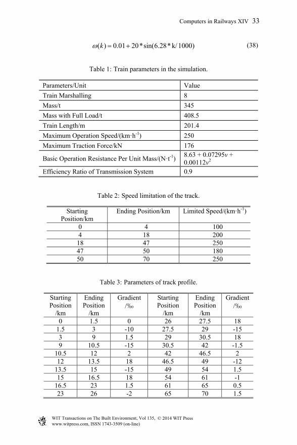
( ) 0.01 20*sin(6.28* k/1000)k (38)

Table 1: Train parameters in the simulation.

Parameters/Unit Value

Train Marshalling 8

Mass/t 345

Mass with Full Load/t 408.5

Train Length/m 201.4

Maximum Operation Speed/(km·h-1) 250

Maximum Traction Force/kN 176

Basic Operation Resistance Per Unit Mass/(N·t-1) 8.63 + 0.07295v + 0.00112v2

Efficiency Ratio of Transmission System 0.9

Table 2: Speed limitation of the track.

Starting Position/km

Ending Position/km Limited Speed/(km·h-1)

0 4 100 4 18 200

18 47 250 47 50 180 50 70 250

Table 3: Parameters of track profile.

Starting Position

/km

Ending Position

/km

Gradient /‰

Starting Position

/km

Ending Position

/km

Gradient/‰

0 1.5 0 26 27.5 18 1.5 3 -10 27.5 29 -15 3 9 1.5 29 30.5 18 9 10.5 -15 30.5 42 -1.5

10.5 12 2 42 46.5 2 12 13.5 18 46.5 49 -12

13.5 15 -15 49 54 1.5 15 16.5 18 54 61 -1

16.5 23 1.5 61 65 0.5 23 26 -2 65 70 1.5



Figure 5: Optimal speed profile offered by the planner.

Figure 6: Results of the tracking speed profile.

0 10 20 30 40 50 60 700

50

100

150

200

250

Sp

eed

(km

/h)

full powerpartial power

coasting

partial braking

full brakingspeed limit

0 10 20 30 40 50 60 70-300

-200

-100

0

100

200

Fo

rce

(kN

)

traction force

braking forceresistance force

0 10 20 30 40 50 60 70

0-101.5 -15218-15181.5 -2 18-1518 -1.5 2 -121.5 -1 0.5 1.5

（）Kilometer post km

0 1 2 3 4 5 6 7

x 104

-50

0

50

100

150

200

250

Distance(m)

Sp

eed

(km

/h)

Reference speed

System Output

Control Output

Observation of disturbance



Figure 7: Deviation of the tracking speed.

5 Conclusion

A new real-time controller of high speed train is proposed in this paper, which can improve punctuality of the train and reduce energy consumption simultaneously. With the help of the planner module, high speed train can get the optimal switching regimes along the whole journey section for the optimization objective of energy consumption minimization. Actually, if the train deviates the original planned speed profile due to commands for safety protection from the railway signal system, the planner module can recalculate a new optimal speed profile for punctuality constraint. Simulations show that the active disturbance rejection controller as the actuator can track the planned speed profile accurately. Future work will focus on the algorithm efficiency of the planner module to implement the optimal linkage within some acceptable time on the embedded processor, more proper arrangement of the transition process and parameters setting problem of the actuator module.

References

[1] Lee D., Milroy I., Tyler R., Application of Pontryagin’s principle to the semi-automatic control of rail vehicle, in Proceedings of the Second Conference on Railway Engineering, 1982: 233-236.

[2] Benjamin B., Long A., and Milroy I. et al., Control of railway vehicles for energy conservation and improved timekeeping, in Proceedings of the Conference on Railway Engineering, 1987: 41-47.

[3] Liu R., Iakov M., Energy-efficient operation of rail vehicles, in Transportation Research, Part A: Policy and Practice, 2003, 37(10): 917-932.

0 1 2 3 4 5 6 7

x 104

-2

-1

0

1

2

3

4

5

6

7

Distance(m)

Sp

eed

(km

/h)

Speed deviation



[4] Vu X., Analysis of conditions for the optimal control of a train, University of South Australia, 2006.

[5] Howlett P., Pudney P., Vu X., Local energy minimization in optimal train control, Automatica, 45(11): 2692-2698, 2009.

[6] Khmelnitsky E., On an optimal control problem of train operation, IEEE Transactions on Automatic Control, 45(7): 1257-1266, 2000.

[7] Zhu J., Li H., Wang Q., et al., Optimization analysis on the energy saving control for trains, China Railway Science, 29(2): 104-108, 2008. (in Chinese)

[8] Han J. Active disturbance rejection controller and its applications, Control and Decision, 1998, 3(1): 19-23 (in Chinese).

[9] Li S. H., Liu Z. G. Adaptive speed control for permanent-magnet synchronous motor system with variations of load inertia. IEEE Trans. On Industrial Electronics, 2009, 56(8): 3050-3059.

[10] Talole Sanjay E, Kolhe Jayawant P, Phadke Srivijay B. Extended-state-observer-based control of flexible-joint system with experimental validation. IEEE Trans. On Industrial Electronics, 2010, 57(4): 1411-1419.

[11] Wu D, Chen K. Design and analysis of precision active disturbance rejection control for noncircular turning process. IEEE Trans. on Industrial Electronics, 2009, 56(7): 2746-2753.

[12] Richard F., Suresh P., Raymond G., A survey of the maximum principles for optimal control problems with state constraints, SIAM Review, 37(2): 181-218, 1995.



the hierarchical real-time control of high speed trains for automatic · pdf...

Documents