1

The Generalized Method of Moments forElectromagnetic Boundary Integral Equations

Daniel Dault, Student Member, IEEE, Naveen V. Nair, Member, IEEE, Jie Li, Student Member, IEEE,Balasubramaniam Shanker, Fellow

Abstract—The Generalized Method of Moments (GMM) is apartition of unity based technique for solving electromagneticand acoustic boundary integral equations. Past work on theGMM for electromagnetics was confined to geometries modeledby piecewise flat tessellations and suffered from spurious internalline charges. In the present article, we redesign the GMMscheme and demonstrate its ability to model scattering fromPEC scatterers composed of mixtures of smooth and non-smoothgeometrical features. Furthermore, we demonstrate that becausethe partition of unity provides function and effective geometricalcontinuity between patches, the GMM permits mixtures of localgeometry descriptions and approximation function spaces withsignificantly more freedom than traditional moment methods.

Index Terms—Generalized Method of Moments, BoundaryIntegral Equations, Higher order discretization

I. INTRODUCTION

S Ignificant effort has been exerted in recent years towardconstructing discretizations of electromagnetic integral

equations that model the underlying continuous problem moreclosely than traditional low order approaches. The aim ofthese efforts is to obtain solutions with better fidelity to thecontinuous solution while significantly reducing the size ofthe descretized system and realizing commensurate savingsin computational cost. Most of the work to these ends hasfocused on one (or a combination) of three directions: higherorder current approximating function spaces that require fewerthan the traditional 10 degrees of freedom per wavelength,higher order geometry descriptions that more closely modelthe true continuous geometry, and mixtures of basis sets, e.g.mixing low order interpolatory basis sets with those derivedfrom asymptotic wave representations.

Moment methods that are higher order in both currentapproximation spaces and geometry representation have beena subject of intense development in recent years. Methodsfor higher order current representation have been traditionallybased either on hierarchical higher order functions residing inNedelec Spaces [1]–[4], or on variations of mapped higherorder polynomial tensor products [5]–[8]. By reducing thenumber of degrees of freedom per wavelength required todiscretize the integral operator, each of these methods re-alizes reductions in MoM system size. However, the phys-ical requirement that approximation functions must provide

D. Dault is with the Department of Electrical and Computer Engineer-ing, Michigan State University, East Lansing, MI 48824-1226 email: dault-dan@egr.msu.edu

N.V. Nair, J. Li and B. Shanker are with the Department of Electrical andComputer Engineering, Michigan State University

current continuity between discretization subdomains placesstrict limitations on the types of basis functions that maybe employed, and means that the boundary integral operatorsgenerally must be discretized using a single class of basisfunction, e.g. only polynomials. Some methods for mixinghigher order polynomial bases with other basis classes havebeen developed (e.g. singularity type bases in [9]), but thesealso require that the basis set be designed to enforce currentcontinuity.

Closely related to the issue of continuity in basis functionset is that of continuity in geometry description. Higher ordersurface descriptions for moment methods are generally basedon smooth polynomial surface parameterizations [10], whichhave difficulty accurately modeling geometrical singularitiessuch as edges and tips. Recently, representations using Non-rational B-Splines (NURBS) have been developed [11], [12].A bottleneck with both of these methods is enforcing geo-metrical continuity at abutting patch edges. As with currentapproximations, this generally forces the use of the sametype approximating function for the parameterization of eachsubdomain.

The GMM is a partition of unity method that decomposesthe scatterer surface into overlapping subdomains, termed“patches”. As in the Generalized Finite Element Method [13],[14], the partition of unity serves to decouple approximationfunction descriptions in neighboring subdomains. Consequen-tially, GMM is able to easily incorporate higher order basissets, higher order/mixed geometry descriptions, and arbitrarymixing of approximation function spaces. This flexibility inapproximation functions occurs because interpatch continuityis provided not by the approximating functions themselves,but by the partition of unity. This lifting of the continuityconstraint on the basis functions permits substantially morefreedom in the types of approximation function spaces thatmay be employed; additionally, it allows mixing of differentapproximation spaces in adjacent subdomains over the surfaceof the scattering body. Thus, in the GMM, basis sets maybe freely chosen to match local current ansatz. The parti-tion of unity scheme also allows blending of different func-tional geometrical descriptions in the overlap region betweensubdomains, effectively providing geometrical continuity andpermitting the use of distinct geometry parameterizations onneighboring subdomains. This implies that geometry param-eterizations from entirely different spaces, e.g. polynomials,conics, and flat tessellations, may be utilized in the samesimulation while maintaining effective geometrical continuity.

Although partition of unity methods have been widely em-

arX

iv:1

401.

5418

v1 [

phys

ics.

com

p-ph

] 2

1 Ja

n 20

14

2

ployed in finite elements to address some of the challenges inbasis function and geometrical continuity [15]–[18], extensionof these methods to integral equations has been limited, in partbecause defining meaningful partitions of unity on arbitrarytwo dimensional manifolds residing in R3 is a nontrivial prob-lem. Nonetheless, the Partition of Unity Boundary ElementMethod (PUBEM) [19] has been developed, primarily forthe solution of two dimensional acoustic Helmholtz scatteringproblems. In PUBEM, traditional interpolating approximationfunction spaces are enriched with asymptotic plane wavebases for electrically/acoustically large simple scatterers in twodimensions [20], [21], and a sphere in three dimensions [22].A similar approach is taken in [23], [24], wherein stationaryphase methods are applied to acoustics and electromagneticsproblems using asymptotic representations on electrically largesmooth geometries. The approach in the present paper issignificantly more general than these approaches because itapplies to vectorial electromagnetics problems on arbitrarilyshaped scatterers in three dimensions. The approximationspaces utilized may be arbitrary mixtures of basis functionsincluding, but not restricted to, the plane-wave and asymptotictype expansions employed in the PUBEM and [24].

Finally, we note that the Generalized Method of Momentsmay be technically classified as a quasi-meshless method.Meshless methods have traditionally been confined to the finiteelement community, especially in the field of mechanics andmechanical engineering (e.g. [25], [26]), although there hasbeen increasing interest toward applying such methods to com-putational electromagnetics, primarily in the context of quasi-static problems [27]–[29], and generalized finite elements,[30], [31]. To the authors’ knowledge, the only applications ofmeshless methods to high frequency electromagnetic integralequations, excepting GMM and the references in the precedingparagraph, are implementations of the traditional MovingLeast Squares (MLS) method [32], [33] and the work in[34], in which both a MLS-based collocation scheme and anintegral transform-based approach are given. The GeneralizedMethod of Moments is distinct from these methods in thatit incorporates ideas from mesh-free discretization (node-based primitives, partitions of unity) to effect localization ofgeometry and approximation functions, but then marries theseideas with the large variety of moment method basis sets thathave been developed by the electromagnetics community overthe last five decades.

The present work provides a unified prescription for thealgorithmic development and implementation of the Gen-eralized Method of Moments for arbitrary PEC scatterers.The GMM for electromagnetic integral equations was firstpresented in [35] for piecewise flat tessellations and has beenextended to low-order (tessellated) Muller formulations fordielectrics [36] and a higher order smooth formulation foracoustics [37]. In this work, we extend electromagnetic GMMto geometries composed of mixtures of features includingflat regions, tessellations, polynomial smooth patches, sharptips, bodies of revolution, conic sections, etc. The inclusionof local smooth geometry descriptions removes one majorhurdle encountered in the piecewise flat approach in [35],which is the appearance of spurious line charges at boundaries

between non-coplanar triangles. By introducing either smoothlocal geometry parameterizations or subdomain basis setsthat cancel line charges by construction, the present workavoids line charges altogether. Preliminary work on smoothlocal parameterizations and hybridizations with non-smoothgeometrical descriptions for GMM is contained in [38], [39],and [40].

Specific contributions of this paper are:

• A framework for arbitrarily mixing different classes ofbasis functions over the surface of a PEC scatter.

• A geometrical hybridization scheme wherein variousfunctional geometry descriptions may be combined andblended in a single problem.

• A smooth, higher order geometry representation frame-work for representing arbitrary curved geometries.

• Hybridization with tessellations and introduction of “sub-patch” basis sets capable of handling geometrical singu-larities.

• Algorithms for automatically assigning approximationfunction types and local geometry descriptions based onlocal physical characteristics of the scattering geometry.

• Results demonstrating the flexibility of the method onseveral test scattering problems.

The scattering results are designed to demonstrate mixingof geometry descriptions and basis function classes, and thecorresponding reduction in system size. To address largerproblems, the method will be hybridized with the MultilevelFast Multipole Method [41] in future work.

The remainder of the paper is organized as follows. Sec-tion II briefly outlines the problem under consideration. Theformulation of GMM for arbitrary PEC scatterers, includingconstruction of patches starting from point clouds, the par-titions of unity, local geometry parameterizations, local basisfunctions, and the evaluation of matrix elements, is detailed inSection III. Results validating the method against a referencecode and demonstrating application of the method to severalrepresentative geometries are presented in section V. Finally,Section VI provides some concluding remarks and futuredirections.

II. PROBLEM STATEMENT

The problem of interest is the computation of the scatteredfields Es(r),Hs(r) due to a plane wave, characterizedby the triad ki,Ei(r),Hi(r), impinging on a PEC objectresiding in free space. The scatterer boundary Ω is equippedwith a unit normal n(r) defined for all r ∈ Ω except at afinite number of geometrical singularities (e.g. corners, tips,edges, etc.). The boundary integral formulation we employ isthe Combined Field Integral equation (CFIE):

αn(r)× n(r)×Ei(r) + (1− α)n(r)×Hi(r) =

−αn(r)× T j(r) + (1− α)(I −K) j(r)(1)

where I is the identity operator, 0 ≤ α ≤ 1 is a constantweighting factor, and the operators T and K are given by:

3

T j(r) = −n(r)×

[jkη0

4π

∫Ω

dr′g(r, r′)j(r′)

+jη0

4πk

∫Ω

dr′∇∇g(r, r′) · j(r′)

]K j(r) =

1

4πn(r)×

∫Ω

dr′∇g(r, r′)× j(r′)

(2)

Here, j(r) = n(r) × Hi(r) + Hs(r) is the inducedsurface current, g(r, r′) is the free-space Helmholtz Green’sfunction, k is the propagation constant, and η0 is the intrinsicimpedance of free space. An ejωt dependence is assumed andsuppressed. To construct a moment method system, the surfacecurrent is discretized in terms of a set of basis functions asj(r) =

∑Ns

n=1 anfn(r) and the discretized operators in (2) aretested with a set of functions fm(r),m ∈ [1, Ns] in the usualfashion.

III. FORMULATION

Although many details of the construction of GMM forpiecewise flat tessellation and scalar acoustic equations aregiven in [35] and [37], we include a detailed discussionhere because these techniques have not been developed forelectromagnetic integral equations on smooth surfaces, andbecause the present method differs in several respects fromprevious work.

The GMM is constructed via a decomposition of the mani-fold Ω into overlapping subdomains, termed “patches”, and de-noted by the set Ωi. Each patch Ωi comprises four elements:1) a set of nodes Ni, 2) a local geometrical parameterizationGi and associated projection plane Γi, 3) a partition of unityψi, and 4) a local approximation function space, fk(r). Inthe following section, we first develop patch definitions anddefine the partitions of unity, which decouple geometry andapproximation functions spaces on neighboring patches. Wethen describe in some detail the design of the local geometrydescriptions and basis sets. The set of patches Ωi may beconstructed in several ways depending on the level of a prioriinformation that is known about the surface. We employ thefollowing approach, which only requires an oriented pointcloud as a starting point.

A. Neighborhoods from Point Clouds

To begin, we require only that Ω be sampled with a discreteset of Nm nodesN .

= ni, i = 1, 2, 3, . . . , Nm residing in R3

and equipped with a connectivity map in the sense of nearestneighbors (note that standard simplicial tessellations implicitlycontain this information). Denote by Ni the neighborhood ofthe ith node, which is initially defined as the set containingni and the set of its nearest neighbors N i

.= Ni/ni as

specified by the connectivity map. Additionally, we require anorientation, specified by a normal defined at each ni. Thesenormals may be a priori provided, or may be obtained usinga classical normal estimation routine, e.g. [42]. In the casewhere a node occurs at a geometrical singularity such as atip or corner, the normal is not uniquely defined; in GMM

such nodes are flagged as “singular” and are handled using amodified algorithm, which is discussed in a later section. Forthe remainder of this section, we assume that the geometry isfree from singularities.

Given the node list N and corresponding normals, for eachni we define a subdomain Ωi centered on ni and bounded byN i. Each Ωi is termed a “patch primitive”. We label the set ofpatch primitives that neighbor Ωi as ΩN i

.= Ωj |nj ∈ N i,

i.e. ΩN iis the set of all patch primitives associated with nodes

that neighbor ni, but not including Ωi. By definition each Ωioverlaps with all patches in ΩN i

.Although the initial set of patches Ωi is defined about ev-

ery node in N , it is often advantageous to merge neighboringprimitives into larger patches, e.g., if the patch primitives aresmall with respect to the characteristic scale of the problemor form part of the same surface of revolution. We denote theset of merged patches as Ωi, with each final patch definedas a union of some subset of patch primitives: Ωi

.= ∪Nk

k=1Ωk,with Ωk an Nk-dimensional subset of Ωi. After merging, thefinal patches may be associated with much larger collections ofnodes, with neighborhoods Ni and patch neighbor sets ΩN i

updated accordingly. As patch merging algorithms dependon local geometric characteristics, we defer discussion of asample merging algorithm until section IV-B. Because thereis no formal distinction between merged patches and patchprimitives (they are two instances of the same type of object),we drop the hat notation for the remainder of the paper anduse the set Ωi to denote the set of all patches for a givenscatterer, primitive or otherwise.

B. Partition of Unity

Subordinate to each Ωi, we define a partition of unityfunction ψi(r) with suppψi(r) = Ωi with the propertythat

∑i ψi(r) = 1∀r ∈ Ω. These partitions of unity serve

to decouple neighboring patches, so that any surface functionφ(r), r ∈ Ω may be reconstructed as φ(r) =

∑i ψiφi(r),

where the subsectional functions φi(r) are given by φi(r) =χiφ(r), with χi the characteristic function of patch Ωi. InGMM, partition of unity is enforced using an approach basedon traditional Shepard Interpolation [43], which takes theform:

ψi(r) =ψi(r)

ψi(r) +∑j ψj(r)

(3)

in which ψj(r) is a local shape function with compactsupport on patch Ωj , and ψj(r) is the set of local shapefunctions defined on the set ΩNi

of patches that neighbor Ωi.The choice of local shape function depends on the problemtype, and may include simplex type functions, smoothly de-caying exponentials, polynomial-based functions, etc. In thepresent work, a simplex-based partition of unity is utilized.Figure 1 illustrates the blending of basis function spaces viathe partition of unity in one dimension. These concepts extenddirectly to functions and patches defined on two dimensionalmanifolds, and also effectively permit blending of differentgeometry descriptions in the overlap region between patches.

4

1 2 3 4x

1.0

0.5

0.5

1.0

1.5

(a)

1 2 3 4x

1.51.00.50.00.51.01.52.0

(b)

1 2 3 4x

1.51.00.50.00.51.01.52.0

(c)1.5 2.0 2.5 3.0 3.5 4.0

x

0.2

0.4

0.6

0.8

1.0

(d)

1 2 3 4x

1.0

0.5

0.5

1.0

1.5

(e)

0 1 2 3 41.51.00.50.00.51.01.52.0 0

5-

10-

15----

(f)

Fig. 1: Blending of approximation spaces on overlappingdomains via the partition of unity for a 1D signal. (a)A trial function f(x) = .2(x − 2)3 + .3 on the intervalΩ : 0 ≤ x ≤ 4. (b) Interpolation of f(x) using linearinterpolatory hat functions Ti(x) = T (x− .5i) on subintervalΩ1 : 0 ≤ x ≤ 3 such that f1(x) = χ1(x)

∑i aiTi(x),

χ1(x) = 1, x ∈ Ω1; 0, x 6∈ Ω1 . (c) Interpolation off(x) using a third order Legendre polynomial set Pn(x),n = 0, 1, 2, 3 on subinterval Ω2 : 2 ≤ x ≤ 4 such thatf2(x) = χ2(x)

∑3n=1 anPn(x − 3), χ2(x) = 1, x ∈ Ω2,

0; x 6∈ Ω2. (d) Partitions of unity ψ1(x) and ψ2(x). (e)interpolations of f(x) multiplied by partitions of unity asf1(x)ψ1(x) in Ω1 and f2(x)ψ2(x) in Ω2. (f) Reconstructedfunction f(x) = f1(x)ψ1(x) + f2(x)ψ2(x) (left axis) andabsolute reconstruction error (right axis). Through the action ofthe partition of unity, the representations f1(x) and f2(x) aresmoothly blended in the overlap region, 2 ≤ x ≤ 3, and theapproximation error transitions smoothly between the linearand Legendre interpolations.

C. Local Geometry Parameterization

In this section, we develop methods for constructing localsurface geometry descriptions on each patch in Ωi. Theselocal surface descriptions are superposed as

⋃i Ωi to recreate

the original geometry. This scheme admits a wide variety in thechoice of local geometry parameterization. We now describelocal geometry construction for both smooth and nonsmoothregions of the scatterer.

From the definition of patches above, each patch Ωi containsa set of nodes Ni = nk located at positions rk andequipped (in the smooth case) with normals nk. Localsmooth surface parameterization for Ωi proceeds as a two-stepprocess. First, a “projection plane” Γi is defined such that theplane normal ni is the average of all subordinate node normals:

ni =

∑k nk

|∑k nk|

(4)

The plane Γi is uniquely defined by its normal and apoint rci (defined with respect to the global origin) throughwhich the plane passes; generally, this point is taken as theaverage of the locations of nk, although it may be chosenotherwise depending on the requirements of different geometryparameterizations.

Once the plane Γi has been defined, an orthogonal localcoordinate system (u1, u2, u3) is constructed as follows. First,the altitude direction is taken parallel to ni: u3 = ni. Theu1 direction is defined in the direction of maximum patchdimension, max|rkb − rjb|, where the b subscript indicatesa boundary node. The remaining coordinate direction is thendefined as u2 = u3 × u1. The local coordinate system isdefined with respect to a local origin located at rci .

Upon establishment of the local coordinate system, a pa-rameterized manifold Λi passing through the nodes nk isdefined. This parameterization takes the form:

Λi.=r ∈ R3 | r(u1, u2) = ri(u1, u2) + rci,

ri(u1, u2) = u1u1 + u2u2 + wi(u1, u2)u3

(5)

where ri(u1, u2) indicates a local position vector pointingfrom the (u1, u2, u3) origin to the parameterized surface. Thedomain of the parameterization is restricted to a polygon inthe projection plane Γi that bounds the projection PΓi

(Ni) ofthe node set Ni into Γi: u1, u2 ∈ PΓi(Ni). We denote the typeof parameterization on patch Ωi by Gi. The altitude functionwi(u1, u2) may be taken as any well-behaved function of(u1, u2). The conditions for wi(u1, u2) to be well-behavedare that 1) it is single-valued, 2) its Jacobian is amenable tointegration through standard numerical quadrature techniques,and 3) it maintains an appropriate degree of geometricalcontinuity with neighboring patch descriptions. As long asthese conditions are satisfied, different local geometry param-eterizations may be used on different patches, and the choiceof parameterization Gi my be matched to local geometricfeatures, e.g. a BoR description for rotationally symmetricsurface regions, corner elements for edges and tips, Beziersurfaces, etc. The mixing of multiple surface descriptionsgeneralizes the work in [40], which hybridized polygonaltessellations with smooth polynomial surface descriptions.Figure 2 summarizes patch neighborhood and local geometryconstruction for smooth geometries.

1) Smooth Polynomial Geometry Parameterization: Al-though any parameterization satisfying the conditions stated inthe previous section may be utilized to define patch surfaces,it is desirable to have a default parameterization scheme forsurfaces where no a priori surface description is known apartfrom the node locations and normals. To effect this scheme,following [44] we use a polynomial surface description for theparameterized manifold Λi:

ri(u1, u2) = u1u1 + u2u2 + Pgi (u1, u2)u3 (6)

where Pgi (u1, u2) is as a degree g tensor product of poly-nomials in u1 and u2:

5

(a) (b)

(c) (d)

(e) (f)

Fig. 2: Smooth Patch Geometry Parameterization Procedurefor patch Ωi: (note: for clarity, subscripts i are dropped onvector quantities) (a) Start with an oriented point cloud ,and (b) define a neighborhood Ni of nearest neighbors aboutnode i. (c) Define a projection plane Γi with normal equal toaverage of all node normals and specified by a point rc thatuniquely defines an origin of coordinates. (d) Construct a localorthogonal u1, u2, u3 coordinate system. (e) Take projectionof points in Ni into Γi to define the support of the patch inthe u1, u2 plane. This projection is denoted PΓi

. (f) Obtain asmooth parameterization to define the local patch surface.

Pgi (u1, u2) =∑|α|≤g

cαuα11 uα2

2 (7)

Here we have employed standard multi-index notation α .=

(α1, α2), |α| = α1 + α2 for compactness. The coefficientscα are obtained via least-squares fit. The geometrical fidelityof Λi to the original node locations is controllable by thedegree g and the tolerance in the least squares algorithm.By defining Λi as a polynomial function Pgi (u1, u2), Λi isensured to lie the space Cg of g-differentiable functions. Thisproperty is important in evaluating field integrals because basisfunctions in the GMM scheme inherit the differentiability ofthe geometry parameterization.

2) Handling of Geometrical Singularities: In the casewhere a patch contains nodes that lie on geometric sin-gularities, a modified geometry parameterization method isemployed. If an analytical description of geometry in theneighborhood of singularity is known, as with a conical tip orstraight edge, a custom geometrical description that correctlyhandles the singularity may be constructed. Alternatively, astandard triangular tessellation may be defined on the setof nodes adjacent to (and including) the singular nodes.Appropriate basis sets are then defined on the tessellation thatcorrectly capture the behavior of currents and charges nearthe singular feature. Although the design of these functions isoutside the scope of this paper, several such basis functions

Fig. 3: Tangent and normal vectors associated with a paramet-ric patch surface

have been developed (the most prevalent being the RWG classof functions) that can be easily incorporated into the GMMframework.

3) Vector Calculus on Parametric Surfaces: Here, webriefly define quantities required to do vector calculus on theparametric surface specified by r(u1, u2). Vectors tangentialto the surface are expressed as t = aru1 + bru2 , where a, bare scalar coefficients and the basis vectors ruj

, j = 1, 2are defined by ruj

.= ∂r/∂uj . Note that the tangent basis

vectors are not normalized, and in general do not need to beorthogonal. For the types of parameterizations used in thispaper, the basis vectors are given explicitly by:

ru1= u1 +

∂w(u1, u2)

∂u1u3

ru2= u2 +

∂w(u1, u2)

∂u2u3

(8)

The unit normal is given in terms of these tangent basisvectors as n = (ru1

× ru2)/||ru1

× ru2||. Figure 3 shows

ru1, ru2

and n on the parametric surface.For the purposes of integrating and taking derivatives with

respect to the parametric coordinates (u1, u2), it is necessary todefine notions of differential length and area on the parametricsurface. To do so, a transformation matrix called the “metrictensor” is defined as:

g =

[ru1· ru1

ru1· ru2

ru2 · ru1 ru2 · ru2

](9)

Traditionally, components of the metric tensor are indexedusing lowered indices gij . The inverse of the metric tensorg−1 is used in expressions involving derivatives, and thecomponents of g−1 are referenced using raised indices gij .The differential surface area element is given by dS = Jdu =Jdu1du2 where the Jacobian is J =

√det(g), with det(g)

the determinate of the metric tensor. Finally, the surfacedivergence of a vector function f(r(u1, u2)) on the surfacewith respect to the parametric coordinates is:

∇s · f(u1, u2) =

2∑i,j

gij∂f

∂ui· ruj (10)

This expression is used to compute the divergences ofsurface currents required in the T operator of equation (2).For further development of these concepts in the context ofelectromagnetics, we refer the reader to [45], [46].

6

Fig. 4: Entire Patch Basis Function

D. Local Basis Functions

Next, we develop local basis function descriptions. GMMpatches may incorporate either entire patch (EP) bases withsupport over the entire patch, or sets of sub patch (SP) baseswith support smaller than the entire patch.

1) Entire Patch Basis Functions: The general entire patchvector basis function is given in terms of local coordinates as:

fi,k(r) =fk,1(u1, u2)ru1(u1, u2)

+ fk,2(u1, u2)ru2(u1, u2)(11)

so that the unknown surface current on patch Ωi is expressedas:

ji(r) = ψi(r)

Ni∑k=1

akfi,k(r) (12)

Here, ψi(r) is the partition of unity on patch Ωi, the vectorsru1

and ru2are tangent vectors to the surface as defined in

section III-C3, and the weighting functions f1,k(u1, u2) andf2,k(u1, u2) may be chosen from any set of functions thatlead to convergent integrals on Λi. Examples of such choicesare hierarchical polynomials, plane waves, body of revolutionfunctions, etc.

To construct EP basis functions, first a canonical minimumbounding shape is defined that encloses the projection PΓi

ofthe patch node set Ni onto the local projection plane Γi. Thechoice of bounding shape depends on the patch type and shape.Rectangles are generally employed for mapped polynomialfunctions, circles for BoR, etc. Once the appropriate boundingshape is assigned, the component basis functions fk,1(u1, u2)and fk,2(u1, u2) are defined on its interior and restricted tothe domain included in PΓi

. Finally, these basis functions arelifted onto the parametric surface as in (11). This arrangementis illustrated in figure 4.

2) Sub-patch Basis Functions: GMM can also easily in-corporate multiple basis functions on a single patch with sub-patch support, so called sub-patch (SP) bases. This may be in-terpreted as defining an EP basis function as f(r) =

∑j fj(r),

Fig. 5: Illustration of sub-patch basis function arrangementwith projected PU

with fj(r) a set of approximation functions with supportsmaller than suppΩi. The requirements on SP bases are thatthey introduce no line charges interior to the patch, and thatthey possess a normal component at the patch edges. Due tothe partition of unity, the normal component is only required tobe finite, and need not satisfy any explicit continuity constraintacross patch boundaries.

Sub-patch bases may be defined on the projection plane andprojected onto the parameterized surface as with EP bases;alternatively, SP functions may be defined directly on a tes-sellation of the point cloud as in a traditional Moment Methoddiscretization. Likewise, the partition of unity is defined eitheron the projection plane Γi and then lifted onto the true surface,or is defined directly on the tessellation itself. Defining sub-patch bases in this way allows most basis function typesfrom existing tessellation-based Moment Method codes to bedirectly used in the GMM scheme with minimal alteration.Figure 5 shows an example sub-patch tessellation.

To illustrate the manner in which sub-patch bases areimplemented in the GMM scheme, we detail the constructionof a tessellated patch with Rao-Wilton-Glisson (RWG) [47]basis functions. RWG functions are defined as usual on thetessellated surface, or equivalently, on the projection planeand lifted onto the surface. A simplicial partition of unityfalls naturally into the RWG framework and is defined sothat it takes a value of unity in all interior triangles and fallslinearly to zero in boundary triangles. To provide the necessarynormal component at the patch edge, a half-RWG functionis defined across exterior patch boundaries. Although half-bases are generally avoided in RWG discretizations becausethey introduce line charges, this difficulty is avoided in GMMbecause the PU forces the function to zero at the patch edge.This property of the PU applies to all GMM basis functions,and renders the basis set on a patch charge neutral, regardlessof whether the functions are EP or SP. Figure 6 shows interiorand boundary RWG basis functions, and the PU’s removal ofthe boundary line charge.

7

(a) (b)

PU

(c)

Fig. 6: Design of local RWG basis set with normal continuityacross patch boundaries: (a) Internal RWG basis functions,(b) Added external half-RWG functions to provide a normalcomponent at patch edge, and (c) Simplex-based partition ofunity forces the half-RWG function to zero at patch boundary,removing the line charge.

3) Default EP/SP Basis: As with local geometry descrip-tions, it is advantageous to have default basis function typesthat are utilized when a current ansatz is not available ordifficult to obtain. A straightforward choice of an EP basisfunction is:

f1(u1, u2) = φβ(u1, u2)ru1

f2(u1, u2) = φβ(u1, u2)ru2

(13)

where φβ(u1, u2).= Pβ1(u1)Pβ2(u2) is a product of two

Legendre polynomials of degrees β1 and β2, and the entirepth order representation on patch Ωi is constructed as:

ji(r) = ψi(r)

2∑l=1

∑|β|≤p

aβ,lφβ(u1, u2)rul(14)

More complex polynomial bases may be constructed, e.g.one which explicitly enforces a surface Helmholtz decompo-sition, as in [35]. However, we have found that the minimaltensor product of Legendre polynomials in (14) generallyprovides better matrix conditioning than other choices ofpolynomial basis functions for the same order. Furthermore,since GMM provides current continuity between patches bydesign, it is not necessary to use the modified Legendre basesor hierarchical bases often employed in higher order mappedmethods [6], [10].

With the influence of the partition of unity, the surface

current approximation for the default EP basis spans the space:

f1(u1, u2) ∈ spanψi(r)(φβ(u1, u2)ru1)

+ψi(r)(φβ(u1, u2)ru2)

|β| ≤ p(15)

As described in section III-C, when geometrical singularitiessuch as sharp tips or edges are present, a smooth geometryparameterization and polynomial EP basis cannot be used.Therefore, in these situations, we default to a surface tessel-lation supporting a SP RWG basis as detailed in III-D2. Theproperties of these functions have been extensively developed[47] and will not be repeated here.

Finally, we explicitly show how the partitions of unity andhalf-RWG basis functions are constructed in the case of Legen-dre (EP-type) and RWG (SP-type) patches that overlap. Figure7.a shows the partition of unity ψRWG = ψRWG/(ψRWG +ψLeg) and location of half-RWG basis functions for theRWG patch, and Figure 7.b shows the partition of unityψLeg = ψLeg/(ψRWG + ψLeg) on the Legendre patch. Thesub-partition of unity ψRWG on the RWG patch is defined ona triangle-by-triangle basis as:

ψRWG =

1, nbd = 0

ξ, nbd = 1

1− ξ, nbd = 2

(16)

where nbd is the number of triangle nodes on the patch bound-ary (in the overlap region) and ξ is the simplex coordinateassociated with the exterior node if nbd = 1 or the interiornode if nbd = 2. A similar definition may be used to constructψLeg .

IV. IMPLEMENTATION DETAILS

In this section, we discuss some practical details of evalu-ating GMM matrix elements and give sample algorithms forpatch merging and basis function assignment. Each of thesetasks is nontrivial, and investigations of the most efficient andeffective methods for specific types of problems are subjectsof ongoing investigation. The integration methodology pre-sented is sufficiently general that it may be used for mostGMM integrations, although more specialized rules could bedeveloped for specific basis function types. The integrationsand algorithms developed here are used to generate all of theresults in section V.

A. Matrix Elements

We devote this section to a brief discussion of the practicalevaluation of GMM matrix elements. Using the surface param-eterizations from Section III-C and the differential geometryquantities from Section III-C3, the tested scattered electricfield portion of (2) becomes :

8

(a)

(b)

Fig. 7: Graphical depiction of partitions of unity for overlappedRWG and Legendre patches. (a) Partition of unity ψRWG andhalf-RWG basis functions for an RWG patch. (b) Partition ofunity ψLeg for a Legendre patch.

−jkη0

4π

∫Di

duiJi(ui)ψi(ui)fi,m(ui)

·∫Dj

du′jJj(u′j)g(ri(ui), rj(u

′j))ψj(uj)fj,n(u′j))

+jη0

4πk

∫Di

duiJi(ui)∇s · (ψi(ui)fi,m(ui))∫Dj

du′jJj(u′j)g(ri(ui), r

′j(u′j))∇′s · (ψj(uj)fj,n(u′j))

(17)

where we have employed the standard derivative transfersin the Φ portion of the T operator. The tested magnetic fieldintegral equation portion of (2) is:

1

4π

∫Di

duiJi(ui)ψi(ui)fi,m(ui)ψj(uj)fj,n(uj)−∫Di

duiJi(ui)fi,m(ui) · n(r(ui))×∫Dj

du′jJj(u′j)∇g(ri(ui), rj(u

′j))× ψj(uj)fj,n(u′j)

(18)

were ul = (u1, u2) ∈ Γl denotes the local transversecoordinates for patch l, Jl is the Jacobian as defined in sectionIII-C3, and Dl ∈ Γl is the domain of integration in theprojection plane. If the projection PΓl

(Nl) of the nodes in Nlis a canonical integration domain, e.g. a regular polygon, thenan appropriate quadrature rule can be used to integrate overthe entire projection. For instance, radial/angular rules are usedfor BoR patches. In the general case where the projection is

Fig. 8: (a) Graphical representation of PΓl(Nl) and (b) con-

struction of triangular integration subdomains. The domain ofintegration is Dl = ∪iTi.

not bounded by a canonical shape, we perform a triangulationof PΓl

, e.g. using Delaunay or another method. Figure 8illustrates this process. Subdividing the domain of integrationin this way allows the use of well-developed integration rulesfor triangles (including singularity rules), and the total integralis the sum of integrations over subtriangles. It is important tonote that not every node in PΓl

needs to be used in defining thetriangulation: if the patch is large, some subset of the nodesmay be used to lessen the integration cost, as long as the patchboundaries are correctly handled.

B. Automated Patch Construction

For large, complex geometries, it is necessary to auto-mate the processes of patch construction including merging,geometry parameterization, and basis function assignment.The following are two sample algorithms for merging andgeometry/basis selection.

1) Algorithm for Patch Merging: Using the procedure fromsection III-A, patch primitives are assigned in the initialpass. To reduce the number of degrees of freedom in theMoM system, it is often advantageous to merge patches ifneighboring primitives share common geometrical features,e.g. are part of the same body of revolution or fall on asufficiently smooth portion of Ω. Given the definition of Ωi asa collection of nodes, merging and or splitting may be simplydone by operating on the sets Ni. Algorithm 1 illustrates aprocedure for merging; splitting may be done in a similarfashion. Criteria for merging are tied both to patch size andpatch mean curvature, which is approximated via deviation ofnormals as shown in Algorithm 1.

At the end of the merging process, the final set of mergedpatches is designated Ωi. Algorithm 1 is a simplified versionof the actual merging algorithm used in the present GMMcode. In practice, additional higher level merging conditionalsare also used that, for instance, favor convex patch boundariesover concave boundaries, attempt to maintain equal patchsizes over the entire geometry, and group patches with similarcharacteristics, such as edge singularities or small curvature.

2) Automated Geometry and Basis Assignment: Algorithm2 illustrates automated assignment of local geometry descrip-tions G, basis function types b and (where applicable) ordersg using using tessellations, BoR surfaces, and polynomialsmooth surfaces for geometry parameterization and RWG,BoR, polynomial, and plane wave bases. Any geometry orbasis function class valid for the GMM framework may be

9

1: Define maximum normal deviation εn tolerance2: Define maximum average normal deviation εd tolerance3: Define maximum patch diameter Dm

4: for each patch primitive Ωi ∈ Ωi do5: for each nj ∈ Ni (corresponding to primitive Ωj do6: if nj · ni > (1− εn) then7: Define candidate merged neighborhood:

Nl = Ni⋃Nj . Designate the number of nodes in

Nl as M .8: Compute new average patch normal

nl =(∑M

k=1 nk)/|∑Mk=1 nk|

9: Compute merged patch maximum diameterD = max|rna

− rnb|, na, nb ∈ Nl

10: if D ≤ Dm then11: Compute average deviation ∆nl from patch

normal nl as: ∆nl.= 1

M

∑Mk=1 nl · nk

12: if ∆nl ≤ εd then13: Merge Ωi, Ωj:14: Ni ← Nl15: Ωi ← Ωi\Ωj16: end if17: end if18: end if19: end for20: end for

Algorithm 1: Automated patch merging

included in the algorithm with the proper conditionals. Thepresent code implementing GMM is written in a highly mod-ularized fashion that facilitates easy addition of new geometryand basis function types.

Algorithms 1 and 2 are used to discretize all of the scatterersin the results section.

V. RESULTS

In this section, we provide results that illustrate hybridiza-tion of geometry and basis types and verify the accuracy andflexibility of the method. First, we utilize a representation testto demonstrate the hybridization of multiple basis types inthe reconstruction of an analytical function. We then provideseveral scattering results, each with a different mixture ofbasis function types and orders defined on patches withvarying local geometry descriptions. Throughout the resultssection, the algorithms detailed in Section IV-B are used toautomatically assign local geometrical descriptions and surfacecurrent approximation spaces that are matched to solutionansatzes for the continuous problem. Doing so gives accuratesolutions with significant reductions in the numbers of degreesof freedom relative to a reference CFIE-RWG code.

We begin with a representation (Gram) test in which aquadratic vector function f(x, y) = (x−.5)2x is reconstructedon a flat 1m×1m plate using a mixture of a 2nd orderLegendre polynomials defined on smooth patches and RWGfunctions defined on a triangular tessellation. Figure 9 showsthe discretization and reconstruction error for three cases.

1: Define maximum patch normal deviation εd for smoothsurface description

2: Define maximum patch normal deviation for plane wavebasis εp

3: Define minimum patch diameter for plane wave Dp

4: for each final patch Ωi do5: Compute average deviation ∆ni from average patch

normal ni as: ∆ni.= 1

M

∑Mk=1 ni · nk

6: if ∆ni > εd then7: G: triangular tessellation8: b: RWG Basis9: else if Rotationally Symmetric Patch then

10: G: Axisymmetric BoR representation11: b: BoR Basis12: else13: G: Local smooth approximation to Ωi.14: if ∆ni < εp && DiamΩi > Dp then15: b: Plane Wave Basis16: else17: b: Polynomial Basis of order g18: end if19: end if20: end for

Algorithm 2: Automated geometry and basis assignment

Reconstruction error is taken as the pointwise absolute error(abs err)= |f(x, y)−f(x, y)|, where f(x, y) is the reconstructedfunction.

First, as a reference, we interpolate the analytical functionf(x, y) using the standard linear RWG basis on a triangular tes-sellation with maximum edge length .07m. This discretizationis shown in figure 9.a. Figure 9.b shows the reconstructionerror using the all-RWG basis set. As one would expect,the error is highest at the edges where the RWG functionscannot reconstruct the normal component, and lowest wherethe argument of f(x, y) goes to zero (at x = .5m). The purposeof this result is to provide a reference error level for RWGdiscretization for case 3, in which RWG and Legendre basesare mixed.

Figures 9.c and 9.d show discretization and reconstructionerror for an all-Legendre polynomial basis of second order.Because the basis set is polynomial complete to the sameorder as f(x, y), the reconstruction is perfect to machineprecision everywhere on the plate. Most significantly, thereconstruction is perfect even in the overlap regions betweenpatches where the partition of unity provides the continuity andblending between basis sets on neighboring patches. Withoutthe partition of unity, there would be significant error in theoverlap regions.

In figure 9.e, a .25m × .25m tessellated patch with RWGfunctions is placed in the center of the plate, while the outerboundary is discretized using flat patches supporting secondorder Legendre polynomials. Figure 9.f shows the reconstruc-tion error for the mixed RWG/Legendre basis set. In this case,the error in the RWG patch matches that from the center of the

10

(a) (b)

(c) (d)

(e) (f)

Fig. 9: Reconstruction error for a function f(x, y) = (x−.5)2xusing three different basis sets: all-RWG, all-Legendre, mixedRWG/Legendre. (a) All-RWG discretization, (b) All-RWGreconstruction error, (c) All-Legendre patch discretization (2ndorder Legendre polynomials) (d) All-Legendre reconstructionerror, (e) Mixed RWG/Legendre discretization (2nd order Leg-endre Polynomials), (f) Mixed RWG/Legendre reconstructionerror.

plate in figure 9.b. Outside of the RWG region, the error fallssignificantly, although due to the coupling between the RWGand Legendre patches, it does not decrease to the level of theall-Legendre solution. Crucially, due to the blending effect ofthe partition of unity, no additional error is introduced in thetransition region between the two basis sets.

The next result shows currents induced on a sphericalscatterer of radius a = 1λ due to an incident x-polarizedplane wave propagating in the −z direction. Figure 10.a showscurrents obtained via solving the MFIE using overlappingGMM patches supporting a 4th order Legendre basis, andfigure 10.b shows the same result using RWG basis functionsfor reference. Figure 10.c shows the overlapping patchesused to obtain the GMM result. The current densities showgood agreement, although the higher-order GMM patches give

(a) (b)

(c)

Fig. 10: Surface currents induced by an incident plane waveon a sphere discretized with (a) overlapping GMM patchessupporting a 4th order Legendre basis and (b) an RWG basisfor reference. Subfigure (c) shows the patches used to obtainthe GMM result. Magnitude of imaginary part of current||Jim|| is shown; ||Jre|| yields similar plots.

smoother results relative to the RWG discretization. Due to theanalytical form of the scatterer, the sphere may be exactlyrepresented using spherical local geometry descriptions inGMM.

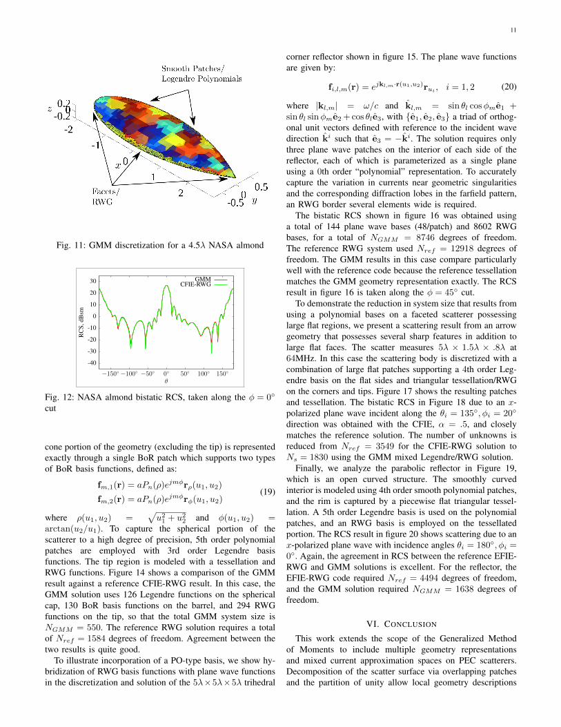
The next scattering result demonstrates automated geometryand basis function assignment for a 4.5λ× 1.5λ× .4λ NASAalmond, with the corresponding RCS compared against awell-validated CFIE-RWG reference solution. The almond isilluminated by a unit amplitude x-polarized plane wave offrequency 300MHz incident in the +z direction. Here, aLegendre basis (eq. 13) of maximum order p = 3 is defined on2nd order polynomial patches in the smooth regions, which aredetected using Algorithm 2. Figure 11 shows the discretizationof the almond in terms of overlapping smooth and tessellatedpatches. Tessellated patches supporting RWG basis functionsare used to capture regions of high curvature and the geometricsingularity at the tip. One could envisage a tip basis functionthat does not rely on tessellation, but instead captures the tipsingularity exactly. While the design of such a basis is outsidethe scope of this paper, it could be seamlessly integratedinto the GMM framework. Figure 12 shows the bistatic RCSfor the almond, which is taken along the φ = 0 cut. Thenumber of degrees of freedom for the CFIE-RWG solution isNref = 3636 and the GMM result requires NGMM = 1861.

The next result, scattering from a 1.2λ × .4λ × .4λdiffraction-matched conesphere illuminated by a −x polarizedplane wave incident in the z direction, illustrates the highdegree of geometrical accuracy that may be obtained when theanalytical form of the underlying scatterer is known. Figure13 illustrates the GMM discretization for the conesphere. The

11

Fig. 11: GMM discretization for a 4.5λ NASA almond

-40

-30

-20

-10

0

10

20

30

−150 −100 −50 0 50 100 150

RC

S,dB

sm

θ

GMMCFIE-RWG

Fig. 12: NASA almond bistatic RCS, taken along the φ = 0

cut

cone portion of the geometry (excluding the tip) is representedexactly through a single BoR patch which supports two typesof BoR basis functions, defined as:

fm,1(r) = aPn(ρ)ejmφrρ(u1, u2)

fm,2(r) = aPn(ρ)ejmφrφ(u1, u2)(19)

where ρ(u1, u2) =√u2

1 + u22 and φ(u1, u2) =

arctan(u2/u1). To capture the spherical portion of thescatterer to a high degree of precision, 5th order polynomialpatches are employed with 3rd order Legendre basisfunctions. The tip region is modeled with a tessellation andRWG functions. Figure 14 shows a comparison of the GMMresult against a reference CFIE-RWG result. In this case, theGMM solution uses 126 Legendre functions on the sphericalcap, 130 BoR basis functions on the barrel, and 294 RWGfunctions on the tip, so that the total GMM system size isNGMM = 550. The reference RWG solution requires a totalof Nref = 1584 degrees of freedom. Agreement between thetwo results is quite good.

To illustrate incorporation of a PO-type basis, we show hy-bridization of RWG basis functions with plane wave functionsin the discretization and solution of the 5λ×5λ×5λ trihedral

corner reflector shown in figure 15. The plane wave functionsare given by:

fi,l,m(r) = ejkl,m·r(u1,u2)rui, i = 1, 2 (20)

where |kl,m| = ω/c and kl,m = sin θl cosφme1 +sin θl sinφme2 + cos θle3, with e1, e2, e3 a triad of orthog-onal unit vectors defined with reference to the incident wavedirection ki such that e3 = −ki. The solution requires onlythree plane wave patches on the interior of each side of thereflector, each of which is parameterized as a single planeusing a 0th order “polynomial” representation. To accuratelycapture the variation in currents near geometric singularitiesand the corresponding diffraction lobes in the farfield pattern,an RWG border several elements wide is required.

The bistatic RCS shown in figure 16 was obtained usinga total of 144 plane wave bases (48/patch) and 8602 RWGbases, for a total of NGMM = 8746 degrees of freedom.The reference RWG system used Nref = 12918 degrees offreedom. The GMM results in this case compare particularlywell with the reference code because the reference tessellationmatches the GMM geometry representation exactly. The RCSresult in figure 16 is taken along the φ = 45 cut.

To demonstrate the reduction in system size that results fromusing a polynomial bases on a faceted scatterer possessinglarge flat regions, we present a scattering result from an arrowgeometry that possesses several sharp features in addition tolarge flat faces. The scatter measures 5λ × 1.5λ × .8λ at64MHz. In this case the scattering body is discretized with acombination of large flat patches supporting a 4th order Leg-endre basis on the flat sides and triangular tessellation/RWGon the corners and tips. Figure 17 shows the resulting patchesand tessellation. The bistatic RCS in Figure 18 due to an x-polarized plane wave incident along the θi = 135, φi = 20

direction was obtained with the CFIE, α = .5, and closelymatches the reference solution. The number of unknowns isreduced from Nref = 3549 for the CFIE-RWG solution toNs = 1830 using the GMM mixed Legendre/RWG solution.

Finally, we analyze the parabolic reflector in Figure 19,which is an open curved structure. The smoothly curvedinterior is modeled using 4th order smooth polynomial patches,and the rim is captured by a piecewise flat triangular tessel-lation. A 5th order Legendre basis is used on the polynomialpatches, and an RWG basis is employed on the tessellatedportion. The RCS result in figure 20 shows scattering due to anx-polarized plane wave with incidence angles θi = 180, φi =0. Again, the agreement in RCS between the reference EFIE-RWG and GMM solutions is excellent. For the reflector, theEFIE-RWG code required Nref = 4494 degrees of freedom,and the GMM solution required NGMM = 1638 degrees offreedom.

VI. CONCLUSION

This work extends the scope of the Generalized Methodof Moments to include multiple geometry representationsand mixed current approximation spaces on PEC scatterers.Decomposition of the scatter surface via overlapping patchesand the partition of unity allow local geometry descriptions

12

capable of handling geometrical features including smoothregions, regions for which a priori functional descriptionis known or can be easily extracted, and regions includinggeometrical singularities. Furthermore, the partition of unitypermits mixtures of multiple classes of Entire Patch and/or SubPatch basis sets within a single simulation. In particular, theintroduction of subpatch basis sets on traditional tessellationsallows straightforward handling of geometrical singularities,even in problems with smooth higher order geometry de-scriptions. Finally, the entire process of geometry and basisassingment can be automated for complex structures. Theresulting method permits discretization the underlying integraloperators in a manner that more closely matches the physicsand may result in significant reductions in the number ofdegrees of freedom required for a given problem relative totraditional moment method solvers.

Although the computational costs associated with assem-bling and solving a GMM system are highly dependent onthe particular mixture of basis sets and patch sizes employed,the cost of the algorithm in both complexity and storage issimilar to that of extant Moment Methods. If currents arepredominantly discretized with entire patch basis functions, thecost scales as that of a mapped higher-order Moment Method;alternatively, if sub-patch basis functions are the principlebasis type, the cost approaches that of traditional tessellation-based schemes such as RWG, rooftop, or GWP bases. The onlyadded cost of evaluating matrix elements in GMM relative totraditional Moment Method schemes is that of computing thepartition of unity, and since the partition of unity on eachpatch is non-unity only in the overlaps between patches, itsevaluation adds very little to the overall complexity.

Future investigations will expand the types of basis func-tions and local geometry parameterizations used in GMM andapply GMM to dielectric problems. One interesting possibilityis to investigate GMM in the context of a domain decompo-sition method (DMM). GMM is a discretization method thatstitches together different basis and geometry descriptions toform a Moment Method system, whereas DDM is a solutionmethod in which the Moment Method system is solved bybreaking the overall problem into subproblems and solvingeach smaller problem individually, subject to global consis-tency constraints. The two methods therefore address differentaspects of the discretization and solution of electromagneticintegral equations, and could possibly complement each otherwell. Using a GMM discretization in a domain decomposi-tion framework would yield a method in which individualsubdomains could be solved independently as in [48] or theEquivalence Principle Algorithm in [49], but where continuoustransitions between non-conformal subdomains are providedby the partition of unity.

Acknowledgements

The authors wish to acknowledge the HPCC facility atMichigan State University and support from NSF CCF-1018516 and NSF CMMI-1250261. D. Dault would liketo acknowledge support from the NSF Graduate ResearchFellowship Program.

REFERENCES

[1] J. Nedelec, “Mixed finite elements in r3,” Numerische Mathematik,vol. 35, pp. 315–341, 1980.

[2] J. Wang and J. Webb, “Hierarchal vector boundary elements and p-adaption for 3-d electromagnetic scattering,” Antennas and Propagation,IEEE Transactions on, vol. 45, no. 12, pp. 1869–1879, 1997.

[3] R. Graglia, D. Wilton, and A. Peterson, “Higher order interpolatoryvector bases for computational electromagnetics,” Antennas and Propa-gation, IEEE Transactions on, vol. 45, pp. 329 –342, mar 1997.

[4] A. Peterson and R. Graglia, “Evaluation of hierarchical vector basisfunctions for quadrilateral cells,” Magnetics, IEEE Transactions on,vol. 47, no. 5, pp. 1190–1193, 2011.

[5] B. Notaros, B. Popovic, J. Weem, R. Brown, and Z. Popovic, “Efficientlarge-domain mom solutions to electrically large practical em problems,”Microwave Theory and Techniques, IEEE Transactions on, vol. 49, no. 1,pp. 151–159, 2001.

[6] E. Jorgensen, J. Volakis, P. Meincke, and O. Breinbjerg, “Higher orderhierarchical legendre basis functions for electromagnetic modeling,”Antennas and Propagation, IEEE Transactions on, vol. 52, no. 11,pp. 2985–2995, 2004.

[7] B. Notaros, “Higher order frequency-domain computational electromag-netics,” Antennas and Propagation, IEEE Transactions on, vol. 56,pp. 2251 –2276, aug. 2008.

[8] L. P. Zha, Y. Q. Hu, and T. Su, “Efficient surface integral equation usinghierarchical vector bases for complex em scattering problems,” Antennasand Propagation, IEEE Transactions on, vol. 60, no. 2, pp. 952–957,2012.

[9] R. Graglia and G. Lombardi, “Singular higher order divergence-conforming bases of additive kind and moments method applicationsto 3d sharp-wedge structures,” Antennas and Propagation, IEEE Trans-actions on, vol. 56, no. 12, pp. 3768–3788, 2008.

[10] M. Djordjevic and B. Notaros, “Double higher order method of momentsfor surface integral equation modeling of metallic and dielectric antennasand scatterers,” Antennas and Propagation, IEEE Transactions on,vol. 52, pp. 2118 – 2129, aug. 2004.

[11] Z.-L. Liu and J. Yang, “Analysis of electromagnetic scattering withhigher-order moment method and nurbs model,” Progress In Electro-magnetics Research, vol. 96, pp. 83–100, 2009.

[12] H. Yuan, N. Wang, and C. Liang, “Combining the higher order methodof moments with geometric modeling by nurbs surfaces,” Antennas andPropagation, IEEE Transactions on, vol. 57, no. 11, pp. 3558–3563,2009.

[13] I. Babuska and J. M. Melenk, “The partition of unity method,” Inter-national Journal for Numerical Methods in Engineering, vol. 40, no. 4,pp. 727–758, 1997.

[14] C. Duarte, I. Babuska, and J. Oden, “Generalized finite element methodsfor three-dimensional structural mechanics problems,” Computers &Structures, vol. 77, no. 2, pp. 215 – 232, 2000.

[15] J. Oden, C. Duarte, and O. Zienkiewicz, “A new cloud-based hpfinite element method,” Computer Methods in Applied Mechanics andEngineering, vol. 153, no. 12, pp. 117 – 126, 1998.

[16] T. Strouboulis, I. Babuska, and K. Copps, “The design and analysis ofthe generalized finite element method,” Computer Methods in AppliedMechanics and Engineering, vol. 181, no. 13, pp. 43 – 69, 2000.

[17] I. Babuska, U. Banerjee, and J. E. Osborn, “Survey of meshless andgeneralized finite element methods: A unified approach,” Acta Numerica,vol. 12, pp. 1–125, 4 2003.

[18] C. Duarte, D.-J. Kim, and D. Quaresma, “Arbitrarily smooth generalizedfinite element approximations,” Computer Methods in Applied Mechan-ics and Engineering, vol. 196, no. 13, pp. 33 – 56, 2006.

[19] E. Perrey-Debain, J. Trevelyan, and P. Bettess, “Plane wave interpolationin direct collocation boundary element method for radiation and wavescattering: numerical aspects and applications,” Journal of Sound andVibration, vol. 261, no. 5, pp. 839 – 858, 2003.

[20] H. Beriot, E. Perrey-Debain, M. B. Tahar, and C. Vayssade, “Plane wavebasis in galerkin bem for bidimensional wave scattering,” EngineeringAnalysis with Boundary Elements, vol. 34, no. 2, pp. 130 – 143, 2010.

[21] M. Peake, J. Trevelyan, and G. Coates, “Novel basis functions for thepartition of unity boundary element method for helmholtz problems,”International Journal for Numerical Methods in Engineering, vol. 93,no. 9, pp. 905–918, 2013.

[22] E. Perrey-Debain, O. Laghrouche, P. Bettess, and J. Trevelyan, “Plane-wave basis finite elements and boundary elements for three-dimensionalwave scattering,” Philosophical Transactions of the Royal Society ofLondon. Series A:Mathematical, Physical and Engineering Sciences,vol. 362, no. 1816, pp. 561–577, 2004.

13

[23] O. Bruno, “Fast, high-order, high-frequency integral methods for com-putational acoustics and electromagnetics,” in Topics in ComputationalWave Propagation (M. Ainsworth, P. Davies, D. Duncan, B. Rynne, andP. Martin, eds.), vol. 31 of Lecture Notes in Computational Science andEngineering, pp. 43–82, Springer Berlin Heidelberg, 2003.

[24] O. P. Bruno and C. A. Geuzaine, “An integration scheme for three-dimensional surface scattering problems,” Journal of Computational andApplied Mathematics, vol. 204, no. 2, pp. 463 – 476, 2007.

[25] T. Belytschko, Y. Krongauz, D. Organ, M. Fleming, and P. Krysl,“Meshless methods: An overview and recent developments,” ComputerMethods in Applied Mechanics and Engineering, vol. 139, no. 14, pp. 3– 47, 1996.

[26] G. Liu, Meshfree Methods: Moving Beyond the Finite Element Method,Second Edition. Taylor & Francis, 2010.

[27] V. Cingoski, N. Miyamoto, and H. Yamashita, “Element-free galerkinmethod for electromagnetic field computations,” Magnetics, IEEE Trans-actions on, vol. 34, no. 5, pp. 3236–3239, 1998.

[28] L. Xuan, Z. Zeng, B. Shanker, and L. Udpa, “Element-free galerkinmethod for static and quasi-static electromagnetic field computation,”Magnetics, IEEE Transactions on, vol. 40, no. 1, pp. 12–20, 2004.

[29] O. Bottauscio, M. Chiampi, and A. Manzin, “Element-free galerkinmethod in eddy-current problems with ferromagnetic media,” Magnetics,IEEE Transactions on, vol. 42, no. 5, pp. 1577–1584, 2006.

[30] C. Lu and B. Shanker, “Hybrid boundary integral-generalized (partitionof unity) finite-element solvers for the scalar helmholtz equation,”Magnetics, IEEE Transactions on, vol. 43, no. 3, pp. 1002–1012, 2007.

[31] O. Tuncer, C. Lu, N. Nair, B. Shanker, and L. Kempel, “Further devel-opment of vector generalized finite element method and its hybridizationwith boundary integrals,” Antennas and Propagation, IEEE Transactionson, vol. 58, no. 3, pp. 887–899, 2010.

[32] W. Nicomedes, R. Mesquita, and F. Moreira, “A local boundary integralequation (lbie) method in 2d electromagnetic wave scattering, and ameshless discretization approach,” in Microwave and OptoelectronicsConference (IMOC), 2009 SBMO/IEEE MTT-S International, pp. 133–137, 2009.

[33] W. Nicomedes, R. Mesquita, and F. Moreira, “A meshless local boundaryintegral equation method for three dimensional scalar problems,” inElectromagnetic Field Computation (CEFC), 2010 14th Biennial IEEEConference on, pp. 1–1, 2010.

[34] M. S. Tong and W. C. Chew, “A novel meshless scheme for solvingsurface integral equations with flat integral domains,” Antennas andPropagation, IEEE Transactions on, vol. 60, no. 7, pp. 3285–3293, 2012.

[35] N. Nair and B. Shanker, “Generalized method of moments: A novel dis-cretization technique for integral equations,” Antennas and Propagation,IEEE Transactions on, vol. 59, pp. 2280 –2293, june 2011.

[36] N. V. Nair and B. Shanker, “Generalized method of moments: a frame-work for analyzing scattering from homogeneous dielectric bodies,” J.Opt. Soc. Am. A, vol. 28, pp. 328–340, Mar 2011.

[37] N. V. Nair, B. Shanker, and L. Kempel, “Generalized method of mo-ments: A boundary integral framework for adaptive analysis of acousticscattering,” The Journal of the Acoustical Society of America, vol. 132,no. 3, pp. 1261–1270, 2012.

[38] N. Nair, B. Shanker, and L. Kempel, “Generalized method of moments:A flexible discretization scheme for integral equations using locallysmooth surface approximations,” in Microwaves, Communications, An-tennas and Electronics Systems (COMCAS), 2011 IEEE InternationalConference on, pp. 1 –4, nov. 2011.

[39] N. Nair, B. Shanker, and L. Kempel, “A discretization framework forscalar integral equations using the generalized method of moments andlocally smooth surface approximations,” in Antennas and Propagation(APSURSI), 2011 IEEE International Symposium on, pp. 3193 –3196,july 2011.

[40] D. Dault, N. Nair, B. Shanker, and L. Kempel, “A flexible framework forthe solution to surface scattering problems using integral equations,” inElectromagnetics in Advanced Applications (ICEAA), 2012 InternationalConference on, pp. 148 –151, sept. 2012.

[41] J. M. Song and W. C. Chew, “Multilevel fast-multipole algorithm forsolving combined field integral equations of electromagnetic scattering,”Microwave and Optical Technology Letters, vol. 10, no. 1, pp. 14–19,1995.

[42] H. Hoppe, T. DeRose, T. Duchamp, J. McDonald, and W. Stuetzle,Surface reconstruction from unorganized points, vol. 26(2). ACM, 1992.

[43] D. Shepard, “A two-dimensional interpolation function for irregularly-spaced data,” in Proceedings of the 1968 23rd ACM national conference,ACM ’68, (New York, NY, USA), pp. 517–524, ACM, 1968.

[44] N. Nair, M. Vikram, and B. Shanker, “Analysis of scattering fromcomplex, electrically large structures using the generalized method of

moments,” in Antennas and Propagation Society International Sympo-sium (APSURSI), 2012 IEEE, pp. 1 –2, july 2012.

[45] A. F. Peterson, “Mapped vector basis functions for electromagnetic inte-gral equations,” Synthesis Lectures on Computational Electromagnetics,vol. 1, no. 1, pp. 1–124, 2006.

[46] J. Song and W. Chew, “Moment method solutions using parametricgeometry,” Journal of Electromagnetic Waves and Applications, vol. 9,no. 1-2, pp. 71–83, 1995.

[47] S. Rao, D. Wilton, and A. Glisson, “Electromagnetic scattering by sur-faces of arbitrary shape,” Antennas and Propagation, IEEE Transactionson, vol. 30, no. 3, pp. 409–418, 1982.

[48] Z. Peng, X.-C. Wang, and J. F. Lee, “Integral equation based domaindecomposition method for solving electromagnetic wave scattering fromnon-penetrable objects,” Antennas and Propagation, IEEE Transactionson, vol. 59, no. 9, pp. 3328–3338, 2011.

[49] M.-K. Li, W. C. Chew, and L. J. Jiang, “A domain decomposition schemebased on equivalence theorem,” Microwave and Optical TechnologyLetters, vol. 48, no. 9, pp. 1853–1857, 2006.

14

Fig. 13: GMM discretization of a 1.2λ× .4λ× .4λ conesphere.

-25

-20

-15

-10

-5

0

5

10

−180−135−90 −45 0 45 90 135 180

RC

S,dB

sm

θ

GMMCFIE-RWG

Fig. 14: Bistatic RCS for conesphere at 300MHz. Wave isincident along the θ = 0, φ = 0 direction with −x-polarization. RCS is taken along φ = 0 cut.

Plane Waves

RWG

Fig. 15: GMM discretization of a 5λ trihedral corner reflector

-40

-30

-20

-10

0

10

20

30

−180−135−90 −45 0 45 90 135 180

RC

S,dB

sm

θ

GMMEFIE-RWG

Fig. 16: Bistatic RCS for trihedral corner reflector at 300MHz.Incident wave is traveling in θi = 45, φi = 45 direction,with x polarization relative to incidence direction. RCS istaken along the φ = 45 cut

(a) (b)

Fig. 17: GMM discretization of a 5λ × 1.5λ × .8λ arrow (a)top view and (b) bottom view

-10

0

10

20

30

40

−180 −135 −90 −45 0 45 90 135 180

RC

S,dB

sm

θ

GMMCFIE-RWG

Fig. 18: Arrow bistatic RCS at 64MHz. Wave is incident inthe θi = 135, φi = 20 direction and is x-polarized relativeto incidence direction. RCS is taken along the φ = 0 cut.

15

(a);

(b)

Fig. 19: GMM discretization for a 4λ × .35λ ParabolicReflector (a) top view and (b) side view

-10

0

10

20

30

40

−180 −135 −90 −45 0 45 90 135 180

RC

S,dB

sm

θ

GMMEFIE-RWG

Fig. 20: Parabolic reflector bistatic RCS. Wave is incident inthe θi = 180, φi = 0 direction with x-polarization. RCS istaken along the φ = 0 cut.