the fast fourier transform - lomont · the fast fourier transform chris lomont, jan 2010, , updated...

The Fast Fourier Transform

Chris Lomont, Jan 2010, http://www.lomont.org, updated Aug 2011 to include parameterized FFTs.

This note derives the Fast Fourier Transform (FFT) algorithm and presents a small, free, public domain

implementation with decent performance. A secondary goal is to derive and implement a real to

complex FFT usable in most cases where engineers use complex to complex FFTs, which gives double the

performance of the usual complex to complex FFT while retaining all the output information. A final goal

is to show how to use the real to complex FFT as a basis for sound processing tasks such as creating

frequency spectrograms.

This work was necessitated by work on the HypnoCube, www.hypnocube.com, which required a small,

free, public domain, decently performing FFT implementation in C#. Since all the FFT implementations

easily found failed on at least one aspect of this, this implementation was created and is released at the

end of this document. The rest of this note details the real to complex FFT construction and how to

apply this faster, lower resource using FFT for sound processing.

Introduction The Fourier Transform converts signals from a time domain to a frequency domain and is the basis for

many sound analysis and visualization algorithms. It converts a signal into magnitudes and phases of the

various sine and cosine frequencies making up the signal.

For example, take the signal shown in Figure 1 from the formula also shown in Figure 1, and sample it at

the 32 equally spaced points shown.

Taking the Fourier Transform of these 32 real valued points results in 32 complex valued points. As

shown later, these 32 points have a symmetry, so plotting only the magnitudes of the first 16 gives the

result in Figure 2; the other 16 points are the mirror image due to the symmetry.

Figure 1:

√

√

Figure 2 - The Fourier Transform of the samples

http://www.lomont.org/

www.hypnocube.com

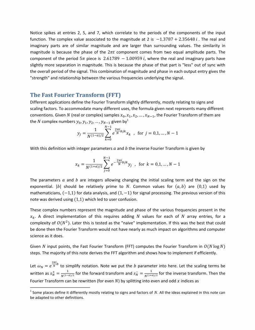
Notice spikes at entries 2, 5, and 7, which correlate to the periods of the components of the input

function. The complex value associated to the magnitude at 2 is . The real and

imaginary parts are of similar magnitude and are larger than surrounding values. The similarity in

magnitude is because the phase of the component comes from two equal amplitude parts. The

component of the period piece is , where the real and imaginary parts have

slightly more separation in magnitude. This is because the phase of that part is "less" out of sync with

the overall period of the signal. This combination of magnitude and phase in each output entry gives the

"strength" and relationship between the various frequencies underlying the signal.

The Fast Fourier Transform (FFT) Different applications define the Fourier Transform slightly differently, mostly relating to signs and

scaling factors. To accommodate many different uses, the formula given next represents many different

conventions. Given (real or complex) samples , the Fourier Transform of them are

the complex numbers given by1

∑

With this definition with integer parameters and the inverse Fourier Transform is given by

∑

The parameters and are integers allowing changing the initial scaling term and the sign on the

exponential. | | should be relatively prime to . Common values for are used by

mathematicians, for data analysis, and for signal processing. The previous version of this

note was derived using which led to user confusion.

These complex numbers represent the magnitude and phase of the various frequencies present in the

. A direct implementation of this requires adding values for each of array entries, for a

complexity of . Later this is tested as the "naive" implementation. If this was the best that could

be done then the Fourier Transform would not have nearly as much impact on algorithms and computer

science as it does.

Given input points, the Fast Fourier Transform (FFT) computes the Fourier Transform in

steps. The majority of this note derives the FFT algorithm and shows how to implement if efficiently.

Let

to simplify notation. Note we put the parameter into here. Let the scaling terms be

written as

for the forward transform and

for the inverse transform. Then the

Fourier Transform can be rewritten (for even ) by splitting into even and odd indices as

1 Some places define it differently mostly relating to signs and factors of . All the ideas explained in this note can

be adapted to other definitions.

∑

∑

⁄

∑

⁄

∑

⁄

∑

⁄

where is the transform of the even indexed data points and

is the transform of the odd

ones2. The value of in front comes from considering the scaling factors and

. If we take

as a power of 2, say , this reducting from to can be repeated until all terms look like

and each is represented by one term, say

, since the Fourier

Transform of a single point is itself.

To see which corresponds with which , expand the case and watch what happens.

To make it clearer we skip writing the scaling factors, but we have to remember them when we

implement. Evaluate , that is, the 5th term

(

)

(

)

((

)

(

))

((

)

(

))

(( )

( ))

(( )

( ))

(( )

( ))

(( )

( ))

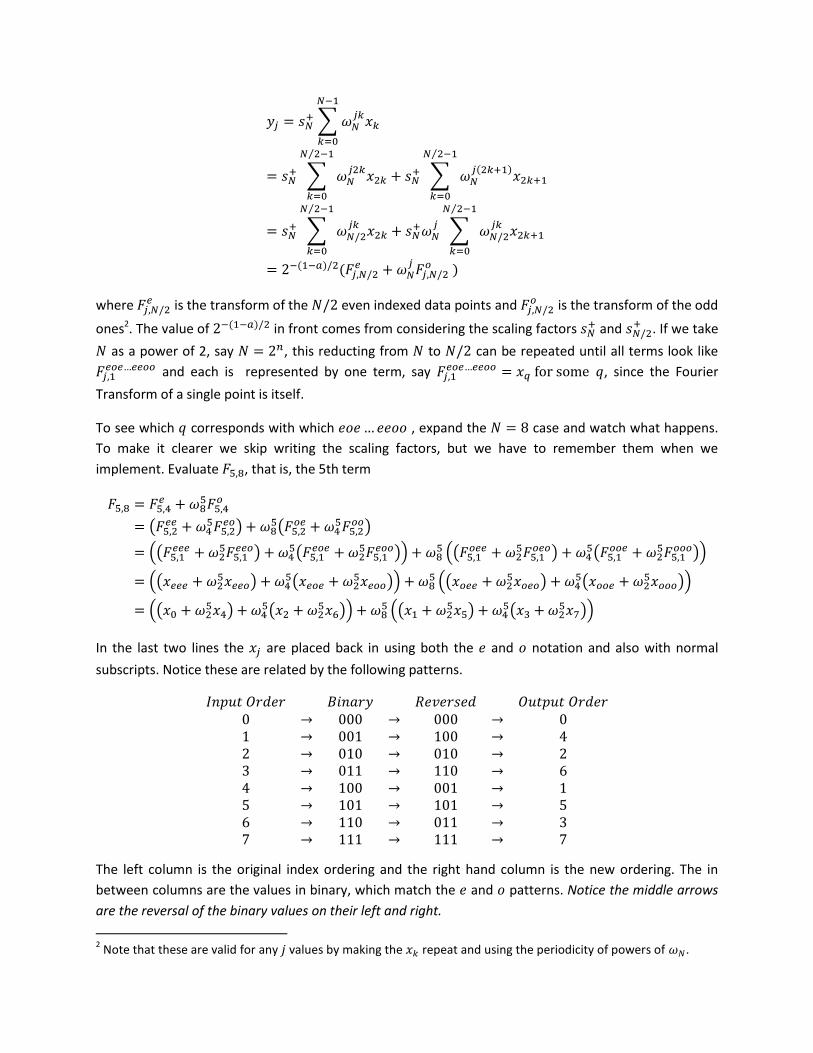
In the last two lines the are placed back in using both the and notation and also with normal

subscripts. Notice these are related by the following patterns.

The left column is the original index ordering and the right hand column is the new ordering. The in

between columns are the values in binary, which match the and patterns. Notice the middle arrows

are the reversal of the binary values on their left and right.

2 Note that these are valid for any values by making the repeat and using the periodicity of powers of .

It appears that the value is obtained by taking the sequence of , replacing and ,

reversing the digits, and using this as the binary value for . Careful analysis shows this pattern holds up

in general.

So, from the last equation, the Fourier Transform can be obtained for by doing a 2-point Fourier

Transform on and , and , and , and and . Then a 4-point can be done on the

results, on indices 0,4,2,6 and 1,5,3,7. Finally these can be merged over all 8 indices in the order

0,4,2,6,1,5,3,7.

Implementing this carefully gives the basic 8 point FFT algorithm consisting of the following steps:

1. Sort the inputs into bit reversed index order, which evaluates the eight transforms.

2. Evaluate four transforms on pairs from step 1.

3. Evaluate two transforms on data from step 2.

4. Evaluate one transform on data from step 3.

The general size transform follows the same pattern, using 1 step of bit reversal (in time

as shown below), and then steps, each using steps to compute for

outcomes. Thus the result is an time algorithm. To do this from the last set of equations

takes careful ordering of how the transforms get done. This algorithm is called the Fast Fourier

Transform, or FFT.

The first step, bit reversing the indices, has an elegant solution. Implementing a bit counter

(0,0,0),(0,0,1),(0,1,0),..., using binary, a carry, and an array to track digits, is straightforward. The trick is

to reverse the array, counting from the left, and create a counter that counts with the digits reversed.

This is then improved to work without arrays by keeping two counters and counting from opposite

directions. Knuth's The Art Of Computer Programming (TAOCP), has a solution in exercise 5, section

7.2.1.1, as follows:

Input: An array of values. Output: The array with item swapped with item if the binary representation of is the reverse of

the binary representation of . Step R1: Initialize Set . Step R2: Swap Swap entries and .

If swap items and and also swap items and . Step R3: Advance k Set . If then stop. Step R4: Advance j Let . while set and . Finally set . Goto step R2.

One final technique is used. In computing the FFT many powers of are used. Instead of computing

them each time one is needed, which requires expensive sine and cosine computations, they can be

computed using a simple recurrence.

Computing the various

can be done by successively multiplying . Using Euler’s expansion

this can be computed using complex multiplication with a recurrence

relation. Using real variables this can be accomplished in steps via:

Input: , an integral power of . Output: The powers of

at various points of the algorithm.

P1: Initialize Set (used as the initial 0th power of ),

and

(the

increment ), and (the current power). P2: Increment Set . Now equals

.

P3: Loop If goto step P2, else end.

There is a slight variant used for increasing numerical robustness. Real numbers are necessarily

represented with finite precision on computers, and for large values of the value of

is very

close to 1. With limited number of digits stored using a binary form of scientific notation, this loses

precision. For example, as the value gets close to 1, say 0.9999, then 0.99999, ... it eventually will round

to 1. It is more precise to store the value

, since in scientific notation more digits will be

retained. This is computed with the trig identity

, avoiding computations that lose

significant digits. Computing

does not suffer this problem since it is already small.

This leads to a slightly more costly to perform algorithm, but one that is numerically better behaved for

large . It uses two more additions per loop than the simpler algorithm, but is still .

Input: , an integral power of . Output: The powers of

at various points of the algorithm.

Q1: Initialize Set (used as the initial 0th power of )

and

, and

(the current power). Q2: Increment Set . Now equals

.

Q3: Loop If goto step P2, else end.

Putting all this together, one obtains a decent FFT algorithm. Careful ordering of indices and the work

gives the following algorithm which transforms the data in place. Assume variables can hold complex

numbers for now, which will be changed later to standard use of real valued variables.

The following algorithm implements this in pseudocode. It works on complex numbers and does the

computation in place, that is, only using a constant amount of extra storage for any value of . The

letter is the complex unit in the code.

Input: DATA, an array of complex numbers . Output: complex values which are the Fourier Transform of the input.

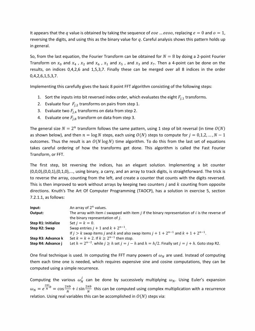
BitReverseData(data) mmax = 1 while (n > mmax) istep = 2 * mmax theta = 3.14159265358979323846 * b / mmax wp = cos(theta) + i * sin(theta) w = 1 for (m = 1; m <= mmax; m = m + 1)

for (k = m - 1; k < n; k = k + istep) j = k + mmax temp = w * x[j] x[j] = x[k] - temp x[k] = x[k] + temp endfor w = w*wp endfor mmax = istep endwhile

ScaleData(data)

This same pseudo code can be used to do the inverse transform by negating theta and changing the

scaling appropriately, allowing merging of FFT and inverse FFT routines into one routine.

Performance Improvements The above algorithm is tested on a modern PC (circa 2010) in several forms and against a few other FFT

implementations. All source code is available for testing on the author's website, www.lomont.org. The

implementations (all tested in C# since that was the driving need for this work) are

1. The "naive" algorithm with running time listed above. This is clearly very slow.

2. The algorithm presented in Numerical Recipes3, a common book of numerical algorithms. Their

license restrictions make this code unusable in almost any application.

3. The NAudio4 library on CodePlex, a C# audio processing library. The FFT routines rely on other

parts of the library, and is much slower then the final real to complex FFT listed below.

4. Lomont1FFT, an implementation of the above algorithm using a lightweight complex number

class. Real valued data is read into the FFT function in an array of alternating real and complex

values, converted to complex numbers, passed through the FFT, and converted back. This is

quite inefficient.

5. Lomont2FFT, which unrolls the complex numbers by replacing each complex entry with two real

entries, but using indices from the above code, resulting in many multiplies by two to access real

components and a multiply by 2 and add one for imaginary components. This is slightly faster.

6. Lomont3FFT, which re-derives the algorithm indices to avoid all the multiplies by two. This and

the next version were the best performing.

7. Lomont4FFT, which pre-computes the sine and cosine values needed and uses them across

multiple runs. This is useful when one does many FFTs of the same size in an application, which

3 http://www.nr.com/

4 http://www.codeplex.com/naudio

http://www.nr.com/

http://www.codeplex.com/naudio

is quite common. This is often the fastest method for doing many applications of the same size

FFT.

This testing does not include FFTW (The "Fastest Fourier Transform in the West"), which is a very high

performance FFT implementation for any size transform. The goal of this work was to create a simple,

single file, small FFT implementation suitable for many projects. FFTW is over 40,000 lines of code. The

result of this work is well under 400 lines of code, including an FFT, an inverse FFT, a table based version

of each, a real to complex FFT (covered below), and its inverse, all in a single standalone source file.

The routines were tested on various sizes of . For each size, the algorithm is run 100 times to load all

items into cache and otherwise smooth out results. Then a loop of 100 applications of the FFT is timed

for 50 passes. The min, max, and average of these 50 scores are kept for each and FFT type

combination. Sizes for were chosen to be small, around those needed in audio processing.

All the following graphs show relative time to Lomont4FFT performance, which was most often the best

performing, with the x-axis being the powers of 2 for the size of the FFT. The values used for the ratios

are the minimum time taken across the runs, which in each case was very near the average run time.

The max run time had noise due to OS interruptions such as thread scheduling, etc. The min time is the

best time the algorithm could do the FFT, which is a pretty good measure of its performance.

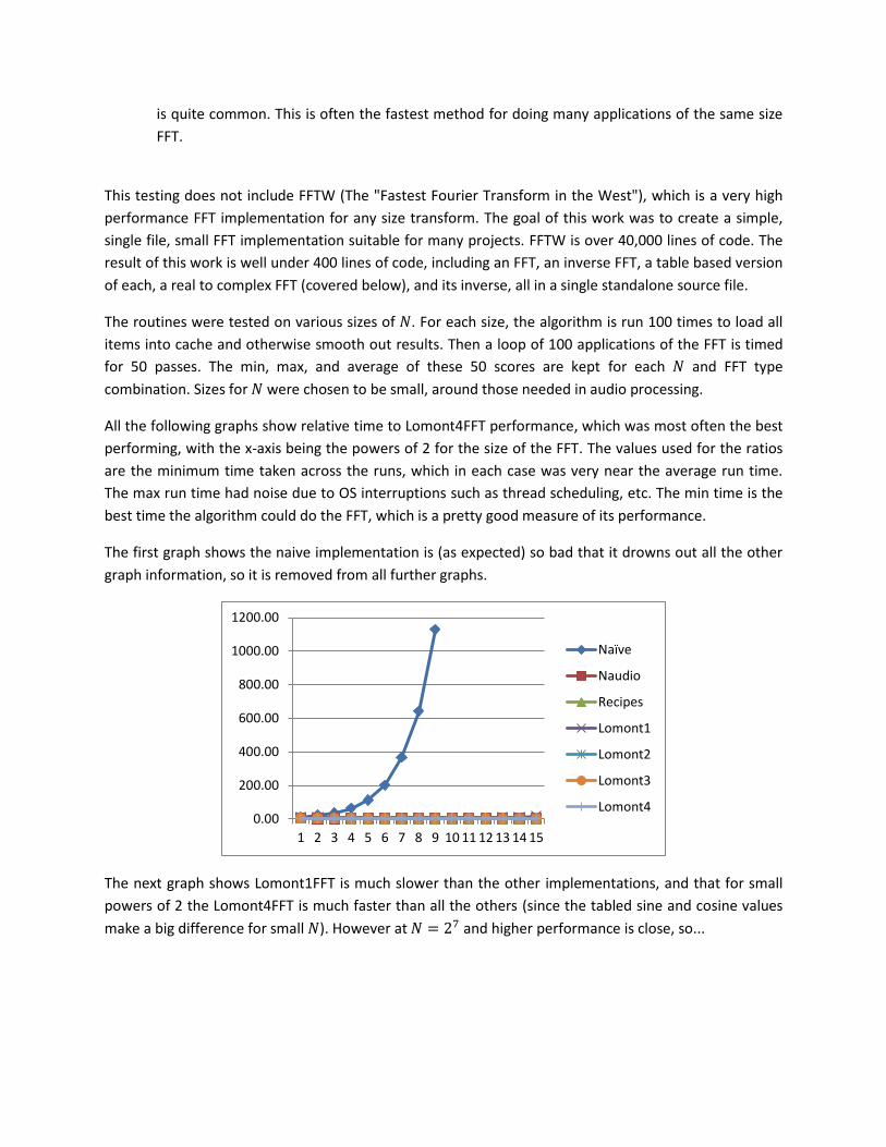
The first graph shows the naive implementation is (as expected) so bad that it drowns out all the other

graph information, so it is removed from all further graphs.

The next graph shows Lomont1FFT is much slower than the other implementations, and that for small

powers of 2 the Lomont4FFT is much faster than all the others (since the tabled sine and cosine values

make a big difference for small ). However at and higher performance is close, so...

0.00

200.00

400.00

600.00

800.00

1000.00

1200.00

1 2 3 4 5 6 7 8 9 10 11 12 13 14 15

Naïve

Naudio

Recipes

Lomont1

Lomont2

Lomont3

Lomont4

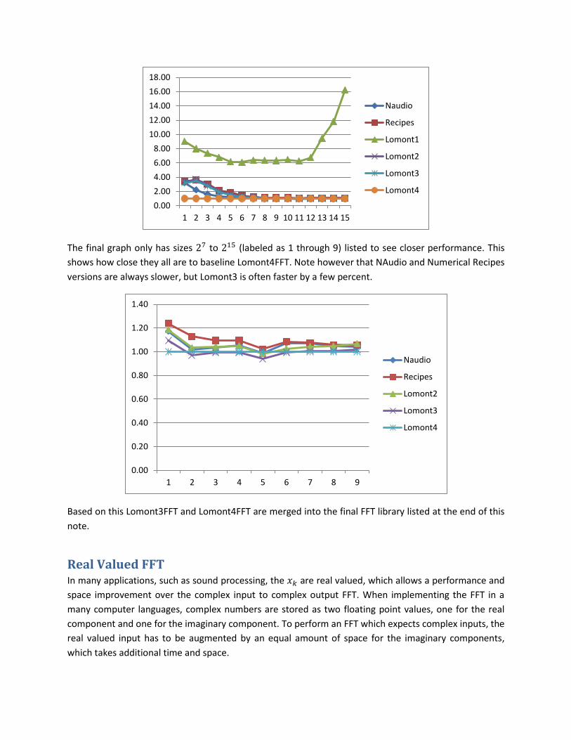
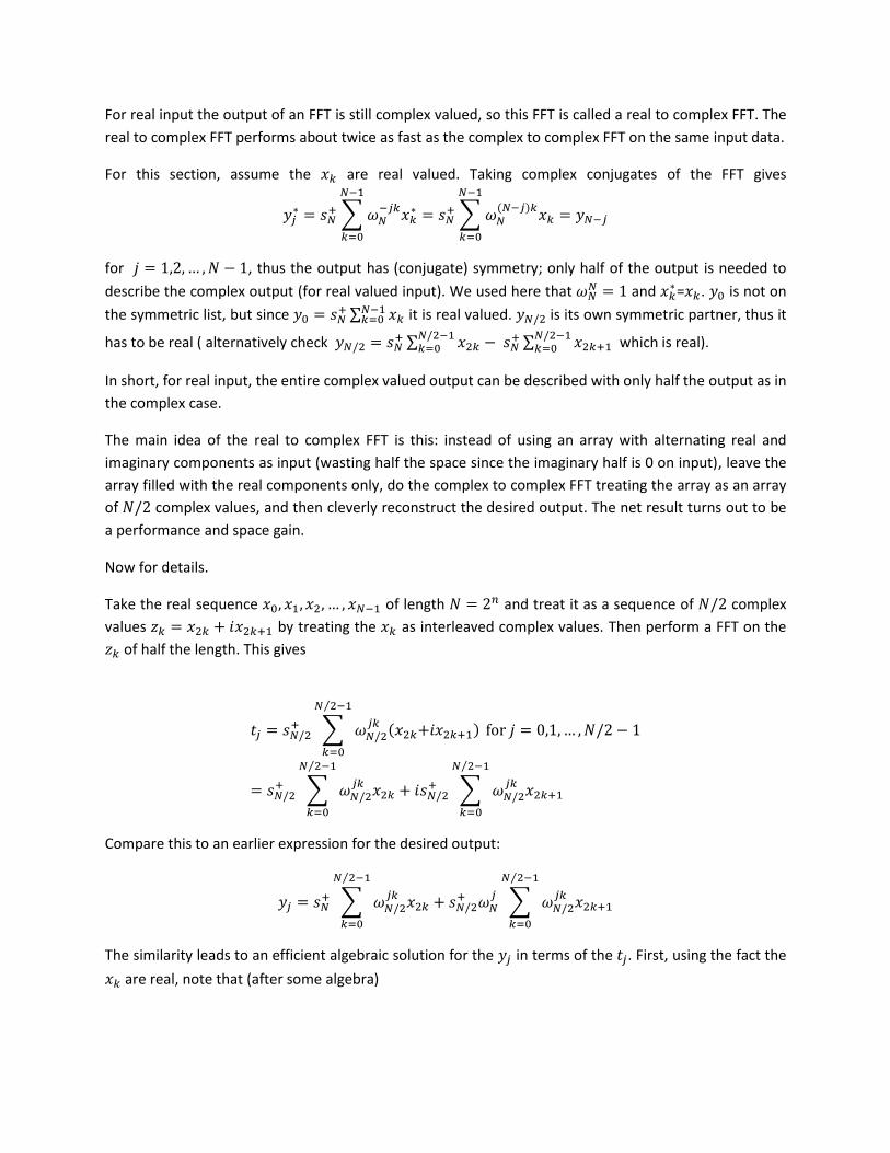
The final graph only has sizes to (labeled as 1 through 9) listed to see closer performance. This

shows how close they all are to baseline Lomont4FFT. Note however that NAudio and Numerical Recipes

versions are always slower, but Lomont3 is often faster by a few percent.

Based on this Lomont3FFT and Lomont4FFT are merged into the final FFT library listed at the end of this

note.

Real Valued FFT In many applications, such as sound processing, the are real valued, which allows a performance and

space improvement over the complex input to complex output FFT. When implementing the FFT in a

many computer languages, complex numbers are stored as two floating point values, one for the real

component and one for the imaginary component. To perform an FFT which expects complex inputs, the

real valued input has to be augmented by an equal amount of space for the imaginary components,

which takes additional time and space.

0.00

2.00

4.00

6.00

8.00

10.00

12.00

14.00

16.00

18.00

1 2 3 4 5 6 7 8 9 10 11 12 13 14 15

Naudio

Recipes

Lomont1

Lomont2

Lomont3

Lomont4

0.00

0.20

0.40

0.60

0.80

1.00

1.20

1.40

1 2 3 4 5 6 7 8 9

Naudio

Recipes

Lomont2

Lomont3

Lomont4

For real input the output of an FFT is still complex valued, so this FFT is called a real to complex FFT. The

real to complex FFT performs about twice as fast as the complex to complex FFT on the same input data.

For this section, assume the are real valued. Taking complex conjugates of the FFT gives

∑

∑

for , thus the output has (conjugate) symmetry; only half of the output is needed to

describe the complex output (for real valued input). We used here that and

= . is not on

the symmetric list, but since ∑

it is real valued. is its own symmetric partner, thus it

has to be real ( alternatively check ∑

∑ which is real).

In short, for real input, the entire complex valued output can be described with only half the output as in

the complex case.

The main idea of the real to complex FFT is this: instead of using an array with alternating real and

imaginary components as input (wasting half the space since the imaginary half is 0 on input), leave the

array filled with the real components only, do the complex to complex FFT treating the array as an array

of complex values, and then cleverly reconstruct the desired output. The net result turns out to be

a performance and space gain.

Now for details.

Take the real sequence of length and treat it as a sequence of complex

values by treating the as interleaved complex values. Then perform a FFT on the

of half the length. This gives

∑

⁄

∑

⁄

∑

⁄

Compare this to an earlier expression for the desired output:

∑

⁄

∑

⁄

The similarity leads to an efficient algebraic solution for the in terms of the . First, using the fact the

are real, note that (after some algebra)

⁄

∑

⁄

∑

⁄

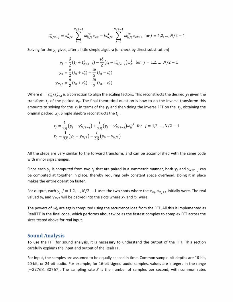
Solving for the gives, after a little simple algebra (or check by direct substitution)

( ⁄

)

( ⁄

)

Where

is a correction to align the scaling factors. This reconstructs the desired given the

transform of the packed . The final theoretical question is how to do the inverse transform: this

amounts to solving for the in terms of the and then doing the inverse FFT on the , obtaining the

original packed . Simple algebra reconstructs the :

( ⁄

)

( ⁄

)

( )

( )

All the steps are very similar to the forward transform, and can be accomplished with the same code

with minor sign changes.

Since each is computed from two that are paired in a symmetric manner, both and can

be computed at together in place, thereby requiring only constant space overhead. Doing it in place

makes the entire operation faster.

For output, each uses the two spots where the initially were. The real

valued and will be packed into the slots where and were.

The powers of

are again computed using the recurrence idea from the FFT. All this is implemented as

RealFFT in the final code, which performs about twice as the fastest complex to complex FFT across the

sizes tested above for real input.

Sound Analysis To use the FFT for sound analysis, it is necessary to understand the output of the FFT. This section

carefully explains the input and output of the RealFFT.

For input, the samples are assumed to be equally spaced in time. Common sample bit-depths are 16-bit,

20-bit, or 24-bit audio. For example, for 16-bit signed audio samples, values are integers in the range

. The sampling rate is the number of samples per second, with common rates

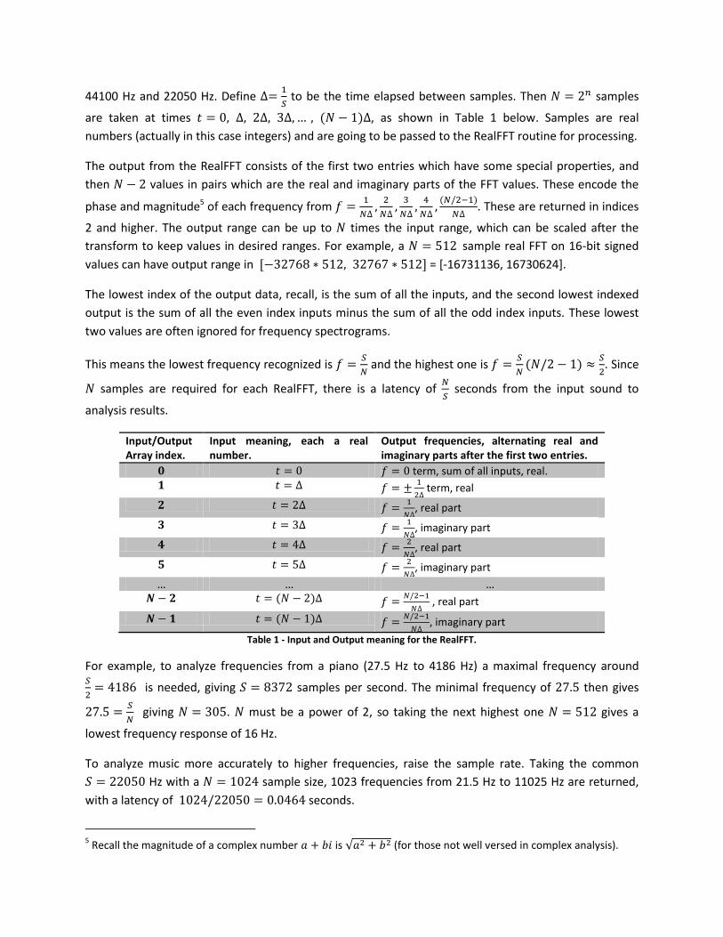
44100 Hz and 22050 Hz. Define

to be the time elapsed between samples. Then samples

are taken at times , as shown in Table 1 below. Samples are real

numbers (actually in this case integers) and are going to be passed to the RealFFT routine for processing.

The output from the RealFFT consists of the first two entries which have some special properties, and

then values in pairs which are the real and imaginary parts of the FFT values. These encode the

phase and magnitude5 of each frequency from

. These are returned in indices

2 and higher. The output range can be up to times the input range, which can be scaled after the

transform to keep values in desired ranges. For example, a sample real FFT on 16-bit signed

values can have output range in = [-16731136, 16730624].

The lowest index of the output data, recall, is the sum of all the inputs, and the second lowest indexed

output is the sum of all the even index inputs minus the sum of all the odd index inputs. These lowest

two values are often ignored for frequency spectrograms.

This means the lowest frequency recognized is

and the highest one is

. Since

samples are required for each RealFFT, there is a latency of

seconds from the input sound to

analysis results.

Input/Output Array index.

Input meaning, each a real number.

Output frequencies, alternating real and imaginary parts after the first two entries.

term, sum of all inputs, real.

term, real

, real part

, imaginary part

, real part

, imaginary part

, real part

, imaginary part

Table 1 - Input and Output meaning for the RealFFT.

For example, to analyze frequencies from a piano (27.5 Hz to 4186 Hz) a maximal frequency around

is needed, giving samples per second. The minimal frequency of then gives

giving . must be a power of 2, so taking the next highest one gives a

lowest frequency response of 16 Hz.

To analyze music more accurately to higher frequencies, raise the sample rate. Taking the common

Hz with a sample size, 1023 frequencies from 21.5 Hz to 11025 Hz are returned,

with a latency of seconds.

5 Recall the magnitude of a complex number is √ (for those not well versed in complex analysis).

The magnitudes of each frequency band give the values needed for a spectrum analyzer. To make larger

bands just aggregate these into the desired number of bands in the desired ranges. This is how to do

basic sound analysis, and code is given next for the various FFTs, one of the most complicated pieces.

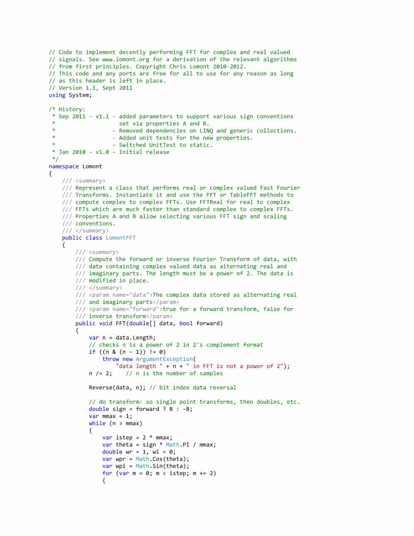
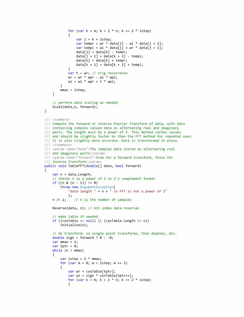
The Code In the code, function FFT implement a standard complex to complex FFT, implementing Lomont3FFT

from testing above. This is the routine to use for a single use complex to complex FFT. The table based

Lomont4FFT algorithm tested above is implemented in TableFFT; it automatically creates the table on

first call, making subsequent calls faster. This is the complex to complex to use for repeated FFTs of the

same size. RealFFT is the real to complex FFT most useful for many needs, such as sound processing. It

uses the TableFFT internally; holding the object between calls is necessary to increase performance.

Each transform takes a data array of doubles and a boolean denoting forward or inverse transforms.

Finally, the FFT routine uses the faster, less accurate recurrence, which is fine for values of

(since an IEEE 754 double has a 53 bit mantissa - another story). This could be replaced with the

recurrence from the Initialize routine to make the FFT more accurate but slightly slower.

The website http://www.lomont.org has a source file for this along with a unit test.

http://www.lomont.org/

// Code to implement decently performing FFT for complex and real valued // signals. See www.lomont.org for a derivation of the relevant algorithms // from first principles. Copyright Chris Lomont 2010-2012. // This code and any ports are free for all to use for any reason as long // as this header is left in place. // Version 1.1, Sept 2011 using System; /* History: * Sep 2011 - v1.1 - added parameters to support various sign conventions * set via properties A and B. * - Removed dependencies on LINQ and generic collections. * - Added unit tests for the new properties. * - Switched UnitTest to static. * Jan 2010 - v1.0 - Initial release */ namespace Lomont { /// <summary> /// Represent a class that performs real or complex valued Fast Fourier /// Transforms. Instantiate it and use the FFT or TableFFT methods to /// compute complex to complex FFTs. Use FFTReal for real to complex /// FFTs which are much faster than standard complex to complex FFTs. /// Properties A and B allow selecting various FFT sign and scaling /// conventions. /// </summary> public class LomontFFT { /// <summary> /// Compute the forward or inverse Fourier Transform of data, with /// data containing complex valued data as alternating real and /// imaginary parts. The length must be a power of 2. The data is /// modified in place. /// </summary> /// <param name="data">The complex data stored as alternating real /// and imaginary parts</param> /// <param name="forward">true for a forward transform, false for /// inverse transform</param> public void FFT(double[] data, bool forward) { var n = data.Length; // checks n is a power of 2 in 2's complement format if ((n & (n - 1)) != 0) throw new ArgumentException( "data length " + n + " in FFT is not a power of 2"); n /= 2; // n is the number of samples Reverse(data, n); // bit index data reversal // do transform: so single point transforms, then doubles, etc. double sign = forward ? B : -B; var mmax = 1; while (n > mmax) { var istep = 2 * mmax; var theta = sign * Math.PI / mmax; double wr = 1, wi = 0; var wpr = Math.Cos(theta); var wpi = Math.Sin(theta); for (var m = 0; m < istep; m += 2) {

for (var k = m; k < 2 * n; k += 2 * istep) { var j = k + istep; var tempr = wr * data[j] - wi * data[j + 1]; var tempi = wi * data[j] + wr * data[j + 1]; data[j] = data[k] - tempr; data[j + 1] = data[k + 1] - tempi; data[k] = data[k] + tempr; data[k + 1] = data[k + 1] + tempi; } var t = wr; // trig recurrence wr = wr * wpr - wi * wpi; wi = wi * wpr + t * wpi; } mmax = istep; } // perform data scaling as needed Scale(data,n, forward); } /// <summary> /// Compute the forward or inverse Fourier Transform of data, with data /// containing complex valued data as alternating real and imaginary /// parts. The length must be a power of 2. This method caches values /// and should be slightly faster on than the FFT method for repeated uses. /// It is also slightly more accurate. Data is transformed in place. /// </summary> /// <param name="data">The complex data stored as alternating real /// and imaginary parts</param> /// <param name="forward">true for a forward transform, false for /// inverse transform</param> public void TableFFT(double[] data, bool forward) { var n = data.Length; // checks n is a power of 2 in 2's complement format if ((n & (n - 1)) != 0) throw new ArgumentException( "data length " + n + " in FFT is not a power of 2" ); n /= 2; // n is the number of samples Reverse(data, n); // bit index data reversal // make table if needed if ((cosTable == null) || (cosTable.Length != n)) Initialize(n); // do transform: so single point transforms, then doubles, etc. double sign = forward ? B : -B; var mmax = 1; var tptr = 0; while (n > mmax) { var istep = 2 * mmax; for (var m = 0; m < istep; m += 2) { var wr = cosTable[tptr]; var wi = sign * sinTable[tptr++]; for (var k = m; k < 2 * n; k += 2 * istep) {

{ var k = n / 2 - j; var tkr = data[2 * k]; // real and imaginary parts of t_k = t_(n/2 - j) var tki = data[2 * k + 1]; var tjr = data[2 * j]; // real and imaginary parts of t_j var tji = data[2 * j + 1]; var a = (tjr - tkr) * wji; var b = (tji + tki) * wjr; var c = (tjr - tkr) * wjr; var d = (tji + tki) * wji; var e = (tjr + tkr); var f = (tji - tki); // compute entry y[j] data[2 * j] = 0.5 * (e + sign * (a + b)); data[2 * j + 1] = 0.5 * (f + sign * (d - c)); // compute entry y[k] data[2 * k] = 0.5 * (e - sign * (b + a)); data[2 * k + 1] = 0.5 * (sign * (d - c) - f); var temp = wjr; // todo - allow more accurate version here? make option? wjr = wjr * wpr - wji * wpi; wji = temp * wpi + wji * wpr; } if (forward) { // compute final y0 and y_{N/2}, store in data[0], data[1] var temp = data[0]; data[0] += data[1]; data[1] = temp - data[1]; } else { var temp = data[0]; // unpack the y0 and y_{N/2}, then invert FFT data[0] = 0.5 * (temp + data[1]); data[1] = 0.5 * (temp - data[1]); // do packed inverse (table based) FFT. This can be changed to // regular inverse FFT to save memory TableFFT(data, false); // scaling - divide by scaling for N, then mult by scaling for N/2 var scale = Math.Pow(2.0, -(A + 1) / 2.0)*2; for (var i = 0; i < data.Length; ++i) data[i] *= scale; } } /// <summary> /// Determine how scaling works on the forward and inverse transforms. /// For size N=2^n transforms, the forward transform gets divided by /// N^((1-a)/2) and the inverse gets divided by N^((1+a)/2). Common /// values for (A,B) are /// ( 0, 1) - default /// (-1, 1) - data processing /// ( 1,-1) - signal processing /// Usual values for A are 1, 0, or -1 /// </summary> public int A { get; set; }

/// <summary> /// Determine how phase works on the forward and inverse transforms. /// For size N=2^n transforms, the forward transform uses an /// exp(B*2*pi/N) term and the inverse uses an exp(-B*2*pi/N) term. /// Common values for (A,B) are /// ( 0, 1) - default /// (-1, 1) - data processing /// ( 1,-1) - signal processing /// Abs(B) should be relatively prime to N. /// Setting B=-1 effectively corresponds to conjugating both input and /// output data. /// Usual values for B are 1 or -1. /// </summary> public int B { get; set; } public LomontFFT() { A = 0; B = 1; } #region Internals /// <summary> /// Scale data using n samples for forward and inverse transforms as needed /// </summary> /// <param name="data"></param> /// <param name="n"></param> /// <param name="forward"></param> void Scale(double[] data, int n, bool forward) { // forward scaling if needed if ((forward) && (A != 1)) { var scale = Math.Pow(n, (A - 1) / 2.0); for (var i = 0; i < data.Length; ++i) data[i] *= scale; } // inverse scaling if needed if ((!forward) && (A != -1)) { var scale = Math.Pow(n, -(A + 1) / 2.0); for (var i = 0; i < data.Length; ++i) data[i] *= scale; } } /// <summary> /// Call this with the size before using the TableFFT version /// Fills in tables for speed. Done automatically in TableFFT /// </summary> /// <param name="size">The size of the FFT in samples</param> void Initialize(int size) { // NOTE: if you port to non garbage collected languages // like C# or Java be sure to free these correctly cosTable = new double[size]; sinTable = new double[size];

// forward pass var n = size; int mmax = 1, pos = 0; while (n > mmax) { var istep = 2 * mmax; var theta = Math.PI / mmax; double wr = 1, wi = 0; var wpi = Math.Sin(theta); // compute in a slightly slower yet more accurate manner var wpr = Math.Sin(theta / 2); wpr = -2 * wpr * wpr; for (var m = 0; m < istep; m += 2) { cosTable[pos] = wr; sinTable[pos++] = wi; var t = wr; wr = wr * wpr - wi * wpi + wr; wi = wi * wpr + t * wpi + wi; } mmax = istep; } } /// <summary> /// Swap data indices whenever index i has binary /// digits reversed from index j, where data is /// two doubles per index. /// </summary> /// <param name="data"></param> /// <param name="n"></param> static void Reverse(double [] data, int n) { // bit reverse the indices. This is exercise 5 in section // 7.2.1.1 of Knuth's TAOCP the idea is a binary counter // in k and one with bits reversed in j int j = 0, k = 0; // Knuth R1: initialize var top = n / 2; // this is Knuth's 2^(n-1) while (true) { // Knuth R2: swap - swap j+1 and k+2^(n-1), 2 entries each var t = data[j + 2]; data[j + 2] = data[k + n]; data[k + n] = t; t = data[j + 3]; data[j + 3] = data[k + n + 1]; data[k + n + 1] = t; if (j > k) { // swap two more // j and k t = data[j]; data[j] = data[k]; data[k] = t; t = data[j + 1]; data[j + 1] = data[k + 1]; data[k + 1] = t; // j + top + 1 and k+top + 1 t = data[j + n + 2]; data[j + n + 2] = data[k + n + 2]; data[k + n + 2] = t; t = data[j + n + 3];

data[j + n + 3] = data[k + n + 3]; data[k + n + 3] = t; } // Knuth R3: advance k k += 4; if (k >= n) break; // Knuth R4: advance j var h = top; while (j >= h) { j -= h; h /= 2; } j += h; } // bit reverse loop } /// <summary> /// Pre-computed sine/cosine tables for speed /// </summary> double [] cosTable; double [] sinTable; #endregion } } // end of file

the fast fourier transform - lomont · the fast fourier transform chris lomont, jan 2010, , updated...

Documents