The Fabry-Perot Interferometer

Exercises:

1. Mounting the beam expander optics on the He–Ne laser and adjustment.

2. Alignment of the total optical setup (laser, interferometer, monochroma-tor).

3. Observing and interpreting all interference patterns produced by the inter-ferometer when performed in parallel and divergent light.

4. Recording the photomultiplier signal corresponding to the interference pat-tern from parallel laser light. Determining the finesse.

5. Aligning a mercury lamp as light source instead of the laser. Recording thehyperfine structure spectrum of the green mercury line at 546.07 nm and ofthe violet one at 404.6 nm. Elaborating these spectra.

Knowledge required:Electromagnetic waves, interference, Fraunhofer diffraction, geometrical optics,atomic spectra.

Bibliography:

The required matter is treated in every textbook of optics, e.g.,

[1] E. Hecht: Optics[2] Optics, by M.V. Klein and T.E. Furtak, Chaps. 3–6;

Optics, by F.G. Smith and J.H. Thomson, Chaps. 6,9,13,14,15[3] R.W. Pohl: Optik und Atomphysik

A profound treatise on the Fabry-Perot interferometer is given in

[4] Spectrophysics, by A. Thorne, U. Litzen and S. Johansson (revisededition of the next book)

[5] Spectrophysics, by A. Thorne, 2nd edition[6] Experiments in Modern Physics, by A.C. Melissinos, Chaps. 7

And a special book is

[7] Fabry-Perot Interferometer, by G. Hernandez

1

Contents

1 Introduction 3

2 Multiple Beam Interference 4

3 The Fabry-Perot Interferometer as a Spectrometer 73.1 General . . . . . . . . . . . . . . . . . . . . . . . . . . . . . . . . 73.2 Halfwidth and free spectral range of the ideal interferometer . . . 83.3 Restrictions and the real interferometer . . . . . . . . . . . . . . . 8

4 Mount of the Interferometer and its Accessories 12

5 Adjustment and Alignment 125.1 Mounting and adjustment of the beam expander . . . . . . . . . . 125.2 Alignment of the laser . . . . . . . . . . . . . . . . . . . . . . . . 155.3 The deflecting mirror M1 . . . . . . . . . . . . . . . . . . . . . . . 155.4 Pumping and gas system . . . . . . . . . . . . . . . . . . . . . . . 165.5 Alignment of the optical elements after the interferometer . . . . . 165.6 Adjusting the interferometer plates . . . . . . . . . . . . . . . . . 18

6 Setting the Instruments 206.1 The monochromator . . . . . . . . . . . . . . . . . . . . . . . . . 206.2 The recorder . . . . . . . . . . . . . . . . . . . . . . . . . . . . . . 216.3 The photomultiplier . . . . . . . . . . . . . . . . . . . . . . . . . . 216.4 Optimizing the signal and test measurement . . . . . . . . . . . . 21

7 Measurements with the He–Ne Laser 227.1 Measuring the Airy function . . . . . . . . . . . . . . . . . . . . . 227.2 Stability of the total experiment . . . . . . . . . . . . . . . . . . . 22

8 Measurements of the Hyperfine Structure of Mercury Lines 228.1 Change of the optical mount . . . . . . . . . . . . . . . . . . . . . 228.2 Measurements with the mercury lamp . . . . . . . . . . . . . . . . 24

9 Evaluation and Analysis 249.1 The finesse . . . . . . . . . . . . . . . . . . . . . . . . . . . . . . . 249.2 The stability . . . . . . . . . . . . . . . . . . . . . . . . . . . . . . 259.3 The refractive index of argon . . . . . . . . . . . . . . . . . . . . . 259.4 Analysis of the hyperfine structure spectra . . . . . . . . . . . . . 25

10 Annex 29

2

1 Introduction

An interferometer is a device to make light beams interfere. A light beam isthe totality of light rays which enter an optical element (lens, mirror, etc.), thearea of which is limited by a diaphragm. The diaphragm may be realized bythe edge of the element itself. According to the difference of phase between thebeams, the interference pattern will have any degree of brightness. When thephase difference locally changes over the cross section of a beam, the interferencepattern is structured and interference fringes can be observed (stripes, rings, andother curves).

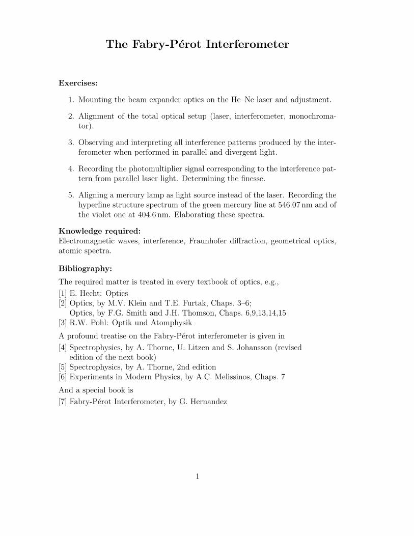
The smallest number of beams to achieve interference is two. The Michelsoninterferometer belongs to the class of two beam interferometers. The light beamscoming from the grooves of a diffraction grating interact to a multiple beaminterference. Here, the number of interfering beams is still limited, though verylarge, 103 . . . 105. In a Fabry-Perot interferometer (Fig. 1), which is anotherdevice to present multiple beam interference, the number of interfering beams isunlimited. It consists of two very plane glass flats in parallel mounting, in whichthe inner faces have a reflection coefficient close to one. The mirrors of a He–Nelaser cavity, which is indeed a Fabry-Perot interferometer, reflect at more than99 %, while in our instrument the coefficient is at 0.94.

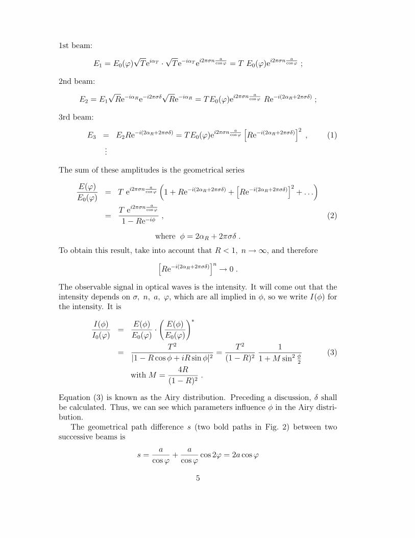
Figure 1: The Fabry-Perot interferometer

Due to the highly reflecting plane surfaces facing each other in parallel mount-ing, an infinite number of parallel beams comes out from the right plate (Fig. 1).They are all superimposed, eventually with a slight lateral displacement in case ofnon-normal incidence of the parallel light on the left plate. The beams distinguishfrom each other by the number of runs between the pair of reflecting planes of theglass plates. When infinitely many waves are superimposed, of course with de-creasing amplitude, constructive interference will be extremely sharp. Therefore,to observe such an interference pattern, the light must be extremely monochro-

3

matic and the reflecting faces extremely plane.This experiment deals with multiple beam interference in a Fabry-Perot in-

terferometer.

2 Multiple Beam Interference

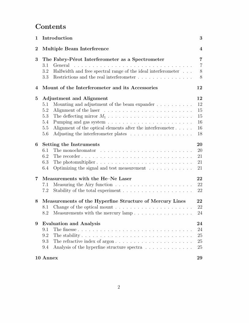
Slightly divergent monochromatic light enters the two glass plates in Fig. 2. Theirfour surfaces are very plane, the inner ones are parallel to each other and highlyreflecting. To guide reflections from the outer faces away, the glass plates arewedged at 0.5. The interference of light from the inner faces is calculated byadding up the amplitudes of all beams leaving the right plate. For the math-ematical treatment we can interpret the divergent beam at the entrance of theplates as a superposition of an infinite number of parallel beams with individualangles of incidence, ϕ, and amplitudes E0(ϕ). The transmission and reflectioncoefficients of the reflecting films on the plates are T and R, respectively, bothrelated to the intensity. There is a phase shift αT after passage through a filmin the order glass – film – medium between the plates. With each reflection at afilm surface, a phase shift of −αR happens when the wave enters the film fromthe side of that medium. In the entity of beams leaving the interferometer at itsright side, two successive beams differ by the bold geometrical path s in Fig. 2,we will call the corresponding optical path difference δ with δ = ns. A few pagesahead, δ will be calculated; δ is a function of the angle of incidence, ϕ. At theexit of the second glass plate, the beams have the following amplitudes, σ = 1/λ(inverse vacuum wavelength):

Figure 2: Multiple beam interference and mutual optical path difference

4

1st beam:

E1 = E0(ϕ)√

T eiαT ·√

T e−iαT ei2πσn acos ϕ = T E0(ϕ)ei2πσn a

cos ϕ ;

2nd beam:

E2 = E1

√Re−iαRe−i2πσδ

√Re−iαR = TE0(ϕ)ei2πσn a

cos ϕ Re−i(2αR+2πσδ) ;

3rd beam:

E3 = E2Re−i(2αR+2πσδ) = TE0(ϕ)ei2πσn acos ϕ

[

Re−i(2αR+2πσδ)]2

, (1)

...

The sum of these amplitudes is the geometrical series

E(ϕ)

E0(ϕ)= T ei2πσn a

cos ϕ

(

1 + Re−i(2αR+2πσδ) +[

Re−i(2αR+2πσδ)]2

+ . . .)

=T ei2πσn a

cos ϕ

1− Re−iφ, (2)

where φ = 2αR + 2πσδ .

To obtain this result, take into account that R < 1, n →∞, and therefore

[

Re−i(2αR+2πσδ)]n → 0 .

The observable signal in optical waves is the intensity. It will come out that theintensity depends on σ, n, a, ϕ, which are all implied in φ, so we write I(φ) forthe intensity. It is

I(φ)

I0(ϕ)=

E(φ)

E0(ϕ)·(

E(φ)

E0(ϕ)

)∗

=T 2

|1−R cos φ + iR sin φ|2 =T 2

(1−R)2

1

1 + M sin2 φ2

(3)

with M =4R

(1−R)2.

Equation (3) is known as the Airy distribution. Preceding a discussion, δ shallbe calculated. Thus, we can see which parameters influence φ in the Airy distri-bution.

The geometrical path difference s (two bold paths in Fig. 2) between twosuccessive beams is

s =a

cos ϕ+

a

cosϕcos 2ϕ = 2a cos ϕ

5

and from thatδ = ns = 2na cos ϕ (4)

and finallyφ

2= αR + 2πnσa cos ϕ . (5)

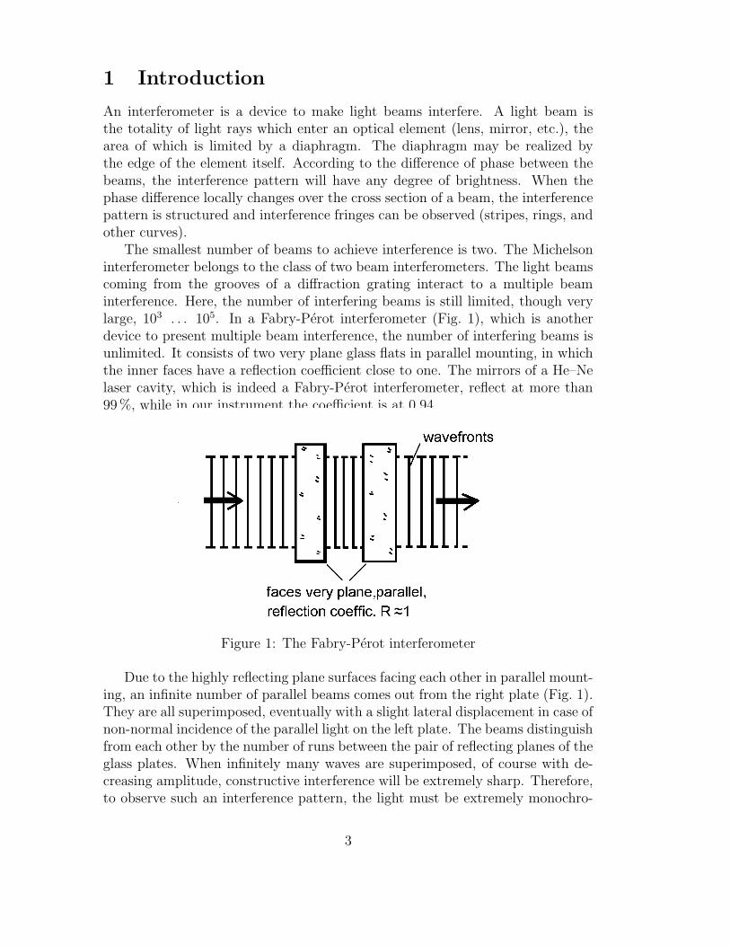
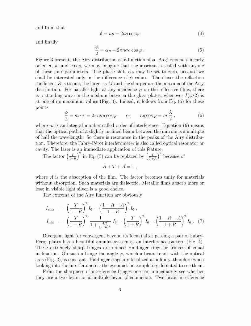
Figure 3 presents the Airy distribution as a function of φ. As φ depends linearlyon n, σ, a, and cosϕ, we may imagine that the abscissa is scaled with anyoneof these four parameters. The phase shift αR may be set to zero, because weshall be interested only in the difference of φ values. The closer the reflectioncoefficient R is to one, the larger is M and the sharper are the maxima of the Airydistribution. For parallel light at any incidence ϕ on the reflective films, thereis a standing wave in the medium between the glass plates, whenever I(φ/2) isat one of its maximum values (Fig. 3). Indeed, it follows from Eq. (5) for thesepoints

φ

2= m · π = 2πnσa cosϕ or na cos ϕ = m

λ

2, (6)

where m is an integral number called order of interference. Equation (6) meansthat the optical path of a slightly inclined beam between the mirrors is a multipleof half the wavelength. So there is resonance in the peaks of the Airy distribu-tion. Therefore, the Fabry-Perot interferometer is also called optical resonator orcavity. The laser is an immediate application of this feature.

The factor(

T1−R

)2in Eq. (3) can be replaced by

(T

T+A

)2because of

R + T + A = 1 ,

where A is the absorption of the film. The factor becomes unity for materialswithout absorption. Such materials are dielectric. Metallic films absorb more orless; in visible light silver is a good choice.

The extrema of the Airy function are obviously

Imax =(

T

1−R

)2

I0 =(

1−R− A

1−R

)2

I0 ,

Imin =(

T

1−R

)2 1

1 + 4R(1−R)2

I0 =(

T

1 + R

)2

I0 =(

1−R− A

1 + R

)2

I0 . (7)

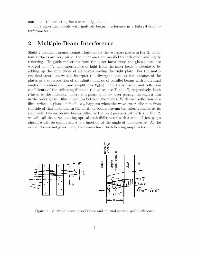
Divergent light (or convergent beyond its focus) after passing a pair of Fabry-Perot plates has a beautiful annulus system as an interference pattern (Fig. 4).These extremely sharp fringes are named Haidinger rings or fringes of equalinclination. On such a fringe the angle ϕ, which a beam tends with the opticalaxis (Fig. 2), is constant. Haidinger rings are localized at infinity, therefore whenlooking into the interferometer, the eye must be completely detented to see them.

From the sharpness of interference fringes one can immediately see whetherthey are a two beam or a multiple beam phenomenon. Two beam interference

6

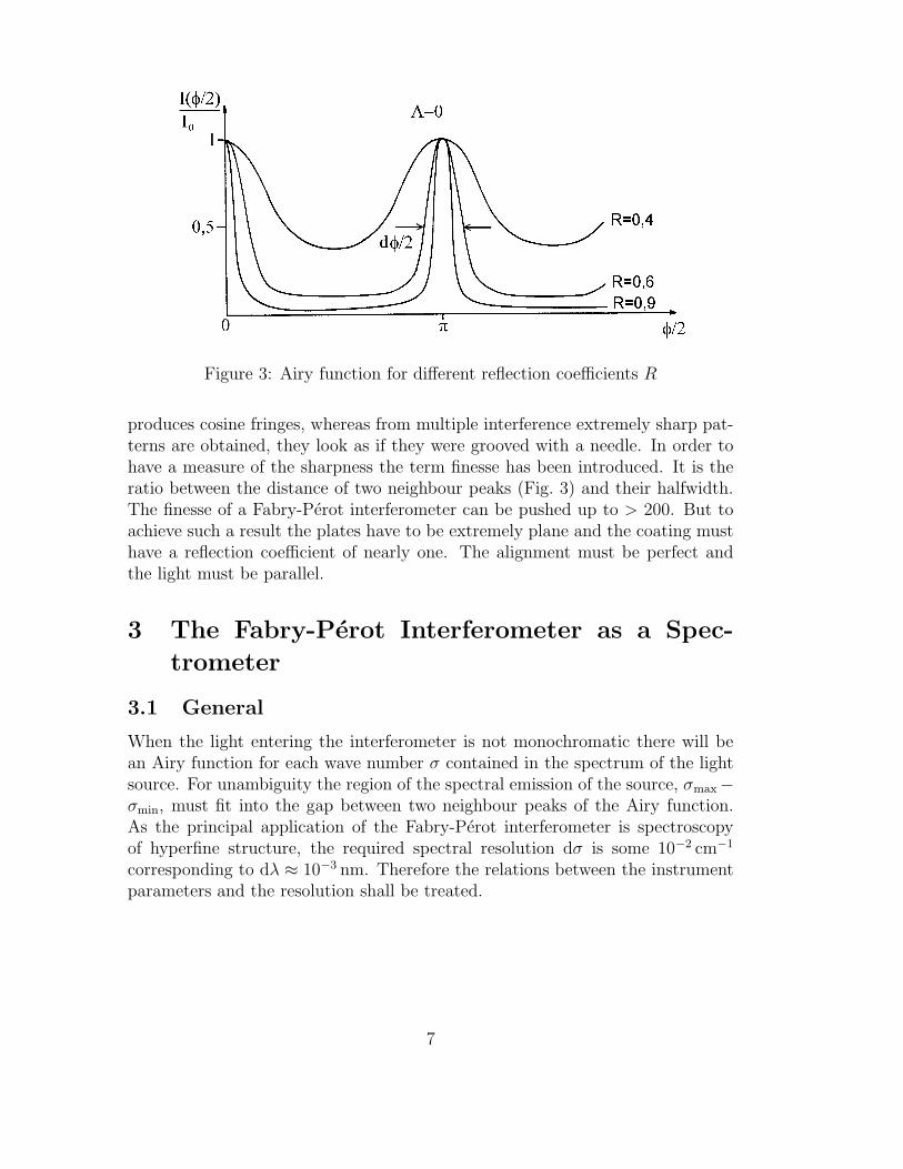
Figure 3: Airy function for different reflection coefficients R

produces cosine fringes, whereas from multiple interference extremely sharp pat-terns are obtained, they look as if they were grooved with a needle. In order tohave a measure of the sharpness the term finesse has been introduced. It is theratio between the distance of two neighbour peaks (Fig. 3) and their halfwidth.The finesse of a Fabry-Perot interferometer can be pushed up to > 200. But toachieve such a result the plates have to be extremely plane and the coating musthave a reflection coefficient of nearly one. The alignment must be perfect andthe light must be parallel.

3 The Fabry-Perot Interferometer as a Spec-

trometer

3.1 General

When the light entering the interferometer is not monochromatic there will bean Airy function for each wave number σ contained in the spectrum of the lightsource. For unambiguity the region of the spectral emission of the source, σmax−σmin, must fit into the gap between two neighbour peaks of the Airy function.As the principal application of the Fabry-Perot interferometer is spectroscopyof hyperfine structure, the required spectral resolution dσ is some 10−2 cm−1

corresponding to dλ ≈ 10−3 nm. Therefore the relations between the instrumentparameters and the resolution shall be treated.

7

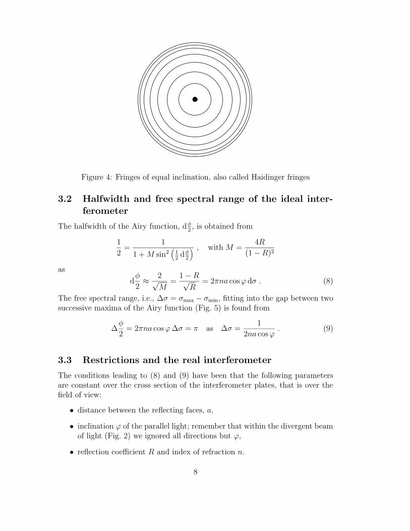
Figure 4: Fringes of equal inclination, also called Haidinger fringes

3.2 Halfwidth and free spectral range of the ideal inter-ferometer

The halfwidth of the Airy function, dφ2, is obtained from

1

2=

1

1 + M sin2(

12dφ

2

) , with M =4R

(1−R)2

as

dφ

2≈ 2√

M=

1−R√R

= 2πna cos ϕ dσ . (8)

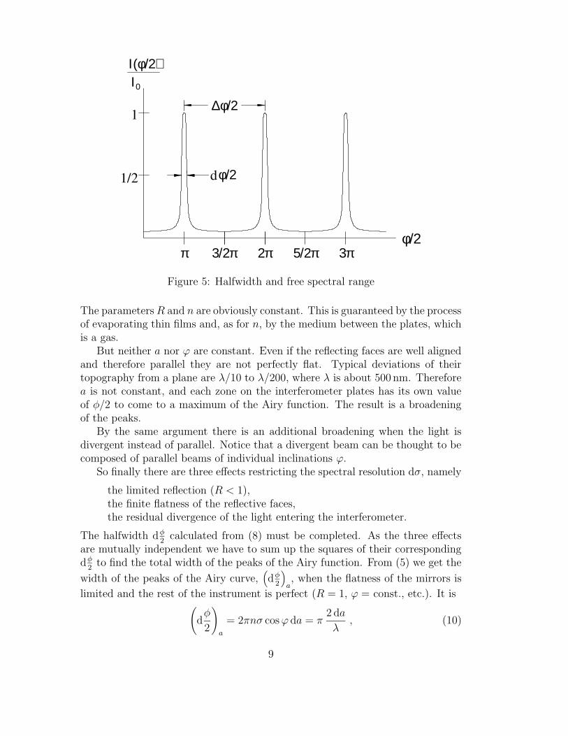
The free spectral range, i.e., ∆σ = σmax − σmin, fitting into the gap between twosuccessive maxima of the Airy function (Fig. 5) is found from

∆φ

2= 2πna cos ϕ ∆σ = π as ∆σ =

1

2na cos ϕ. (9)

3.3 Restrictions and the real interferometer

The conditions leading to (8) and (9) have been that the following parametersare constant over the cross section of the interferometer plates, that is over thefield of view:

• distance between the reflecting faces, a,

• inclination ϕ of the parallel light; remember that within the divergent beamof light (Fig. 2) we ignored all directions but ϕ,

• reflection coefficient R and index of refraction n.

8

φ/23π5/2π2π3/2ππ

1

1/2 φ/2

∆φ/2

d

Ι(φ/2)Ι0

Figure 5: Halfwidth and free spectral range

The parameters R and n are obviously constant. This is guaranteed by the processof evaporating thin films and, as for n, by the medium between the plates, whichis a gas.

But neither a nor ϕ are constant. Even if the reflecting faces are well alignedand therefore parallel they are not perfectly flat. Typical deviations of theirtopography from a plane are λ/10 to λ/200, where λ is about 500 nm. Thereforea is not constant, and each zone on the interferometer plates has its own valueof φ/2 to come to a maximum of the Airy function. The result is a broadeningof the peaks.

By the same argument there is an additional broadening when the light isdivergent instead of parallel. Notice that a divergent beam can be thought to becomposed of parallel beams of individual inclinations ϕ.

So finally there are three effects restricting the spectral resolution dσ, namely

the limited reflection (R < 1),the finite flatness of the reflective faces,the residual divergence of the light entering the interferometer.

The halfwidth dφ2

calculated from (8) must be completed. As the three effectsare mutually independent we have to sum up the squares of their correspondingdφ

2to find the total width of the peaks of the Airy function. From (5) we get the

width of the peaks of the Airy curve,(

dφ2

)

a, when the flatness of the mirrors is

limited and the rest of the instrument is perfect (R = 1, ϕ = const., etc.). It is(

dφ

2

)

a

= 2πnσ cos ϕ da = π2 da

λ, (10)

9

because we can set n ≈ 1 and ϕ ≈ 0. The precision of optical surfaces is alwaysgiven in fractions or multiples of the wavelength. Usually the reference wavelengthis 500 nm. When the deviation from flatness, da, is the µ-th fraction of λ, thenwe obtain (

dφ

2

)

a

= π2

µ. (11)

In the actual interferometer the mirrors have a quality of λ/50. So it is

(

dφ

2

)

a

=π

25. (12)

Again from (5) we obtain the broadening of the peaks(

dφ2

)

ϕwhen the light is

divergent, actually(

dφ

2

)

ϕ

= 2πnaσ d(cos ϕ) , (13)

where −ϕmax < ϕ < +ϕmax and 2ϕmax = ϑ = df.

This time R = 1 and a = const is supposed.

d

f

ϕϑ=2ϕ =m

a xd/f

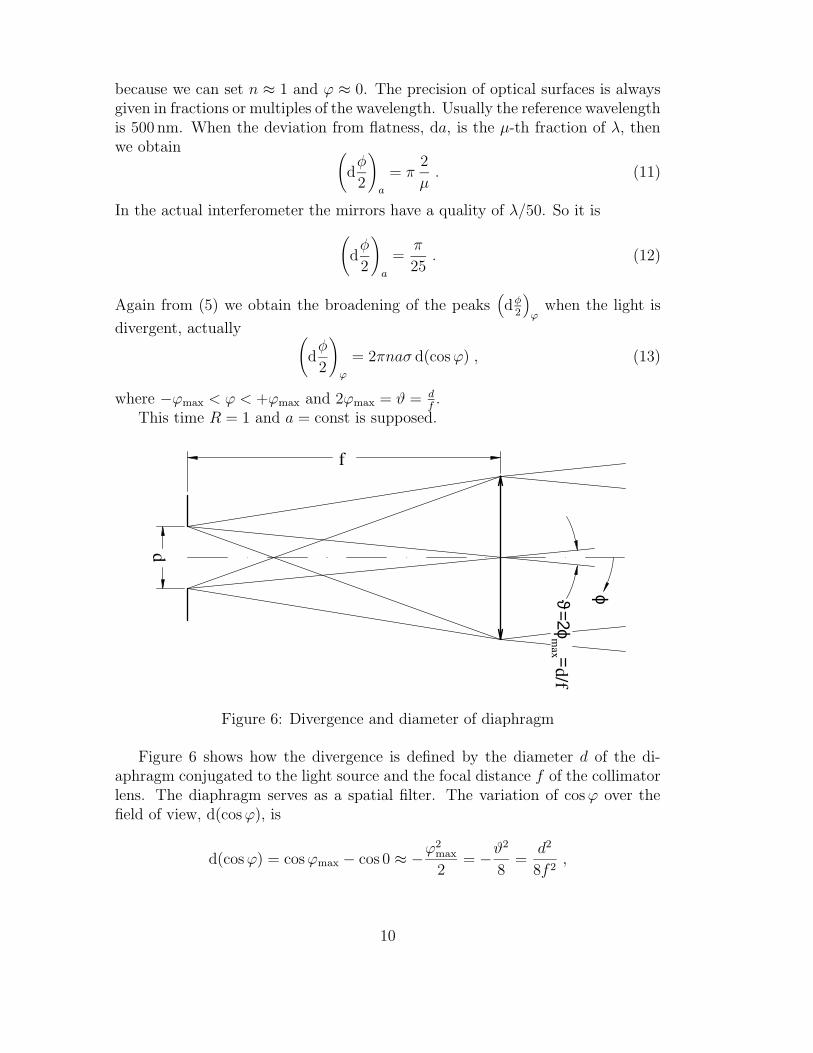
Figure 6: Divergence and diameter of diaphragm

Figure 6 shows how the divergence is defined by the diameter d of the di-aphragm conjugated to the light source and the focal distance f of the collimatorlens. The diaphragm serves as a spatial filter. The variation of cos ϕ over thefield of view, d(cos ϕ), is

d(cos ϕ) = cosϕmax − cos 0 ≈ −ϕ2max

2= −ϑ2

8=

d2

8f 2,

10

and from the preceding equation we obtain(

dφ

2

)

ϕ

= 2πnaσϑ2

8= πnaσ

d2

4f 2. (14)

Calculating the three components of the total dφ2, equipartition of the light in-

tensity over a and ϑ was assumed. This is not necessarily correct. But becausethe real partitions are unknown we stay with this simple assumption.

With each of the three dφ2

just calculated, a finesse of its own is defined,actually

FR =π

(

dφ2

)

R

=π√

R

1−R, Fa =

π(

dφ2

)

a

=µ

2= 25 , Fϕ =

π(

dϕ2

)

ϕ

=4

aσϑ2=

4f 2

aσd2.

(15)The index R signifies the obstriction due to the finite reflection coefficient R. Thetotal finesse, F , measured in the experiment is got from

(

dφ

2

)2

=∑

(

dφ

2

)2

individual

=∑ π2

F 2individual

=π2

F 2(16)

or1

F 2=

1

F 2R

+1

F 2a

+1

F 2ϕ

. (17)

From (16), (8), (11), and (14) the total width of the Airy function is obtained, itis

(

dφ

2

)2

=

(

1− R√R

)2

+4π2

µ2+

π2n2a2σ2d4

16 f 4. (18)

The total width dφ2

limits the spectral resolution, dσ, according to (8):

dσ =dφ

2

2πna cos ϕ≈ dφ

2

2πa; (19)

dφ2

must be taken from (18).Unlike a monochromator, our F.P. interferometer scans the refractive index n

and not σ, which is performed by means of the gas pressure. The peaks generatedby a monochromatic spectral line have a width

dn =dφ

2

2πaσ cos ϕ≈ dφ

2

2πaσ(20)

or, because n− 1 ∼ p,

dp =const · dφ

2

2πaσ cos ϕ≈ const · dφ

2

2πaσ, (21)

again, dφ2

to be taken from (18).

11

An important statement is that at a given pair of F.P. plates (i.e., at fixedflatness and reflection coefficient) and at a fixed entrance diaphragm (d defined bythe required intensity of light), the spectral resolution can be pushed extremelyhigh by increasing the thickness of the etalon, i.e., a. But this is on the dispenseof free spectral range, see (9).

4 Mount of the Interferometer and its Acces-

sories

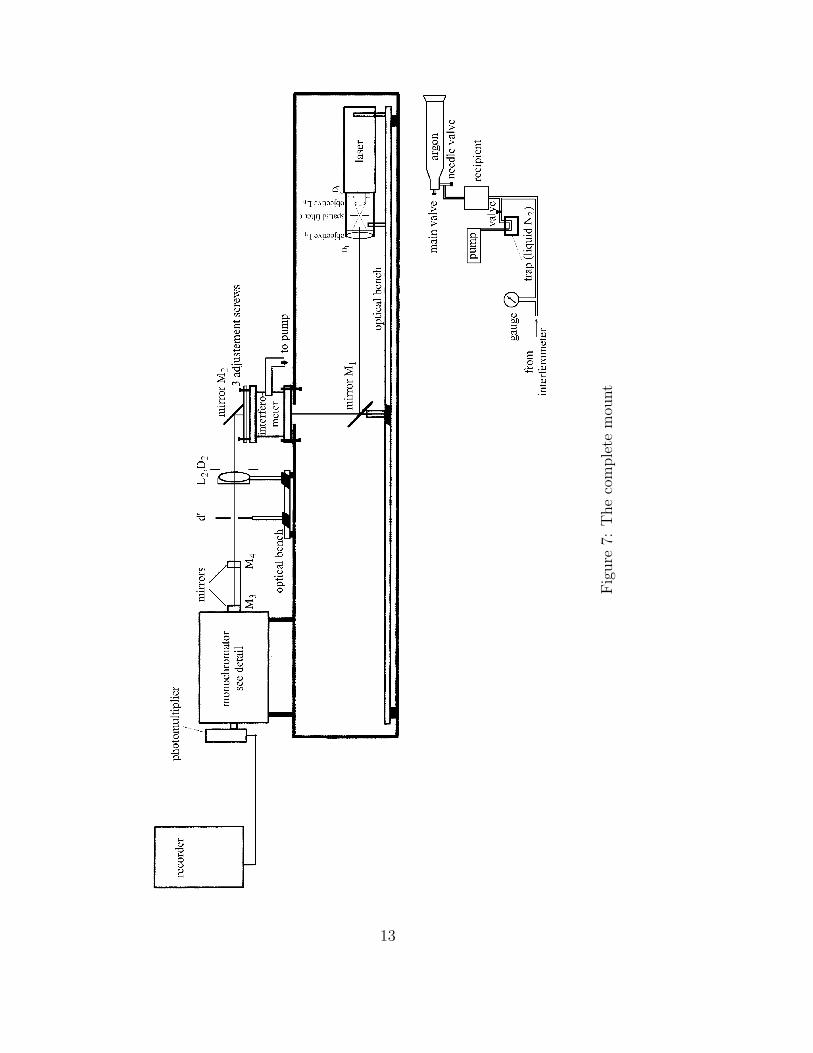
The total mount is shown in Fig. 7. The interferometer is mounted in a littlerecipient which can be evacuated and slowly refilled with argon to scan the phaseφ2

by increasing the refractive index n from 1 to 1.00026. During the scanningthe transmitted light is recorded by a photomultiplier fixed behind the exit slit ofgrating double monochromator. The monochromator (Fig. 8) keeps all spectrallines out apart from the line in question, for example the green mercury line at546.07 nm. Two light sources are on disposition, actually a He–Ne laser and amercury lamp of low pressure.

The laser emits a spectral line which is by far too narrow to be resolved bythe interferometer. The recorded response to such a line is called instrumentfunction, because the spectral light distribution at its entrance is considered asa delta function. Therefore the He–Ne laser is a light source to reveal the finesseand the instrument function of this F.P. interferometer.

The mercury lamp serves as a source to perform a hyperfine structure spec-trum. Good lines for this demonstrations are at 547.07 nm and 404.6 nm, theyare bright and narrow. To avoid Doppler and pressure broadening the dischargeis kept at room temperature and the corresponding saturation pressure.

The laser is equipped with a beam expander and a spatial filter in order toform a beam with very plane wavefronts. The beam expander must be mountedand adjusted on a separate linear bench.

5 Adjustment and Alignment

5.1 Mounting and adjustment of the beam expander

Put the laser on a separate linear bench on the table instead of that one belowit, handling will be easier. Direct the laser beam into the center of the system ofconcentric circles drawn on a white cardboard, which is part of the equipment.Screw the mount of the objective L0 on the laser housing and tighten by meansof the disk on the thread. Adjust L0 until the divergent light beam beyond thefocus is centered on the circles on the cardboard.

12

Fig

ure

7:T

he

com

ple

tem

ount

13

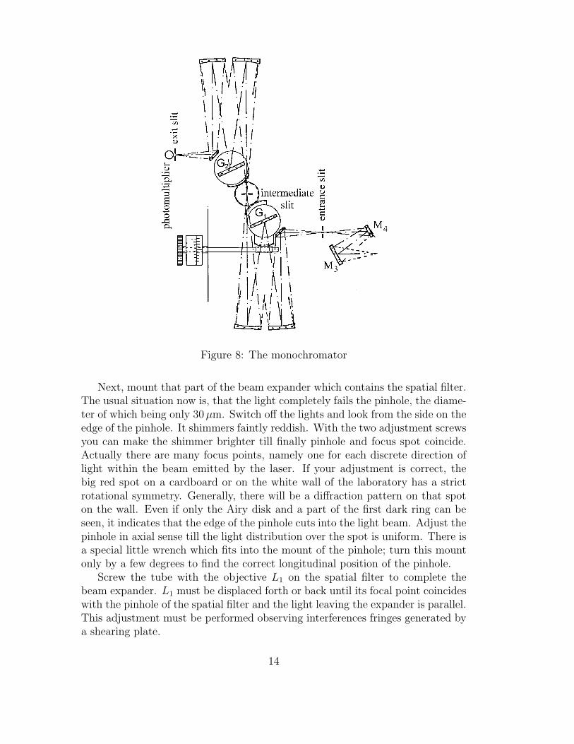
Figure 8: The monochromator

Next, mount that part of the beam expander which contains the spatial filter.The usual situation now is, that the light completely fails the pinhole, the diame-ter of which being only 30 µm. Switch off the lights and look from the side on theedge of the pinhole. It shimmers faintly reddish. With the two adjustment screwsyou can make the shimmer brighter till finally pinhole and focus spot coincide.Actually there are many focus points, namely one for each discrete direction oflight within the beam emitted by the laser. If your adjustment is correct, thebig red spot on a cardboard or on the white wall of the laboratory has a strictrotational symmetry. Generally, there will be a diffraction pattern on that spoton the wall. Even if only the Airy disk and a part of the first dark ring can beseen, it indicates that the edge of the pinhole cuts into the light beam. Adjust thepinhole in axial sense till the light distribution over the spot is uniform. There isa special little wrench which fits into the mount of the pinhole; turn this mountonly by a few degrees to find the correct longitudinal position of the pinhole.

Screw the tube with the objective L1 on the spatial filter to complete thebeam expander. L1 must be displaced forth or back until its focal point coincideswith the pinhole of the spatial filter and the light leaving the expander is parallel.This adjustment must be performed observing interferences fringes generated bya shearing plate.

14

The objective L1 is set correctly and the light is parallel, when the spacingof the interference fringes is at maximum. For details see the annex to theseinstructions.

After these procedures the beam expander is completely adjusted. However,now and then you must check if the spatial filter is still in the correct lateralposition.

5.2 Alignment of the laser

Put the laser on the bench below the table, the cap with the little hole on theexit objective of the expander. From now the thin beam shaped by the little holein the cap will be called ray, when the cap is off we call it beam. Define a markon the cylindrical body of the laser (e.g., label of production) and keep it alwaysin the same azimuthal position. This is necessary because the optical axis of thebeam and the mechanical axis of the cylinder are mutually inclined.

Align the laser ray precisely parallel to the bench at the height of the centerof the mirror which is to deflect the laser light into the interferometer. For thealignment use the special rod clamped in a sliding mount.

rod

in f

a rp o

s itio

n

rod

in n

ear

posi

tion

fron

t mou

nt

rear

mou

nt

Figure 9: Aligning the laser on the optical bench

The rod has a pinhole drilled precisely across its axis. Bring the rod in thenear position to adjust the front mount of the laser, then slide it into the farposition to adjust the rear mount (Fig. 9). Repeat this procedure until the redannulus encircling the pinhole in the rod remains centered in the near and farposition.

5.3 The deflecting mirror M1

Place the sliding mount with the deflecting mirror on the bench at the intersectionwith the axis of the interferometer. Set the inclination of the mirror so that thebrightest among all beams reflected from the interferometer re-enters the hole inthe cap on the laser. Find a position of the sliding mount on the bench to centerthe laser ray on the exit window of the interferometer.

15

For all alignments after the interferometer the transmitted light shall havemaximum brightness. Adjusting the inclination of the deflecting mirror wasfavourized by maximum intensity of the reflected light. Transmitted and re-flected light complete to unity if there is no absorption in the thin films on theF.P. plates. From the shape of the Airy curve it follows that there is strongreflection at nearly every pressure in the interferometer but poor transmission.Therefore, for all further alignments the pressure must be set to obtain maximumtransmission. A short instruction is given how to operate the gas inlet and pump-ing equipment. Respect it seriously because any mistake impairs the quality ofall optical elements inside the interferometer.

5.4 Pumping and gas system

A sketch of the system is comprised in Fig. 7. The pump is filled with oil. Toprotect the optical surfaces from pollution the access to the interferometer etc. isonly through the trap cooled with liquid nitrogen. When the pump is in standbymode, atmospheric air slowly leaks in. Therefore, whenever you open the valvebetween pump and recipient – in the sketch simply called valve – be sure that

• the pump is running

• and the trap is filled with liquid nitrogen.

Close the valve before you switch off the pump.All types of vapour are frozen in the trap, in particular H2O, wherefore thepressure in the interferometer is very constant even when pumping or refilling isstopped at intermediate values between vacuum and atmospheric pressure. Thefinal pressure attained after a few minutes pumping is some 10−2 mbar, althoughthe gauge then indicates about 5 mbar.

When the system is evacuated close valve and pump as described and letargon in. First open the main valve on the big storage bottle while the needlevalve is still closed. There is no reduction valve, which means that the 200 barin the bottle act on the needle valve. It is harmless unless you do stupid things.Slowly open the needle valve while watching the gauge, the needle valve has abacklash of about half a turn. When you close it do not tighten, the thread isvery fine.

5.5 Alignment of the optical elements after the interfer-ometer

a) The principle.The mercury lamp used later in this experiment emits more lines than the greenone at 540.67 nm. These lines must be kept away from the photomultiplier toavoid ambiguity; therefore the monochromator is part of the optical configuration.

16

The parallel beam coming out of the interferometer must be focalized on theentrance slit of the monochromator (Fig. 8) and enter it in a given direction inorder to cover the diffraction grating completely. Fixed with the monochromatorthere is a concave and a plane mirror (M3 and M4, resp.) which form an imageof a light source on the entrance slit with a magnification of unity. M3 and M4

are adjusted that way that the grating G1 is fully illuminated, when an imageof the lamp covers the entrance slit. To keep this adjustment the positions ofM3 and M4 must not be changed. M3 is conjugated to G1 and G2 and musttherefore be symmetrically and fully illuminated. An image of the source mustsymmetrically cover the entrance slit. To achieve the latter, the objective L2 mustform an intermediate image of the spatial filter (pinhole, see beam expander) atthe appropriate distance in front of the concave mirror M3.

b) Alignment of mirror M2

Mirror M2 is mounted on a plate which has three screws for alignment. Theyallow to align the direction of the laser ray in horizontal and vertical sense.However, the adjustments are not mutually independent. Therefore, think aboutthe axis around which the ray will rotate before you turn one of the screws. Inaddition, the vertex of the angle of deflection performed by M2 can be lifted orlowered when turning all screws. The position of the monochromator must notbe changed. For the alignment the following information is helpful: The rayis parallel to the plane of the wooden table when it enters the monochromatorcorrectly.

Put the short bench with the objective L2 aside and align the ray parallel tothe plane of the table, use the special rod. Once the ray is parallel it is easy tomake it hit the center of the concave mirror M3 and the center of the entranceslit.

c) Alignment of the short bench on the tableAlign the short bench by means of the special rod so that bench and laser rayare parallel. The gap between the bench and the interferometer shall be about10 mm.

d) Aligning the objective L2

L2 must be positioned in such a manner that the laser ray is not deflected andthat there is a sharp image of the pinhole inside the beam expander on theentrance slit of the monochromator. The objective is fixed in an eccentric mount.Rotating and lifting the mount, L2 can be aligned. It is useful first to align bymeans of the laser ray, then pull off the cap of the beam expander, correct thealignment, and focus precisely. The correct position of L2 is very close to theinterferometer. You will remark that there is a lot of images in the focal planeof the objective and so in the plane of the slit. Decide for the brightest spot,it is the correct one. Think about the origin of the others, their location andtheir assumed behaviour during scanning. We call these images aberrated andtheir generative beams aberrated beams. They must not be confused with lens

17

aberrations. The concave mirror M3 is inclined with respect to the direction ofthe incident light, so the image on the entrance slit is astigmatic. This means thatM3 forms two separated images of the pinhole on the slit, one behind the other,i.e., a short vertical line, called tangential or meridional image, and another one,which is horizontal and its description is sagittal image. Of course, the tangentialimage guarantees the best separation from the aberrated spots.

e) The pinhole diskThe pinhole disk must be placed on the intermediate image of the pinhole inthe beam expander generated by the lens L2. The little hole in the disk isan additional spatial filter. When you look at the mount of the disk you seeimmediately how it can be aligned.

5.6 Adjusting the interferometer plates

This adjustment shall be done last in order to spend only little time until themeasurement starts. There will be no noticeable change of direction of the beamcoming out of the interferometer, because the correction to be done now is tiny.

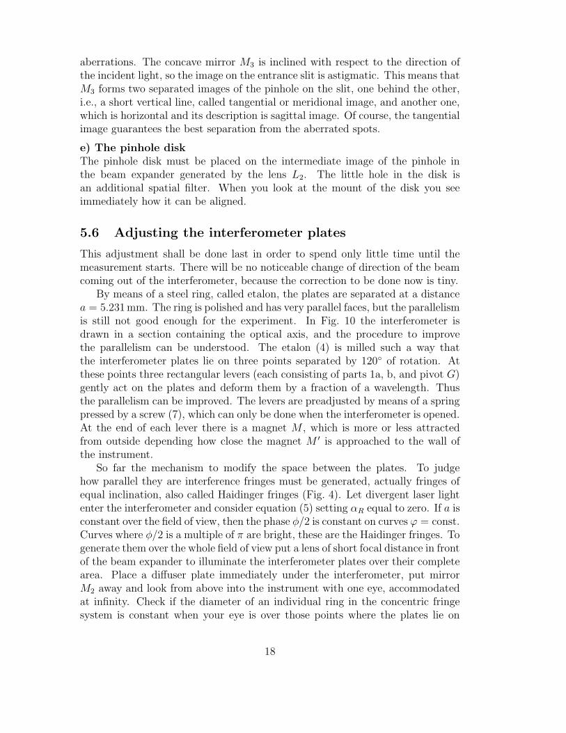
By means of a steel ring, called etalon, the plates are separated at a distancea = 5.231 mm. The ring is polished and has very parallel faces, but the parallelismis still not good enough for the experiment. In Fig. 10 the interferometer isdrawn in a section containing the optical axis, and the procedure to improvethe parallelism can be understood. The etalon (4) is milled such a way thatthe interferometer plates lie on three points separated by 120 of rotation. Atthese points three rectangular levers (each consisting of parts 1a, b, and pivot G)gently act on the plates and deform them by a fraction of a wavelength. Thusthe parallelism can be improved. The levers are preadjusted by means of a springpressed by a screw (7), which can only be done when the interferometer is opened.At the end of each lever there is a magnet M , which is more or less attractedfrom outside depending how close the magnet M ′ is approached to the wall ofthe instrument.

So far the mechanism to modify the space between the plates. To judgehow parallel they are interference fringes must be generated, actually fringes ofequal inclination, also called Haidinger fringes (Fig. 4). Let divergent laser lightenter the interferometer and consider equation (5) setting αR equal to zero. If a isconstant over the field of view, then the phase φ/2 is constant on curves ϕ = const.Curves where φ/2 is a multiple of π are bright, these are the Haidinger fringes. Togenerate them over the whole field of view put a lens of short focal distance in frontof the beam expander to illuminate the interferometer plates over their completearea. Place a diffuser plate immediately under the interferometer, put mirrorM2 away and look from above into the instrument with one eye, accommodatedat infinity. Check if the diameter of an individual ring in the concentric fringesystem is constant when your eye is over those points where the plates lie on

18

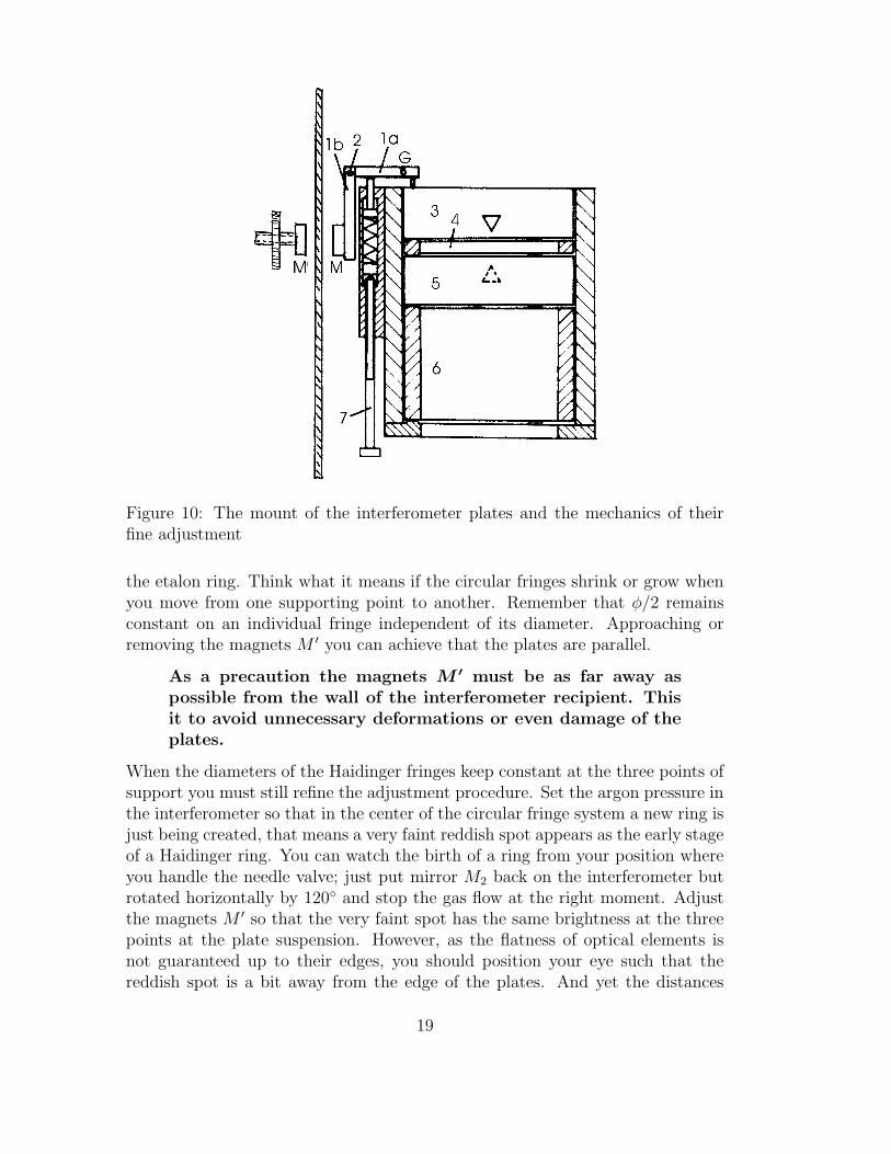
Figure 10: The mount of the interferometer plates and the mechanics of theirfine adjustment

the etalon ring. Think what it means if the circular fringes shrink or grow whenyou move from one supporting point to another. Remember that φ/2 remainsconstant on an individual fringe independent of its diameter. Approaching orremoving the magnets M ′ you can achieve that the plates are parallel.

As a precaution the magnets M′ must be as far away as

possible from the wall of the interferometer recipient. Thisit to avoid unnecessary deformations or even damage of theplates.

When the diameters of the Haidinger fringes keep constant at the three points ofsupport you must still refine the adjustment procedure. Set the argon pressure inthe interferometer so that in the center of the circular fringe system a new ring isjust being created, that means a very faint reddish spot appears as the early stageof a Haidinger ring. You can watch the birth of a ring from your position whereyou handle the needle valve; just put mirror M2 back on the interferometer butrotated horizontally by 120 and stop the gas flow at the right moment. Adjustthe magnets M ′ so that the very faint spot has the same brightness at the threepoints at the plate suspension. However, as the flatness of optical elements isnot guaranteed up to their edges, you should position your eye such that thereddish spot is a bit away from the edge of the plates. And yet the distances

19

should be the same at all three checkpoints, because the brightness of the laserbeam increases radially towards its axis. Use the smallest Haidinger ring to keepa constant gap to the border of the plates (Fig. 11).

Figure 11: Position of Haidinger rings at the three points of support

6 Setting the Instruments

6.1 The monochromator

The monochromator acts as a wavelength filter, as a spatial filter, and as adiaphragm decreasing the brightness on the cathode of the attached photomul-tiplier. Set the gratings at the angle for laser light (632.8 nm) indicated on thebody. Open the entrance slit until the tangential image of the laser spot (a ver-tical line) just disappears between the slit jaws and limit the slit length just likethat; there is a pair of jaws on the slit body to act on the length. Thus theaberrated images are kept away. The true image should not be intersected bythe slit jaws because it could introduce a jitter of the photomultiplier signal. Al-though to total mount (table, optical bench, etc.) is rather stiff, vibrations mayhappen leading to a deflective oscillation of the laser image relative to the slitjaws. The intermediate and the exit slit of the monochromator must be set sothat the image of the entrance slit is fully transmitted. As the magnification ofthe spectrometer is unity you may set the three slits at the same width althoughthis is not the optimum setting.

When the slits are so large the photomultiplier can get too much light. Toprotect it from damage close the diaphragm on lens L2 as far as possible. Youcan open it under control when the photomultiplier and the recorder are switchedon.

20

6.2 The recorder

Apart from plotting the hyperfine structure spectrum and the Airy function therecorder serves as current meter of the photomultiplier current while optimalsettings of all optical elements are being found. The indication of the recorderpin is proportional to the voltage signal at the input and the input impedanceis 1 MΩ at all ranges down to 50 mV. Sensitivity ranges below this figure cannot(and need not) be applied without an interface transforming the anode current ofthe photomultiplier into a voltage signal on a low impedance (I/U amplifier). Asthe signal generated at the recorder input has opposite sign with respect to thevoltage between the last stage and the anode of the photomultiplier the sensitivityrange of the recorder should be a few volts at most to avoid nonlinear feedback.As far the paper transport, set the speed at 20 mm/min to plot the Airy functionand at 1 mm/min when you check the stability of the overall mount.

6.3 The photomultiplier

At last the power supply for the photomultiplier is switched on. Select 550 Vfor the measurements with laser light and 850 V for the hyperfine structure ofthe mercury lines. When you switch on the voltage, you can see from the littleswing of the recorder pin, if the electrical circuitry is alright. To check whetherthe junction between the photomultiplier and the exit slit is tight, increase thesensitivity range of the recorder and switch off the light. There must be no changeof the recorder indication.

6.4 Optimizing the signal and test measurement

Let argon enter extremely slowly and watch the recorder pin (no paper transport).At about 150 mbar there is the first maximum of the Airy function, when laserlight is applied. Stop the gas flow at this pressure, bring the recorder signal atmaximum by refining the settings of the wavelength at the monochromator, ofthe pinhole in the pinhole disk, and of the inclination of mirror M2. By means ofthe diaphragm on lens L2 and of the variable switch on the recorder panel youcan stop the recorder signal at a sufficient height on the scale on the paper. TheAiry function is extremely narrow, the finesse being about 30. If you have failedthe first maximum for this tuning, wait for the next one and stop the gas there.

Make a test run until one or two maxima of the Airy function have passed tosee if everything is as you like it to be. The gas flow must have a rate of about5 mbar/3 sec. Check in the test run if the maximum of the Airy function getsto the same height as before at constant pressure. When the gas streams toofast into the interferometer, the recorder cannot follow and the Airy curve willbe integrated. The time constant of the recorder is about one second. When thetest run was successful fill liquid nitrogen into the trap, if you have not done itbefore, and pump off the argon. Now the measurements can begin.

21

7 Measurements with the He–Ne Laser

7.1 Measuring the Airy function

Make some full runs from p ≈ 0 to atmospheric pressure, each at a differentdiameter of the diaphragm on L2. When you have doubts if the interferometerplates are aligned at best, check it again.

7.2 Stability of the total experiment

You will remark that within the same run the maxima of the Airy function arenot constant. To find the reason stop the gas stream as close as possible at oneof these maxima and plot the photomultiplier signal at constant pressure with1 mm/min paper transport. Wait until you have a plot of about 20 mm andinterpret the signal.

8 Measurements of the Hyperfine Structure of

Mercury Lines

8.1 Change of the optical mount

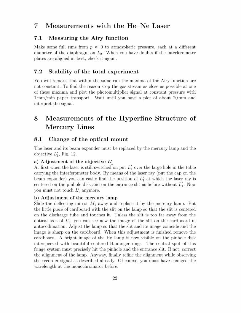
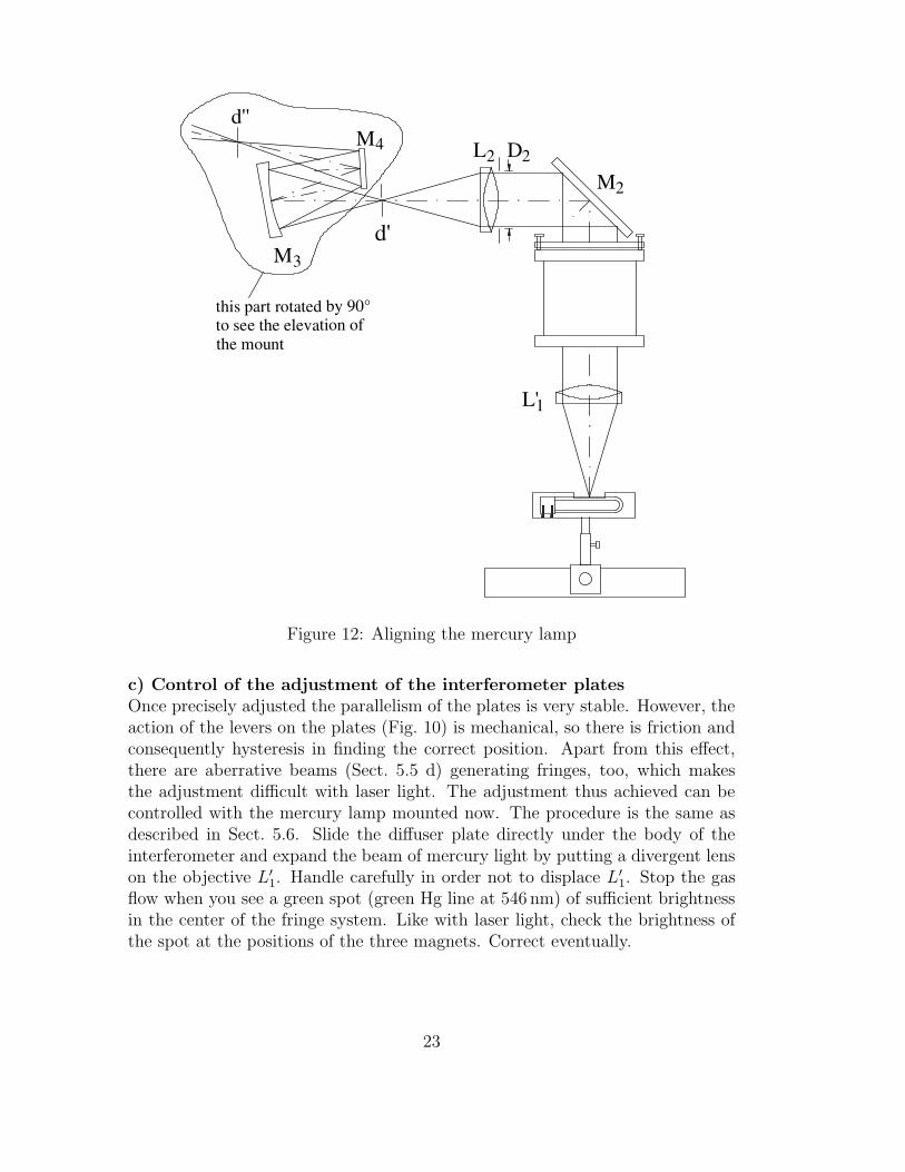
The laser and its beam expander must be replaced by the mercury lamp and theobjective L′

1, Fig. 12.

a) Adjustment of the objective L′

1

At first when the laser is still switched on put L′

1 over the large hole in the tablecarrying the interferometer body. By means of the laser ray (put the cap on thebeam expander) you can easily find the position of L′

1 at which the laser ray iscentered on the pinhole disk and on the entrance slit as before without L′

1. Nowyou must not touch L′

1 anymore.

b) Adjustment of the mercury lampSlide the deflecting mirror M1 away and replace it by the mercury lamp. Putthe little piece of cardboard with the slit on the lamp so that the slit is centeredon the discharge tube and touches it. Unless the slit is too far away from theoptical axis of L′

1, you can see now the image of the slit on the cardboard inautocollimation. Adjust the lamp so that the slit and its image coincide and theimage is sharp on the cardboard. When this adjustment is finished remove thecardboard. A bright image of the Hg lamp is now visible on the pinhole diskinterspersed with beautiful centered Haidinger rings. The central spot of thisfringe system must precisely hit the pinhole and the entrance slit. If not, correctthe alignment of the lamp. Anyway, finally refine the alignment while observingthe recorder signal as described already. Of course, you must have changed thewavelength at the monochromator before.

22

M

L '

M

d '

1

M2

L 24

3

D 2

th is p a r t ro ta te d b y 9 0 ° to s e e th e e le v a tio n o fth e m o u n t

d ''

Figure 12: Aligning the mercury lamp

c) Control of the adjustment of the interferometer platesOnce precisely adjusted the parallelism of the plates is very stable. However, theaction of the levers on the plates (Fig. 10) is mechanical, so there is friction andconsequently hysteresis in finding the correct position. Apart from this effect,there are aberrative beams (Sect. 5.5 d) generating fringes, too, which makesthe adjustment difficult with laser light. The adjustment thus achieved can becontrolled with the mercury lamp mounted now. The procedure is the same asdescribed in Sect. 5.6. Slide the diffuser plate directly under the body of theinterferometer and expand the beam of mercury light by putting a divergent lenson the objective L′

1. Handle carefully in order not to displace L′

1. Stop the gasflow when you see a green spot (green Hg line at 546 nm) of sufficient brightnessin the center of the fringe system. Like with laser light, check the brightness ofthe spot at the positions of the three magnets. Correct eventually.

23

8.2 Measurements with the mercury lamp

a) Tolerable beam divergence and area of the plates for best resolutionMake a run of measurings plotting the photomultiplier signal only for one or twoperiods (interference orders) of spectrum of the green Hg line at 546.07 nm. Keepthe slit widths constant at 1 mm and change each time the size of the pinhole d′

up to 1 mm, the slit width. Look for the best spectral resolution. To comparethe results it is recommended to tune the maxima in the plots at equal heightby means of the variable switch on the recorder panel. The diameter of thepinhole has an impact on the total finesse F in (17), Sect. 3, because it definesthe divergence of the beam generating the interference pattern.

Try also to improve the spectral resolution by decreasing the free area of theinterferometer plates, i.e., reduce the diaphragm D2 on L2. You can combinethe reduction of D2 with the dilation of d′. Depending on the precision of youralignment and also on the partition of flatness over the area of the interferometerplates, a reduction of D2 can improve the corresponding part of the finesse, seeagain (17). Therefore, the still tolerable size of the pinhole may depend upon thediameter D2 and the combination of both changements makes sense.

b) Measuring the hyperfine structure of mercury linesMake at least one full run from p ≈ 0 to atmospheric pressure for the green lineat 546.07 nm and the violet one at 404.6 nm. Check if the maxima are strictlyequidistant and reveal the atmospheric pressure.

9 Evaluation and Analysis

9.1 The finesse

Determine the finesse from your measurements with the laser for different di-aphragms on L2. Is the finesse as could be expected from (15), Sect. 3.2? Com-ment the result! The following list with the parameters of the instrument mightbe useful:

wavelength of He–Ne laser λ = 632.8 nmreflection coefficient of the interferometer plates R = 0.94gap between the plates a = 5.231 mmflatness of the plates λ/50pinhole in the beam expander 30 µmexpansion ratio 25focal distance of objective L1 ≈ 15 cmfocal distance of objective L′

1 30 cmfocal distance of L2 30 cmfocal distance of mirror M3 15 cm

Check if the peaks in the Airy function are rigorously equidistant and commentan eventual deviation.

24

9.2 The stability

List the possible causes to explain the photomultiplier signal plotted in Sect. 7.2.Then note all causes that must be excluded and tell why. You will arrive at theconclusion that the laser itself must be the source of instability. There are twopossibilities to expose such a behaviour, i.e., the intensity and the frequency ofthe laser light. Analyse and comment!

9.3 The refractive index of argon

From the plot with laser light and from that one with the mercury lamp youcan easily determine the refractive index of argon. First make clear that n − 1is proportional to the pressure of argon inside the interferometer. In nearly alltextbooks on optics there is a chapter on dispersive media, theory of dispersion,propagation of light in matter, or something like that. There you find for lowdensity media with n ≈ 1 the dispersion formula n(ω), i.e.,

n2 = (n + 1) · (n− 1) ≈ 2(n− 1) = ω2p

∑

j

fj

ω2j − ω2 + iγjω

(22)

with ω2p =

N2e

mε0

with the following meanings:

ωp plasma frequency of the gas,N density of particles, where N ∼ p because of p = NkT ,e,m charge and mass of an electron,ε0 dielectric constant of vacuum,ω frequency of the light wave,ωj, γj resonance frequencies and corresponding

damping constants of the gas,fj oscillator strengths corresponding to the resonant

frequencies, fj is that part of the N particles whichoscillates at the resonance frequency ωj .

In every maximum of the Airy function the optical path na is a multiple of λ/2.Establish this relation for p ≈ 0 and for atmospheric pressure and subtract onefrom the other to get the refractive index n of argon. For comparison one cantake n from D’Ans-Lax, Physikalische Tabellen, it is

n = 1.00028 at 760 Torr .

9.4 Analysis of the hyperfine structure spectra

According to (6), Sect. 2, the maxima of the Airy function are characterized by

2naσ cos ϕ = m , (23)

25

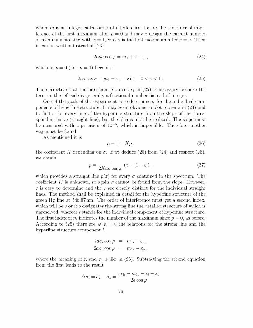
where m is an integer called order of interference. Let m1 be the order of inter-ference of the first maximum after p = 0 and may z design the current numberof maximum starting with z = 1, which is the first maximum after p = 0. Thenit can be written instead of (23)

2naσ cosϕ = m1 + z − 1 , (24)

which at p = 0 (i.e., n = 1) becomes

2aσ cosϕ = m1 − ε , with 0 < ε < 1 . (25)

The corrective ε at the interference order m1 in (25) is necessary because theterm on the left side is generally a fractional number instead of integer.

One of the goals of the experiment is to determine σ for the individual com-ponents of hyperfine structure. It may seem obvious to plot n over z in (24) andto find σ for every line of the hyperfine structure from the slope of the corre-sponding curve (straight line), but the idea cannot be realized. The slope mustbe measured with a precision of 10−5, which is impossible. Therefore anotherway must be found.

As mentioned it isn− 1 = Kp , (26)

the coefficient K depending on σ. If we deduce (25) from (24) and respect (26),we obtain

p =1

2Kaσ cosϕ(z − [1− ε]) , (27)

which provides a straight line p(z) for every σ contained in the spectrum. Thecoefficient K is unknown, so again σ cannot be found from the slope. However,ε is easy to determine and the ε are clearly distinct for the individual straightlines. The method shall be explained in detail for the hyperfine structure of thegreen Hg line at 546.07 nm. The order of interference must get a second index,which will be o or i; o designates the strong line the detailed structure of which isunresolved, whereas i stands for the individual component of hyperfine structure.The first index of m indicates the number of the maximum since p = 0, as before.According to (25) there are at p = 0 the relations for the strong line and thehyperfine structure component i,

2aσi cosϕ = m1i − εi ,

2aσo cosϕ = m1o − εo ,

where the meaning of εi and εo is like in (25). Subtracting the second equationfrom the first leads to the result

∆σi = σi − σo =m1i −m1o − εi + εo

2a cosϕ

26

or, when ∆σ will be replaced by −∆λλ2 ,

∆λi = λi − λo = − λ2

2a cos ϕ

m1i −m1o︸ ︷︷ ︸

∆mi

− (εi − εo)︸ ︷︷ ︸

∆εi

, (28)

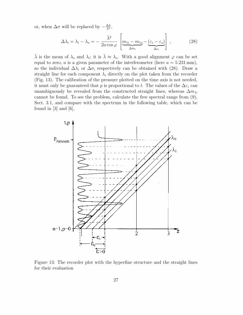
λ is the mean of λo and λi; it is λ ≈ λo. With a good alignment ϕ can be setequal to zero, a is a given parameter of the interferometer (here a = 5.231 mm),so the individual ∆λi or ∆σi respectively can be obtained with (28). Draw astraight line for each component λi directly on the plot taken from the recorder(Fig. 13). The calibration of the pressure plotted on the time axis is not needed,it must only be guaranteed that p is proportional to t. The values of the ∆εi canunambiguously be revealed from the constructed straight lines, whereas ∆m1i

cannot be found. To see the problem, calculate the free spectral range from (9),Sect. 3.1, and compare with the spectrum in the following table, which can befound in [3] and [6],

Figure 13: The recorder plot with the hyperfine structure and the straight linesfor their evaluation

27

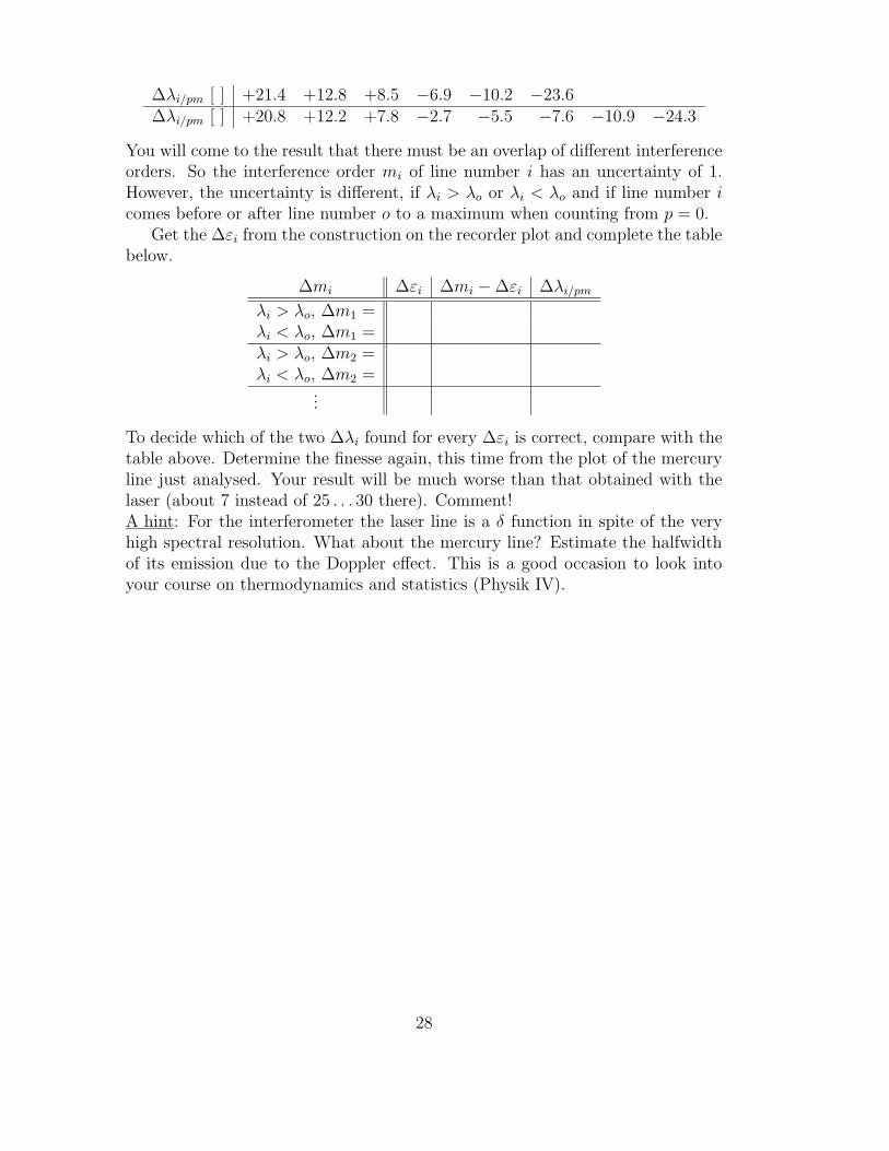
∆λi/pm [ ] +21.4 +12.8 +8.5 −6.9 −10.2 −23.6∆λi/pm [ ] +20.8 +12.2 +7.8 −2.7 −5.5 −7.6 −10.9 −24.3

You will come to the result that there must be an overlap of different interferenceorders. So the interference order mi of line number i has an uncertainty of 1.However, the uncertainty is different, if λi > λo or λi < λo and if line number icomes before or after line number o to a maximum when counting from p = 0.

Get the ∆εi from the construction on the recorder plot and complete the tablebelow.

∆mi ∆εi ∆mi −∆εi ∆λi/pm

λi > λo, ∆m1 =λi < λo, ∆m1 =λi > λo, ∆m2 =λi < λo, ∆m2 =

...

To decide which of the two ∆λi found for every ∆εi is correct, compare with thetable above. Determine the finesse again, this time from the plot of the mercuryline just analysed. Your result will be much worse than that obtained with thelaser (about 7 instead of 25 . . . 30 there). Comment!A hint: For the interferometer the laser line is a δ function in spite of the veryhigh spectral resolution. What about the mercury line? Estimate the halfwidthof its emission due to the Doppler effect. This is a good occasion to look intoyour course on thermodynamics and statistics (Physik IV).

28

10 Annex

Interference by shearing of wavefronts and focalisation of lens L1

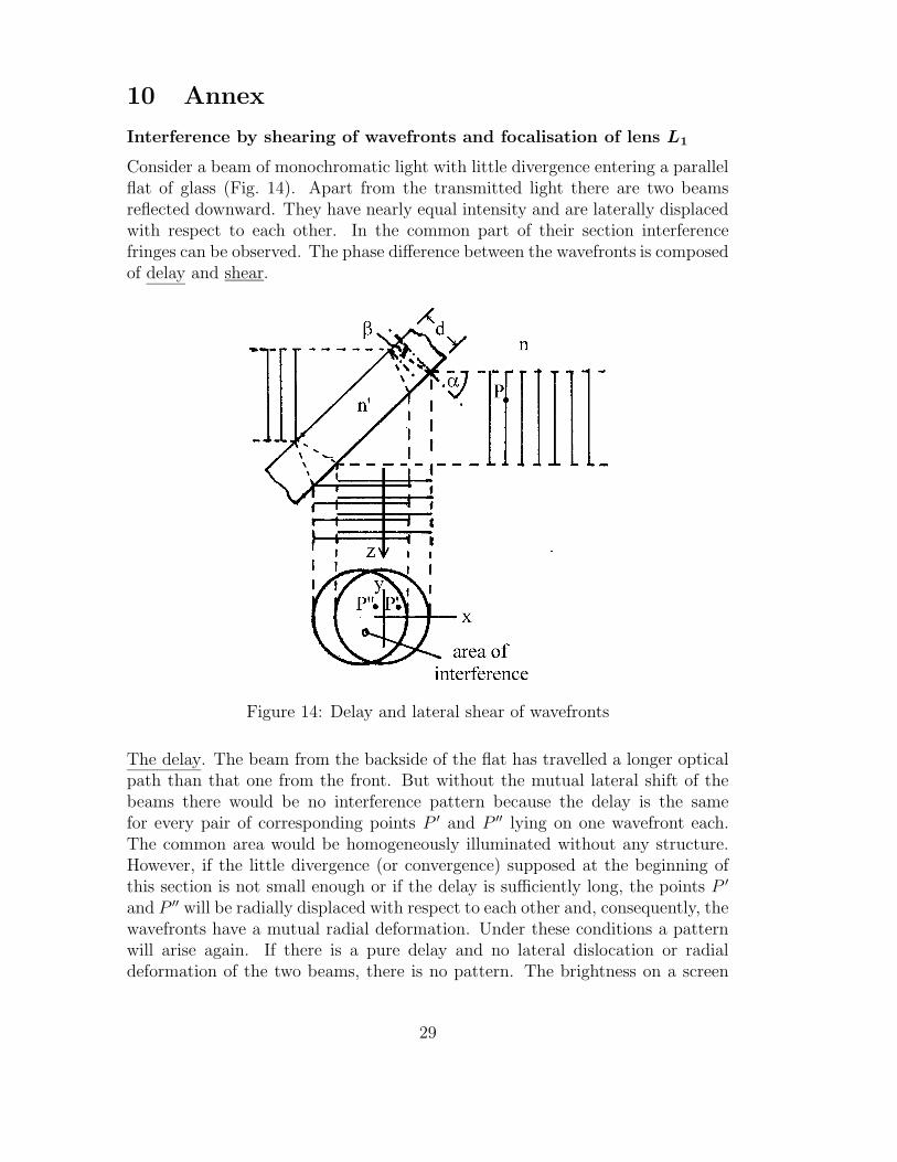
Consider a beam of monochromatic light with little divergence entering a parallelflat of glass (Fig. 14). Apart from the transmitted light there are two beamsreflected downward. They have nearly equal intensity and are laterally displacedwith respect to each other. In the common part of their section interferencefringes can be observed. The phase difference between the wavefronts is composedof delay and shear.

Figure 14: Delay and lateral shear of wavefronts

The delay. The beam from the backside of the flat has travelled a longer opticalpath than that one from the front. But without the mutual lateral shift of thebeams there would be no interference pattern because the delay is the samefor every pair of corresponding points P ′ and P ′′ lying on one wavefront each.The common area would be homogeneously illuminated without any structure.However, if the little divergence (or convergence) supposed at the beginning ofthis section is not small enough or if the delay is sufficiently long, the points P ′

and P ′′ will be radially displaced with respect to each other and, consequently, thewavefronts have a mutual radial deformation. Under these conditions a patternwill arise again. If there is a pure delay and no lateral dislocation or radialdeformation of the two beams, there is no pattern. The brightness on a screen

29

then ranges somewhere between totally dark and fully bright depending on theoptical path difference, that means d, n′, and α.

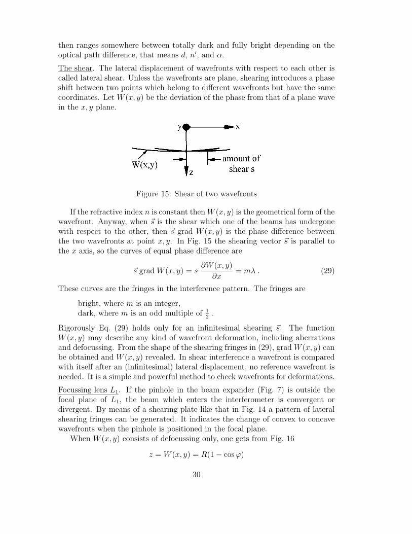
The shear. The lateral displacement of wavefronts with respect to each other iscalled lateral shear. Unless the wavefronts are plane, shearing introduces a phaseshift between two points which belong to different wavefronts but have the samecoordinates. Let W (x, y) be the deviation of the phase from that of a plane wavein the x, y plane.

Figure 15: Shear of two wavefronts

If the refractive index n is constant then W (x, y) is the geometrical form of thewavefront. Anyway, when ~s is the shear which one of the beams has undergonewith respect to the other, then ~s grad W (x, y) is the phase difference betweenthe two wavefronts at point x, y. In Fig. 15 the shearing vector ~s is parallel tothe x axis, so the curves of equal phase difference are

~s grad W (x, y) = s∂W (x, y)

∂x= mλ . (29)

These curves are the fringes in the interference pattern. The fringes are

bright, where m is an integer,dark, where m is an odd multiple of 1

2.

Rigorously Eq. (29) holds only for an infinitesimal shearing ~s. The functionW (x, y) may describe any kind of wavefront deformation, including aberrationsand defocussing. From the shape of the shearing fringes in (29), grad W (x, y) canbe obtained and W (x, y) revealed. In shear interference a wavefront is comparedwith itself after an (infinitesimal) lateral displacement, no reference wavefront isneeded. It is a simple and powerful method to check wavefronts for deformations.

Focussing lens L1. If the pinhole in the beam expander (Fig. 7) is outside thefocal plane of L1, the beam which enters the interferometer is convergent ordivergent. By means of a shearing plate like that in Fig. 14 a pattern of lateralshearing fringes can be generated. It indicates the change of convex to concavewavefronts when the pinhole is positioned in the focal plane.

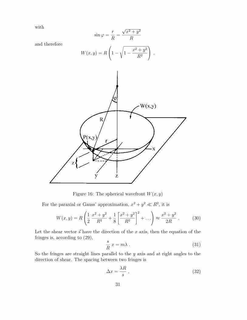
When W (x, y) consists of defocussing only, one gets from Fig. 16

z = W (x, y) = R(1− cos ϕ)

30

with

sin ϕ =r

R=

√x2 + y2

Rand therefore

W (x, y) = R

1−√

1− x2 + y2

R2

.

Figure 16: The spherical wavefront W (x, y)

For the paraxial or Gauss’ approximation, x2 + y2 R2, it is

W (x, y) = R

1

2

x2 + y2

R2+

1

8

[

x2 + y2

R2

]2

+ . . .

≈ x2 + y2

2R. (30)

Let the shear vector ~s have the direction of the x axis, then the equation of thefringes is, according to (29),

s

Rx = mλ . (31)

So the fringes are straight lines parallel to the y axis and at right angles to thedirection of shear. The spacing between two fringes is

∆x =λR

s, (32)

31

infinite spacing indicates parallel light. But when the gap between neighbourfringes exceeds the field of view the control over R is lost. However, when youslightly press against the frame of the shearing plate in order to deform themechanical mount, you can make the neighbour fringes re-enter the field of view,although not simultaneously. But you have nevertheless an estimation whetherthe fringe spacing increases or decreases by your further manipulations with thepinhole position relative to L1.

The shear s can easily be calculated from Fig. 14. It is

s =nd sin 2α√

n′2 − n2 sin2 α. (33)

Inserting s in (31) and (32), one obtains for positioning and spacing of the fringes

nd sin 2α

R√

n′2 − n2 sin2 αx = mλ , (34)

∆x =λR√

n′2 − n2 sin2 α

nd sin 2α. (35)

32