the exponentiated generalized gumbel distribution
TRANSCRIPT
Revista Colombiana de EstadísticaJanuary 2015, Volume 38, Issue 1, pp. 123 to 143DOI: http://dx.doi.org/10.15446/rce.v38n1.48806
The Exponentiated Generalized GumbelDistribution
Distribución Gumbel exponencializada generalizada
Thiago Andrade1,a, Heloisa Rodrigues1,b, Marcelo Bourguignon2,c,Gauss Cordeiro1,d
1Departamento de Estatística, Centro de Ciências Exatas e da Natureza,Universidade Federal de Pernambuco, Recife, Brasil
2Departamento de Estatística, Centro de Ciências da Natureza, UniversidadeFederal do Piauí, Teresina, Brasil
Abstract
A class of univariate distributions called the exponentiated generalizedclass was recently proposed in the literature. A four-parameter model withinthis class named the exponentiated generalized Gumbel distribution is de-fined. We discuss the shapes of its density function and obtain explicit ex-pressions for the ordinary moments, generating and quantile functions, meandeviations, Bonferroni and Lorenz curves and Rényi entropy. The densityfunction of the order statistic is derived. The method of maximum likelihoodis used to estimate model parameters. We determine the observed informa-tion matrix. We provide a Monte Carlo simulation study to evaluate themaximum likelihood estimates of model parameters and two applications toreal data to illustrate the importance of the new model.
Key words: Gumbel Distribution, Maximum Likelihood, Moment, RényiEntropy.
Resumen
Recientemente fue propuesta una clase de distribuciones univariadas cono-cida como la clase exponencializada generalizada. Dentro de esta clase se de-fine un modelo con cuatro parámetros conocido como distribución Gumbelexponencializada generalizada. En este artículo estudiamos las formas de lafunción de densidad de este modelo, obtenemos expresiones explicitas paralos momentos ordinarios, las funciones generadora de momentos y cuantílica,
aGraduate student. E-mail: [email protected] student. E-mail: [email protected] Professor. E-mail: [email protected]. E-mail: [email protected]
123
124 Thiago Andrade, Heloisa Rodrigues, Marcelo Bourguignon & Gauss Cordeiro
para los desvíos medios, las curvas de Bonferroni y Lorenz, y, para la en-tropía de Rényi. Derivamos la función de densidad de la estadística de orden.Usamos el método de máxima verosimilitud para estimar los parámetros delmodelo. Determinamos la matriz de información observada. Presentamosuna simulación de Monte Carlo que evalúa las estimativas de máxima ve-rosimilitud de los parámetros del modelo y presentamos dos aplicaciones adatos reales que ilustran la importancia del modelo nuevo.
Palabras clave: distribución Gumbel, entropía de Rényi, máxima verosi-militud, momentos.
1. Introduction
The Gumbel distribution is a very popular statistical model due to its wideapplicability. An extensive list of the Gumbel model applications can be obtainedin Kotz & Nadarajah (2000). In the area of climate modeling, for example, someapplications of the Gumbel model include: global warming problems, offshoremodeling, rainfall and wind speed modeling (Nadarajah 2006). We can find ap-plications of this model in various areas of engineering such as flood frequencyanalysis, network, nuclear, risk-based, space, software reliability, structural andwind engineering (Cordeiro, Nadarajah & Ortega 2012). Due to its wide appli-cability, several works aimed at extending the Gumbel model become important.Some examples are mentioned in: Nadarajah & Kotz (2004), Nadarajah (2006)and Cordeiro et al. (2012).
The cumulative distribution function (cdf) G(x) and probability density func-tion (pdf) g(x) of the Gumbel (Gu) distribution are given by
G(x;µ, σ) = exp
{−exp
(−x− µ
σ
)}(1)
andg(x;µ, σ) =
1
σexp
{−[x− µσ
+ exp
(−x− µ
σ
)]}, (2)
respectively, for x ∈ R, µ ∈ R and σ > 0.In recent years, some different generalizations of continuous distributions have
received great attention in the literature. Here, we refer to the papers: Marshall& Olkin (1997) for the Marshall-Olkin class, Eugene, Lee & Famoye (2002) forthe Beta class, Zografos & Balakrishnan (2009) and Ristic & Balakrishnan (2011)for the Gamma class and Cordeiro & de Castro (2011) for the Kumaraswamyclass of distributions. In a similar manner, for any baseline cdf G(x), and x ∈ R,Cordeiro, Ortega & Cunha (2013) defined the exponentiated generalized (EG) classof distributions with two extra parameters α > 0 and β > 0 and cdf F (x) and pdff(x) given by
F (x) = {1− [1−G(x)]α}β (3)
andf(x) = αβ[1−G(x)]α−1{1− [1−G(x)]α}β−1g(x), (4)
Revista Colombiana de Estadística 38 (2015) 123–143
The EGGu Distribution 125
respectively. In this paper, we study the so-called exponentiated generalized Gum-bel (“EGGu” for short) distribution by inserting (1) in equation (3).
The rest of the paper is organized as follows. In Section 2, we define the EGGudistribution. Shapes of the density function are discussed in Section 3. Explicitexpressions for cumulative and density functions, quantile function, ordinary mo-ments, mean deviations, Bonferroni and Lorenz curves, generating function, Rényientropy and order statistics are derived in Section 4. We discuss maximum like-lihood estimation and present a Monte Carlo simulation experiment to evaluatethe maximum likelihood estimates (MLEs) of the model parameters in Section 5.Two applications in Section 6 illustrate the usefulness of the new distribution fordata modeling. Lastly, concluding remarks are given in Section 7.
2. The EGGu distribution
The EGGu distribution was proposed by Cordeiro et al. (2013), but they didnot study its mathematical properties. The cdf and pdf of the EGGu distributionare given by
F (x) = F (x;α, β, µ, σ) =
{1−
{1− exp
[− exp
(−x− µ
σ
)]}α}β(5)
and
f(x) = f(x;α, β, µ, σ) =αβ
σexp
{−[x− µσ
+ exp
(−x− µ
σ
)]}{
1− exp
[− exp
(−x− µ
σ
)]}α−1{
1−[1− exp
[− exp
(−x− µ
σ
)]]α}β−1,
(6)
respectively.Henceforth, a random variable X having density function (6) is denoted by
X ∼ EGGu(α, β, µ, σ). We write F (x) = F (x;α, β, µ, σ) in order to eliminatethe dependence on the model parameters. In this model, µ ∈ R and σ > 0 arethe location and scale parameters, respectively, whereas α > 0 and β > 0 arethe shape parameters. The Gumbel distribution is clearly a special case of (5)when α = β = 1. Setting β = 1 we obtain the exponentiated Gumbel distributiondefined by Nadarajah (2006).
3. Shape
The main features of the density shape can be perceived through the studyof its first and second derivative. Regarding the EGGu distribution, the firstderivative of log{f(x)} is
Revista Colombiana de Estadística 38 (2015) 123–143
126 Thiago Andrade, Heloisa Rodrigues, Marcelo Bourguignon & Gauss Cordeiro
d log{f(x)}dx
=1
σ
{−1− ln(z)
[1− (α− 1) z
(1− z)+α (β − 1) z (1− z)α−1
[1− (1− z)α]
]},
where z = exp[− exp
(−x−µσ
)]. Here, 0 < z < 1.
The critical values of f(x) are the roots of the equation:
(α− 1) z
(1− z)− α (β − 1) z (1− z)α−1
[1− (1− z)α]=
ln(z) + 1
ln(z). (7)
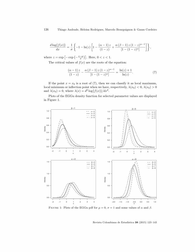
If the point x = x0 is a root of (7), then we can classify it as local maximum,local minimum or inflection point when we have, respectively, λ(x0) < 0, λ(x0) > 0and λ(x0) = 0, where λ(x) = d2 log{f(x)}/dx2.
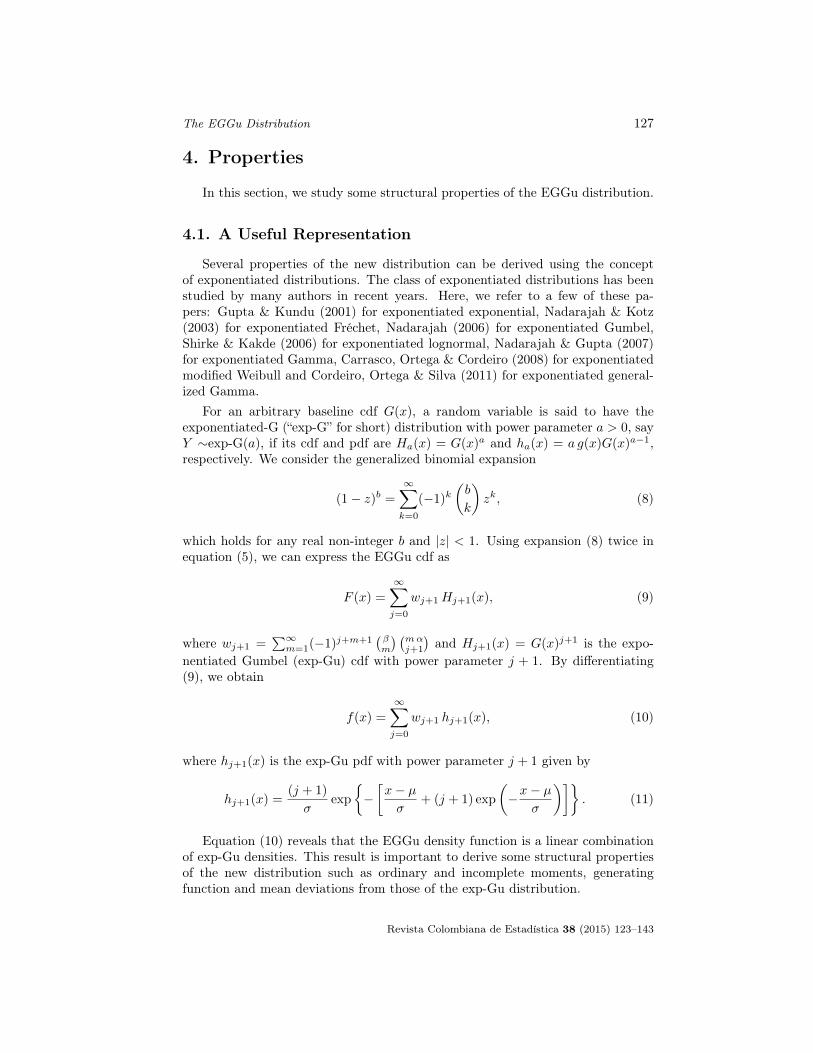
Plots of the EGGu density function for selected parameter values are displayedin Figure 1.
−2 −1 0 1 2 3 4
0.0
0.2
0.4
0.6
0.8
1.0
β = 1
x
Den
sity
α = 2α = 3α = 4α = 5
−2 −1 0 1 2 3 4
0.0
0.2
0.4
0.6
0.8
1.0
β = 5
x
Den
sity
α = 2α = 3α = 4α = 5
−2 −1 0 1 2 3 4
0.0
0.5
1.0
1.5
α = 2
x
Den
sity
β = 3β = 5β = 7β = 9
−2.0 −1.5 −1.0 −0.5 0.0 0.5 1.0
0.0
0.5
1.0
1.5α = 9
x
Den
sity
β = 3β = 5β = 7β = 9
Figure 1: Plots of the EGGu pdf for µ = 0, σ = 1 and some values of α and β.
Revista Colombiana de Estadística 38 (2015) 123–143
The EGGu Distribution 127
4. Properties
In this section, we study some structural properties of the EGGu distribution.
4.1. A Useful Representation
Several properties of the new distribution can be derived using the conceptof exponentiated distributions. The class of exponentiated distributions has beenstudied by many authors in recent years. Here, we refer to a few of these pa-pers: Gupta & Kundu (2001) for exponentiated exponential, Nadarajah & Kotz(2003) for exponentiated Fréchet, Nadarajah (2006) for exponentiated Gumbel,Shirke & Kakde (2006) for exponentiated lognormal, Nadarajah & Gupta (2007)for exponentiated Gamma, Carrasco, Ortega & Cordeiro (2008) for exponentiatedmodified Weibull and Cordeiro, Ortega & Silva (2011) for exponentiated general-ized Gamma.
For an arbitrary baseline cdf G(x), a random variable is said to have theexponentiated-G (“exp-G” for short) distribution with power parameter a > 0, sayY ∼exp-G(a), if its cdf and pdf are Ha(x) = G(x)a and ha(x) = a g(x)G(x)a−1,respectively. We consider the generalized binomial expansion
(1− z)b =
∞∑k=0
(−1)k(b
k
)zk, (8)
which holds for any real non-integer b and |z| < 1. Using expansion (8) twice inequation (5), we can express the EGGu cdf as
F (x) =
∞∑j=0
wj+1Hj+1(x), (9)
where wj+1 =∑∞m=1(−1)j+m+1
(βm
) (mαj+1
)and Hj+1(x) = G(x)j+1 is the expo-
nentiated Gumbel (exp-Gu) cdf with power parameter j + 1. By differentiating(9), we obtain
f(x) =
∞∑j=0
wj+1 hj+1(x), (10)
where hj+1(x) is the exp-Gu pdf with power parameter j + 1 given by
hj+1(x) =(j + 1)
σexp
{−[x− µσ
+ (j + 1) exp
(−x− µ
σ
)]}. (11)
Equation (10) reveals that the EGGu density function is a linear combinationof exp-Gu densities. This result is important to derive some structural propertiesof the new distribution such as ordinary and incomplete moments, generatingfunction and mean deviations from those of the exp-Gu distribution.
Revista Colombiana de Estadística 38 (2015) 123–143
128 Thiago Andrade, Heloisa Rodrigues, Marcelo Bourguignon & Gauss Cordeiro
4.2. Quantile function
In applied work, we are interested on the quantile function (qf) of a continuousdistribution. Based on the qf, we can generate occurrences of the distribution andobtain measures of skewness and kurtosis. The EGGu qf, say x = Q(u), followsby inverting the EGGu cdf (5) as
x = Q(u) = µ− σ log{− log[1− (1− u1/β)1/α]}. (12)
The median of X is simply x1/2 = Q(1/2). Further, it is possible to generateEGGu variates by X = Q(U), where U is a uniform variate on the unit interval(0, 1).
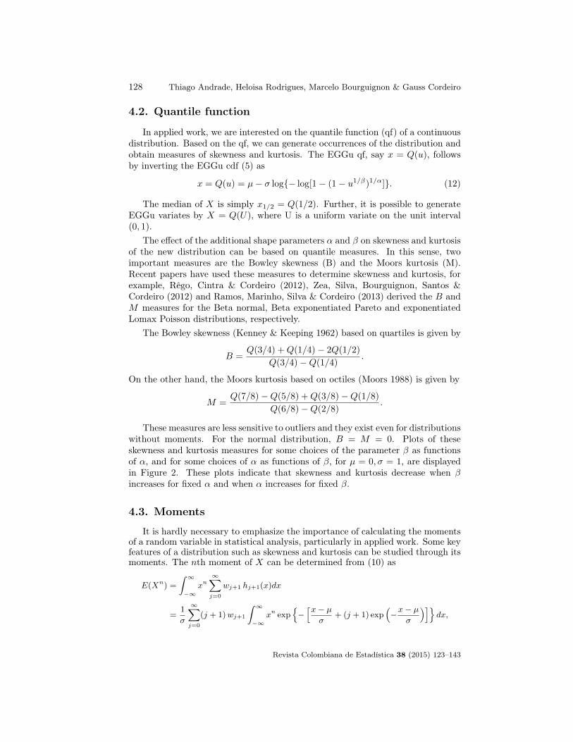
The effect of the additional shape parameters α and β on skewness and kurtosisof the new distribution can be based on quantile measures. In this sense, twoimportant measures are the Bowley skewness (B) and the Moors kurtosis (M).Recent papers have used these measures to determine skewness and kurtosis, forexample, Rêgo, Cintra & Cordeiro (2012), Zea, Silva, Bourguignon, Santos &Cordeiro (2012) and Ramos, Marinho, Silva & Cordeiro (2013) derived the B andM measures for the Beta normal, Beta exponentiated Pareto and exponentiatedLomax Poisson distributions, respectively.
The Bowley skewness (Kenney & Keeping 1962) based on quartiles is given by
B =Q(3/4) +Q(1/4)− 2Q(1/2)
Q(3/4)−Q(1/4).
On the other hand, the Moors kurtosis based on octiles (Moors 1988) is given by
M =Q(7/8)−Q(5/8) +Q(3/8)−Q(1/8)
Q(6/8)−Q(2/8).
These measures are less sensitive to outliers and they exist even for distributionswithout moments. For the normal distribution, B = M = 0. Plots of theseskewness and kurtosis measures for some choices of the parameter β as functionsof α, and for some choices of α as functions of β, for µ = 0, σ = 1, are displayedin Figure 2. These plots indicate that skewness and kurtosis decrease when βincreases for fixed α and when α increases for fixed β.
4.3. Moments
It is hardly necessary to emphasize the importance of calculating the momentsof a random variable in statistical analysis, particularly in applied work. Some keyfeatures of a distribution such as skewness and kurtosis can be studied through itsmoments. The nth moment of X can be determined from (10) as
E(Xn) =
∫ ∞−∞
xn∞∑j=0
wj+1 hj+1(x)dx
=1
σ
∞∑j=0
(j + 1)wj+1
∫ ∞−∞
xn exp{−[x− µ
σ+ (j + 1) exp
(−x− µ
σ
)]}dx,
Revista Colombiana de Estadística 38 (2015) 123–143
The EGGu Distribution 129
1 2 3 4 5
0.04
0.06
0.08
0.10
0.12
0.14
0.16
α
Ske
wne
ss
β = 1β = 2β = 3β = 4
1 2 3 4 5
0.14
0.16
0.18
0.20
0.22
0.24
0.26
0.28
β
Ske
wne
ss
α = 0.2α = 0.3α = 0.4α = 0.5
1 2 3 4 5
1.24
1.25
1.26
1.27
1.28
1.29
1.30
1.31
α
Kur
tosi
s
β = 1β = 2β = 3β = 4
1 2 3 4 5
1.30
1.35
1.40
β
Kur
tosi
s
α = 0.2α = 0.3α = 0.4α = 0.5
Figure 2: Plots of the EGGu skewness and kurtosis as functions of α for some valuesof β and as functions of β for some values of α.
which, on setting u = exp{−(x− µ)/σ}, it reduces to
E(Xn) =∞∑j=0
(j + 1)wj+1
∫ ∞0
[µ− σ log(u)]n exp{−u(j + 1)}du.
Using the binomial expansion for [µ− σ log(u)]n, E(Xn) can be expressed as
E(Xn) =
∞∑j=0
n∑i=0
(j+ 1)
(n
i
)(−σ)iµn−iwj+1
∫ ∞0
[log(u)]i exp{−u(j+ 1)}du. (13)
Using a result by Nadarajah (2006), I(i, j) =∫∞0
[log(u)]i exp{−u(j + 1)}dureduces to
I(i, j) =
(∂
∂a
)i[(j + 1)−aΓ(a)] |a=1 . (14)
Revista Colombiana de Estadística 38 (2015) 123–143
130 Thiago Andrade, Heloisa Rodrigues, Marcelo Bourguignon & Gauss Cordeiro
By combining (13) and (14), the nth moment of X becomes
E(Xn) =
∞∑j=0
n∑i=0
(j + 1)
(n
i
)(−σ)iµn−i wj+1
(∂
∂a
)i[(j + 1)−aΓ(a)] |a=1 .
4.4. Generating Function
The moment generating function (mgf) of X can be obtained using the factthat the EGGu density function is a linear combination of exp-Gu densities. Thus,
M(t) =
∞∑j=0
wj+1
∫ ∞−∞
etx hj+1(x)dx
=1
σ
∞∑j=0
(j + 1)wj+1
∫ ∞−∞
etx exp
{−[x− µσ
+ (j + 1) exp
(−x− µ
σ
)]}dx.
Setting u = exp{−(x− µ)/σ}, M(t) reduces to
M(t) = etµ∞∑j=0
(j + 1)wj+1
∫ ∞0
u−tσ exp[−(j + 1)u] du.
Using a result by Cordeiro et al. (2012), we have
I(j) =
∫ ∞0
u−tσ exp[−(j + 1)u] du = Γ(1− tσ)(j + 1)tσ−1,
and then
M(t) = etµ Γ(1− tσ)
∞∑j=0
(j + 1)tσ wj+1.
4.5. Mean Deviations
Generally, there has been a great interest in obtaining the first incompletemoment of a distribution. Based on this quantity, we can calculate, for example,mean deviations which provide important information about the characteristics ofa population. Indeed, the amount of dispersion in a population may be measuredto some extent by all the deviations from the mean and the median.
For calculating the mean deviations from the mean and the median, we requirethe first incomplete moment of X given by T (z) =
∫ z−∞ x f(x) dx. Using equation
(10) and setting u = exp{−(x− µ)/σ}, T (z) reduces to
Revista Colombiana de Estadística 38 (2015) 123–143
The EGGu Distribution 131
T (z) =
∞∑j=0
(j + 1)wj+1
∫ ∞t
[µ− σ log(u)] exp[−u(j + 1)]du
=
∞∑j=0
wj+1{exp[−t(j + 1)][µ− σ log(t)]− σΓ[0, (j + 1)t]},(15)
where t = exp{−(z − µ)/σ} and Γ(k, x) =∫∞xvk−1 e−vdv is the complementary
incomplete Gamma function.The mean deviations from the mean and the median are defined by
δ1 = 2µ′1 F (µ′1)− 2T (µ′1) and δ2 = µ′1 − 2T (M),
respectively, where µ′1 = E(X), the median M of X is determined from the qf byM = Q(1/2), F (M) and F (µ′1) are easily obtained from (5) and T (z) is given by(15).
Another important application of the first incomplete moment is to determineBonferroni and Lorenz curves, which are commonly used in applied works in areassuch as economics, reliability, demography, insurance, medicine and others. For agiven probability π, these curves are defined by B(π) = T (q)/(πµ′1) and L(π) =T (q)/µ′1, where µ′1 = E(X) and q = Q(π) is calculated by (12).
4.6. Rényi Entropy
The entropy of a random variable X with density function f(x) is a measureof variation of the uncertainty. For any real parameter λ > 0 and λ 6= 1, the Rényientropy is given by
IR(λ) =1
(1− λ)log
(∫ ∞−∞
f(x)λdx
).
Using the binomial expansion (8) twice in equation (4), we can write
f(x)λ = (αβ)λ∞∑j=0
δj G(x)j g(x)λ, (16)
where δj is given by
δj =
∞∑i=0
(−1)i+j(λ(β − 1)
i
)(αi+ λ(α− 1)
j
).
Inserting (1) and (2) in equation (16) and after some algebra, we obtain
f(x)λ =
(αβ
σ
)λ ∞∑j=0
δj exp
{−[λ(x− µ)
σ+ (j + λ) exp
(−x− µ
σ
)]}.
Revista Colombiana de Estadística 38 (2015) 123–143
132 Thiago Andrade, Heloisa Rodrigues, Marcelo Bourguignon & Gauss Cordeiro
Finally,
IR(λ) =1
(1− λ)log
{(αβ
σ
)λ ∞∑j=0
δj×
∫ ∞−∞
exp
{−[λ(x− µ)
σ+ (j + λ) exp
(−x− µ
σ
)]}dx
}.
4.7. Order statistics
We derive an explicit expression for the density of the ith order statistic Xi:n,say fi:n(x), in a random sample of size n from the EGGu distribution. It is well-known that
fi:n(x) =1
B(i, n− i+ 1)
n−i∑j=0
(−1)j(n− ij
)f(x)F (x)i+j−1. (17)
Substituting (3) and (4) in equation (17) and applying the binomial expansion(8) twice, we can write
fi:n(x) =αβ
B(i, n− i+ 1)
∞∑`=0
ϑ` g(x)G(x)`,
where ϑ` is given by
ϑ` =
n−i∑j=0
∞∑k=0
(−1)j+k+`(n− ij
)(β(i+ j)− 1
k
)(α(k + 1)− 1
`
).
Thus, replacing G(x) and g(x) by the cdf and pdf of the Gumbel distributiongiven by (1) and (2), respectively, we can write fi:n(x) as
fi:n(x) =αβ
σB(i, n− i+ 1)
∞∑`=0
ϑ` exp
{−[x− µσ
+ (`+ 1) exp
(−x− µ
σ
)]}.
After simple algebraic manipulation, we can rewrite the last equation as
fi:n(x) =αβ
B(i, n− i+ 1)
∞∑`=0
ϑ∗` h`+1(x), (18)
where ϑ∗` = ϑ`/(`+ 1) and h`+1(x) is given by (11).Equation (18) reveals that the density function of the EGGu order statistic is a
linear combination of exp-Gu densities. A direct application of (18) is to calculatethe moments and the mgf of the EGGu order statistics.
The rth moment of Xi:n is given by
E(Xri:n) =
αβ
B(i, n− i+ 1)
∞∑`=0
ϑ∗`
∫ ∞−∞
xr h`+1(x) dx.
Revista Colombiana de Estadística 38 (2015) 123–143
The EGGu Distribution 133
From the results presented in Section 4.3, the last equation reduces to
E(Xri:n) =
αβ
B(i, n− i+ 1)
∞∑`=0
r∑k=0
(`+ 1) (−σ)k µr−k(rk
)ϑ∗`
(∂
∂a
)k[(`+ 1)−aΓ(a)] |a=1 .
The mgf of Xi:n is given by
M(t) =αβ
B(i, n− i+ 1)
∞∑`=0
ϑ∗`
∫ ∞−∞
etx h`+1(x) dx.
Finally, based on the results in Section 4.4, the last equation can be rewrittenas
M(t) =αβ etµ Γ(1− tσ)
B(i, n− i+ 1)
∞∑`=0
(`+ 1)tσ ϑ∗` .
5. Estimation
Several approaches for parameter point estimation were proposed in the liter-ature but the maximum likelihood method is the most commonly employed. TheMLEs enjoy desirable properties and can be used when constructing confidenceintervals and regions and also in test statistics. Large sample theory for theseestimates delivers simple approximations that work well in finite samples. Theresulting approximation for the estimates in distribution theory is easily handledeither analytically or numerically. So, we consider the estimation of the unknownparameters α, β, µ and σ of the EGGu distribution from complete samples onlyby the method of maximum likelihood. Let x1, . . . , xn be a sample of size n fromX. The log-likelihood function for the vector of parameters θ> = (α, β, µ, σ)> canbe expressed as
`(θ) = n log
(αβ
σ
)−
n∑i=1
[xi − µσ
+ exp
(−xi − µ
σ
)]
+ (α− 1)
n∑i=1
log
{1− exp
[− exp
(−xi − µ
σ
)]}
+ (β − 1)
n∑i=1
log
{1−
[1− exp
[− exp
(−xi − µ
σ
)]]α}.
The elements of the score vector are given by
∂`(θ)
∂α=n
α+
n∑i=1
log[H(xi)] + (1− β)
n∑i=1
H(xi)α logH(xi)
1−H(xi)α,
∂`(θ)
∂β=n
β+
n∑i=1
log[1−H(xi)α],
Revista Colombiana de Estadística 38 (2015) 123–143
134 Thiago Andrade, Heloisa Rodrigues, Marcelo Bourguignon & Gauss Cordeiro
∂`(θ)
∂µ=n
σ− 1
σ
n∑i=1
exp
(−xi − µ
σ
)+ (α− 1)
n∑i=1
g(xi)
H(xi)
+ α(1− β)
n∑i=1
g(xi)H(xi)α−1
1−H(xi)α,
∂`(θ)
∂σ= −nµ
σ2− n
σ− 1
σ2
n∑i=1
(xi − µ) exp
(−xi − µ
σ
)+
1
σ2
n∑i=1
xi
+ (α− 1)
n∑i=1
(xi − µ)g(xi)
σH(xi)
+ (β − 1)
n∑i=1
−α(xi − µ)g(xi)H(x)α−1
σ[1−H(x)α],
whereH(xi) = 1− exp
[− exp
(−xi − µ
σ
)]and
g(xi) =1
σexp
{−[xi − µσ
+ exp
(−xi − µ
σ
)]}.
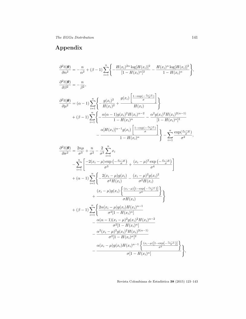
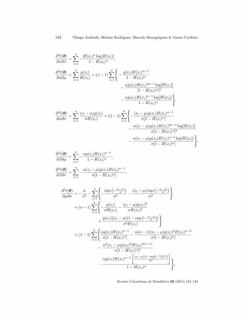
The maximum likelihood estimate (MLE) θ̂ of θ is obtained by solving nonlinearequations Uα(θ) = 0, Uβ(θ) = 0, Uµ(θ) = 0 and Uσ(θ) = 0. They cannot be solvedanalytically and require statistical software with iterative numerical techniques.There are many maximization methods in R scripts like NR (Newton-Raphson),BFGS (Broyden-Fletcher-Goldfarb-Shanno), BHHH (Berndt-Hall-Hall-Hausman),SANN (Simulated-Annealing), NM (Nelder-Mead) and L-BFGS-B. For intervalestimation and hypothesis tests on the parameters α, β, µ and σ, we determine the4× 4 observed information matrix J(θ) = {−Urs}, where Urs = ∂2`(θ)/(∂θr∂θs)for r, s ∈ {α, β, µ, σ}. The elements of J(θ) are given in the Appendix.
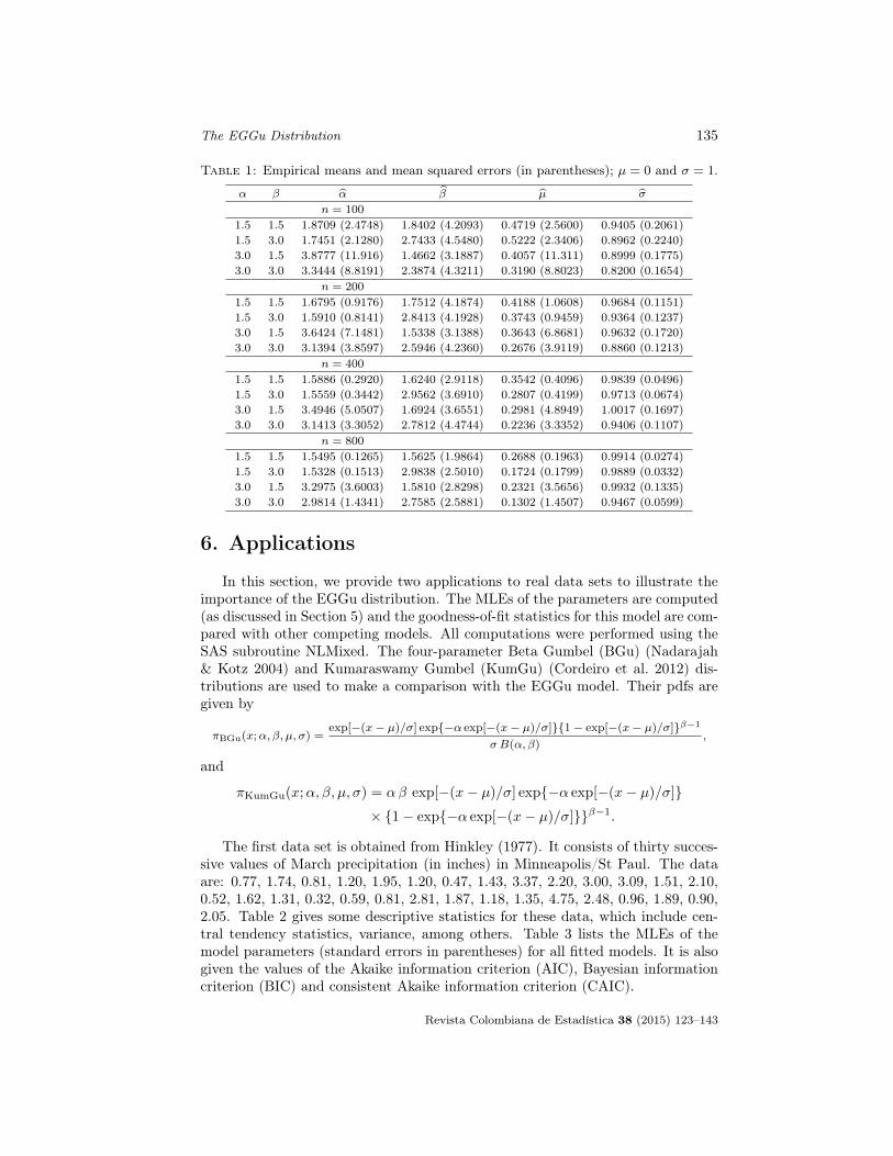
Next, a small Monte Carlo simulation experiment based on 10, 000 replicationswill be conducted to evaluate the MLEs of the parameters of the EGGu distri-bution. We set the sample size at n = 100, 200, 400 and 800, the parameter α atα = 1.5 and 3.0, and the parameter β at β = 1.5 and 3.0. The location and scaleparameters were fixed at µ = 0 and σ = 1, respectively, without loss of generality.The Monte Carlo simulation experiments are performed using the R programminglanguage; see http://www.r-project.org. Table 1 reports the empirical meansand the mean squared errors (in parentheses) of the corresponding estimators.From these figures in this table, we note that, as the sample size increases, theempirical biases and mean squared errors decrease in all the cases analyzed, asexpected.
Revista Colombiana de Estadística 38 (2015) 123–143
The EGGu Distribution 135
Table 1: Empirical means and mean squared errors (in parentheses); µ = 0 and σ = 1.
α β α̂ β̂ µ̂ σ̂
n = 100
1.5 1.5 1.8709 (2.4748) 1.8402 (4.2093) 0.4719 (2.5600) 0.9405 (0.2061)1.5 3.0 1.7451 (2.1280) 2.7433 (4.5480) 0.5222 (2.3406) 0.8962 (0.2240)3.0 1.5 3.8777 (11.916) 1.4662 (3.1887) 0.4057 (11.311) 0.8999 (0.1775)3.0 3.0 3.3444 (8.8191) 2.3874 (4.3211) 0.3190 (8.8023) 0.8200 (0.1654)
n = 200
1.5 1.5 1.6795 (0.9176) 1.7512 (4.1874) 0.4188 (1.0608) 0.9684 (0.1151)1.5 3.0 1.5910 (0.8141) 2.8413 (4.1928) 0.3743 (0.9459) 0.9364 (0.1237)3.0 1.5 3.6424 (7.1481) 1.5338 (3.1388) 0.3643 (6.8681) 0.9632 (0.1720)3.0 3.0 3.1394 (3.8597) 2.5946 (4.2360) 0.2676 (3.9119) 0.8860 (0.1213)
n = 400
1.5 1.5 1.5886 (0.2920) 1.6240 (2.9118) 0.3542 (0.4096) 0.9839 (0.0496)1.5 3.0 1.5559 (0.3442) 2.9562 (3.6910) 0.2807 (0.4199) 0.9713 (0.0674)3.0 1.5 3.4946 (5.0507) 1.6924 (3.6551) 0.2981 (4.8949) 1.0017 (0.1697)3.0 3.0 3.1413 (3.3052) 2.7812 (4.4744) 0.2236 (3.3352) 0.9406 (0.1107)
n = 800
1.5 1.5 1.5495 (0.1265) 1.5625 (1.9864) 0.2688 (0.1963) 0.9914 (0.0274)1.5 3.0 1.5328 (0.1513) 2.9838 (2.5010) 0.1724 (0.1799) 0.9889 (0.0332)3.0 1.5 3.2975 (3.6003) 1.5810 (2.8298) 0.2321 (3.5656) 0.9932 (0.1335)3.0 3.0 2.9814 (1.4341) 2.7585 (2.5881) 0.1302 (1.4507) 0.9467 (0.0599)
6. Applications
In this section, we provide two applications to real data sets to illustrate theimportance of the EGGu distribution. The MLEs of the parameters are computed(as discussed in Section 5) and the goodness-of-fit statistics for this model are com-pared with other competing models. All computations were performed using theSAS subroutine NLMixed. The four-parameter Beta Gumbel (BGu) (Nadarajah& Kotz 2004) and Kumaraswamy Gumbel (KumGu) (Cordeiro et al. 2012) dis-tributions are used to make a comparison with the EGGu model. Their pdfs aregiven by
πBGu(x;α, β, µ, σ) =exp[−(x− µ)/σ] exp{−α exp[−(x− µ)/σ]}{1− exp[−(x− µ)/σ]}β−1
σ B(α, β),
and
πKumGu(x;α, β, µ, σ) = αβ exp[−(x− µ)/σ] exp{−α exp[−(x− µ)/σ]}× {1− exp{−α exp[−(x− µ)/σ]}}β−1.
The first data set is obtained from Hinkley (1977). It consists of thirty succes-sive values of March precipitation (in inches) in Minneapolis/St Paul. The dataare: 0.77, 1.74, 0.81, 1.20, 1.95, 1.20, 0.47, 1.43, 3.37, 2.20, 3.00, 3.09, 1.51, 2.10,0.52, 1.62, 1.31, 0.32, 0.59, 0.81, 2.81, 1.87, 1.18, 1.35, 4.75, 2.48, 0.96, 1.89, 0.90,2.05. Table 2 gives some descriptive statistics for these data, which include cen-tral tendency statistics, variance, among others. Table 3 lists the MLEs of themodel parameters (standard errors in parentheses) for all fitted models. It is alsogiven the values of the Akaike information criterion (AIC), Bayesian informationcriterion (BIC) and consistent Akaike information criterion (CAIC).
Revista Colombiana de Estadística 38 (2015) 123–143
136 Thiago Andrade, Heloisa Rodrigues, Marcelo Bourguignon & Gauss Cordeiro
Table 2: Descriptives statistics for Hinkley’s data set.
StatisticMean 1.675Median 1.470Variance 1.001Minimum 0.320Maximum 4.750
Table 3: MLEs (and the corresponding standard errors in parentheses), AIC, BIC andCAIC statistics for Hinkley’s data.
Distribution α̂ β̂ µ̂ σ̂ AIC BIC CAICEGGu 0.1440 2.1935 0.2190 0.1285 84.1 85.7 89.7
(0.0358)a (1.3392) (0.2508) (0.0078)BGu 0.8294 0.4449 0.9133 0.4301 84.7 86.3 90.3
(2.0008)a (0.4855) (1.5573) (0.3628)KumGu 0.7632 0.4349 0.9225 0.4206 84.7 86.3 90.3
(0.2094)a (0.4428) (0.3800) (0.3151)aDenotes the standard deviations of the MLEs of α, β, µ and σ.
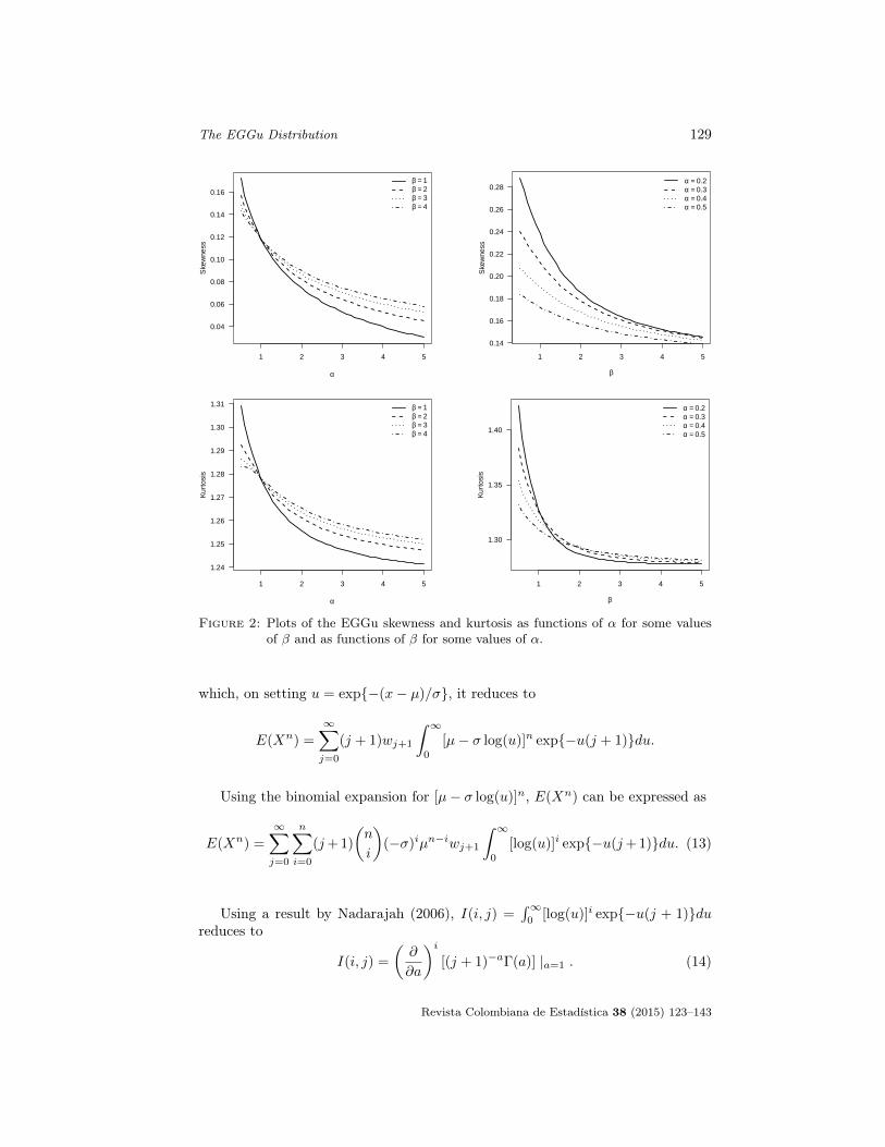
Plots of the estimated pdf and cdf of the fitted EGGu, BGu and KumGumodels to these data are displayed in Figure 3. They indicate that the EGGudistribution is superior to the other distributions in terms of model fitting.
Next, we shall apply formal goodness-of-fit tests in order to verify which distri-bution better fits the current data. We consider the Cramér-von Mises (CM) andAnderson-Darling (AD) statistics, which are described in Chen & Balakrishnan(1995). Table 4 gives the values of the CM and AD statistics (and the p-valuesof the tests in parentheses) for the fitted models. Thus, according to these for-mal tests, the EGGu model fits the current data better than the other models,i.e., these values indicate that the null hypothesis is strongly not rejected for theEGGu distribution. Based on the plots of Figure 3, we conclude that the EGGudistribution provides a better fit to these data than the BGu and KumGu models.
Table 4: Goodness-of-fit tests.
ModelStatistics
CM ADEGGu 0.0151 (0.9932)a 0.1169 (0.9891)a
BGu 0.0205 (0.9611) 0.1606 (0.9415)KumGu 0.0193 (0.9718) 0.1520 (0.9548)aDenotes the p-value of the test.
The second data set is given by Murthy, Xie & Jiang (2004). The data refer thetime between failures for repairable item: 1.43, 0.11, 0.71, 0.77, 2.63, 1.49, 3.46,2.46, 0.59, 0.74, 1.23, 0.94, 4.36, 0.40, 1.74, 4.73, 2.23, 0.45, 0.70, 1.06, 1.46, 0.30,1.82, 2.37, 0.63, 1.23, 1.24, 1.97, 1.86, 1.17. Table 5 gives some descriptive statisticsfor these data. Table 6 gives the MLEs of the model parameters (standard errorsin parentheses) for all fitted models and the values of the AIC, BIC and CAICstatistics.
Revista Colombiana de Estadística 38 (2015) 123–143
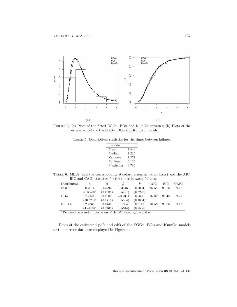
The EGGu Distribution 137
x
Den
sity
0 1 2 3 4 5
0.0
0.1
0.2
0.3
0.4
0.5
EGGuBGuKumGu
(a)
0 1 2 3 4 5
0.0
0.2
0.4
0.6
0.8
1.0
x
cdf
EGGuBGuKumGu
(b)
Figure 3: (a) Plots of the fitted EGGu, BGu and KumGu densities; (b) Plots of theestimated cdfs of the EGGu, BGu and KumGu models.
Table 5: Descriptives statistics for the times between failures.
StatisticMean 1.543Median 1.235Variance 1.272Minimum 0.110Maximum 4.730
Table 6: MLEs (and the corresponding standard errors in parentheses) and the AIC,BIC and CAIC statistics for the times between failures.
Distribution α̂ β̂ µ̂ σ̂ AIC BIC CAICEGGu 0.2914 1.3294 0.3146 0.3004 87.55 93.16 89.15
(0.3659)a (1.0088) (0.5421) (0.3222)BGu 7.7144 0.2089 −0.2351 0.2600 87.82 93.43 89.42
(10.521)a (0.1715) (0.5534) (0.1884)KumGu 2.4766 0.2749 0.1804 0.3115 87.55 93.16 89.15
(4.4419)a (0.2469) (0.5544) (0.2508)aDenotes the standard deviation of the MLEs of α, β, µ and σ.
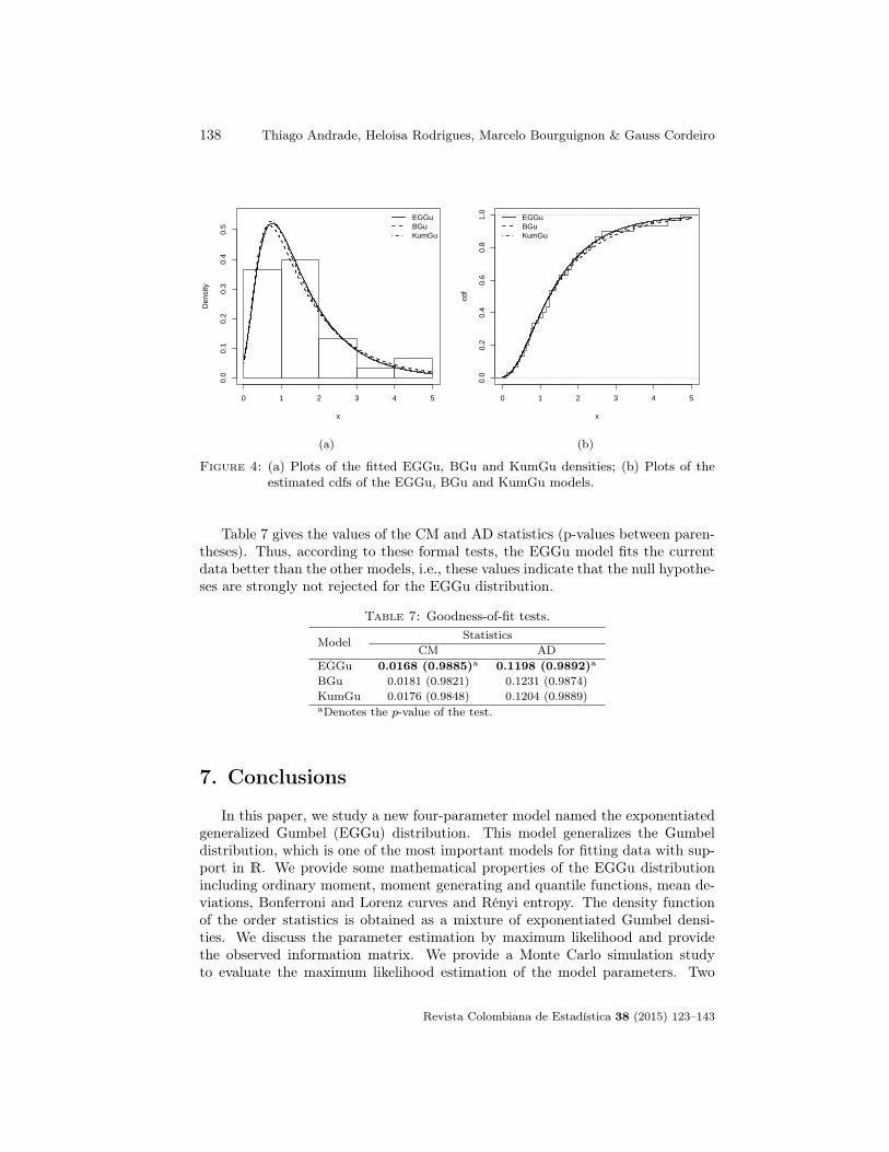
Plots of the estimated pdfs and cdfs of the EGGu, BGu and KumGu modelsto the current data are displayed in Figure 4.
Revista Colombiana de Estadística 38 (2015) 123–143
138 Thiago Andrade, Heloisa Rodrigues, Marcelo Bourguignon & Gauss Cordeiro
x
Den
sity
0 1 2 3 4 5
0.0
0.1
0.2
0.3
0.4
0.5
EGGuBGuKumGu
(a)
0 1 2 3 4 5
0.0
0.2
0.4
0.6
0.8
1.0
x
cdf
EGGuBGuKumGu
(b)
Figure 4: (a) Plots of the fitted EGGu, BGu and KumGu densities; (b) Plots of theestimated cdfs of the EGGu, BGu and KumGu models.
Table 7 gives the values of the CM and AD statistics (p-values between paren-theses). Thus, according to these formal tests, the EGGu model fits the currentdata better than the other models, i.e., these values indicate that the null hypothe-ses are strongly not rejected for the EGGu distribution.
Table 7: Goodness-of-fit tests.
ModelStatistics
CM ADEGGu 0.0168 (0.9885)a 0.1198 (0.9892)a
BGu 0.0181 (0.9821) 0.1231 (0.9874)KumGu 0.0176 (0.9848) 0.1204 (0.9889)aDenotes the p-value of the test.
7. Conclusions
In this paper, we study a new four-parameter model named the exponentiatedgeneralized Gumbel (EGGu) distribution. This model generalizes the Gumbeldistribution, which is one of the most important models for fitting data with sup-port in R. We provide some mathematical properties of the EGGu distributionincluding ordinary moment, moment generating and quantile functions, mean de-viations, Bonferroni and Lorenz curves and Rényi entropy. The density functionof the order statistics is obtained as a mixture of exponentiated Gumbel densi-ties. We discuss the parameter estimation by maximum likelihood and providethe observed information matrix. We provide a Monte Carlo simulation studyto evaluate the maximum likelihood estimation of the model parameters. Two
Revista Colombiana de Estadística 38 (2015) 123–143
The EGGu Distribution 139
applications to real data indicate that the EGGu distribution provides a good fitand can be used as a competitive model to fit real data.
Acknowledgements
We thank two anonymous referees and the associate editor for their valuablesuggestions, which certainly contributed to the improvement of this paper.[
Received: December 2013 — Accepted: October 2014]
References
Carrasco, J. M. F., Ortega, E. M. M. & Cordeiro, G. M. (2008), ‘A generalizedmodified Weibull distribution for lifetime modeling’, Computational Statisticsand Data Analysis 53, 450–462.
Chen, G. & Balakrishnan, N. (1995), ‘A general purpose approximate goodness-of-fit test’, Journal of Quality Technology 27, 154–161.
Cordeiro, G. M. & de Castro, M. (2011), ‘A new family of generalized distribu-tions’, Journal of Statistical Computation and Simulation 81, 883–893.
Cordeiro, G. M., Nadarajah, S. & Ortega, E. M. M. (2012), ‘The KumaraswamyGumbel distribution’, Statistical Methods and Applications 21, 139–168.
Cordeiro, G. M., Ortega, E. M. M. & Cunha, D. C. C. (2013), ‘The exponentiatedgeneralized class of distributions’, Journal of Data Science 11, 1–27.
Cordeiro, G. M., Ortega, E. M. M. & Silva, G. O. (2011), ‘The exponentiatedgeneralized Gamma distribution with application to lifetime data’, Journalof Statistical Computation and Simulation 81, 827–842.
Eugene, N., Lee, C. & Famoye, F. (2002), ‘Beta-normal distribution and its appli-cations’, Communications in Statistics - Theory and Methods 31, 497–512.
Gupta, R. D. & Kundu, D. (2001), ‘Exponentiated exponential distribution: An al-ternative to Gamma and Weibull distributions’, Biometrical Journal 43, 117–130.
Hinkley, D. (1977), ‘On quick choice of power transformations’, The AmericanStatistician 26, 67–69.
Kenney, J. F. & Keeping, E. S. (1962), Mathematics of Statistics, 3 edn, Chapman& Hall Ltd, New Jersey.
Kotz, S. & Nadarajah, S. (2000), Extreme Value Distributions: Theory and Appli-cations, Imperial College Press, London.
Revista Colombiana de Estadística 38 (2015) 123–143
140 Thiago Andrade, Heloisa Rodrigues, Marcelo Bourguignon & Gauss Cordeiro
Marshall, A. N. & Olkin, I. (1997), ‘A new method for adding a parameter toa family of distributions with applications to the exponential and Weibullfamilies’, Biometrika 84, 641–652.
Moors, J. J. (1988), ‘A quantile alternative for kurtosis’, Journal of the RoyalStatistical Society: Series D 37, 25–32.
Murthy, D. N. P., Xie, M. & Jiang, R. (2004), Weibull Models, Wiley series inprobability and statistics, John Wiley & Sons, NJ.
Nadarajah, S. (2006), ‘The exponentiated Gumbel distribution with climate ap-plication’, Environmetrics 17, 13–23.
Nadarajah, S. & Gupta, A. K. (2007), ‘The exponentiated Gamma distributionwith application to drought data’, Calcutta Statistical Association Bulletin59, 29–54.
Nadarajah, S. & Kotz, S. (2003), ‘The exponentiated Fréchet distribution’, Statis-tics on the Internet .*http://interstat.statjournals.net/YEAR/2003/articles/0312002.pdf
Nadarajah, S. & Kotz, S. (2004), ‘The beta Gumbel distribution’, MathematicalProblems in Engineering 4, 323–332.
Ramos, M. W., Marinho, P. R., Silva, R. V. & Cordeiro, G. M. (2013), ‘TheExponentiated Lomax Poisson Distribution with an Application to lifetimedata’, Advances and Applications in Statistics 34, 107–135.
Rêgo, L. C., Cintra, R. J. & Cordeiro, G. M. (2012), ‘On some properties ofthe Beta normal distribution’, Communications in Statistics - Theory andMethods 41, 3722–3738.
Ristic, M. M. & Balakrishnan, N. (2011), ‘The Gamma exponentiated exponen-tial distribution’, Journal of Statistical Computation and Simulation . doi:10.1080/00949655.2011.574633.
Shirke, D. T. & Kakde, C. S. (2006), ‘On exponentiated lognormal distribution’,International Journal of Agricultural and Statistical Sciences 2, 319–326.
Tahir, M. & Nadarajah, S. (2013), ‘Parameter induction in continuous univariatedistributions - Part I: Well-established G-classes’, Communications in Statis-tics - Theory and Methods .
Zea, L. M., Silva, R. B., Bourguignon, M., Santos, A. M. & Cordeiro, G. M. (2012),‘The Beta exponentiated Pareto distribution with application to Bladder Can-cer susceptibility’, International Journal of Statistics and Probability 1, 8–19.
Zografos, K. & Balakrishnan, N. (2009), ‘On families of Beta- and generalizedGamma-generated distributions and associated inference’, Statistical Method-ology 6, 344–362.
Revista Colombiana de Estadística 38 (2015) 123–143
The EGGu Distribution 141
Appendix
∂2`(θ)
∂α2= − n
α2+ (β − 1)
n∑i=1
{−H(xi)
2α log[H(xi)]2
[1−H(xi)α]2− H(xi)
α log[H(xi)]2
1−H(xi)α
},
∂2`(θ)
∂β2= − n
β2,
∂2`(θ)
∂µ2= (α− 1)
n∑i=1
{− g(xi)
2
H(xi)2+
g(xi)
[1−exp(− xi−µσ )
σ
]H(xi)
}
+ (β − 1)
n∑i=1
{−α(α− 1)g(xi)
2H(xi)α−2
1−H(xi)α− α2g(xi)
2H(xi)2(α−1)
[1−H(xi)α]2
−α[H(xi)]
α−1g(xi)
[1−exp(− xi−µσ )
σ
]1−H(xi)α
}−
n∑i=1
exp(xi−µσ )
σ2,
∂2`(θ)
∂σ2=
2nµ
σ3+
n
σ2− 2
σ3
n∑i=1
xi
−n∑i=1
[−2(xi − µ) exp
(−xi−µσ
)σ3
+(xi − µ)2 exp
(−xi−µσ
)σ4
]
+ (α− 1)
n∑i=1
{−2(xi − µ)g(xi)
σ2H(xi)− (xi − µ)2g(xi)
2
σ2H(xi)
+
(xi − µ)g(xi)
{(xi−µ)[1−exp(− xi−µσ )]
σ2
}σH(xi)
}
+ (β − 1)
n∑i=1
{2α(xi − µ)g(xi)H(xi)
α−1
σ2[1−H(xi)α]
− α(α− 1)(xi − µ)2g(xi)2H(xi)
α−2
σ2[1−H(xi)α]
− α2(xi − µ)2g(xi)2H(xi)
2(α−1)
σ2[1−H(xi)α]2
−α(xi − µ)g(xi)H(xi)
α−1{
(xi−µ)[1−exp(− xi−µσ )]σ2
}σ[1−H(xi)α]
},
Revista Colombiana de Estadística 38 (2015) 123–143
142 Thiago Andrade, Heloisa Rodrigues, Marcelo Bourguignon & Gauss Cordeiro
∂2`(θ)
∂α∂β=
n∑i=1
−H(xi)α log[H(xi)]
1−H(xi)α,
∂2`(θ)
∂α∂µ=
n∑i=1
g(xi)
H(xi)+ (β − 1)
n∑i=1
{− g(xi)H(xi)
α−1
1−H(xi)α
− αg(xi)H(xi)2α−1 log[H(xi)]
[1−H(xi)α]2
− αg(xi)H(xi)α−1 log[H(xi)]
1−H(xi)α
},
∂2`(θ)
∂α∂σ=
n∑i=1
(xi − µ)g(xi)
σH(xi)+ (β − 1)
n∑i=1
{− (xi − µ)g(xi)H(xi)
α−1
σ[1−H(xi)α]
− α(xi − µ)g(xi)H(xi)2α−1 log[H(xi)]
σ[1−H(xi)α]2
− α(xi − µ)g(xi)H(xi)α−1 log[H(xi)]
σ[1−H(xi)α]
},
∂2`(θ)
∂β∂µ=
n∑i=1
−αg(xi)H(xi)α−1
1−H(xi)α,
∂2`(θ)
∂β∂σ=
n∑i=1
−α(xi − µ)g(xi)H(xi)α−1
σ[1−H(xi)α],
∂2`(θ)
∂µ∂σ= − n
σ2−
n∑i=1
{−
exp(−xi−µσ
)σ2
−(xi − µ) exp
(−xi−µσ
)σ3
}
+ (α− 1)
n∑i=1
{− g(xi)
σH(xi)− (xi − µ)g(xi)
2
σH(xi)2
+g(xi)[(xi − µ)(1− exp
(−xi−µσ
)]
σ2H(xi)
}
+ (β − 1)
n∑i=1
{αg(xi)H(xi)
α−1
σ[1−H(xi)α]− α(α− 1)(xi − µ)g(xi)
2H(xi)α−2
σ[1−H(xi)α]
− α2(xi − µ)g(xi)2H(xi)
2(α−1)
σ[1−H(xi)α]2
−αg(xi)H(xi)
α−1[(xi−µ)(1−exp(− xi−µσ )
σ2
]1−H(xi)α
},
Revista Colombiana de Estadística 38 (2015) 123–143
The EGGu Distribution 143
whereH(xi) = 1− exp
[− exp
(−xi − µ
σ
)]and
g(xi) =1
σexp
{−[xi − µσ
+ exp
(−xi − µ
σ
)]}.
Revista Colombiana de Estadística 38 (2015) 123–143