1

The Equilibrium Channel& Channel Change

Peter Wilcock3 August 2016

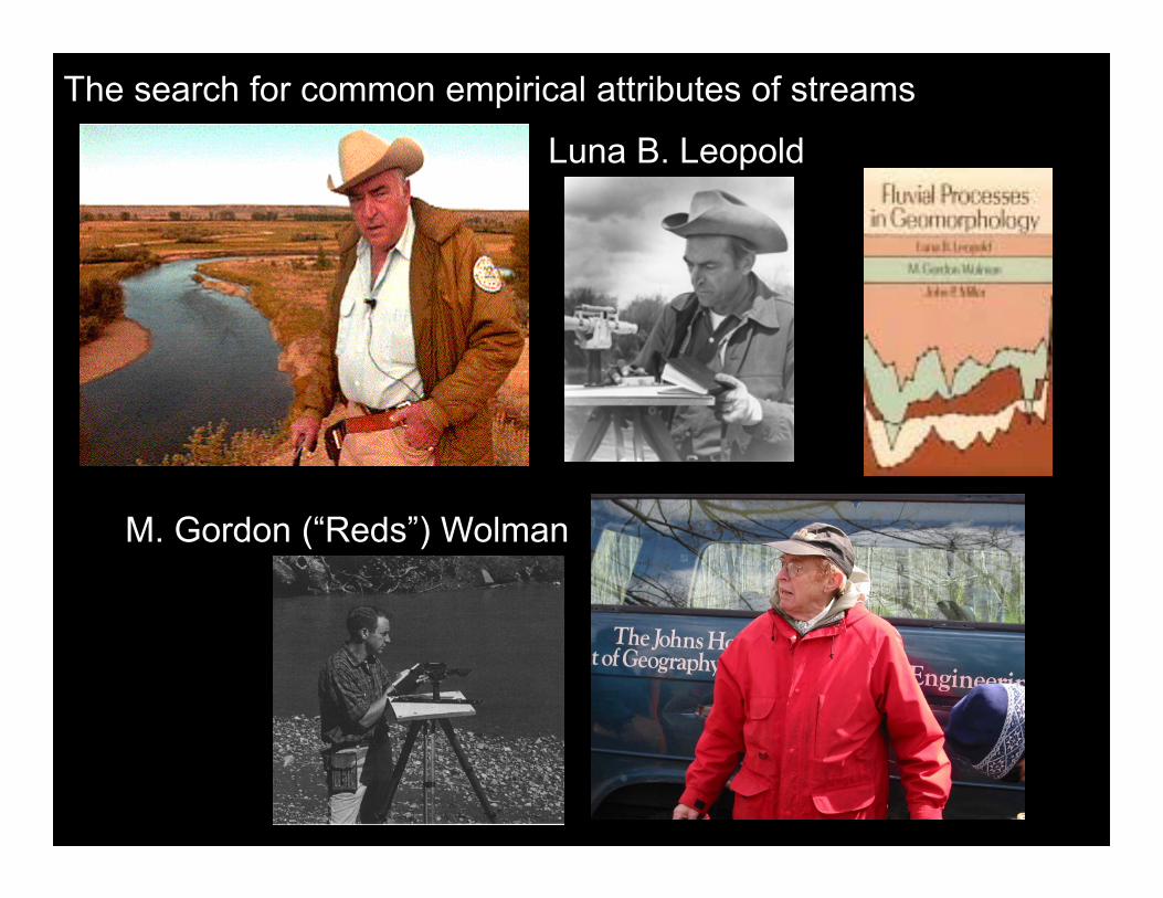
The search for common empirical attributes of streams

Luna B. Leopold

M. Gordon (“Reds”) Wolman

A meandering stream in a wide alluvial valley

Watts Branch, MD

The channel actively migrated across its valley, depositing a point bar on the inside of the meander bends and cutting

a steep bank on the outside of the bends. The upper surface of the point bar was relatively flat.

The remarkable thing was that the channel appeared to 

maintain its size and shape as it migrated.  It appeared to be in a state of dynamic equilibrium.

Active floodplain

And its stratigraphy

The flat surface behind the cutbank is higher than the pointbar floodplain, presumably as the result of gradual overbank deposition during large floods over the period since it was originally deposited.

The architecture of the alluvial valley reflects a competition between lateral accretion and vertical accretion.  At Watts 

Branch, lateral accretion was seen as dominant.

The elevations of the active floodplain have a reach-average slope that is approximately parallel to that of the bed. Terraces are higher than the active

floodplain with elevations that are parallel to the bed as well.

The active floodplain is being constructed in the present hydrologic regime. This landform is inundated by frequent floods. The elevation of flow that just begins to inundate this feature was defined as the bank full stage.

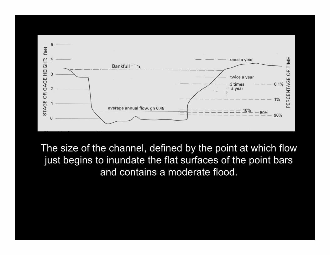
The size of the channel, defined by the point at which flow just begins to inundate the flat surfaces of the point bars

and contains a moderate flood.

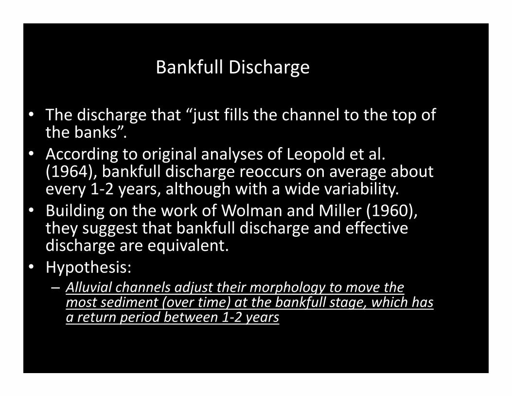
Bankfull Discharge

• The discharge that “just fills the channel to the top of the banks”.

• According to original analyses of Leopold et al. (1964), bankfull discharge reoccurs on average about every 1‐2 years, although with a wide variability.

• Building on the work of Wolman and Miller (1960), they suggest that bankfull discharge and effective discharge are equivalent.

• Hypothesis:– Alluvial channels adjust their morphology to move the most sediment (over time) at the bankfull stage, which has a return period between 1‐2 years

1 10 100Return Period of Bankfull Flow (years)

Wolman and Leopold, 1957 WY, MT, MD, NC, SC, CT

Kilpatrick & Barnes, 1964 AL, GA, NC, SC

Leopold, Wolman, Miller 1964 IN, NB, MS, MD

Williams, 1978 CO, UT, NM, OR

ALL n = 107

2 @ 200 yrs -->

75% of obs within box 1.06 5

19% of obs: 1.36<RI<2.2 yr

Some early studies on the magnitude of bankfull discharge show considerable variability, but a median in the 1‐2 yr range …

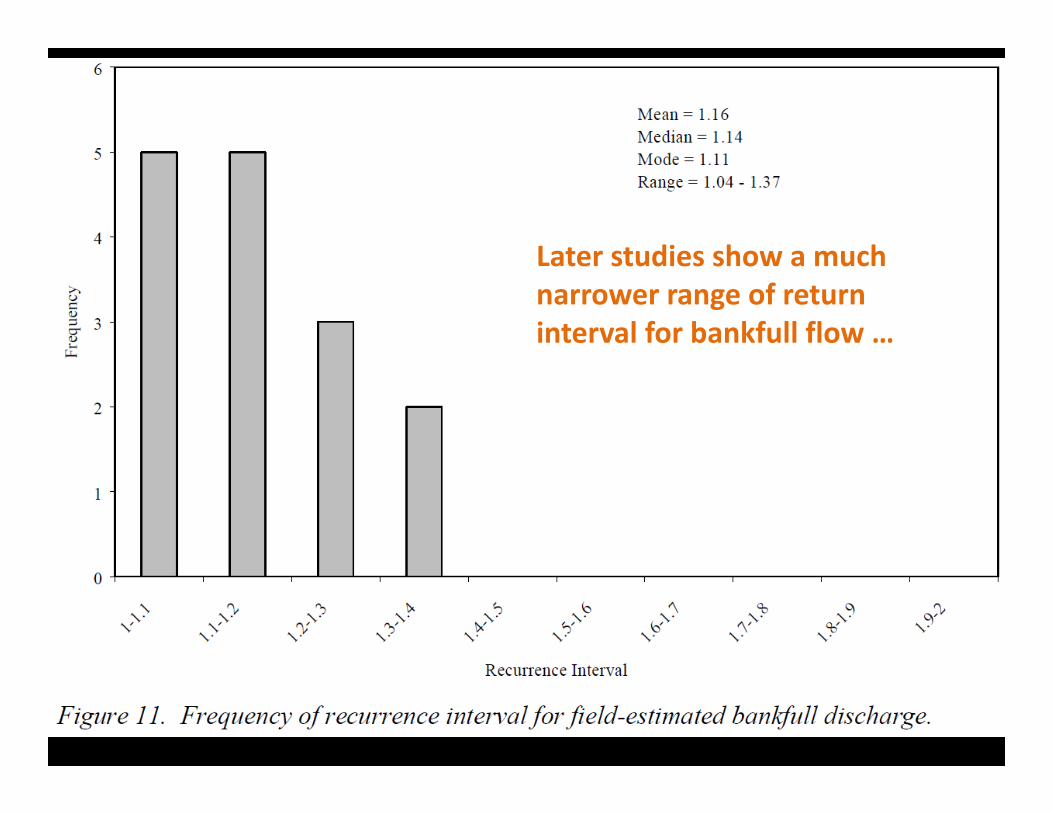
Later studies show a much narrower range of return interval for bankfull flow …

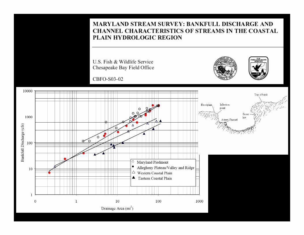
MARYLAND STREAM SURVEY: BANKFULL DISCHARGE AND CHANNEL CHARACTERISTICS OF STREAMSU.S. Fish & Wildlife Service, Chesapeake Bay Field OfficeAPPENDIX B – PROTOCOLS FOR FIELD SURVEYS AT GAGE STATIONS - DETERMINATION OF BANKFULL STAGESteep, confined streams in rocky canyons often lack distinguishable floodplains, so other features must be used.  Where floodplains are absent or poorly defined, other indicators may serve as surrogates to identify bankfull stage. 

Useful indicators include:     Top of Point Bars, Change in Vegetation, Change in Slope, Change in Bank Materials, Bank Undercuts, Stain Lines.

Deposits of pine needles, twigs, and other floating materials are common along streams, but they are seldom indicators of bankfull stage.

If stream gage data is available for the stream, observations of indicators at or near the gages may help to identify the indicators most useful for a particular area. 

Bankfull discharges tend to have similar flow‐frequency (approximately 1.5 years) … among sites in a given climatic region.  Use … observations of bankfull stage at local stream gages to test the reliability of the various indicators for your geographic area. Compare your calculation of bankfull discharge to the regional averages. If it is different, refer to the USGS peak flow procedures for the area to determine if a significantly different area‐runoff relationship exists. In the absence of other reasonable explanations, examine your methods.

The hypothesis that the bankfull channel is adjusted to a flood of return interval 1.0 ‐ to 1.5 yr is now used to select the indicators for the  “bankfull” channel.  The logic has come full circle! The appropriate bankfull indicator is taken to be that corresponding  to a flow with a return interval in the range 1.0 – 1.5 yr.  Regardless of its relevance to channel morphology!  No wonder data on the flood frequency of bankfull channels have become quite tidy… it no longer makes a difference whether one is looking at the top of the bank!

We are no longer looking for the bankfull channel, but for the channel that holds the 1.0 – 1.5 yr flood.One could reasonably ask … for what purpose?  If the bankfull channel is to be used to size a design channel, and the new “bankfull” is nothing more than the 1.0 – 1.5 yr flood, then why not use the return interval as the design criteria?   One could reasonably say, “I want my channel to flood two years out of three” (the 1.5 yr flood).  {or  every other year: the 2‐yr flood. or four years out of five: the 1.25 yr flood}.  There is good reason for considering flood frequency in channel design – but why jump on the bankfull track, which only takes you in circles?  Just specify the desired flood frequency and go with it!

Why is there a focus on equilibrium channel geometry its bankfull flow?

To provide a templatea channel geometry for design

There are a couple of problems …

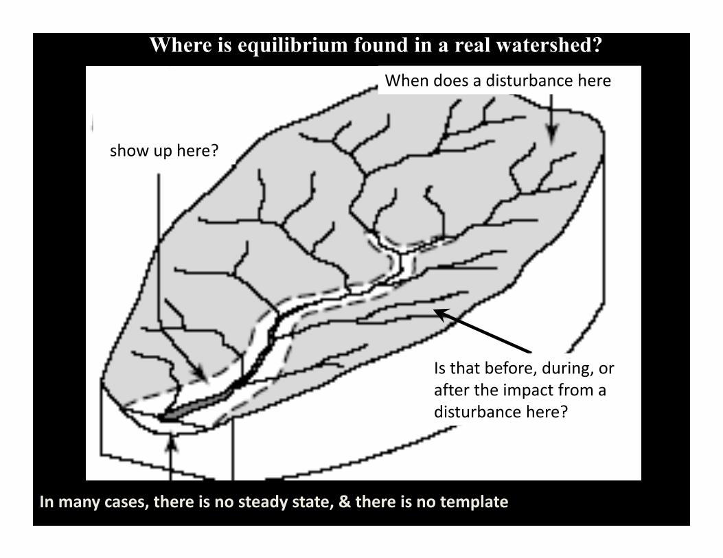
When does a disturbance here

show up here?

Is that before, during, or after the impact from a disturbance here?

Where is equilibrium found in a real watershed?

In many cases, there is no steady state, & there is no template

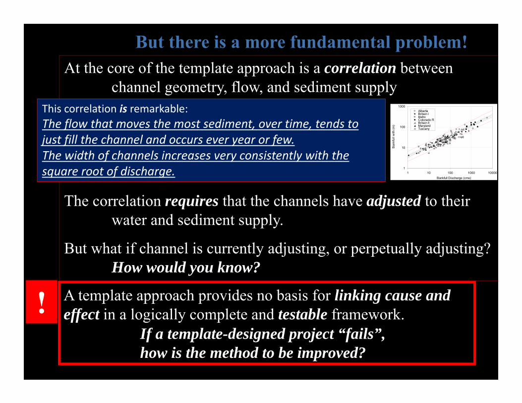
But there is a more fundamental problem!At the core of the template approach is a correlation between

channel geometry, flow, and sediment supply

The correlation requires that the channels have adjusted to theirwater and sediment supply.

But what if channel is currently adjusting, or perpetually adjusting? How would you know?

A template approach provides no basis for linking cause and effect in a logically complete and testable framework.

If a template-designed project “fails”, how is the method to be improved?

!

This correlation is remarkable:The flow that moves the most sediment, over time, tends to just fill the channel and occurs ever year or few.The width of channels increases very consistently with the square root of discharge. 1

10

100

1000

1 10 100 1000 10000

AlbertaBritain IIdahoColorado RBritain IIMarylandTuscany

Bankfull Discharge (cms)

Ban

kful

l with

(m)

18

Understanding Channel Changelinking sediment supply to transport capacitywith a bit of sleepy old Tom Com thrown in

3

33/ 2

3/ 2

3 23

3/ 2

2 2

3/ 2

3/ 4

3/ 422 2 1

1 1 1 2

Einstein-Brown depth-slope continuity Chezy

* ( *)

( )

or

or for two cases

b

b

b

b

b

b

q RS q UR U RS

q q R SDRS qq R

SDq SqDq D

Sq

qS D qS q D q

The Lane Balance, quantified almost 40 yrs agoby Henderson (1966, Open Channel Flow)

What if qb increases and D decreases?  Lane’s balance is indeterminate.

Steady state: sediment supply balanced by transport capacity. Slope is stable.

Increase sediment supplySediment supply > transport capacity

S2 > S1 sediment accumulates

Increase water supplySediment supply < transport capacity

S2 < S1 sediment evacuates

Interpretation, for evaluating stream behaviorSlope is indicator of sediment accumulation or evacuation

3/422 2 1

1 1 1 2

b

b

qS D qS q D q

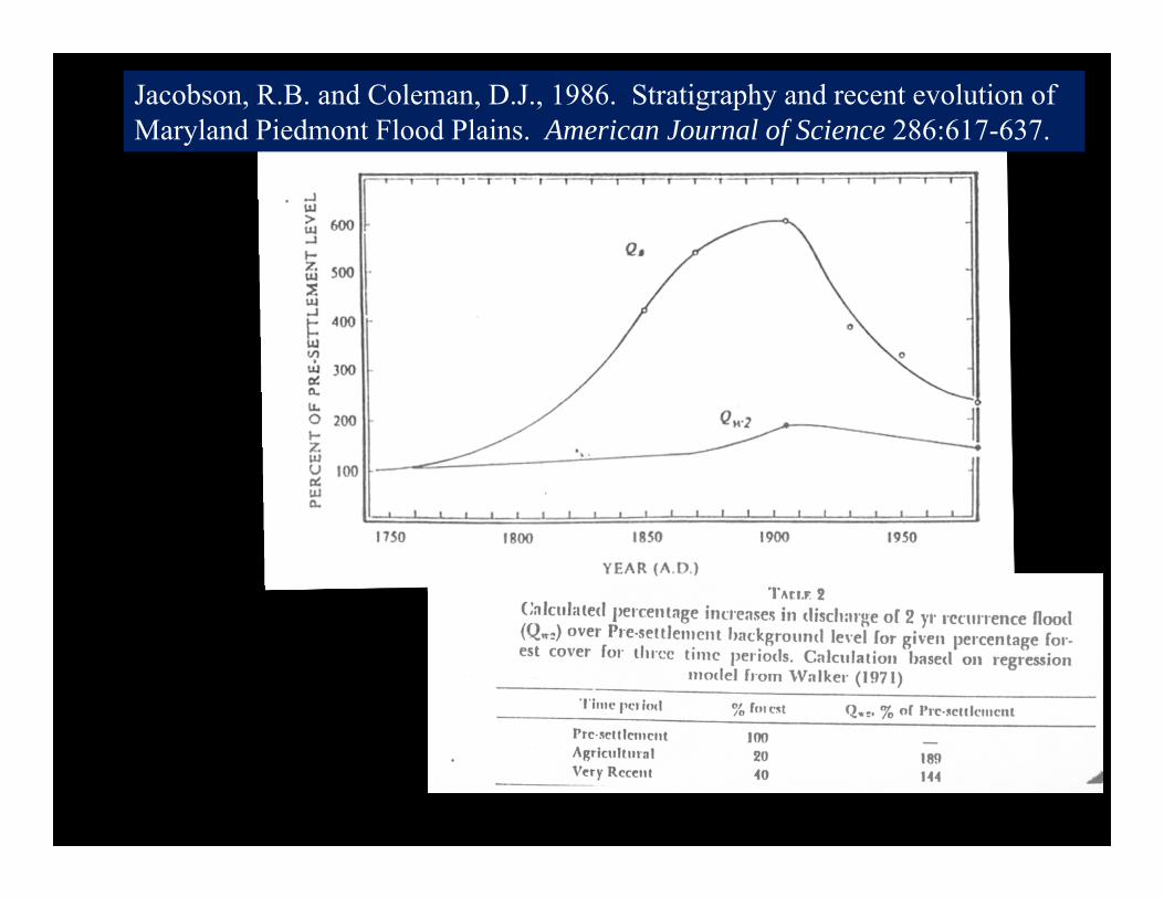
Jacobson, R.B. and Coleman, D.J., 1986. Stratigraphy and recent evolution of Maryland Piedmont Flood Plains. American Journal of Science 286:617-637.

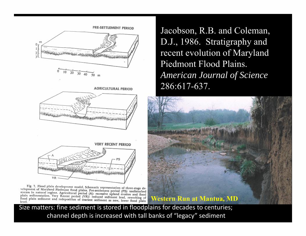
Jacobson, R.B. and Coleman, D.J., 1986. Stratigraphy and recent evolution of Maryland Piedmont Flood Plains. American Journal of Science286:617-637.

Size matters: fine sediment is stored in floodplains for decades to centuries;channel depth is increased with tall banks of “legacy” sediment

Western Run at Mantua, MD

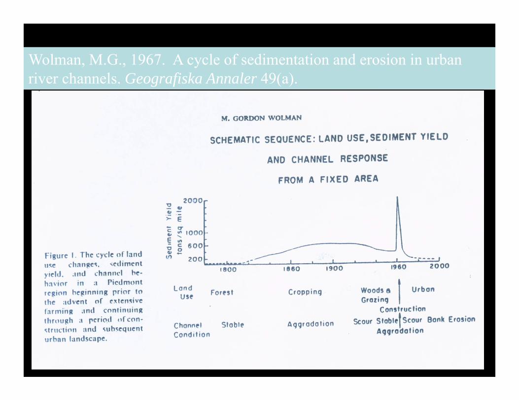
Wolman, M.G., 1967. A cycle of sedimentation and erosion in urban river channels. Geografiska Annaler 49(a).

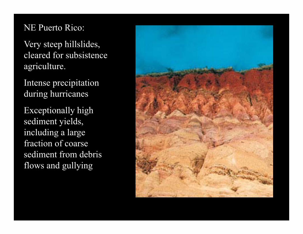
NE Puerto Rico:

Very steep hillslides, cleared for subsistence agriculture.

Intense precipitation during hurricanes

Exceptionally high sediment yields, including a large fraction of coarse sediment from debris flows and gullying

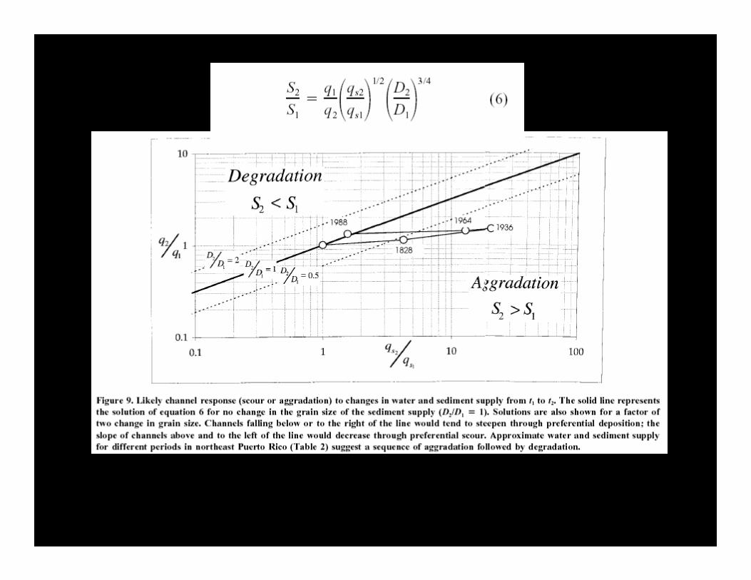
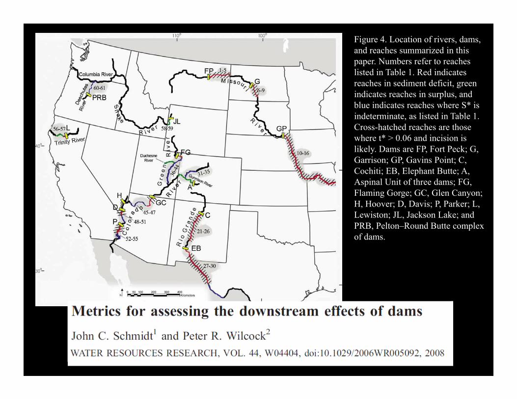
Figure 4. Location of rivers, dams, and reaches summarized in this paper. Numbers refer to reaches listed in Table 1. Red indicates reaches in sediment deficit, green indicates reaches in surplus, and blue indicates reaches where S* is indeterminate, as listed in Table 1. Cross-hatched reaches are those where t* > 0.06 and incision is likely. Dams are FP, Fort Peck; G, Garrison; GP, Gavins Point; C, Cochiti; EB, Elephant Butte; A, Aspinal Unit of three dams; FG, Flaming Gorge; GC, Glen Canyon; H, Hoover; D, Davis; P, Parker; L, Lewiston; JL, Jackson Lake; and PRB, Pelton–Round Butte complex of dams.

Surplus or Deficit?

If Deficit, will channel scour?

Sediment supplyv. transport capacity

Accumulation

Evacuation

Balance indicates

Threshold Channel

Incising, enlarging channel

Aggrading Channel

Sediment Balance Channel Response

(1)Sediment Balance(2)Threshold Evaluation(3)How fast?

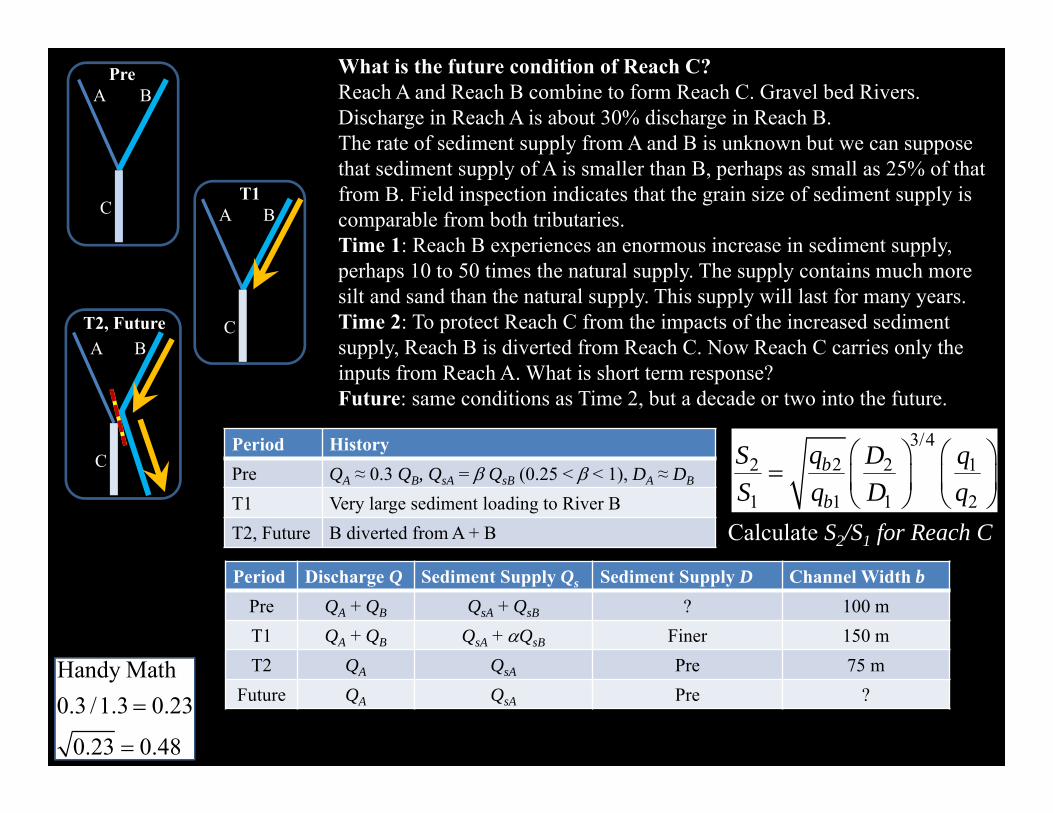
Period Discharge Q Sediment Supply Qs Sediment Supply D Channel Width bPre QA + QB QsA + QsB ? 100 mT1 QA + QB QsA + QsB Finer 150 mT2 QA QsA Pre 75 m

Future QA QsA Pre ?

Period HistoryPre QA ≈ 0.3 QB, QsA = QsB (0.25 < < 1), DA ≈ DB

T1 Very large sediment loading to River BT2, Future B diverted from A + B

What is the future condition of Reach C?Reach A and Reach B combine to form Reach C. Gravel bed Rivers.Discharge in Reach A is about 30% discharge in Reach B. The rate of sediment supply from A and B is unknown but we can suppose that sediment supply of A is smaller than B, perhaps as small as 25% of that from B. Field inspection indicates that the grain size of sediment supply is comparable from both tributaries. Time 1: Reach B experiences an enormous increase in sediment supply, perhaps 10 to 50 times the natural supply. The supply contains much more silt and sand than the natural supply. This supply will last for many years.Time 2: To protect Reach C from the impacts of the increased sediment supply, Reach B is diverted from Reach C. Now Reach C carries only the inputs from Reach A. What is short term response?Future: same conditions as Time 2, but a decade or two into the future.

Handy Math0.3 /1.3 0.23

0.23 0.48

A B

C

Pre

A B

C

T1

A B

C

T2, Future

3/422 2 1

1 1 1 2

b

b

qS D qS q D q

Calculate S2/S1 for Reach C