The effectivity of technological innovationon mitigating the costs of climate changepolicies

C. Kemferta,b, H. Kremersa, and T. Truongc

aDepartment Energy, Transportation, Environment,German Institute for Economic Research,Konigin-Luise-Straße 5,D-14195 Berlin,GermanybHumboldt-Universitat zu Berlin,Spandauer Straße 1,D-10178 Berlin,GermanycSchool of Economics,Faculty of Commerce and Economics,The University of New South Wales,Sydney NSW 2052,Australia

Abstract: Which conditions should technological change in the energy sectors fulfil in order to accomplishcertain emission objectives. Increased emissions cause an increase in mean global temperature which is amajor cause for the changes in mortality and birth rates, and increases health risks. This paper considers anobjective of limiting the rise in mean global temperature to0.1 degree Celcius less than under a Business-as-Usual scenario in2050.

The integrated assessment model WIAGEM explains energy productivity in a production sector as de-termined by the sector’s outlays on research and development in the recent past. The impact of investmentsin research and development on energy productivity depends on an efficiency parameter and an elasticityparameter. The efficiency parameter and elasticity parameter are calibrated in such a way that a temperatureobjective is met. We define two counterfactual scenarios. One scenario limits technological innovation tothe developed regions where the value of the efficiency parameters in these regions are determined suchthat the temperature objective is met. Another scenario extends this scenario to the incorporation of thedeveloping world where the elasticity parameter in these regions are determined such that the temperatureobjective is met.

We use the ’World Integrated Assessment General Equilibrium Model’ (WIAGEM) which combinesan economic general equilibrium model based on the MultiSector-MultiRegional-Trade (MS-MRT) modelwith a climate model and a damage assessment model. WIAGEM is an intertemporal recursive dynamicgeneral equilibrium model with a time horizon. The time span is from1995 until 2050 in time steps of5years.

Keywords: Technological innovation, climate change, learning effects

1 Introduction

Current research on the effects of climate change indicates that the large increase in CO2 emissions

in the period following the industrial age will have major consequences for our societies through

increased health risks and mortality rates, possibly lower birth rates, and changes in productivity

of land. Since many vested interests stand to loose with these changes, serious efforts are being

taken to curb these trends.

Governments are trying to implement new policies that provide society with the incentive to

decrease their emissions. Taxes are imposed on the use of fossil fuels in order to making these

goods relatively expensive to use. International climate agreements such as the Kyoto Protocol

propose to let regions trade in emissions. All these measures mean to put a price on the formerly

free emissions, and this causes extra costs for the production sectors involved.

The success of implementing such climate policies depends crucially on the costs these poli-

cies impose on the production sectors in the economy. The Kyoto Protocol states new options such

as emission permit trading, Joint Implementation, and Clean Development Mechnisms to provide

sectors and regions with the possibilities to obtain their emission reductions in the most cost effec-

tive way possible. On top of this, the international society is putting its hope on the possibilities of

technological innovation in reducing the cost of abatement.

Technological innovation is mainly concentrated on the development of cleaner technologies

or more energy efficient technologies. One can decrease emissions by developing technologies

that emit less such emissions, i.e. they are cleaner, or by developing new technologies that use less

energy, i.e. they are more energy efficient. The effectivity of technological innovation on improv-

ing energy efficiency or obtaining cleaner technologies depends on the effectivity of investments

in improved technologies and on the velocity with which society takes up new technologies.

In this paper, we investigate the effectivity of such technological innovations with respect to

mitigating the effects of climate change on our economy. The economy is represented by an

2

integrated assessment model which couples a computable general equilibrium model with a climate

model. The computable general equilibrium model computes an equilibrium which provides a

certain scenario of emissions in greenhouse gases over time. The climate model uses this scenario

of emissions to compute changes in mean global temperature. The economic model includes the

possibility of technological innovations in the sense that investments in research and development

at certain time will lead to more energy efficient technologies in future periods. The effectivity

of these investments depends on the learning capacity of the economy and on the effectivity of

investments. This paper considers the assumptions that have to be imposed on these parameters

for technological innovation to be effective.

The effectivity of investments in research and development is measured by the extent to which

changes in innovation efforts manage to keep the temperature increase under control at the lowest

costs to the economy. This paper considers assumptions on these parameters which decrease the

mean global temperature due to fossil fuel emissions with0.1 degree Celcius in2050 in compar-

ison to a Business-as-Usual scenario. In this way, we consider the integrated assessment model

from an inverted viewpoint. The assumptions on the innovation parameters that lead to a0.1 de-

crease in mean global temperature are not unique. We consider two combinations that obtain the

required result, and compare them with the business-as-usual scenario in terms of the economic

costs to the economy. One scenario considers only technological innovation in the developed re-

gions where the effectivity of investments in research and development is improved such that our

temperature objective is achieved. The other scenario includes the developing world where the

confrontation with newer, cleaner technologies leads to a quicker acceptance and implementation

of these technologies.

This paper applies the World Integrated Assessment General Equilibrium Model (WIAGEM)

developed in Kemfert (2002). Kemfert (2004) describes the modelling of induced technological

change in more detail and applies it to study the impact of CDM investments. WIAGEM is an

3

integrated assessment model that combines a computable general equilibrium model with a climate

model and a damage assessment model. Section 2 describes the WIAGEM model. In Section 3, we

describe the modelling of technological innovation in WIAGEM. We also describe the assumptions

that we made with respect to the parameters determining the impact of R&D investments and

define the scenarios. Section 4 extensively analyzes and compares the three different scenarios

with respect to the impact on economic development, welfare, and trade. Section 5 draws the

conclusions on this paper.

2 The model

WIAGEM combines an intertemporal general equilibrium model, based on the ’Multi-Sector Multi-

Regional Trade’ (MS-MRT) model, with a climate model, and a damage impact model. For the

MS-MRT model, we refer to (Bernstein et al. 1999a) and Bernstein et al. (1999b). Within the

scope of this paper, we limit our attention to the economic part of WIAGEM with an extension

to the climate model and refer the interested reader to Kemfert (2002) for more information. The

time horizon is50 years, incremented in5-years time steps. It takes1992 as its benchmark year but

it is calibrated using the GTAP4 database complemented with GTAP5 data. The model considers

the period from2000 to 2050.

2.1 Economy

WIAGEM aggregates the world into12 trading regions, which we enumerate in Table 1. Within

this set, we distinguish the subsetAnnexB = {CAN, EU15, JPN, REC, USA} referring to the regions

that signed the Annex B to the Kyoto Protocol.

WIAGEM extends the originally9 production sectors in the MS-MRT model in each region to

15 production sectors. These sectors produce13 tradable goods, which we summarize in Table 2,

4

and another good that refers to investment. The investment good is complemented with another

investment good that refers to research and development activities within the region.

The production factors used in WIAGEM are capital and labour. Physical capital is malleable

but cannot be transferred across sectors. Capital stocks increase over time due to investments from

output produced for domestic sales, and decrease due to depreciation at a constant geometric rate.

The MS-MRT model assumes a two year gestation lag for capital investment and a uniform pattern

of investment within a given10-years period. This means that, ifI(t) is the rate of investment in

periodt, then2I(t) units of capital enter the current capital stock and3I(t) units of capital are

delivered in the next period. The labour force in each period is determined by population growth

and labour-augmenting technical progress. These growth factors are externally given.

For each fossil fuel sector in each region, there exists a resource of this fossil fuel at each time

period. The relation between depletion effects on the supply of oil, gas, and coal, and the actual

supply of these fuels is ignored. The model does not keep a record of the current stock of each fuel

in each time period. This resource therefore represents the demand for this fossil fuel resource in

each time period. This demand is assumed to be constant over time.

Each tradable good in Table 2 is produced in each region by one unique production sector using

a constant returns to scale production technology with the goods in Table 2 as intermediate goods,

and labour and capital as production factors. Under these conditions, the optimal demand for these

inputs are given by the cost minimizing amounts to produce one unit of output times the activity

level. According to Bernstein et al. (1999a), the competitive firms also undertake investments

which arbitrage current investments against future returns. All investments are forward looking

and the producer anticipates the effects of announced policies that are to take effect in the future.

We distinguish between non-energy and electricity production sectors on the one hand and fos-

sil fuel production sectors on the other hand. Output of each non-energy sector and the electricity

sector is decomposed into the intermediate (non-energy) inputs and in a sector specific ’Energy-

5

Value-added’ composite using a Leontief functional form. The non-energy intermediate inputs are

composites of domestically produced goods and their imported equivalents. The ’Energy-Value-

added’ composite is decomposed into an energy composite and a value-added composite using a

Constant Elasticity of Substitution (CES) functional form. WIAGEM decomposes value-added

into its constituents capital and labour also using a CES functional form.

For each fossil fuel production sector, the output good is decomposed into a sector specific fos-

sil fuel resource of this fuel, and a sector specific aggregate good which contains labour, capital,

and this fossil fuel input itself in fixed proportions. The first decomposition uses a CES-function,

while the second layer uses a Leontief production function to represent the fixed proportions.

Final demand in each region is modeled by a representative household, who maximizes its region’s

discounted utility over the model’s time horizon given his income. WIAGEM assumes that the

utility function is of a Constant Intertemporal Elasticity of Substitution (CIES) type. The consumer

obtains income from its endowments of time which it can sell as labour, from his initial endowment

of capital in each production sector, from the rents it obtains on fossil fuel production, and from

tax revenue.

The description of the consumer’s choice between consumption and investment in each period

is derived from growth theoretic models, see Barro and Sala-i-Martin (1995). This model is es-

sentially a so-called Ramsey model. In such models, the consumption-investment decision of an

infinitely living consumer is taken under consideration, where consumption and investment ulti-

mately reach a steady state growth rate which is constant. The model here differs in two important

aspects from the growth theoretic approach: The CGE model considers a finite horizon, and the

CGE model computes a sequence of equilibria which do not imply the existence of a steady state

growth rate in consumption and investment. The solution to the first problem is often to split the

life time of the infinitely living consumer into two parts. The first part consists of the periods under

6

consideration, while the second part considers all remaining time periods. Utility maximization

over the first part starts with an initial endowment of capital in each stock. Utility maximization

over the second part starts with a capital endowment in each stock that would result at the begin-

ning of the next period. The latter stocks are taken from the income of the consumer at the first

period. We have to choose a value for each of these computed capital stocks, which determines

optimal consumption and investment. WIAGEM chooses them by imposing a constant growth

rate on investment in the last period. This condition then becomes an extra condition for the utility

maximizing problem.

Solving the inter-temporal optimization problem results in an optimal consumption plan for

the time span and optimal savings follow indirectly from the remaining income after consumption.

Since we assume the utility function of the consumption household to be homogeneous of degree

one, we use expenditure minimization to obtain the optimal amounts of each good providing one

unit of utility. Total expenditure on consumption equals expenditure per unit of util times the

amount of utils. Total expenditure on consumption plus total expenditure on buying the investment

good equals the consumer’s income in each period.

The model uses a CES function to obtain the aggregate consumption good from a non-energy

composite good and an energy composite. The consumer price index of this composite consump-

tion good is then obtained from the minimum expenditure on the non-energy composite and the

energy composite to obtain one unit of this aggregate consumption good. The non-energy compos-

ite is decomposed into the non-energy goods using a Cobb-Douglas function. The expenditures on

the non-energy goods are composites of domestically produced goods and their imported equiva-

lents. CGE modelers often call such composite goods so-called ’Armington goods’, referring to

Armington (1969).

The consumption and production of non-energy goods contain an energy composite which is de-

7

composed into the output goods of the energy and electricity production sectors. See also Bernstein

et al. (1999b) for a clarification of the energy composite. We use a CES function to decompose

each aggregate into its constituent parts. The energy composite is decomposed into the electricity

good and a fossil fuel aggregate. The electricity goods in these CES functions are again composites

of domestically produced goods of the electricity sector and its imported equivalents. The fossil

composite is decomposed into a coal good and a non-coal composite. The non-coal composite is

decomposed into a gas good and an oil good.

The use of a unit of a fossil fuel will lead to a certain share of emissions in each greenhouse

gas. WIAGEM considers emissions in COa2 nd considers the other greenhouse gases, CH4 and

N2O, in CO2 equivalents. CO2 emissions are computed proportional to the fossil fuel consumption

in each production sector.

Oil is traded internationally as a homogenous good at one price, hence the producer prices of oil in

each region are determined by the world market price. The non-oil fossil fuels as well as the non-

energy goods are represented as ’Armington goods’ to approximate the effects of infrastructure

requirements and high transport costs between some regions. This means that these goods are

composites of its domestically produced and its imported equivalent.

The traded non-oil fossil fuel and non-energy goods are supposed to have different prices de-

pending on whether they are produced for domestic use or for export. WIAGEM uses a Constant

Elasticity of Transformation (CET) function to decompose the output good of these production

sectors. The composite traded non-oil fossil fuel and non-energy goods are decomposed into a

good produced for domestic sales and its equivalents produced for exports using a CET function.

WIAGEM assumes that there is perfect competition on the markets. We define an equilibrium in

this economy as a set of prices and activity levels such that the economy exhibits

8

• market clearing: the activity levels of each production sector clear the market for the par-

ticular output good, while the market for production factors are cleared by the underlying

price.

• zero profits: the price of each tradable good is determined by the minimum cost to produce

one unit of this good.

The market clearing condition depends on whether a tradable good market is considered or a

market for production factors. In the case of a market for tradable goods, the market price of

this good is determined by the marginal cost to produce this good, while the activity level of the

production sector is determined by total demand for this good. The output good of a region’s

production sector is produced to satisfy domestic sales and exported sales. Domestic sales satisfy

the demand for this good as an intermediate good in other domestic production sectors and as

final consumption. Furthermore, we assume that part of domestic sales are meant to represent

investment costs for this production sector.

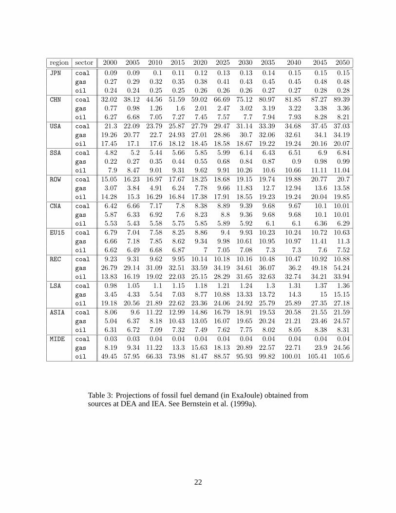
The MS-MRT model’s main characteric is the modelling of energy use and production. This

plays an important role in the model’s calibration where the parameters are determined in such

a way that available data on energy use and production are reproduced in a ’Business-as-Usual’

scenario. The MS-MRT model complements the GTAP4 data with data obtained from sources at

DEA and IEA on fossil fuel demand projections. We have added these data in Table 3.

In any period, a region can be running a trade deficit or a trade surplus, but by the terminal

year, the debt of a region must have been returned to baseline levels. In any infinite horizon model,

this closure rule immediately follows naturally from the budget constraint and prevents the pos-

sibility of an infinite accumulation of debt (the literature refers to a ’no-Ponzi games’ condition).

WIAGEM, as a finite horizon model, approximates this infinite horizon condition by assuming that

there be no net change in foreign indebtedness over the finite horizon. Such closure is consistent

with neoclassical economics (See Bernstein et al. (1999a)).

9

The investments of all production sectors are combined into an aggregate investment good

particular to the region. The activity level of these investment sectors then satisfies demand for

these investment goods. The regional households spend their savings on buying this investment

good. WIAGEM adopts a closure on investment and savings, assuming that there is equality

between total savings of the consumers, i.e. total demand for the investment good, and the supply

of this good by the regional investment sector.

Notice that, in equilibrium, the optimal amount of utils for a representative consumer follows

immediately from equating expenditure per unit of util times the optimal amount of utils to this

consumer’s income. In some sense, the amount of utils of a consumer household plays a role

similar to the activity level of a production sector. It follows from the homogeneity of degree zero

property of the utility functions that the price of a util equals the expenditure to obtain one unit of

it. This util price can be interpreted as a consumer price index.

In the case of a market for production factors, the equilibrium market price arises as the price

clearing the market for this production factor. The capital market is a production sector specific

market. Hence, the price of this sector’s capital good is such that the demand for capital by this

sector is satisfied by the regional endowment of this capital good. The labour market is a regional

market, which makes the wage rate the clearing price between demand for labour by the regional

production sectors and the regional endowment of time spent for labour. Due to the homogeneity

of degree zero in the excess demand and the supply functions in the equilibrium equations, any

positive multiple of an equilibrium price vector will result in an equilibrium. We therefore have to

choose a numeraire good. WIAGEM chooses the wage rate as numeraire.

There will be a gap between producer prices and consumer prices due to possible taxes or

subsidies imposed by the regional government on this good. Similarly, there will be a gap between

export producer price and consumer price due to possible tariffs or export subsidies imposed by a

regional government.

10

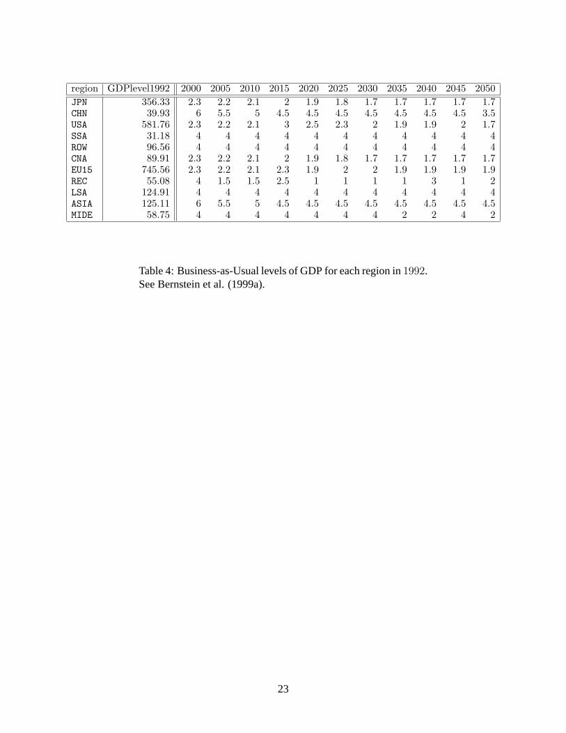
The GTAP4 database provides data for the benchmark year1992, and more data on succeeding

period have to be added in order to be able to calibrate the recursive-dynamic MS-MRT model

over the period between2000 and2050. The data that are available for this objective are often

projections of GDP data for all regions in each period during this time span. These projections

indicate a growth rate for each region which determines growth of resources. Table 4 depicts the

GDP levels for each region in the year1992 and the assumed growth rates as percentages of GDP

in subsequent periods.

2.2 Climate

Global warming is the consequence of the increase in greenhouse gas emissions into the atmo-

sphere. We refer to CO2 emissions, N2O emissions, and CH4 emissions as greenhouse gas emis-

sions. An increase in such emissions results in increased concentrations in the atmosphere, pre-

venting the heat radiated from the earth’s surface to be released. Consequentially, the global tem-

perature on Earth rises to levels where significant damages are expected to occur for the current

human way of life. With respect to damages, we should think of increased risks for human life in

the sense of higher mortality rates, lower birth rates, and health risks. The increase in temperature

also increases sealevels due to a melting of polar ice, causing valuable land to be lost. Higher

precipitation levels may decrease or increase the productivity in land.

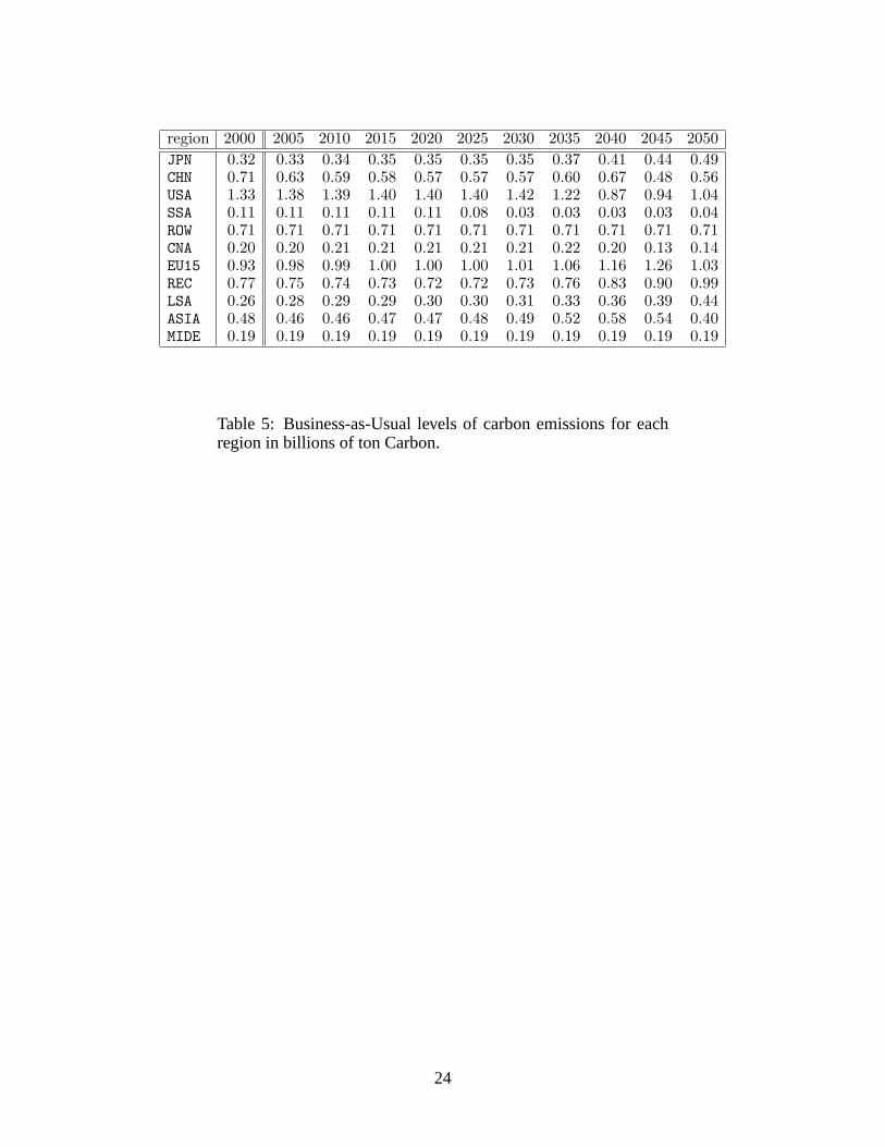
The increase in greenhouse emissions results from human activities as well as natural pro-

cesses. Such human activities require the use of a significant amount of fossil fuels which are seen

to be the major source behind increased CO2 emissions. The MS-MRT model is then calibrated in

such a way that the total emissions for each region as given in Table 5 are generated from the equi-

librium. We obtain total emission in each region by adding the emissions of the regional household

and all production sectors. We then take CO2 emissions as a fixed share of the equilibrium fossil

fuel demand by producers and regional consumer.

11

3 The modelling of technological innovation

A possible action to mitigate the consequences of climate change on our society is seen in the

reduction of energy use in modern production processes through the introduction of more energy

efficient technologies. To be able to obtain such technologies, the computable general equilibrium

model should be extended with the possibility for production sectors to lay aside production for

investments into more energy efficient technologies. We refer to these investments as investments

in research and development.

WIAGEM uses the concept of induced technological change to endogenize technological change.

Induced technological change refers primarily to technological changes following changes in pol-

icy or economic conditions, in contrast to so-called ’autonomous’ technological changes which are

not induced specifically by changes. Induced technological change is implemented via research

and development or via ’learning-by-doing’. WIAGEM implements R&D.

The modelling of induced technological change in CGE models like the one contained in WIA-

GEM often refers to the overview of this material in Buonanno et al. (2000) or earlier, to Nordhaus

(2002). The notion of induced technological change however seems to be first introduced in Hicks

(1932) who noted that ”changes in relative prices production factors such as labour or capital would

spur the development and diffusion of new technologies in order to economize on the usage of the

more expensive productionn sector”. As for details on how to model induced technological change

in what we call ’top-down’ models as WIAGEM, we refer to Goulder and Mathai (2000) and to

Goulder and Schneider (1999).

The total amount of R&D investments results, in due time, in a more efficient use of energy in

the production and household sectors of the host regions. It is convenient to follow regular prac-

tice in modern endogenous growth theory here, when we want to model improvements in efficiency

into the CGE model. We refer to details on endogenous growth theory in Barro and Sala-i-Martin

(1995). This literature introduces so-called efficiency units to introduce endogenously determined

12

changes in technology into the model. In our model, this means that we have to consider the

input or consumption of the energy composite in efficiency units. Kemfert (2002) takes such an

approach, where investments in research and development are related to changes in the AEEI pa-

rameter associated with energy use. We follow this approach by stating a relation between total

investments in research and development and changes in this AEEI parameter within the produc-

tion and household sectors. The parameter∆AEEI(r, t) for regionr refers to the change in the

AEEI parameter following energy efficiency improving investments in research and development

in regionr. We use the following constant demand elasticity functional form

∆AEEI(r, t) = δt,r · ∆R&D(r, t)εr , (1)

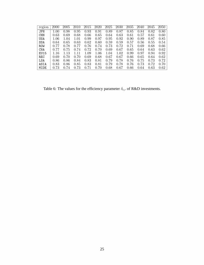
for this relationship. The parameterδt,r can be seen as an efficiency parameter while the parameter

εr can be seen as the elasticity parameter in equation (1). A relatively high value of the efficiency

parameterδt,r indicates a relatively high influence of the investments on the energy efficiency. An

increase in investments by one percent, causes an increase in energy efficiency byεr. A relatively

high value ofεr indicates a high effectivity of investments in regionr on energy use efficiency.

WIAGEM takes the elasticity parameterεr equal to0.2 for each region, while Table 6 presents the

value of the efficiency parameter in each period in each region.

Business-as-Usual. WIAGEM follows the MS-MRT model by calibrating the economic sub-

model on the GTAP4 database. This calibration provides values for the share parameters of the

model in the year of calibration,1992. For the subsequent time periods, these share parameters

are updated in such a way that the MS-MRT model reproduces the scenarios predicted by other

models or data from scientific institutions. The MS-MRT model is calibrated to the development

of GDP (Table 4), fossil fuel demand (Table 3), and emission levels (Table 5) over time.

13

The international society expects a lot from the possibilities of technological innovation in reducing

the costs of emission reduction. But, whether technological innovation manages to reduce the costs

of emissions on our society and meanwhile enables society to reach the goal of limiting a global

temperature increase to only0.1 degree less than the ’Business-as-Usual’ in2050 depends among

others on the efficiency with which new technologies can be implemented into the economy and

the speed of learning in this economy. We define two possible scenarios to study the impact of

different values forδt,r andεr on these goals. In the ”Business-as-Usual” scenario, mean global

temperature is assumed to rise according to Table 7. We can conclude from the latter table that, in

2050 mean global temperature has risen with3.809 degrees Celcius compared to the benchmark in

1992.

Developed regions. This scenario assumes that only the developed regions are actively engaged

in technological innovation. Technological innovations in the developed world lead to improve-

ments in the efficiency parameterδt,r and the elasticity parameterεr for all developed regionsr.

We assume that continuous improvements and communication results in a technological innova-

tion that improves these parameters with the same percentages for each developed regionr. This

means that we have to determine a valueδ such that the efficiency parametersδt,r(1 + δ) for all

developed regionsr manages to keep the global temperature rise limited to3.709 degree Celcius

in 2050. Computational experiments on the value ofδ indicate a value of0.325. We do not assume

any effects on the developing regions to take place, henceε = 0 in this scenario.

Developing regions. This scenario extends the ’Developed regions’ scenario to an involvement

of the developing regions. We assume that technological innovation in the developing world takes

place through a learning effect. The developing regions are assumed to learn from the technology

in the developed world causing an improvement of the elasticity parameterεr for all developing

regionsr. This means that we have to determine a valueε such that the learning elasticityεr(1+ ε)

14

for all developing regionsr manages to keep the global temperature rise limited to3.709 degree

Celcius in2050. The possibility for the developed regions to obtain part of their emission re-

ductions in the developing regions would indicate that the valueδ referred to in the ’Developed

regions’ scenario can be closer to zero or even dissappear causing lower costs to the developed

regions.

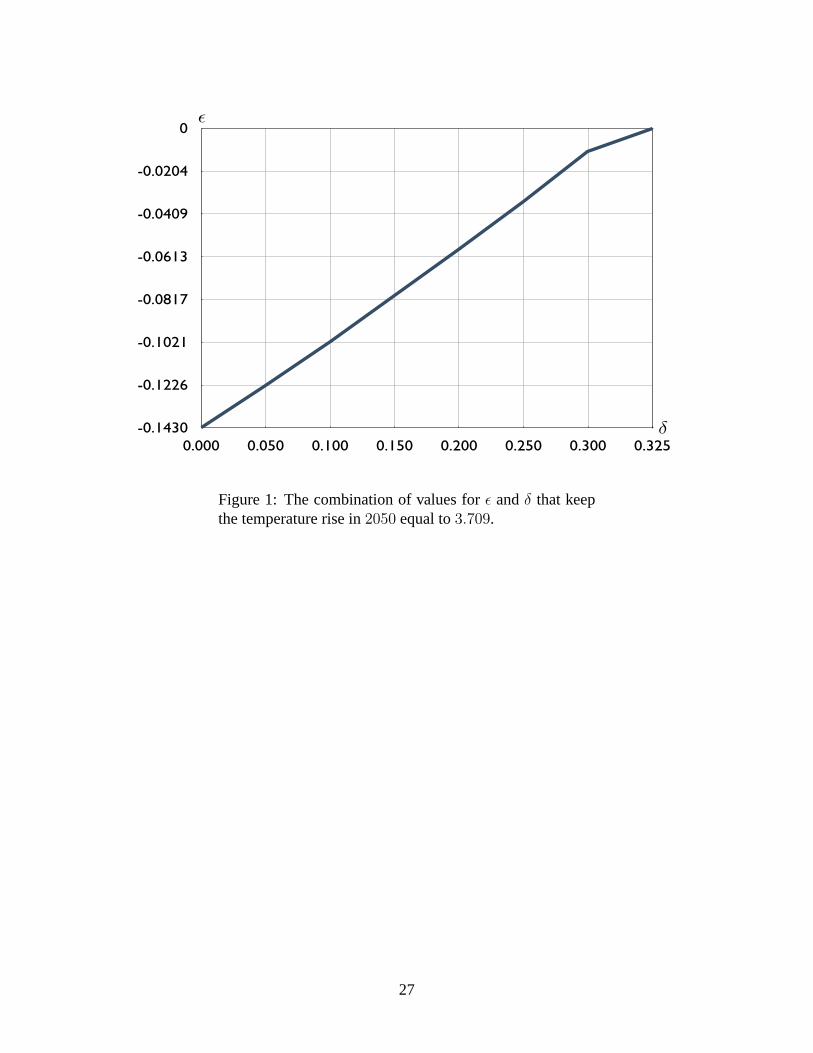
In Figure 1, we depict the combinations of values forε andδ that will result in a temperature

increase of3.709 in 2050, i.e. a limitation of the temperature increase with0.1 degrees less than

the BaU situation. In this figure,δ represents the change in efficiency necessary in the developed

regions andε represents the change in learning capacity necessary in the developing world to

allow an efficiency increase equal toδ in the developed world. We assume an extreme case to be

occurring here. Let us takeε = −0.1430. Figure 1 then indicates that no efficiency gain must be

taken in the developed world, henceδ = 0.

4 Simulations

In this section, we calculate the costs of the scenarios that we defined in the previous section. We

refer to the opportunity costs of the Annex I regions as given by their marginal costs of emissions

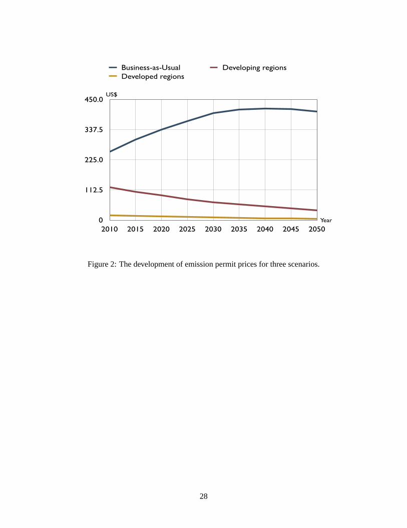
which, in our model equals the price of emission permits on the market. Figure 2 illustrates the

development of the value of the permit price on the market for emission permits under three dif-

ferent scenarios. We distinguish the Business-as-Usual scenario to which also the model has been

calibrated. This scenario corresponds to a value ofδ and ofε equal to zero. In the first counterfac-

tual scenario defined in the previous section, the ’Developed regions’ scenario, we ask what kind

of change in efficiency in the developed regions only is necessary to reduce the temperature rise

with 0.1 degrees Celcius compared to the Business-as-Usual. We computed a value forδ equal

to 0.325, under the assumption that no learning takes place in the developing regions. Hence, the

15

’Developed regions’ scenario refers to a value ofδ equal to0.325 and a value of0 of ε. In the

second counterfactual scenario, we allow the developed regions to export their modern technology

to the developing regions. In our scenarios, this results in a change in the learning capacity of

the developing regions corresponding to lower values for the ’learning elasticity’εr for develop-

ing regionsr. In Figure 2, we illustrate the extreme case where the temperature change can only

be reached by extra learning capacity in the developing regions, i.e. this line corresponds to the

situation whereδ = 0 andε = −0.143.

In Figure 2, we see that improvements in the efficiency of R&D investments decreases the price

of emission permits. Equation (1) indicates that improved efficiency results in a higher value of

the AEEI parameter for the production sectors in the developed world. This improved efficiency in

energy use indicates a lower energy use, thereby less emissions, hence less demand for emission

permits per unit of output. The decreased demand lowers the price for emission permits necessary

to clear the underlying market.

The other scenario, the ’Developing countries’ scenario, is depicted in one of its extremes, by

assumingδ = 0. If no efficiency gain takes place in the Annex I regions, and the reduction in

temperature increase can only be obtained with a decrease in the elasticityεr for the developing

regionsr, then we see that the price of emission permits decreases significantly with respect to the

Business-as-Usual scenario but not as much as in the previously addressed scenario. A decrease

in this elasticity implies that the AEEI factor in the developing regions’ production technologies

increases significantly. The production sectors in these regions therefore need less investments

in R&D to obtain the same effect on the AEEI as under the Business-as-Usual scenario. On the

other hand, the price of the energy composite in these technologies will be decreased, causing

energy intensive products to become relatively cheap in the developing world. Here, demand will

be shifting from the now relatively expensive imports from the developed world to the cheaper

domestically produced goods. The Annex I regions then need to produce less of these energy

16

intensive goods than before, with lower emissions as a consequence. This decreases demand for

the emission permits required for production hence leading to a lower permit price to clear the

market. This decrease is less than in the ’developed regions’ scenario since it is caused by an

indirect effect.

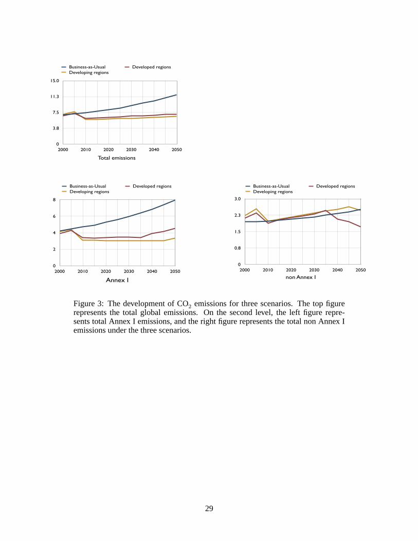
In Figure 3, we illustrated the consequences of implementing our scenarios on total emissions, on

the emissions of the Annex I regions, and the emissions of the non Annex I regions. This leads

to three figures, each one corresponding to one of the scenarios defined in the previous section.

The top figure depicts the total global emissions. These emissions contain total emissions for the

Annex I regions, depicted in the left figure, and the total emissions for the non Annex I regions,

depicted in the right figure on the lower level of Figure 3.

The figure referring to the emissions of the Annex I regions shows that both counterfactuals

significantly reduce emissions as expected, from2005 on. Since WIAGEM is an intertemporal

model, producers and consumers take account of the future in their decisions, and this sudden

decrease in emissions in2005 is in anticipation of the increased prices for emissions in the near

future. Notice also that emissions rise at the end of the total period, towards2050, since WIAGEM

considers only a finite time and, as described in Section 2, the last period also takes account of

what happens after2050. The ’Developing regions’ scenario also has more influence on Annex

I emissions than the ’Developed regions’ scenario. The reduction of imports of energy intensive

goods from the Annex I regions obviously reduces emissions here to a large extent.

The figure referring to the emissions of the non Annex I regions provides a mixed view. Emis-

sions of the non Annex I regions lie above the Business-as-Usual levels for a long time, but on the

longer term emissions under this counterfactual will decrease sufficiently. The ’developed regions’

scenario works out more efficiently on emissions in non Annex I regions than the ’developed re-

gions’ scenario. Total emissions, depicted in the top figure, contains all influences on the emissions

of Annex I and non Annex I regions.

17

5 Conclusions

The international society has great expectations about the possibilities of technological change

in reducing the costs of implementing climate change policies on the economies of the developed

world. In this paper, we investigated the conditions that should be imposed on technological change

in order to limit the increase in mean global temperature in2050 to 0.1 degree less than under

a Business-as-Usual scenario. We use the ’World Integrated Assessment General Equilibrium

Model’ (WIAGEM), an integrated assessment model that combines an intertemporal computable

general equilibrium model with a climate model. WIAGEM endogenizes technological change into

the CGE model in the form of induced technological change where investments in research and

development result in an improved AEEI parameter attached to the use of energy in the production

sectors. The relation between the change in the AEEI parameter and the investments in research

and development depends on an efficiency parameter and a ’learning’ elasticity, the latter elasticity

giving some indication on how easy new technological knowledge can be assimilated into the

production technologies of an economy.

We defined two counterfactual scenarios to be compared to the Business-as-Usual to which WI-

AGEM has been calibrated. In one counterfactual, we only let changes in the efficiency parameter

of the developed regions be responsible for improvements in the AEEI parameters. No contribu-

tion is expected from the developing world. We referred to this counterfactual as the ’Developed

regions’ counterfactual. We then take another extreme, by defining a counterfactual scenario ’De-

veloping regions’ where we only let changes in the ’learning elasticity’ of the developing regions

be responsible for changes in the AEEI parameters. Both scenarios have a significant impact on the

price of emission permits on the Annex I permit trading market. This price, in our model, equals

the marginal cost of emissions in the regions that participate on this market. Hence, technological

change significantly reduces these costs. As for total global emission, even under these conditions,

technological change following investments in research and development, is not able to curb emis-

18

sions. Emissions will be generally lower as compared to the Business-as-Usual scenario, but they

still increase over time, indicating only a postponement of the consequences of climate change to

a later date.

References

Armington, P. (1969). A theory of demand for products distinguished by place of production.IMFStaff Papers 16, 159–178.

Barro, R. and X. Sala-i-Martin (1995).Economic Growth. New York: McGraw-Hill.

Bernstein, P., W. Montgomery, and T. Rutherford (1999a). Global impacts of the Kyoto agreement:results from the MS-MRT model.Resource and Energy Economics 21, 375–413.

Bernstein, P., W. Montgomery, T. Rutherford, and G. Yang (1999b). Effects of restrictions oninternational permit trading: the MS-MRT model.The Energy Journal, 221–256. KyotoSpecial Issue.

Buonanno, P., C. Carraro, and M. Galeotti (2000). Endogenous induced technical change and thecosts of Kyoto.Resource and Energy Economics 25(1), 11–34.

Goulder, L. and K. Mathai (2000). Optimal CO2 abatement in the presence of induced technolog-ical change.Journal of Environmental Economics and Management 39(1), 1–38.

Goulder, L. and S. Schneider (1999). Induced technological change and the attractiveness of CO2

abatement policies.Resource and Energy Economics 21(3-4), 211–253.

Hicks, J. (1932).The Theory of Wages. London: MacMillan.

Kemfert, C. (2002). An Integrated Assessment model of economy-energy-climate− The modelWIAGEM. Integrated Assessment 3, 281–298.

Kemfert, C. (2004). Induced technological change in a multi-regional, multi-sectoral integratedassessment model (WIAGEM). Impact assessment of climate policy strategies. Discussionpaper 435, Deutsches Institut fur Wirtschaftsforschung (DIW), Berlin.

Nordhaus, W. (2002). Modelling induced innovation in climate change policy. In A. Grubler,N. Nakicenovic, and W. Nordhaus (Eds.),Technological change and the environment, Wash-ington D.C. and Laxenburg, pp. 182–209. Resources for the future (RFF) and InternationalInstitute for Applied Systems Analysis (IIASA).

19

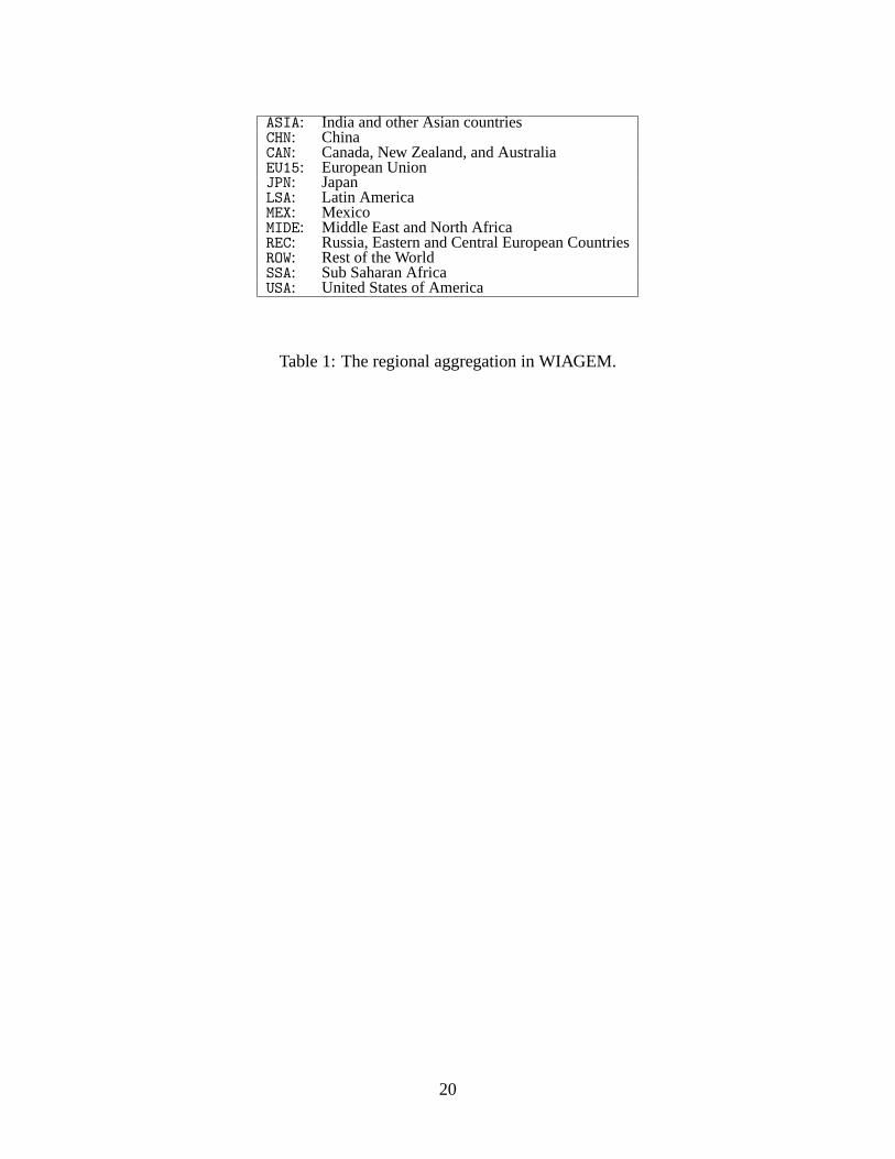
ASIA: India and other Asian countriesCHN: ChinaCAN: Canada, New Zealand, and AustraliaEU15: European UnionJPN: JapanLSA: Latin AmericaMEX: MexicoMIDE: Middle East and North AfricaREC: Russia, Eastern and Central European CountriesROW: Rest of the WorldSSA: Sub Saharan AfricaUSA: United States of America

Table 1: The regional aggregation in WIAGEM.

20

AgricultureCoalChemical rubber and plasticsCrude oilElectricityNatural gasNonferrous metalsNonmetal mineral productsPetroleum and coal productsOther manufactures and servicesIron and steelPulp and paperTransport industries

Table 2: The sectoral aggregation of traded goods in WIAGEM.

21

region sector 2000 2005 2010 2015 2020 2025 2030 2035 2040 2045 2050JPN coal 0.09 0.09 0.1 0.11 0.12 0.13 0.13 0.14 0.15 0.15 0.15

gas 0.27 0.29 0.32 0.35 0.38 0.41 0.43 0.45 0.45 0.48 0.48oil 0.24 0.24 0.25 0.25 0.26 0.26 0.26 0.27 0.27 0.28 0.28

CHN coal 32.02 38.12 44.56 51.59 59.02 66.69 75.12 80.97 81.85 87.27 89.39gas 0.77 0.98 1.26 1.6 2.01 2.47 3.02 3.19 3.22 3.38 3.36oil 6.27 6.68 7.05 7.27 7.45 7.57 7.7 7.94 7.93 8.28 8.21

USA coal 21.3 22.09 23.79 25.87 27.79 29.47 31.14 33.39 34.68 37.45 37.03gas 19.26 20.77 22.7 24.93 27.01 28.86 30.7 32.06 32.61 34.1 34.19oil 17.45 17.1 17.6 18.12 18.45 18.58 18.67 19.22 19.24 20.16 20.07

SSA coal 4.82 5.2 5.44 5.66 5.85 5.99 6.14 6.43 6.51 6.9 6.84gas 0.22 0.27 0.35 0.44 0.55 0.68 0.84 0.87 0.9 0.98 0.99oil 7.9 8.47 9.01 9.31 9.62 9.91 10.26 10.6 10.66 11.11 11.04

ROW coal 15.05 16.23 16.97 17.67 18.25 18.68 19.15 19.74 19.88 20.77 20.7gas 3.07 3.84 4.91 6.24 7.78 9.66 11.83 12.7 12.94 13.6 13.58oil 14.28 15.3 16.29 16.84 17.38 17.91 18.55 19.23 19.24 20.04 19.85

CNA coal 6.42 6.66 7.17 7.8 8.38 8.89 9.39 9.68 9.67 10.1 10.01gas 5.87 6.33 6.92 7.6 8.23 8.8 9.36 9.68 9.68 10.1 10.01oil 5.53 5.43 5.58 5.75 5.85 5.89 5.92 6.1 6.1 6.36 6.29

EU15 coal 6.79 7.04 7.58 8.25 8.86 9.4 9.93 10.23 10.24 10.72 10.63gas 6.66 7.18 7.85 8.62 9.34 9.98 10.61 10.95 10.97 11.41 11.3oil 6.62 6.49 6.68 6.87 7 7.05 7.08 7.3 7.3 7.6 7.52

REC coal 9.23 9.31 9.62 9.95 10.14 10.18 10.16 10.48 10.47 10.92 10.88gas 26.79 29.14 31.09 32.51 33.59 34.19 34.61 36.07 36.2 49.18 54.24oil 13.83 16.19 19.02 22.03 25.15 28.29 31.65 32.63 32.74 34.21 33.94

LSA coal 0.98 1.05 1.1 1.15 1.18 1.21 1.24 1.3 1.31 1.37 1.36gas 3.45 4.33 5.54 7.03 8.77 10.88 13.33 13.72 14.3 15 15.15oil 19.18 20.56 21.89 22.62 23.36 24.06 24.92 25.79 25.89 27.35 27.18

ASIA coal 8.06 9.6 11.22 12.99 14.86 16.79 18.91 19.53 20.58 21.55 21.59gas 5.04 6.37 8.18 10.43 13.05 16.07 19.65 20.24 21.21 23.46 24.57oil 6.31 6.72 7.09 7.32 7.49 7.62 7.75 8.02 8.05 8.38 8.31

MIDE coal 0.03 0.03 0.04 0.04 0.04 0.04 0.04 0.04 0.04 0.04 0.04gas 8.19 9.34 11.22 13.3 15.63 18.13 20.89 22.57 22.71 23.9 24.56oil 49.45 57.95 66.33 73.98 81.47 88.57 95.93 99.82 100.01 105.41 105.6

Table 3: Projections of fossil fuel demand (in ExaJoule) obtained fromsources at DEA and IEA. See Bernstein et al. (1999a).

22

region GDPlevel1992 2000 2005 2010 2015 2020 2025 2030 2035 2040 2045 2050JPN 356.33 2.3 2.2 2.1 2 1.9 1.8 1.7 1.7 1.7 1.7 1.7CHN 39.93 6 5.5 5 4.5 4.5 4.5 4.5 4.5 4.5 4.5 3.5USA 581.76 2.3 2.2 2.1 3 2.5 2.3 2 1.9 1.9 2 1.7SSA 31.18 4 4 4 4 4 4 4 4 4 4 4ROW 96.56 4 4 4 4 4 4 4 4 4 4 4CNA 89.91 2.3 2.2 2.1 2 1.9 1.8 1.7 1.7 1.7 1.7 1.7EU15 745.56 2.3 2.2 2.1 2.3 1.9 2 2 1.9 1.9 1.9 1.9REC 55.08 4 1.5 1.5 2.5 1 1 1 1 3 1 2LSA 124.91 4 4 4 4 4 4 4 4 4 4 4ASIA 125.11 6 5.5 5 4.5 4.5 4.5 4.5 4.5 4.5 4.5 4.5MIDE 58.75 4 4 4 4 4 4 4 2 2 4 2

Table 4: Business-as-Usual levels of GDP for each region in1992.See Bernstein et al. (1999a).

23

region 2000 2005 2010 2015 2020 2025 2030 2035 2040 2045 2050JPN 0.32 0.33 0.34 0.35 0.35 0.35 0.35 0.37 0.41 0.44 0.49CHN 0.71 0.63 0.59 0.58 0.57 0.57 0.57 0.60 0.67 0.48 0.56USA 1.33 1.38 1.39 1.40 1.40 1.40 1.42 1.22 0.87 0.94 1.04SSA 0.11 0.11 0.11 0.11 0.11 0.08 0.03 0.03 0.03 0.03 0.04ROW 0.71 0.71 0.71 0.71 0.71 0.71 0.71 0.71 0.71 0.71 0.71CNA 0.20 0.20 0.21 0.21 0.21 0.21 0.21 0.22 0.20 0.13 0.14EU15 0.93 0.98 0.99 1.00 1.00 1.00 1.01 1.06 1.16 1.26 1.03REC 0.77 0.75 0.74 0.73 0.72 0.72 0.73 0.76 0.83 0.90 0.99LSA 0.26 0.28 0.29 0.29 0.30 0.30 0.31 0.33 0.36 0.39 0.44ASIA 0.48 0.46 0.46 0.47 0.47 0.48 0.49 0.52 0.58 0.54 0.40MIDE 0.19 0.19 0.19 0.19 0.19 0.19 0.19 0.19 0.19 0.19 0.19

Table 5: Business-as-Usual levels of carbon emissions for eachregion in billions of ton Carbon.

24

region 2000 2005 2010 2015 2020 2025 2030 2035 2040 2045 2050JPN 1.00 0.98 0.95 0.93 0.91 0.89 0.87 0.85 0.84 0.82 0.80CHN 0.63 0.69 0.68 0.66 0.65 0.64 0.63 0.61 0.57 0.61 0.60USA 1.06 1.04 1.01 0.99 0.97 0.95 0.92 0.90 0.89 0.87 0.85SSA 0.64 0.65 0.63 0.62 0.60 0.59 0.59 0.57 0.56 0.55 0.54ROW 0.77 0.78 0.77 0.76 0.74 0.73 0.72 0.71 0.69 0.68 0.66CNA 0.77 0.75 0.74 0.72 0.70 0.69 0.67 0.65 0.64 0.63 0.62EU15 1.16 1.13 1.11 1.09 1.06 1.04 1.02 0.99 0.97 0.94 0.92REC 0.69 0.70 0.70 0.69 0.68 0.67 0.67 0.66 0.65 0.64 0.62LSA 0.86 0.86 0.84 0.83 0.81 0.79 0.78 0.76 0.75 0.73 0.72ASIA 0.83 0.86 0.85 0.83 0.81 0.79 0.78 0.76 0.73 0.72 0.70MIDE 0.73 0.74 0.73 0.71 0.70 0.68 0.67 0.66 0.64 0.63 0.62

Table 6: The values for the efficiency parameterδt,r of R&D investments.

25

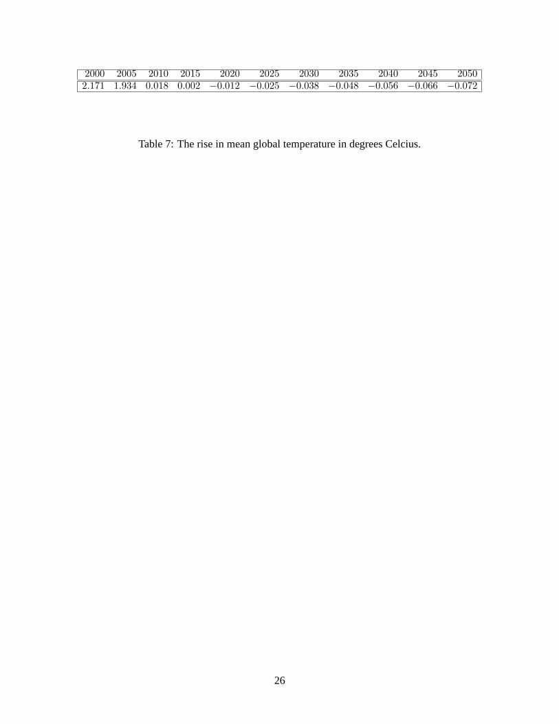
2000 2005 2010 2015 2020 2025 2030 2035 2040 2045 20502.171 1.934 0.018 0.002 −0.012 −0.025 −0.038 −0.048 −0.056 −0.066 −0.072

Table 7: The rise in mean global temperature in degrees Celcius.

26

0.000 0.050 0.100 0.150 0.200 0.250 0.300 0.325-0.1430

-0.1226

-0.1021

-0.0817

-0.0613

-0.0409

-0.0204

0

ε

δ

Figure 1: The combination of values forε andδ that keepthe temperature rise in2050 equal to3.709.

27

2010 2015 2020 2025 2030 2035 2040 2045 20500

112.5

225.0

337.5

450.0

Business-as-UsualDeveloped regions

Developing regions

US$

Year

Figure 2: The development of emission permit prices for three scenarios.

28

2000 2010 2020 2030 2040 20500

3.8

7.5

11.3

15.0

Business-as-UsualDeveloping regions

Developed regions

Total emissions

2000 2010 2020 2030 2040 20500

2

4

6

8

Business-as-UsualDeveloping regions

Developed regions

Annex I

2000 2010 2020 2030 2040 20500

0.8

1.5

2.3

3.0

Business-as-UsualDeveloping regions

Developed regions

non Annex I

Figure 3: The development of CO2 emissions for three scenarios. The top figurerepresents the total global emissions. On the second level, the left figure repre-sents total Annex I emissions, and the right figure represents the total non Annex Iemissions under the three scenarios.

29