the effect of shadow education vouchers after the great ... · 1 rieti discussion paper series...

DPRIETI Discussion Paper Series 18-E-031

The Effect of Shadow Education Vouchersafter the Great East Japan Earthquake:

Evidence from regression discontinuity design

KOBAYASHI YoheiRIETI

The Research Institute of Economy, Trade and Industryhttps://www.rieti.go.jp/en/

https://www.rieti.go.jp/en/index.html

1

RIETI Discussion Paper Series 18-E-031

May 2018

The Effect of Shadow Education Vouchers

after the Great East Japan Earthquake:

Evidence from regression discontinuity design*

KOBAYASHI Yohei

Research Institute of Economy, Trade and Industry

Mitsubishi UFJ Research and Consulting†

Abstract

Shadow education vouchers, which beneficiaries flexibly use for any pre-

registered institutions such as cram schools and one-to-one tutoring, might be

an effective method to support disadvantaged children. In this paper, we

estimate empirically the effects of shadow education vouchers provided in the

area affected by the Great East Japan Earthquake on mainly cognitive skills by

utilizing regression discontinuity design. Our results show a positive impact

on academic achievements and study hours during holidays. In addition, the

impact is much larger for children living in poverty.

Keywords: Shadow education voucher, Cognitive skill, Child poverty,

Regression Discontinuity design, Randomization inference

JEL classification: I24, I26, I38, C21

RIETI Discussion Papers Series aims at widely disseminating research results in the form of

professional papers, thereby stimulating lively discussion. The views expressed in the papers are

solely those of the author(s), and neither represent those of the organization to which the author(s)

belong(s) nor the Research Institute of Economy, Trade and Industry.

* This study is conducted as a part of the project “Reform of Labor Market Institutions” undertaken at the

Research Institute of Economy, Trade and Industry (RIETI). The author is grateful to Michihito Ando,

Yusuke Imai, Makoto Kato, Yuki Kitashita, Masayuki Morikawa, Makiko Nakamuro, Suzuko Noda,

Kotaro Tsuru, Makoto Yano, and Discussion Paper seminar participants at RIETI for their valuable

comments and supports. The views and opinions expressed here are those of the author and not

necessarily those of the Chance for Children or any of its stakeholders. The author is solely responsible

for any remaining errors. † E-mail:[email protected]

2

1 Introduction

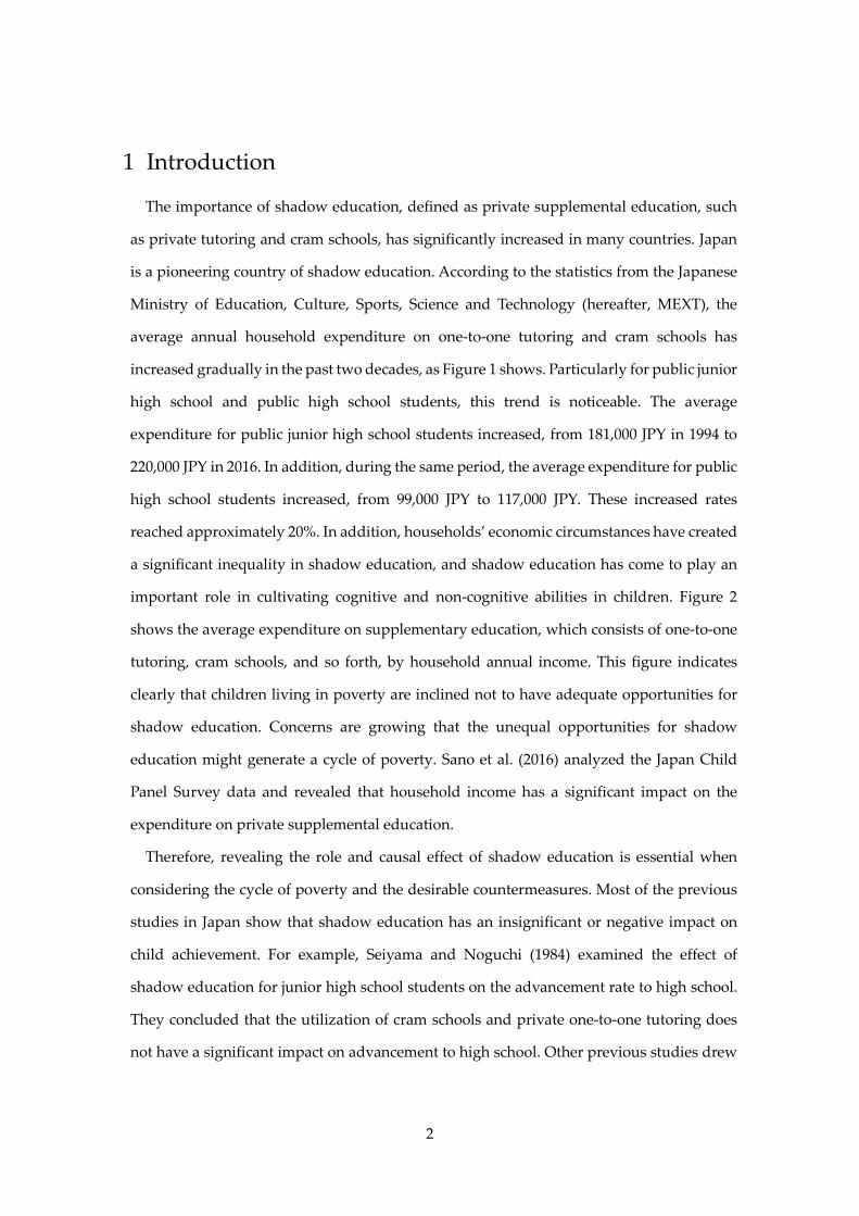
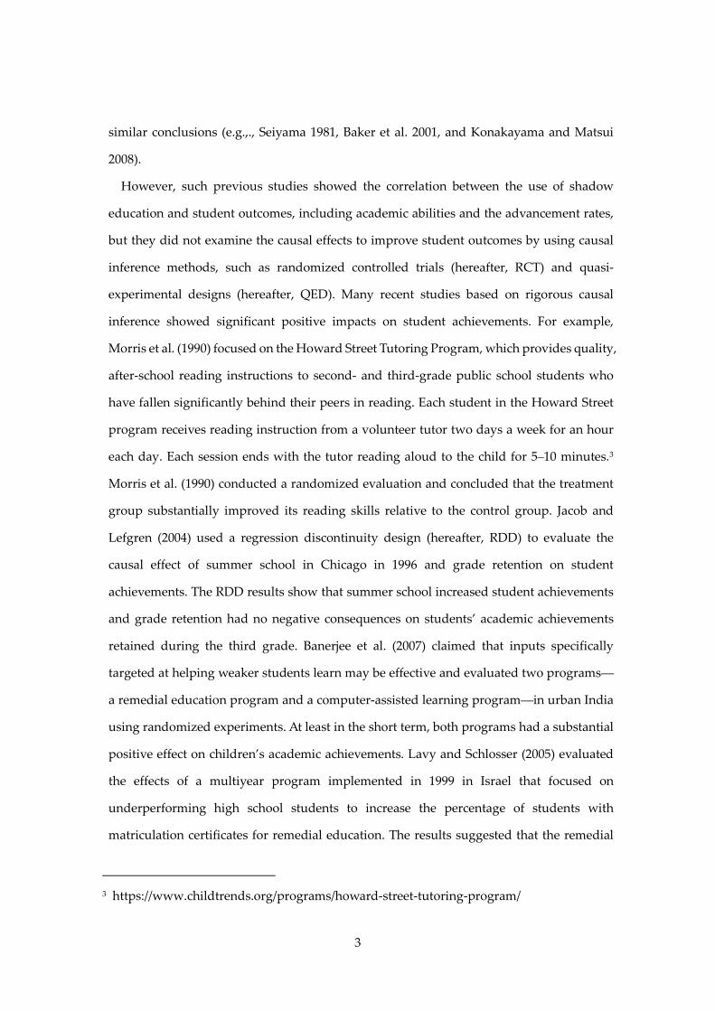
The importance of shadow education, defined as private supplemental education, such

as private tutoring and cram schools, has significantly increased in many countries. Japan

is a pioneering country of shadow education. According to the statistics from the Japanese

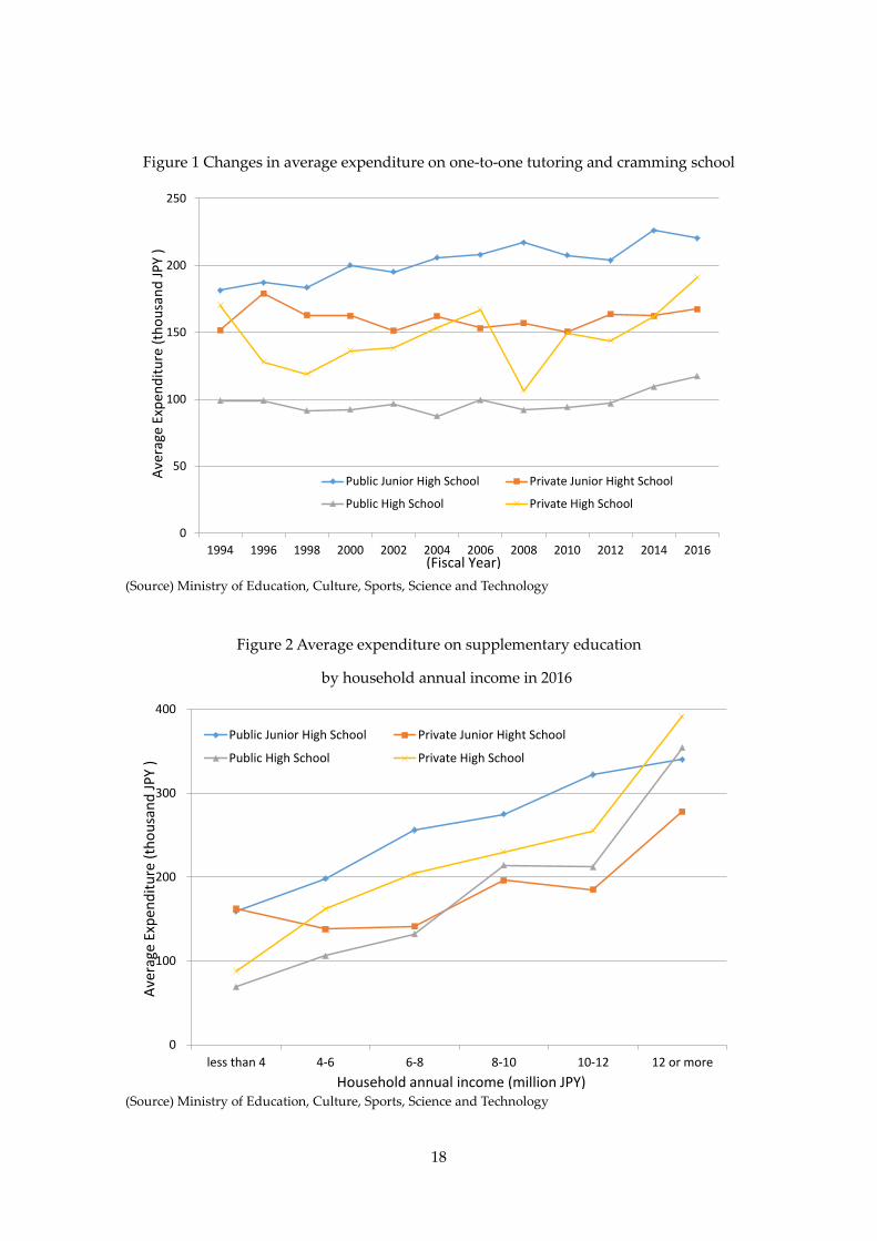
Ministry of Education, Culture, Sports, Science and Technology (hereafter, MEXT), the

average annual household expenditure on one-to-one tutoring and cram schools has

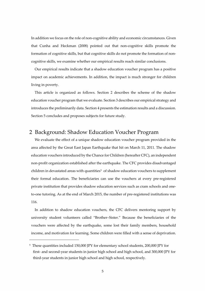
increased gradually in the past two decades, as Figure 1 shows. Particularly for public junior

high school and public high school students, this trend is noticeable. The average

expenditure for public junior high school students increased, from 181,000 JPY in 1994 to

220,000 JPY in 2016. In addition, during the same period, the average expenditure for public

high school students increased, from 99,000 JPY to 117,000 JPY. These increased rates

reached approximately 20%. In addition, households’ economic circumstances have created

a significant inequality in shadow education, and shadow education has come to play an

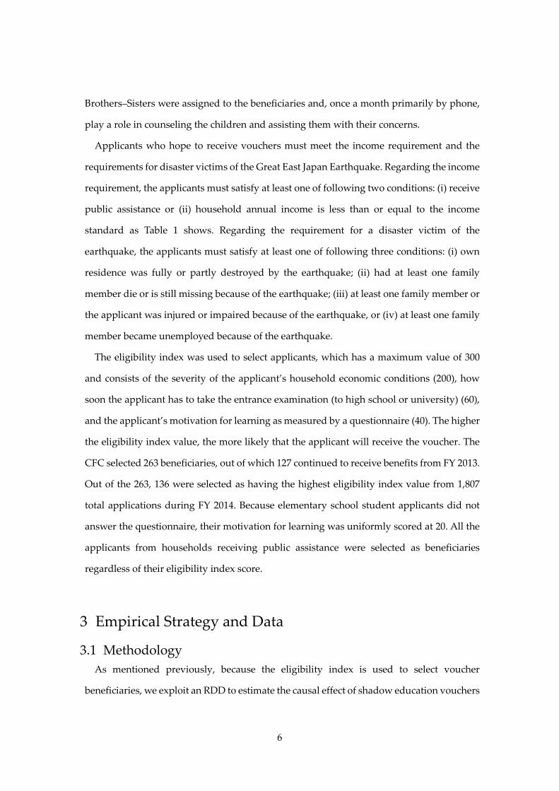
important role in cultivating cognitive and non-cognitive abilities in children. Figure 2

shows the average expenditure on supplementary education, which consists of one-to-one

tutoring, cram schools, and so forth, by household annual income. This figure indicates

clearly that children living in poverty are inclined not to have adequate opportunities for

shadow education. Concerns are growing that the unequal opportunities for shadow

education might generate a cycle of poverty. Sano et al. (2016) analyzed the Japan Child

Panel Survey data and revealed that household income has a significant impact on the

expenditure on private supplemental education.

Therefore, revealing the role and causal effect of shadow education is essential when

considering the cycle of poverty and the desirable countermeasures. Most of the previous

studies in Japan show that shadow education has an insignificant or negative impact on

child achievement. For example, Seiyama and Noguchi (1984) examined the effect of

shadow education for junior high school students on the advancement rate to high school.

They concluded that the utilization of cram schools and private one-to-one tutoring does

not have a significant impact on advancement to high school. Other previous studies drew

3

similar conclusions (e.g.,., Seiyama 1981, Baker et al. 2001, and Konakayama and Matsui

2008).

However, such previous studies showed the correlation between the use of shadow

education and student outcomes, including academic abilities and the advancement rates,

but they did not examine the causal effects to improve student outcomes by using causal

inference methods, such as randomized controlled trials (hereafter, RCT) and quasi-

experimental designs (hereafter, QED). Many recent studies based on rigorous causal

inference showed significant positive impacts on student achievements. For example,

Morris et al. (1990) focused on the Howard Street Tutoring Program, which provides quality,

after-school reading instructions to second- and third-grade public school students who

have fallen significantly behind their peers in reading. Each student in the Howard Street

program receives reading instruction from a volunteer tutor two days a week for an hour

each day. Each session ends with the tutor reading aloud to the child for 5–10 minutes.3

Morris et al. (1990) conducted a randomized evaluation and concluded that the treatment

group substantially improved its reading skills relative to the control group. Jacob and

Lefgren (2004) used a regression discontinuity design (hereafter, RDD) to evaluate the

causal effect of summer school in Chicago in 1996 and grade retention on student

achievements. The RDD results show that summer school increased student achievements

and grade retention had no negative consequences on students’ academic achievements

retained during the third grade. Banerjee et al. (2007) claimed that inputs specifically

targeted at helping weaker students learn may be effective and evaluated two programs—

a remedial education program and a computer-assisted learning program—in urban India

using randomized experiments. At least in the short term, both programs had a substantial

positive effect on children’s academic achievements. Lavy and Schlosser (2005) evaluated

the effects of a multiyear program implemented in 1999 in Israel that focused on

underperforming high school students to increase the percentage of students with

matriculation certificates for remedial education. The results suggested that the remedial

3 https://www.childtrends.org/programs/howard-street-tutoring-program/

4

education program improved school matriculation rates by 3–4%.

Grossman and Tierney (1998) measured the effect of the Big Brothers Big Sisters of

America program, which seeks to change the lives of children facing adversity for the better,

forever. They help children achieve success in school, avoid risky behavior such as getting

into fights and trying drugs and alcohol, and improve their self-confidence. The program is

designed for children aged between 6 and 18 years and includes a one-to-one mentoring

system that enables mentors to monitor children carefully.4 Using RCT, Grossman and

Tierney (1998) measured the causal effect of the program. They divided a group of 959

people into a control group (472 children) and a treatment group (487 children) and

observed them for 18 months. They concluded that significant effects existed on drug use

(46% less), alcohol use (27% less), and violence (32% less) for the treatment group. Another

study conducted by Herrera et al. (2007) also used RCT to examine the impact of the

program. They referred to either a 12-month or 24-month individual tutoring intent-to-treat

analysis. Consequently, the treatment group had a better evaluation in terms of their grades

and homework completeness. In contrast, no significant difference existed between the

control group and the treatment group regarding substance and alcohol use, although a

significant difference existed in the previous paper.

As described previously, although several studies examined the effects of a shadow

education, some issues remain. First, few studies examined the impacts in Japan. As was

mentioned previously, shadow education plays an important role in Japan in cultivating

children’s abilities. Examining its effectiveness not only contributes to related studies but

also has policy implications. Second, because more effective shadow education programs

may exist, verifying the effectiveness of other shadow education programs that have not

been examined is extremely important.

The objective of this paper is to use an RDD to evaluate the effect of a unique shadow

education voucher program conducted by a non-profit organization in Japan on several

educational outcomes, such as academic achievement, use of cram schools, and study hours.

4 http://www.bbbs.org/

5

In addition we focus on the role of non-cognitive ability and economic circumstances. Given

that Cunha and Heckman (2008) pointed out that non-cognitive skills promote the

formation of cognitive skills, but that cognitive skills do not promote the formation of non-

cognitive skills, we examine whether our empirical results reach similar conclusions.

Our empirical results indicate that a shadow education voucher program has a positive

impact on academic achievements. In addition, the impact is much stronger for children

living in poverty.

This article is organized as follows. Section 2 describes the scheme of the shadow

education voucher program that we evaluate. Section 3 describes our empirical strategy and

introduces the preliminarily data. Section 4 presents the estimation results and a discussion.

Section 5 concludes and proposes subjects for future study.

2 Background: Shadow Education Voucher Program We evaluate the effect of a unique shadow education voucher program provided in the

area affected by the Great East Japan Earthquake that hit on March 11, 2011. The shadow

education vouchers introduced by the Chance for Children (hereafter CFC), an independent

non-profit organization established after the earthquake. The CFC provides disadvantaged

children in devastated areas with quantities5 of shadow education vouchers to supplement

their formal education. The beneficiaries can use the vouchers at every pre-registered

private institution that provides shadow education services such as cram schools and one-

to-one tutoring. As at the end of March 2015, the number of pre-registered institutions was

116.

In addition to shadow education vouchers, the CFC delivers mentoring support by

university student volunteers called “Brother–Sister.” Because the beneficiaries of the

vouchers were affected by the earthquake, some lost their family members, household

income, and motivation for learning. Some children were filled with a sense of deprivation.

5 These quantities included 150,000 JPY for elementary school students, 200,000 JPY for

first- and second-year students in junior high school and high school, and 300,000 JPY for

third-year students in junior high school and high school, respectively.

6

Brothers–Sisters were assigned to the beneficiaries and, once a month primarily by phone,

play a role in counseling the children and assisting them with their concerns.

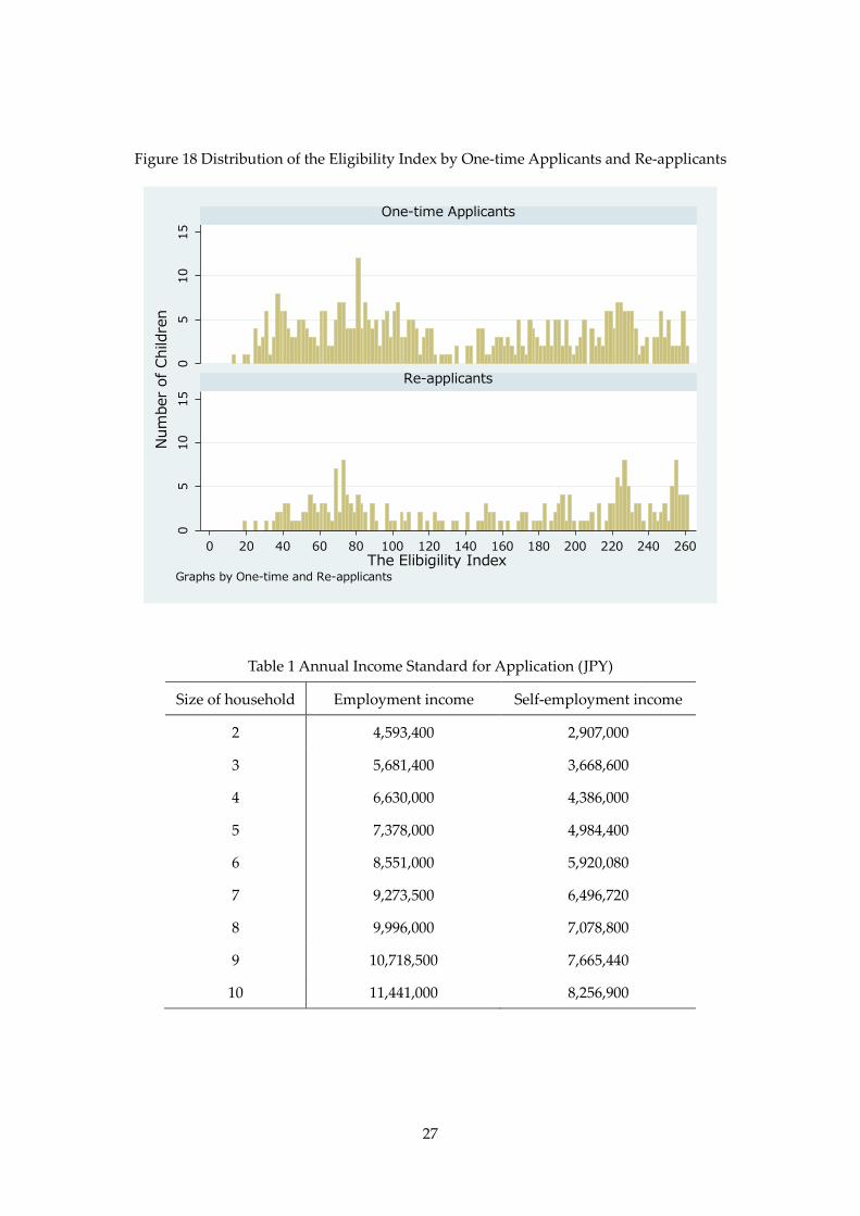
Applicants who hope to receive vouchers must meet the income requirement and the

requirements for disaster victims of the Great East Japan Earthquake. Regarding the income

requirement, the applicants must satisfy at least one of following two conditions: (i) receive

public assistance or (ii) household annual income is less than or equal to the income

standard as Table 1 shows. Regarding the requirement for a disaster victim of the

earthquake, the applicants must satisfy at least one of following three conditions: (i) own

residence was fully or partly destroyed by the earthquake; (ii) had at least one family

member die or is still missing because of the earthquake; (iii) at least one family member or

the applicant was injured or impaired because of the earthquake, or (iv) at least one family

member became unemployed because of the earthquake.

The eligibility index was used to select applicants, which has a maximum value of 300

and consists of the severity of the applicant’s household economic conditions (200), how

soon the applicant has to take the entrance examination (to high school or university) (60),

and the applicant’s motivation for learning as measured by a questionnaire (40). The higher

the eligibility index value, the more likely that the applicant will receive the voucher. The

CFC selected 263 beneficiaries, out of which 127 continued to receive benefits from FY 2013.

Out of the 263, 136 were selected as having the highest eligibility index value from 1,807

total applications during FY 2014. Because elementary school student applicants did not

answer the questionnaire, their motivation for learning was uniformly scored at 20. All the

applicants from households receiving public assistance were selected as beneficiaries

regardless of their eligibility index score.

3 Empirical Strategy and Data

3.1 Methodology As mentioned previously, because the eligibility index is used to select voucher

beneficiaries, we exploit an RDD to estimate the causal effect of shadow education vouchers

7

on several educational outcomes. Because the eligibility index was not used to select 127

out of the 263 beneficiaries who continued to receive beneficiaries from FY 2013, we exclude

these beneficiaries from our analysis. In addition, applicants receiving public assistance are

excluded from the analysis because they were selected as beneficiaries regardless of their

eligibility index score. Elementary school student applicants were also excluded because

they did not answer the questionnaire that the CFC used to survey the outcome variables,

as noted previously. In addition, third graders in high school were excluded from our

analysis because we cannot capture the outcome variables of third-grade non-beneficiaries

in high schools. As subsequently described, ex-post outcome variables of non-beneficiaries

are collected through a survey of reapplicants during the following year. However, because

applicants must be current students, last year’s third-grade high school students are not

included.

Consequently, the number of treated children is 70. To estimate the treatment effect of

the voucher program, we must obtain the ex-post outcome variables, such as academic

achievements and study hours. Although we can obtain the ex-post outcome variables for

beneficiaries through the survey conducted by the CFC at the end of the fiscal year (March

2015), we cannot for non-beneficiaries. However, because approximately one-third of failed

applicants reapplied for the voucher program during the following year, we can use the FY

2015 application to obtain their ex-post outcome variables through a questionnaire.

Therefore, we use the reapplicants as the control group for our analysis.

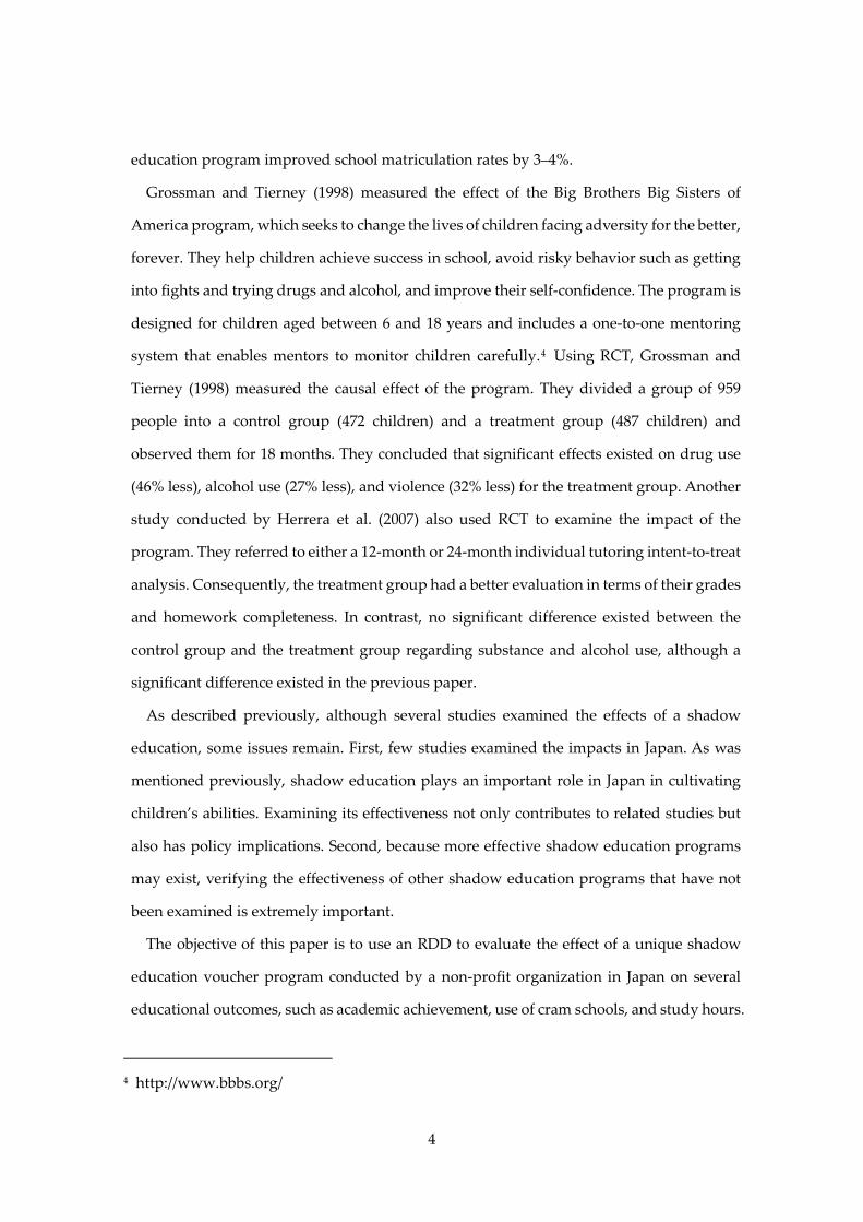
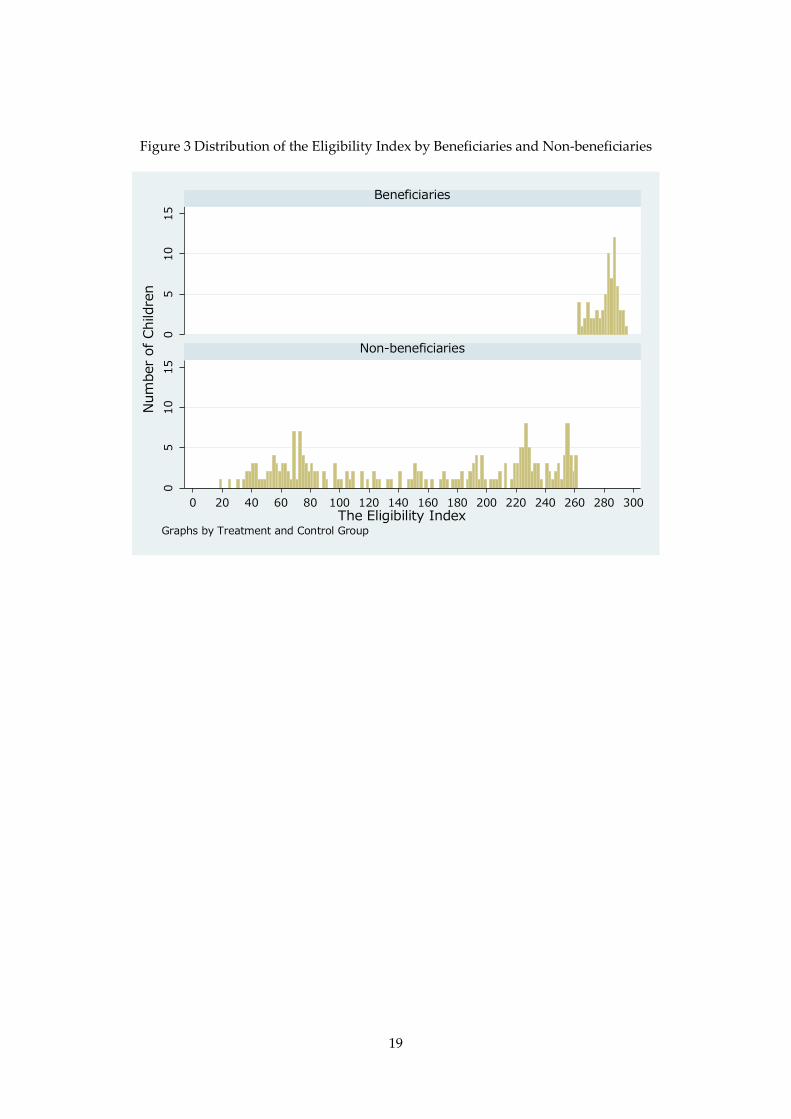
Figure 3 shows the distribution of the eligibility index by beneficiaries and non-

beneficiaries. The eligibility index is called a running variable in the context of an RDD. The

threshold to accept or reject was 262. The applicants whose eligibility index score was

greater than or equal to 262 were beneficiaries, and the applicants with a score less than 262

were non-beneficiaries, making 262 the cutoff in the context of an RDD. This variation is

exogenous and cannot be manipulated by the applicants around the cutoff. Fortunately, no

other clear institutional thresholds exist that could generate confounding discontinuities at

262.

Because our sample is somewhat small, we exploit the local randomization approach

8

proposed by Cattaneo et al. (2017a, 2017b).6 In this framework, we postulate that treatment

assignments are randomized near the cutoff. In other words, the observations closest to the

cutoff are viewed as being part of a local randomized experiment. For a small sample,

although estimation and inference on the basis of large-sample approximations might be

invalid, a local randomization approach that employs a randomization inference is robust.

The estimation steps proposed by Cattaneo et al. (2017a, 2017b) are as follows.7

1. Set an initial small window near the cutoff.

2. For each of the ex-ante covariates, conduct a test of the null hypothesis of no effect

of treatment on the covariates. We employ the Fisherian inference approach, which

is valid in any finite sample and use the so-called sharp null hypothesis to conduct

statistical tests. The minimum p-values are taken from the k tests.

3. If the minimum p-value obtained in step 2 is larger than some prespecified level (0.15

in this paper), a larger window is chosen, and step 2 is revisited to calculate the

minimum p-value. The process is repeated until the minimum p-value is less than

0.15. The selected window is the largest window such that the minimum p-value is

equal to or is larger than 0.15.

4. Because a local randomization approach is only plausible in a very small window

around the cutoff, we employ the Fisherian inference approach to estimate the

treatment effects.

3.2 Data, Descriptive Statistics, and Preliminary Analyses 3.2.1 Data

We utilize surveys conducted by the CFC to estimate the effects of a shadow education

on various outcomes. As mentioned previously, the CFC carried out a survey for applicants

6 As Cattaneo et al. (2017a, 2017b) pointed out, a global polynomial approach is widely

recognized as not delivering desirable point estimates near the boundary. 7 We utilize the Stata package “rdlocrand” produced by Calonico et al. (2016) to estimate

the treatment effects.

9

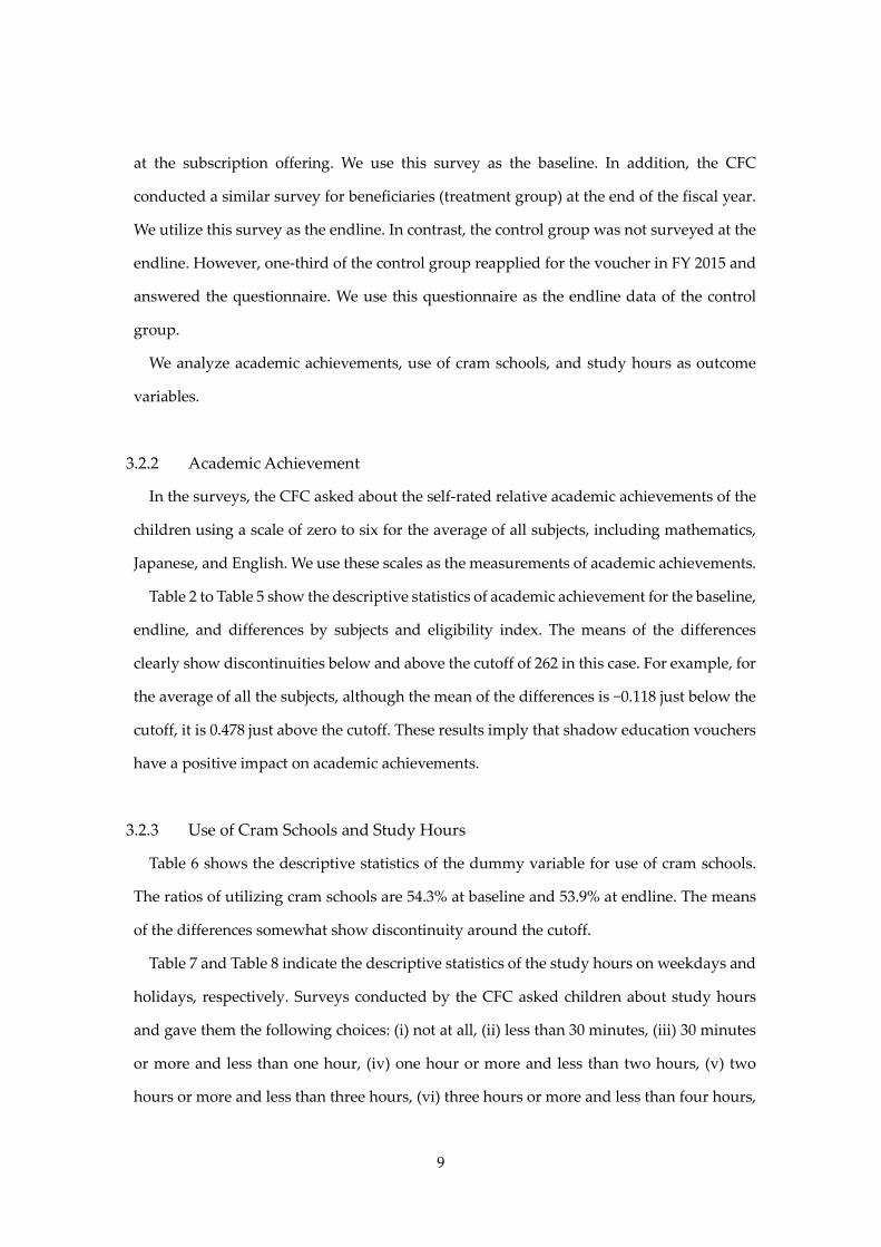
at the subscription offering. We use this survey as the baseline. In addition, the CFC

conducted a similar survey for beneficiaries (treatment group) at the end of the fiscal year.

We utilize this survey as the endline. In contrast, the control group was not surveyed at the

endline. However, one-third of the control group reapplied for the voucher in FY 2015 and

answered the questionnaire. We use this questionnaire as the endline data of the control

group.

We analyze academic achievements, use of cram schools, and study hours as outcome

variables.

3.2.2 Academic Achievement

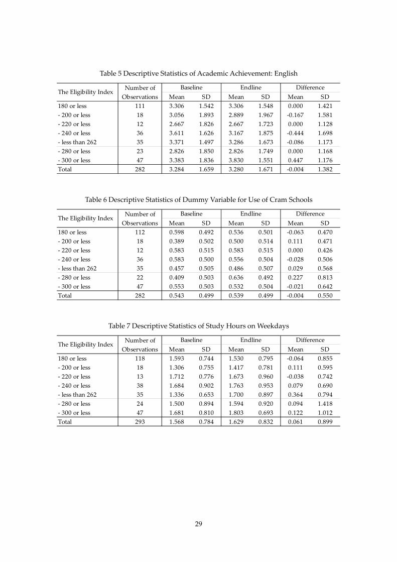
In the surveys, the CFC asked about the self-rated relative academic achievements of the

children using a scale of zero to six for the average of all subjects, including mathematics,

Japanese, and English. We use these scales as the measurements of academic achievements.

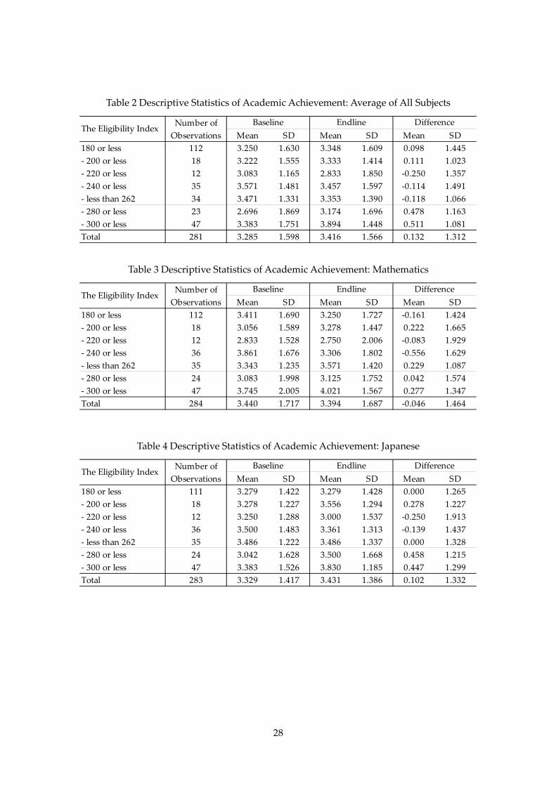
Table 2 to Table 5 show the descriptive statistics of academic achievement for the baseline,

endline, and differences by subjects and eligibility index. The means of the differences

clearly show discontinuities below and above the cutoff of 262 in this case. For example, for

the average of all the subjects, although the mean of the differences is −0.118 just below the

cutoff, it is 0.478 just above the cutoff. These results imply that shadow education vouchers

have a positive impact on academic achievements.

3.2.3 Use of Cram Schools and Study Hours

Table 6 shows the descriptive statistics of the dummy variable for use of cram schools.

The ratios of utilizing cram schools are 54.3% at baseline and 53.9% at endline. The means

of the differences somewhat show discontinuity around the cutoff.

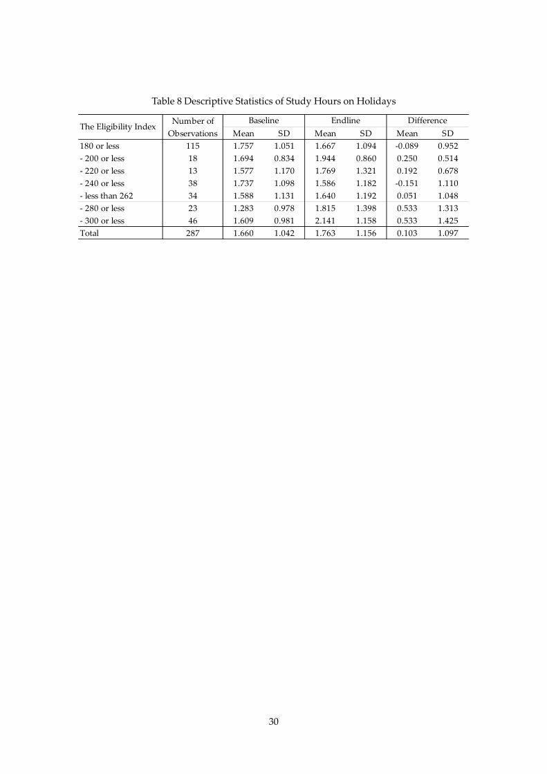
Table 7 and Table 8 indicate the descriptive statistics of the study hours on weekdays and

holidays, respectively. Surveys conducted by the CFC asked children about study hours

and gave them the following choices: (i) not at all, (ii) less than 30 minutes, (iii) 30 minutes

or more and less than one hour, (iv) one hour or more and less than two hours, (v) two

hours or more and less than three hours, (vi) three hours or more and less than four hours,

10

or (vii) four hours or more. We use the medians of each choice to convert these choices into

hours. For example, we convert choice (ii) into 0.25 hours (15 minutes).

The means of study hours on weekdays are 1.568 at baseline and 1.629 at endline,

respectively. The means of the differences do not indicate discontinuity around the cutoff.

However, the means of the differences in study hours on holidays obviously indicate

discontinuity around the cutoff. Although the mean of the difference is 0.051 just below the

cutoff, it is 0.533 just above the cutoff. This fact might indicate that recipients of shadow

education vouchers increased their study hours on holidays by approximately 30 minutes

relative to non-recipients’ study hours.

4 Estimation Results 4.1 Window Selection

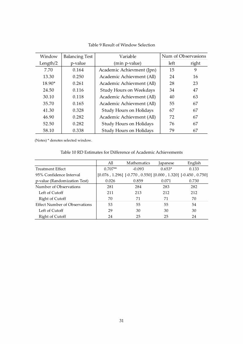
Before estimating the treatment effects, we must use the window-selection algorithm

explained in section 3 to select the desired window. We utilize all the outcome variables at

baseline to select the window. Table 9 shows the result of the window selection. The first

column provides the window length of each window divided by two. The second column

provides the minimum p-value of the balancing test. The third column contains the name

of the corresponding variable associated with the p-value in the second column. The fourth

and fifth columns show the number of observations to the left and right of the cutoff inside

each window.

The largest window for which the second column is equal to or greater than 0.15 is 18.90.

Therefore, our window becomes [243.1(=262 − 18.9), 280.9(=262 + 18.9)] and contains 51

observations.

4.2 Academic Achievement In this section, we show the plots and the estimation results by exploiting an RDD.

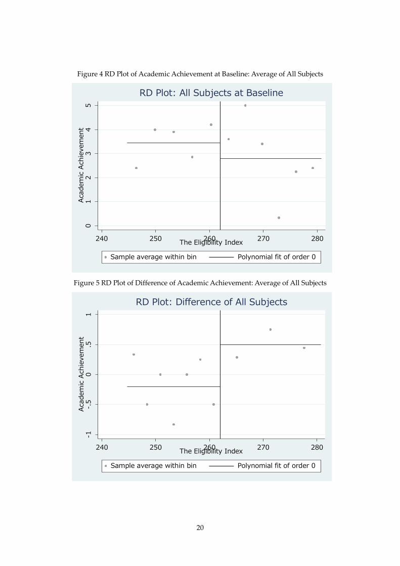
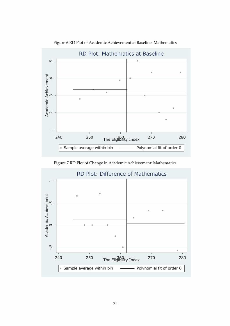
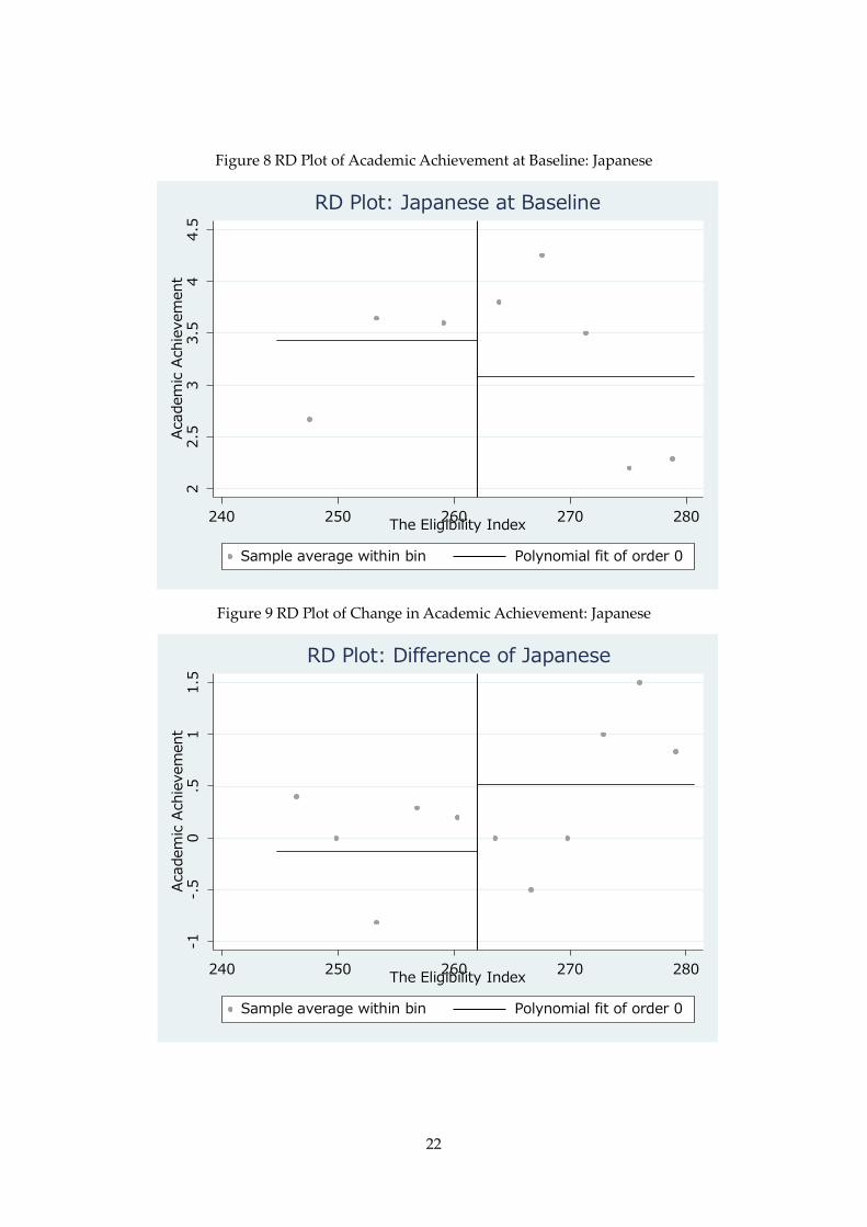
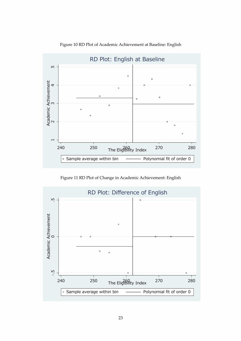
Figure 4 to Figure 11 indicate the RD plots for academic achievement at baseline (pre-

intervention) and changes in those from baseline to endline by subject. The differences

between beneficiaries and non-beneficiaries are not observed at baseline. These facts

11

indicate that the treatment and control groups are quite similar before implementing the

voucher program, making these two groups comparable when estimating the causal effects

of the program. However, the changes in academic achievement for the average of all the

subjects and Japanese from baseline to endline seem quite large. These changes imply that

shadow education vouchers might have positive effects on some academic achievements.

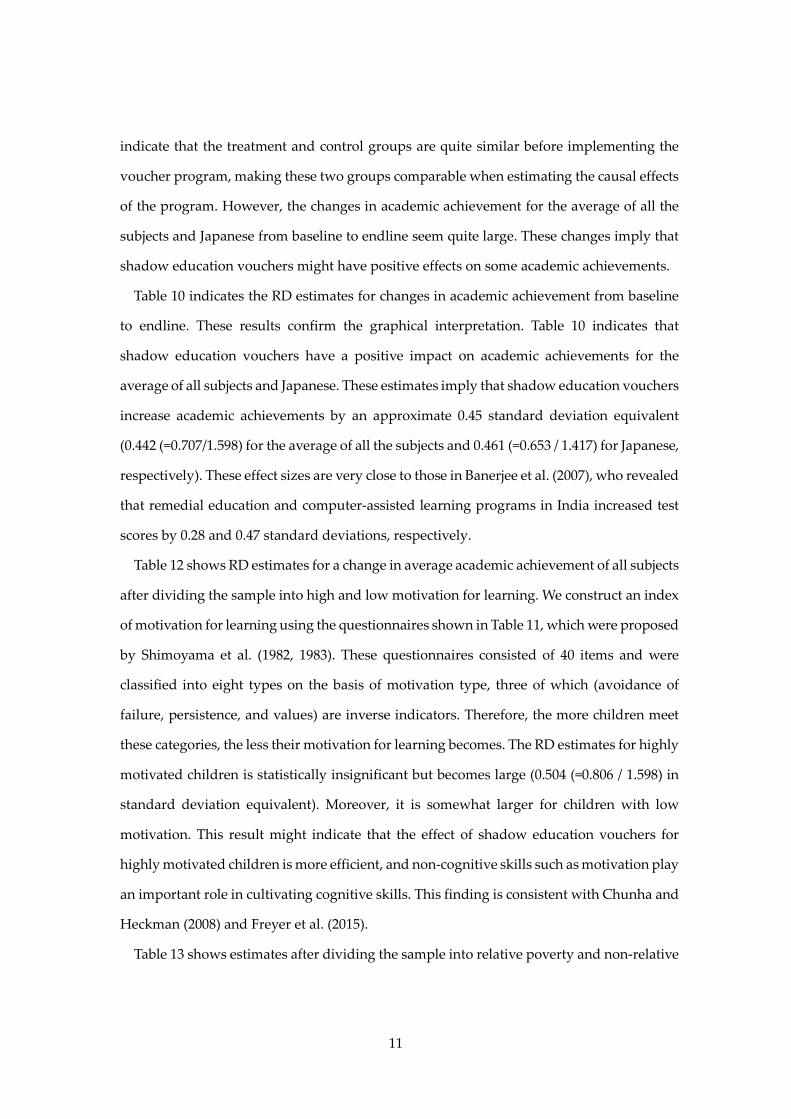
Table 10 indicates the RD estimates for changes in academic achievement from baseline

to endline. These results confirm the graphical interpretation. Table 10 indicates that

shadow education vouchers have a positive impact on academic achievements for the

average of all subjects and Japanese. These estimates imply that shadow education vouchers

increase academic achievements by an approximate 0.45 standard deviation equivalent

(0.442 (=0.707/1.598) for the average of all the subjects and 0.461 (=0.653 / 1.417) for Japanese,

respectively). These effect sizes are very close to those in Banerjee et al. (2007), who revealed

that remedial education and computer-assisted learning programs in India increased test

scores by 0.28 and 0.47 standard deviations, respectively.

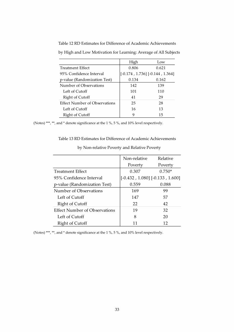
Table 12 shows RD estimates for a change in average academic achievement of all subjects

after dividing the sample into high and low motivation for learning. We construct an index

of motivation for learning using the questionnaires shown in Table 11, which were proposed

by Shimoyama et al. (1982, 1983). These questionnaires consisted of 40 items and were

classified into eight types on the basis of motivation type, three of which (avoidance of

failure, persistence, and values) are inverse indicators. Therefore, the more children meet

these categories, the less their motivation for learning becomes. The RD estimates for highly

motivated children is statistically insignificant but becomes large (0.504 (=0.806 / 1.598) in

standard deviation equivalent). Moreover, it is somewhat larger for children with low

motivation. This result might indicate that the effect of shadow education vouchers for

highly motivated children is more efficient, and non-cognitive skills such as motivation play

an important role in cultivating cognitive skills. This finding is consistent with Chunha and

Heckman (2008) and Freyer et al. (2015).

Table 13 shows estimates after dividing the sample into relative poverty and non-relative

12

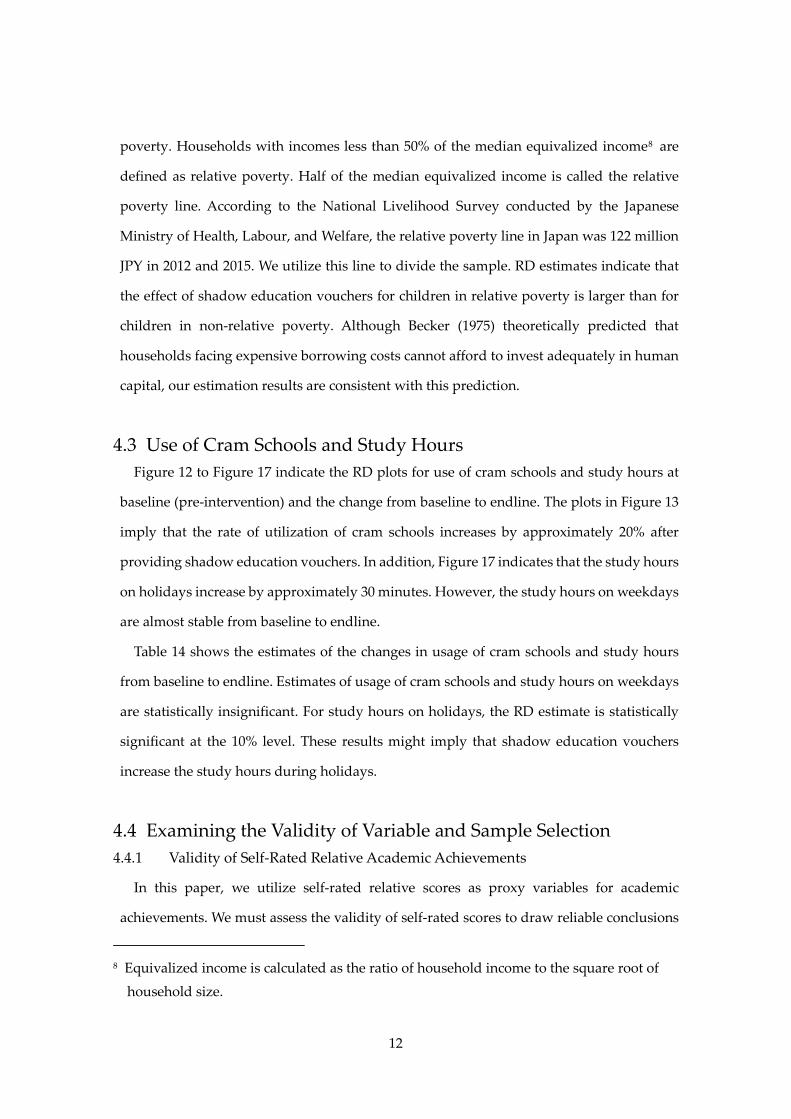
poverty. Households with incomes less than 50% of the median equivalized income8 are

defined as relative poverty. Half of the median equivalized income is called the relative

poverty line. According to the National Livelihood Survey conducted by the Japanese

Ministry of Health, Labour, and Welfare, the relative poverty line in Japan was 122 million

JPY in 2012 and 2015. We utilize this line to divide the sample. RD estimates indicate that

the effect of shadow education vouchers for children in relative poverty is larger than for

children in non-relative poverty. Although Becker (1975) theoretically predicted that

households facing expensive borrowing costs cannot afford to invest adequately in human

capital, our estimation results are consistent with this prediction.

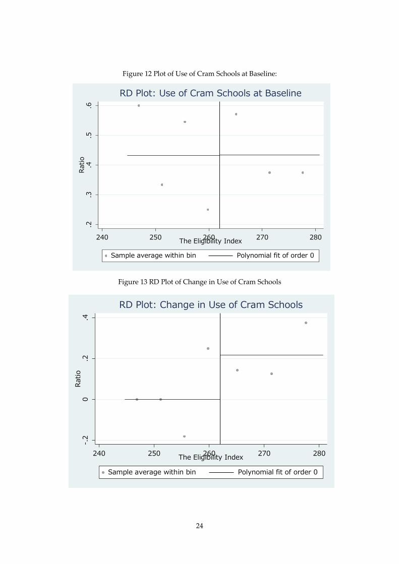
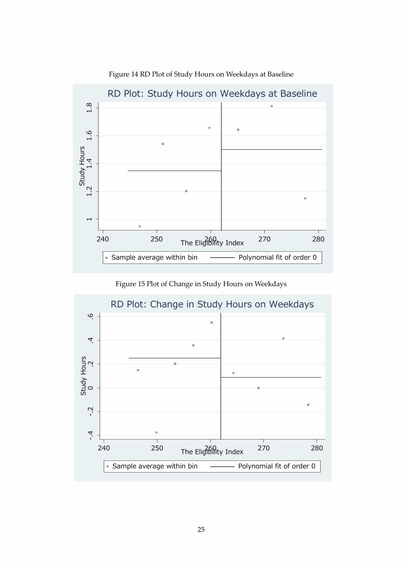
4.3 Use of Cram Schools and Study Hours Figure 12 to Figure 17 indicate the RD plots for use of cram schools and study hours at

baseline (pre-intervention) and the change from baseline to endline. The plots in Figure 13

imply that the rate of utilization of cram schools increases by approximately 20% after

providing shadow education vouchers. In addition, Figure 17 indicates that the study hours

on holidays increase by approximately 30 minutes. However, the study hours on weekdays

are almost stable from baseline to endline.

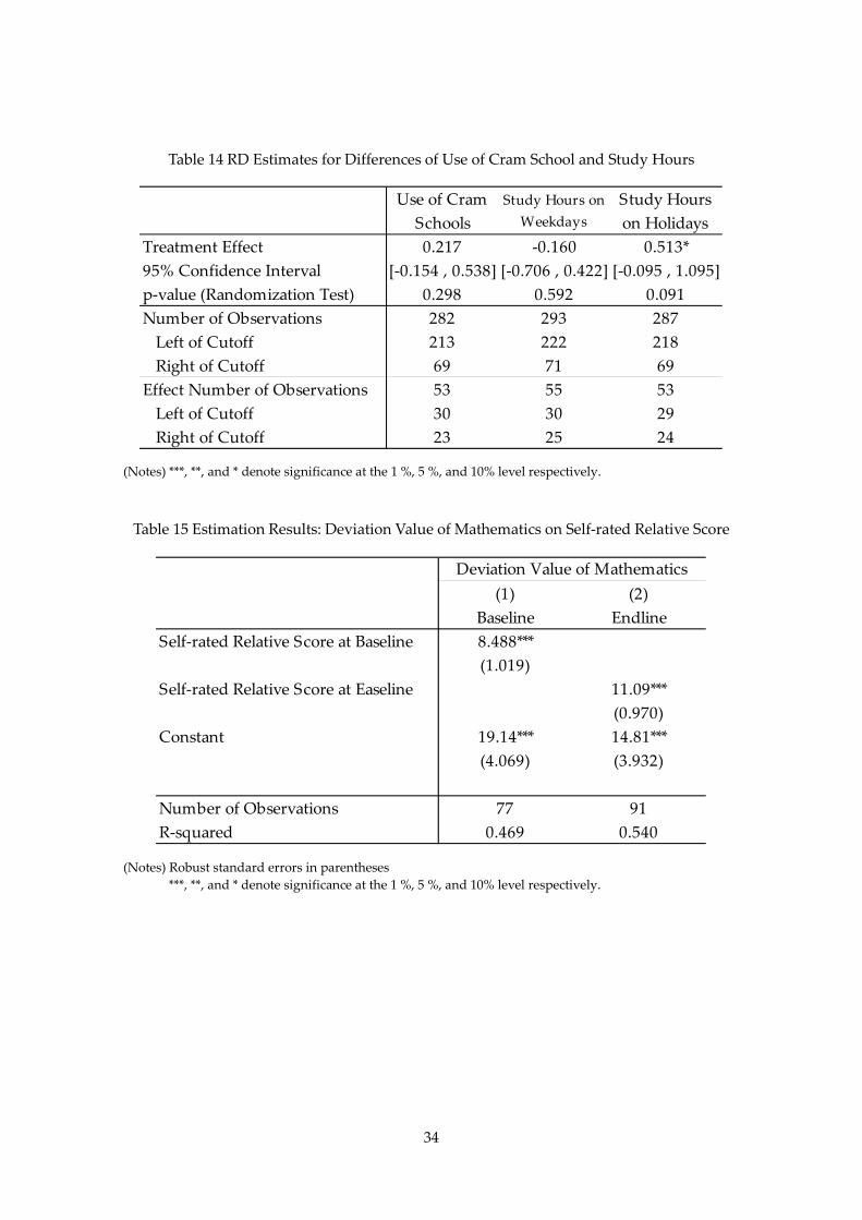
Table 14 shows the estimates of the changes in usage of cram schools and study hours

from baseline to endline. Estimates of usage of cram schools and study hours on weekdays

are statistically insignificant. For study hours on holidays, the RD estimate is statistically

significant at the 10% level. These results might imply that shadow education vouchers

increase the study hours during holidays.

4.4 Examining the Validity of Variable and Sample Selection 4.4.1 Validity of Self-Rated Relative Academic Achievements

In this paper, we utilize self-rated relative scores as proxy variables for academic

achievements. We must assess the validity of self-rated scores to draw reliable conclusions

8 Equivalized income is calculated as the ratio of household income to the square root of

household size.

13

from our estimation results. The CFC conducted tests on recipients who were junior high

school students to measure academic achievements in mathematics by using commercially

available tests at baseline and endline. We examine the validity of the self-rated score to

utilize those tests.

Table 15 presents the estimation results of regressing the deviation value of mathematics

on the self-rated relative score. The first column of Table 15 is the result at baseline, and the

second column is the result at endline. Both estimates are significantly positive and the R-

squared coefficients are 0.469 at baseline and 0.540 at endline, respectively. Therefore, self-

rated relative scores are viewed as appropriate measures of academic achievements.

4.4.2 Sample Selection of Control Group

As explained previously, we utilize the reapplicants who failed the 2014 application as

our control group. If the reapplicants have systematically different characteristics than one-

time applicants, these differences might bias our estimation results.

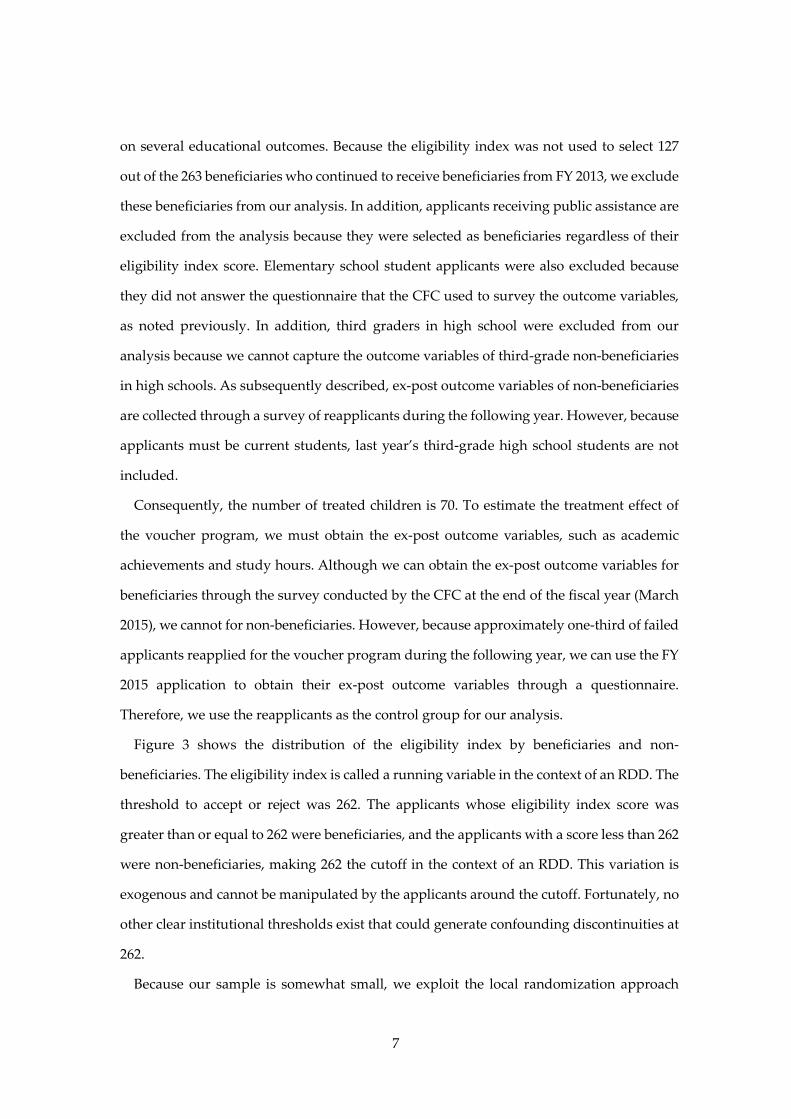
Figure 18 shows the distribution of the eligibility index by the one-time applicants and

the reapplicants and indicates that systematical differences between two groups do not

seem to be observed. Table 16 indicates the estimation results from using a probit model to

regress a dummy variable of reapplicants on our outcome variables at baseline. The

coefficients shown in Table 16 indicate marginal effects. The result implies that the eligibility

index is positively related to reapplications. However, the magnitude is not large and, even

if the eligibility index increases by 100 points, the probability of reapplication is increased

by approximately 7.6% only.

Therefore, the utilization of the reapplicants as our control group does not seem to distort

our estimation results.

4.4.3 Sample Selection of Treatment Group

As section 2 explains, our running variable is calculated by summing up three factors.

Because of how soon they will take the entrance examination accounts for 60 of the running

variable, which has a maximum value of 300 and our cutoff is 262, most of the beneficiaries

14

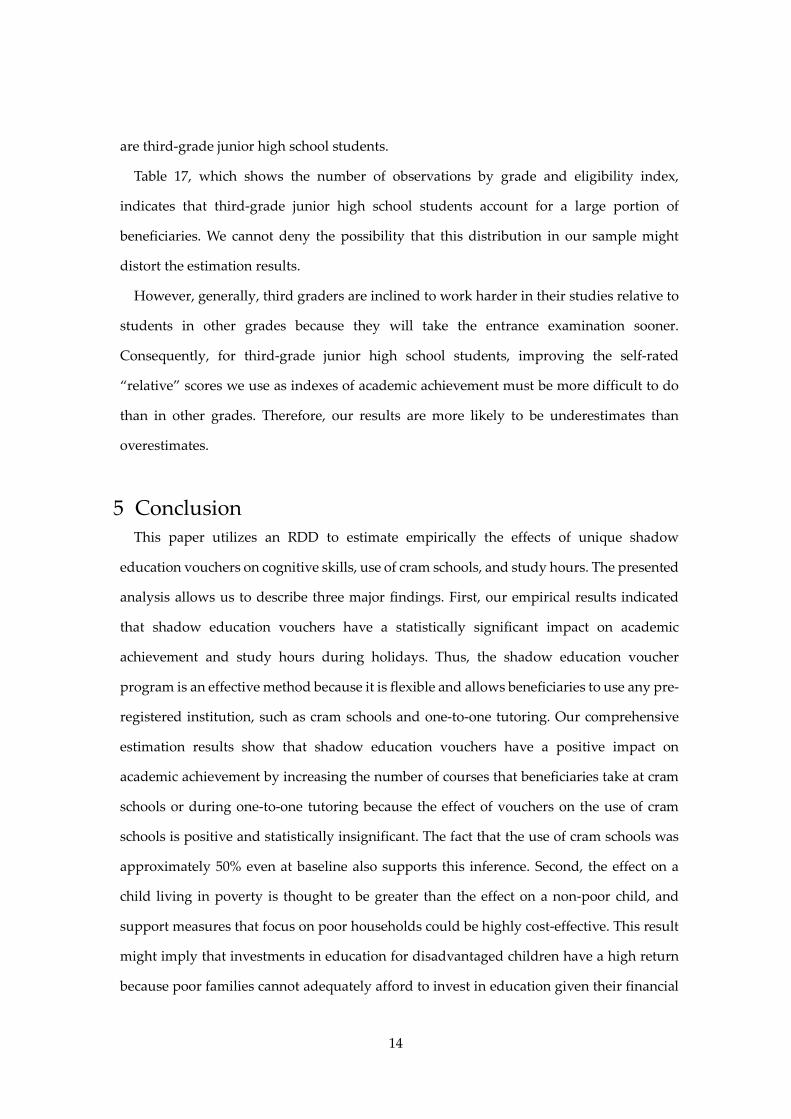
are third-grade junior high school students.

Table 17, which shows the number of observations by grade and eligibility index,

indicates that third-grade junior high school students account for a large portion of

beneficiaries. We cannot deny the possibility that this distribution in our sample might

distort the estimation results.

However, generally, third graders are inclined to work harder in their studies relative to

students in other grades because they will take the entrance examination sooner.

Consequently, for third-grade junior high school students, improving the self-rated

“relative” scores we use as indexes of academic achievement must be more difficult to do

than in other grades. Therefore, our results are more likely to be underestimates than

overestimates.

5 Conclusion This paper utilizes an RDD to estimate empirically the effects of unique shadow

education vouchers on cognitive skills, use of cram schools, and study hours. The presented

analysis allows us to describe three major findings. First, our empirical results indicated

that shadow education vouchers have a statistically significant impact on academic

achievement and study hours during holidays. Thus, the shadow education voucher

program is an effective method because it is flexible and allows beneficiaries to use any pre-

registered institution, such as cram schools and one-to-one tutoring. Our comprehensive

estimation results show that shadow education vouchers have a positive impact on

academic achievement by increasing the number of courses that beneficiaries take at cram

schools or during one-to-one tutoring because the effect of vouchers on the use of cram

schools is positive and statistically insignificant. The fact that the use of cram schools was

approximately 50% even at baseline also supports this inference. Second, the effect on a

child living in poverty is thought to be greater than the effect on a non-poor child, and

support measures that focus on poor households could be highly cost-effective. This result

might imply that investments in education for disadvantaged children have a high return

because poor families cannot adequately afford to invest in education given their financial

15

constraints. Finally, the impacts of shadow education vouchers for highly motivated

children might be somewhat greater than for children with low motivation. This result

implies that enhancing motivation before providing learning support is crucial to efficiently

improving students’ cognitive ability. This implication might be consistent with Freyer et

al. (2015), who revealed that children with above-median non-cognitive scores before

treatment accrued the greatest benefits from treatment. In addition, Chuha and Heckman

(2008) revealed that non-cognitive skills promote the formation of cognitive skills but that

cognitive skills do not promote the formation of non-cognitive skills. Chuha and Heckman

(2008) might also have findings that are consistent with our results.

Our analyses have several limitations. The first limitation concerns the external validity.

Our empirical results are for the unusual situation after the Great East Japan Earthquake,

and the program we examined is for disadvantaged children. Especially in Japan,

estimating the causal effects of policies and practices is rare; yet, further studies are required

to examine whether the results in this paper can be generalized. Second, we need to reveal

the underlying structure of the program provided by the CFC, which consists of not only

shadow education vouchers but also mentoring support from volunteers of university

students. Because we estimate only the effect of the entire program, each effect from

financial support and mentoring support are yet to be revealed. In addition, future studies

need to explore the efficiency of the program. Third, in this paper, we utilize self-rated

scores as indicators of academic achievement. We cannot deny that the scores have some

biases or noise, and our results need to be reexamined by utilizing more objective indicators.

Finally, as previously mentioned, our control group consists of only reapplicants during the

following year. In addition, the treatment group mainly consists of third-grade junior high

school students. We cannot deny the possibility that these issues with our sample might

distort the estimation results.

16

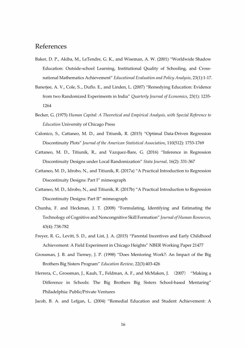
References

Baker, D. P., Akiba, M., LeTendre, G. K., and Wiseman, A. W. (2001) “Worldwide Shadow

Education: Outside-school Learning, Institutional Quality of Schooling, and Cross-

national Mathematics Achievement” Educational Evaluation and Policy Analysis, 23(1):1-17.

Banerjee, A. V., Cole, S.., Duflo. E., and Linden, L. (2007) “Remedying Education: Evidence

from two Randomized Experiments in India” Quarterly Journal of Economics, 23(1): 1235-

1264

Becker, G. (1975) Human Capital: A Theoretical and Empirical Analysis, with Special Reference to

Education University of Chicago Press

Calonico, S., Cattaneo, M. D., and Titiunik, R. (2015) “Optimal Data-Driven Regression

Discontinuity Plots” Journal of the American Statistical Association, 110(512): 1753-1769

Cattaneo, M. D., Titiunik, R., and Vazquez-Bare, G. (2016) “Inference in Regression

Discontinuity Designs under Local Randomization” Stata Journal, 16(2): 331-367

Cattaneo, M. D., Idrobo, N., and Titiunik, R. (2017a) “A Practical Introduction to Regression

Discontinuity Designs: Part I” mimeograph

Cattaneo, M. D., Idrobo, N., and Titiunik, R. (2017b) “A Practical Introduction to Regression

Discontinuity Designs: Part II” mimeograph

Chunha, F. and Heckman, J. T. (2008) “Formulating, Identifying and Estimating the

Technology of Cognitive and Noncongnitive Skill Formation” Journal of Human Resources,

43(4): 738-782

Freyer, R. G., Levitt, S. D., and List, J. A. (2015) “Parental Incentives and Early Childhood

Achievement: A Field Experiment in Chicago Heights” NBER Working Paper 21477

Grossman, J. B. and Tierney, J. P. (1998) “Does Mentoring Work?: An Impact of the Big

Brothers Big Sisters Program” Education Review, 22(3):403-426

Herrera, C., Grossman, J., Kauh, T., Feldman, A. F., and McMaken, J. （2007） “Making a

Difference in Schools: The Big Brothers Big Sisters School-based Mentaring”

Philadelphia: Public/Private Ventures

Jacob, B. A. and Lefgan, L. (2004) “Remedial Education and Student Achievement: A

17

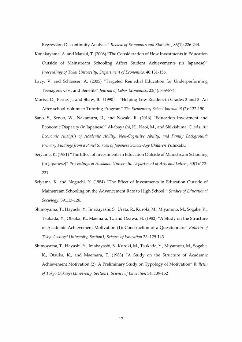
Regression-Discontinuity Analysis” Review of Economics and Statistics, 86(1): 226-244.

Konakayama, A. and Matsui, T. (2008) “The Consideration of How Investments in Education

Outside of Mainstream Schooling Affect Student Achievements (in Japanese)”

Proceedings of Tokai University, Department of Economics, 40:131-158.

Lavy, V. and Schlosser, A. (2005) “Targeted Remedial Education for Underperforming

Teenagers: Cost and Benefits” Journal of Labor Economics, 23(4): 839-874

Moriss, D., Perne, J., and Shaw, B.（1990） “Helping Low Readers in Grades 2 and 3: An

After-school Volunteer Tutoring Program“ The Elementary School Journal 91(2): 132-150

Sano, S., Senoo, W., Nakamura, R., and Nozaki, R. (2016) “Education Investment and

Economic Disparity (in Japanese)” Akabayashi, H., Naoi, M., and Shikishima, C. eds. An

Economic Analysis of Academic Ability, Non-Cognitive Ability, and Family Background:

Primary Findings from a Panel Survey of Japanese School-Age Children Yuhikaku

Seiyama, K. (1981) “The Effect of Investments in Education Outside of Mainstream Schooling

(in Japanese)” Proceedings of Hokkaido University, Department of Arts and Letters, 30(1):173-

221.

Seiyama, K. and Noguchi, Y. (1984) “The Effect of Investments in Education Outside of

Mainstream Schooling on the Advancement Rate to High School.” Studies of Educational

Sociology, 39:113-126.

Shimoyama, T., Hayashi, Y., Imabayashi, S., Urata, R., Kuroki, M., Miyamoto, M., Sogabe, K.,

Tsukada, Y., Otsuka, K., Maemara, T., and Ozawa, H. (1982) “A Study on the Structure

of Academic Achievement Motivation (1): Construction of a Questionnare” Bulletin of

Tokyo Gakugei University, Section1, Science of Education 33: 129-143

Shimoyama, T., Hayashi, Y., Imabayashi, S., Kuroki, M., Tsukada, Y., Miyamoto, M., Sogabe,

K., Otsuka, K., and Maemara, T. (1983) “A Study on the Structure of Academic

Achievement Motivation (2): A Preliminary Study on Typology of Motivation” Bulletin

of Tokyo Gakugei University, Section1, Science of Education 34: 139-152

18

Figure 1 Changes in average expenditure on one-to-one tutoring and cramming school

(Source) Ministry of Education, Culture, Sports, Science and Technology

Figure 2 Average expenditure on supplementary education

by household annual income in 2016

(Source) Ministry of Education, Culture, Sports, Science and Technology

0

50

100

150

200

250

1994 1996 1998 2000 2002 2004 2006 2008 2010 2012 2014 2016

Public Junior High School Private Junior Hight School

Public High School Private High School

(Fiscal Year)

Aver

age

Expe

nditu

re (t

hous

and

JPY

)

0

100

200

300

400

less than 4 4-6 6-8 8-10 10-12 12 or more

Public Junior High School Private Junior Hight School

Public High School Private High School

Household annual income (million JPY)

Aver

age

Expe

nditu

re (t

hous

and

JPY

)

19

Figure 3 Distribution of the Eligibility Index by Beneficiaries and Non-beneficiaries

05

1015

05

1015

0 20 40 60 80 100 120 140 160 180 200 220 240 260 280 300

Beneficiaries

Non-beneficiaries

Num

ber

of C

hild

ren

The Eligibility IndexGraphs by Treatment and Control Group

20

Figure 4 RD Plot of Academic Achievement at Baseline: Average of All Subjects

Figure 5 RD Plot of Difference of Academic Achievement: Average of All Subjects

01

23

45

Acad

emic

Ach

ieve

men

t

240 250 260 270 280The Eligibility Index

Sample average within bin Polynomial fit of order 0

RD Plot: All Subjects at Baseline-1

-.5

0.5

1Ac

adem

ic A

chie

vem

ent



RD Plot: Difference of All Subjects

21

Figure 6 RD Plot of Academic Achievement at Baseline: Mathematics

Figure 7 RD Plot of Change in Academic Achievement: Mathematics

12

34

5Ac

adem

ic A

chie

vem

ent



RD Plot: Mathematics at Baseline-.

50

.51

Acad

emic

Ach

ieve

men

t



RD Plot: Difference of Mathematics

22

Figure 8 RD Plot of Academic Achievement at Baseline: Japanese

Figure 9 RD Plot of Change in Academic Achievement: Japanese

22.

53

3.5

44.

5Ac

adem

ic A

chie

vem

ent



RD Plot: Japanese at Baseline-1

-.5

0.5

11.

5Ac

adem

ic A

chie

vem

ent



RD Plot: Difference of Japanese

23

Figure 10 RD Plot of Academic Achievement at Baseline: English

Figure 11 RD Plot of Change in Academic Achievement: English

12

34

5Ac

adem

ic A

chie

vem

ent



RD Plot: English at Baseline-.

50

.5Ac

adem

ic A

chie

vem

ent



RD Plot: Difference of English

24

Figure 12 Plot of Use of Cram Schools at Baseline:

Figure 13 RD Plot of Change in Use of Cram Schools

.2.3

.4.5

.6Ra

tio



RD Plot: Use of Cram Schools at Baseline-.

20

.2.4

Ratio



RD Plot: Change in Use of Cram Schools

25

Figure 14 RD Plot of Study Hours on Weekdays at Baseline

Figure 15 Plot of Change in Study Hours on Weekdays

11.

21.

41.

61.

8St

udy

Hou

rs



RD Plot: Study Hours on Weekdays at Baseline-.

4-.

20

.2.4

.6St

udy

Hou

rs



RD Plot: Change in Study Hours on Weekdays

26

Figure 16 RD Plot of Study Hours on Holidays at Baseline

Figure 17 RD Plot of Change in Study Hours on Holidays

.51

1.5

22.

5St

udy

Hou

rs



RD Plot: Study Hours on Holidays-1

-.5

0.5

1St

udy

Hou

rs



RD Plot: Change in Study Hours on Holidays

27

Figure 18 Distribution of the Eligibility Index by One-time Applicants and Re-applicants

Table 1 Annual Income Standard for Application (JPY)

Size of household Employment income Self-employment income

2 4,593,400 2,907,000

3 5,681,400 3,668,600

4 6,630,000 4,386,000

5 7,378,000 4,984,400

6 8,551,000 5,920,080

7 9,273,500 6,496,720

8 9,996,000 7,078,800

9 10,718,500 7,665,440

10 11,441,000 8,256,900

05

1015

05

1015

0 20 40 60 80 100 120 140 160 180 200 220 240 260

One-time Applicants

Re-applicants

Num

ber

of C

hild

ren

The Elibigility IndexGraphs by One-time and Re-applicants

28

Table 2 Descriptive Statistics of Academic Achievement: Average of All Subjects

Table 3 Descriptive Statistics of Academic Achievement: Mathematics

Table 4 Descriptive Statistics of Academic Achievement: Japanese

Mean SD Mean SD Mean SD180 or less 112 3.250 1.630 3.348 1.609 0.098 1.445- 200 or less 18 3.222 1.555 3.333 1.414 0.111 1.023- 220 or less 12 3.083 1.165 2.833 1.850 -0.250 1.357- 240 or less 35 3.571 1.481 3.457 1.597 -0.114 1.491- less than 262 34 3.471 1.331 3.353 1.390 -0.118 1.066- 280 or less 23 2.696 1.869 3.174 1.696 0.478 1.163- 300 or less 47 3.383 1.751 3.894 1.448 0.511 1.081Total 281 3.285 1.598 3.416 1.566 0.132 1.312

The Eligibility Index Number ofObservations

Baseline Endline Difference

Mean SD Mean SD Mean SD180 or less 112 3.411 1.690 3.250 1.727 -0.161 1.424- 200 or less 18 3.056 1.589 3.278 1.447 0.222 1.665- 220 or less 12 2.833 1.528 2.750 2.006 -0.083 1.929- 240 or less 36 3.861 1.676 3.306 1.802 -0.556 1.629- less than 262 35 3.343 1.235 3.571 1.420 0.229 1.087- 280 or less 24 3.083 1.998 3.125 1.752 0.042 1.574- 300 or less 47 3.745 2.005 4.021 1.567 0.277 1.347Total 284 3.440 1.717 3.394 1.687 -0.046 1.464



Mean SD Mean SD Mean SD180 or less 111 3.279 1.422 3.279 1.428 0.000 1.265- 200 or less 18 3.278 1.227 3.556 1.294 0.278 1.227- 220 or less 12 3.250 1.288 3.000 1.537 -0.250 1.913- 240 or less 36 3.500 1.483 3.361 1.313 -0.139 1.437- less than 262 35 3.486 1.222 3.486 1.337 0.000 1.328- 280 or less 24 3.042 1.628 3.500 1.668 0.458 1.215- 300 or less 47 3.383 1.526 3.830 1.185 0.447 1.299Total 283 3.329 1.417 3.431 1.386 0.102 1.332



29

Table 5 Descriptive Statistics of Academic Achievement: English

Table 6 Descriptive Statistics of Dummy Variable for Use of Cram Schools

Table 7 Descriptive Statistics of Study Hours on Weekdays

Mean SD Mean SD Mean SD180 or less 111 3.306 1.542 3.306 1.548 0.000 1.421- 200 or less 18 3.056 1.893 2.889 1.967 -0.167 1.581- 220 or less 12 2.667 1.826 2.667 1.723 0.000 1.128- 240 or less 36 3.611 1.626 3.167 1.875 -0.444 1.698- less than 262 35 3.371 1.497 3.286 1.673 -0.086 1.173- 280 or less 23 2.826 1.850 2.826 1.749 0.000 1.168- 300 or less 47 3.383 1.836 3.830 1.551 0.447 1.176Total 282 3.284 1.659 3.280 1.671 -0.004 1.382



Mean SD Mean SD Mean SD180 or less 112 0.598 0.492 0.536 0.501 -0.063 0.470- 200 or less 18 0.389 0.502 0.500 0.514 0.111 0.471- 220 or less 12 0.583 0.515 0.583 0.515 0.000 0.426- 240 or less 36 0.583 0.500 0.556 0.504 -0.028 0.506- less than 262 35 0.457 0.505 0.486 0.507 0.029 0.568- 280 or less 22 0.409 0.503 0.636 0.492 0.227 0.813- 300 or less 47 0.553 0.503 0.532 0.504 -0.021 0.642Total 282 0.543 0.499 0.539 0.499 -0.004 0.550



Mean SD Mean SD Mean SD180 or less 118 1.593 0.744 1.530 0.795 -0.064 0.855- 200 or less 18 1.306 0.755 1.417 0.781 0.111 0.595- 220 or less 13 1.712 0.776 1.673 0.960 -0.038 0.742- 240 or less 38 1.684 0.902 1.763 0.953 0.079 0.690- less than 262 35 1.336 0.653 1.700 0.897 0.364 0.794- 280 or less 24 1.500 0.894 1.594 0.920 0.094 1.418- 300 or less 47 1.681 0.810 1.803 0.693 0.122 1.012Total 293 1.568 0.784 1.629 0.832 0.061 0.899



30

Table 8 Descriptive Statistics of Study Hours on Holidays

Mean SD Mean SD Mean SD180 or less 115 1.757 1.051 1.667 1.094 -0.089 0.952- 200 or less 18 1.694 0.834 1.944 0.860 0.250 0.514- 220 or less 13 1.577 1.170 1.769 1.321 0.192 0.678- 240 or less 38 1.737 1.098 1.586 1.182 -0.151 1.110- less than 262 34 1.588 1.131 1.640 1.192 0.051 1.048- 280 or less 23 1.283 0.978 1.815 1.398 0.533 1.313- 300 or less 46 1.609 0.981 2.141 1.158 0.533 1.425Total 287 1.660 1.042 1.763 1.156 0.103 1.097



31

Table 9 Result of Window Selection

(Notes) * denotes selected window.

Table 10 RD Estimates for Difference of Academic Achievements

Variable(min p-value) left right

7.70 0.164 Academic Achievment (Jpn) 15 913.30 0.250 Academic Achievment (All) 24 1618.90* 0.261 Academic Achievment (All) 28 2324.50 0.116 Study Hours on Weekdays 34 4730.10 0.118 Academic Achievment (All) 40 6335.70 0.165 Academic Achievment (All) 55 6741.30 0.328 Study Hours on Holidays 67 6746.90 0.282 Academic Achievment (All) 72 6752.50 0.282 Study Hours on Holidays 76 6758.10 0.338 Study Hours on Holidays 79 67

Num of ObservasionsBalancing Testp-value

WindowLength/2

All Mathematics Japanese EnglishTreatment Effect 0.707** -0.093 0.653* 0.13395% Confidence Interval [0.076 , 1.296] [-0.770 , 0.550] [0.000 , 1.320] [-0.450 , 0.750]p-value (Randomization Test) 0.026 0.859 0.071 0.730Number of Observations 281 284 283 282 Left of Cutoff 211 213 212 212 Right of Cutoff 70 71 71 70Effect Number of Observations 53 55 55 54 Left of Cutoff 29 30 30 30 Right of Cutoff 24 25 25 24

32

Table 11 Questionnaires on Motivation for Learning

No. Question Contents Category

i You would feel happy when you are told to do chores by your teacherii You would be encouraged to write a diary when you are told by your teacher that it would help improve your essayiii You can easily start doing chores if you are asked to help by your teacher(s)iv You would like to read the book which your teacher recommended to you for your Japanese studyv You can easily understand questions on the exams because your teacher is very good at teaching vi You would be responsible for your duty (work)vii You are surely resposible for what you are supposed to do on a group presentationviii You do not ususally raise your hand in class because you are afraid of being laughed at for your mistakes 6 Avoidance of Failures (Inverse Indicator)

i You know how well you have done with your exam right after itii You check your test score when it has been returnediii After the exam, you look up the answers to see if you got them correctiv When you study for the exams, you set a goal for your test scorev The more you think the test is impotant for you, the worse your performance on it will be 6 Avoidance of Failures (Inverse Indicator)vi You either ask your teacher or resolve the questions you could not solve on your maths test until you are satisfied 2 Achievement-orientedvii Once you are stuck in the middle of a test, you tend to fail to get the answers for the questions you could normally solve 6 Avoidance of Failures (Inverse Indicator)viii Even if the qustions seem difficult, you try your best to get the answer(s) 2 Achievement-orientedix When things you are supposed to do look somewhat difficult, you feel it is even more difficult because you think you cannot do well 6 Avoidance of Failures (Inverse Indicator)x If you think you can solve the maths story problems, you will try your best until you get the answer even if the problems look difficultxi You peresistently consdier the difficult questions/problems regarding your Japanese class xii You underestimate your achievement because you are unwilling to realise that you have done less than you expected 6 Avoidance of Failures (Inverse Indicator)xiii You immdeately start studing even if you do not like it 2 Achievement-orientedxiv You carefully think if your way of learning is good 5 Self-appraisal

i You study at home as well as at school because you want to know a lot of things 1 Autonomous Learning Attitudesii You think it is not worth studying things you do not want to studyiii You think it would be much more fun without studyingiv You study without being told by your family member(s) to do sov You study the subject you are not good at without being told to do sovi You think you do not have to study if you can get good scores on your exam(s) 8 Values (Inverse Indicator)vii You set goals and plan well when studying 1 Autonomous Learning Attitudesviii You think it will be better to ask someone who knows than putting too much effort into your studies 8 Values (Inverse Indicator)ix You are usually prepared well for class 1 Autonomous Learning Attitudesx You become skeptical about why you study 8 Values (Inverse Indicator)i You think you get bored easilyii You cannot stop watching your favorite TV programme even when it is about time to studyiii You finish your homework within the day no matter how long it takesiv Whenever there is something you have left, you will finish it laterv You tend to get bored with studyingvi You tend to stop studying when solving difficult questions because you get tiredvii When you study, you stop studying if you find something else that interests you moreviii You always finish your homework even if you are a little sick 3 Responsibility

3 Responsibility

8 Values (Inverse Indicator)

1 Autonomous Learning Attitudes

7 Persistence (Inverse Indicator)

7 Persistence (Inverse Indicator)

What doyou think

about Q(i)－Q(viii)?

4 Pliability

3 Responsibility

5 Self-appraisal

2 Achievement-oriented

Abo

ut S

choo

l

Questions

What doyou think

about Q(i)－Q(xiv)?

What doyou think

about Q(i)－Q(x)?

What doyou think

about Q(i)－Q(viii)?

Abo

ut L

earn

ing

33


by High and Low Motivation for Learning: Average of All Subjects

(Notes) ***, **, and * denote significance at the 1 %, 5 %, and 10% level respectively.


by Non-relative Poverty and Relative Poverty


High LowTreatment Effect 0.806 0.62195% Confidence Interval [-0.174 , 1.736] [-0.144 , 1.364]p-value (Randomization Test) 0.134 0.162Number of Observations 142 139 Left of Cutoff 101 110 Right of Cutoff 41 29Effect Number of Observations 25 28 Left of Cutoff 16 13 Right of Cutoff 9 15

Non-relativePoverty

RelativePoverty

Treatment Effect 0.307 0.750*95% Confidence Interval [-0.432 , 1.080] [-0.133 , 1.600]p-value (Randomization Test) 0.559 0.088Number of Observations 169 99 Left of Cutoff 147 57 Right of Cutoff 22 42Effect Number of Observations 19 32 Left of Cutoff 8 20 Right of Cutoff 11 12

34

Table 14 RD Estimates for Differences of Use of Cram School and Study Hours


Table 15 Estimation Results: Deviation Value of Mathematics on Self-rated Relative Score

(Notes) Robust standard errors in parentheses ***, **, and * denote significance at the 1 %, 5 %, and 10% level respectively.

Use of CramSchools

Study Hours onWeekdays

Study Hourson Holidays

Treatment Effect 0.217 -0.160 0.513*95% Confidence Interval [-0.154 , 0.538] [-0.706 , 0.422] [-0.095 , 1.095]p-value (Randomization Test) 0.298 0.592 0.091Number of Observations 282 293 287 Left of Cutoff 213 222 218 Right of Cutoff 69 71 69Effect Number of Observations 53 55 53 Left of Cutoff 30 30 29 Right of Cutoff 23 25 24

(1) (2)Baseline Endline

Self-rated Relative Score at Baseline 8.488***(1.019)

Self-rated Relative Score at Easeline 11.09***(0.970)

Constant 19.14*** 14.81***(4.069) (3.932)

Number of Observations 77 91R-squared 0.469 0.540

Deviation Value of Mathematics

35

Table 16 Probit Estimation Results: Re-applicants

(Notes) Robust standard errors in parentheses.

***, **, and * denote significance at the 1 %, 5 %, and 10% level respectively.

Table 17 Number of Observations by the Eligibility Index

(1) (2) (3)The Eligibility Index 0.000758*** 0.000745*** 0.000776***

(0.000256) (0.000256) (0.000259)All 0.0264** 0.0261

(0.0119) (0.0255)Mathematics -0.00261

(0.0172)Japanese 0.00642

(0.0195)English -0.00332

(0.0172)Use of Cram Schools 0.0738*

(0.0405)Study Hours on Weekdays -0.0548*

(0.0311)Study Hours on Holidays 0.0283

(0.0226)

Observations 629 629 629Pseudo R squared 0.0111 0.0171 0.0234

Marginal EffectsA

cade

mic

Ach

ieve

men

ts

Third Graders ofJunior High School

Other Graders

180 or less 13 99- 200 or less 2 16- 220 or less 1 11- 240 or less 2 33- less than 262 4 30- 280 or less 21 2- 300 or less 47 0Total 90 191

The Eligibility IndexNumber of Observations

the effect of shadow education vouchers after the great ... · 1 rieti discussion paper series...

Documents