The Economic Consequences of Organized Crime:

Evidence from Southern Italy∗

Paolo Pinotti

Universita Bocconi

First draft: April 2011

This draft: November 2011

Abstract

I examine the post-war economic growth of two regions in southern Italy exposed to mafia activ-ity after the 1970s and apply synthetic control methods to estimate their counterfactual economicperformance in the absence of organized crime. The synthetic control is a weighted average ofother regions less affected by mafia activity that mimics the economic structure and outcomes ofthe regions of interest several years before the advent of organized crime. The comparison of actualand counterfactual development shows that the presence of mafia lowers GDP per capita by 16%,at the same time as murders increase sharply relative to the synthetic control. Historical seriesof electricity consumption suggest that lower GDP reflects a net loss of economic activity, ratherthan a mere reallocation from the official to the unofficial sector. Growth accounting attributesthe slowdown to the substitution of private capital with less productive public investment after theadvent of organized crime.

Keywords: organized crime, economic growth, synthetic control methodsJEL codes: K4, R11, O17

1 Introduction

Starting with Becker (1968), the analysis of crime has grown to become an important research agendain economics. However, most of this work has been concerned with individual offenders while orga-nized crime has been largely neglected, especially from an empirical point of view; indeed, criminalorganizations are not even mentioned in the surveys of Freeman (1999), Dills et al. (2008) and Ehrlich(2010).

∗Contacts: Universita Bocconi, Department of Policy Analysis and Public Management, Via Rontgen 1, 20136 Milan.Email: paolo.pinotti@unibocconi.it. This project was initiated on behalf of the Italian Antimafia Commission and theBank of Italy, some of the results have been presented to the Italian Parliament, the discussion (in Italian) is availableat http://www.parlamento.it/. A first draft of the paper was written while I was visiting the Department of Economicsat Harvard University whose kind hospitality is gratefully acknowledged. I thank Alberto Abadie, Alberto Alesina,Magda Bianco, Francesco Caselli, Pedro Dal Bo, John Donohue, Vincenzo Galasso, Javier Gardeazabal, Jeffrey Grogger,Luigi Guiso, Steve Machin, Giovanni Mastrobuoni, Nathan Nunn, Shanker Satyanath, Andrei Shleifer, Rodrigo Soaresand seminar participants at the Dondena-Bank of Italy Workshop on Public Policy, University La Sapienza of Rome,University of the Basque Country, CESifo Summer Institute 2011 and Maastricht University for useful comments andsuggestions.

1

Yet, organized crime has profound economic consequences, in addition to obvious social and psy-chological costs. Over the short period, violence and predatory activities destroy part of the physicaland human capital stock, whose allocation may be further distorted by the infiltration of criminalorganizations into the official economy and the political sphere. In a dynamic perspective, these phe-nomena increase the riskiness and uncertainty of the business environment, which in turn may hinderthe accumulation process and lower the long-run growth rate of the economy.

As a matter of fact, organized crime is commonly perceived as the main obstacle to the economicdevelopment of several regions around the world; examples include Latin American countries suchas Mexico and Colombia, or former communist republics such as Russia and Albania. Turning tohigh-income countries, the Italian case stands out in several respects. From an historical perspective,mafia-type organizations operating in some regions of southern Italy (the Mafia in Sicily, the Camorrain Campania and the ’Ndrangheta in Calabria) were born with the Italian state itself, about 150 yearsago, and survived different stages of economic and social development. Indeed, during the post-warperiod they even expanded toward south-eastern regions (Apulia and Basilicata), acquired strongeconomic interests in the center-north and maintained pervasive ramifications in countries such as theUS and Germany. Also, Italian mafias constitute the prototype for criminal organizations active inother countries, like the Yakuza in Japan.1

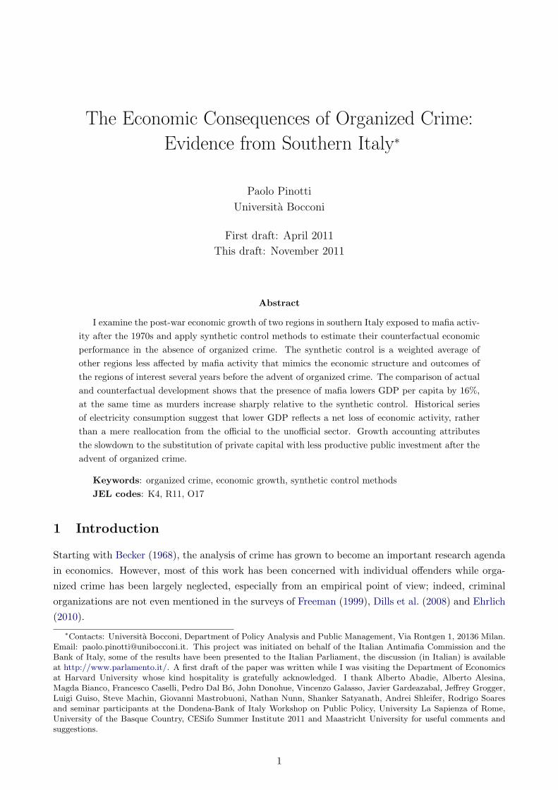
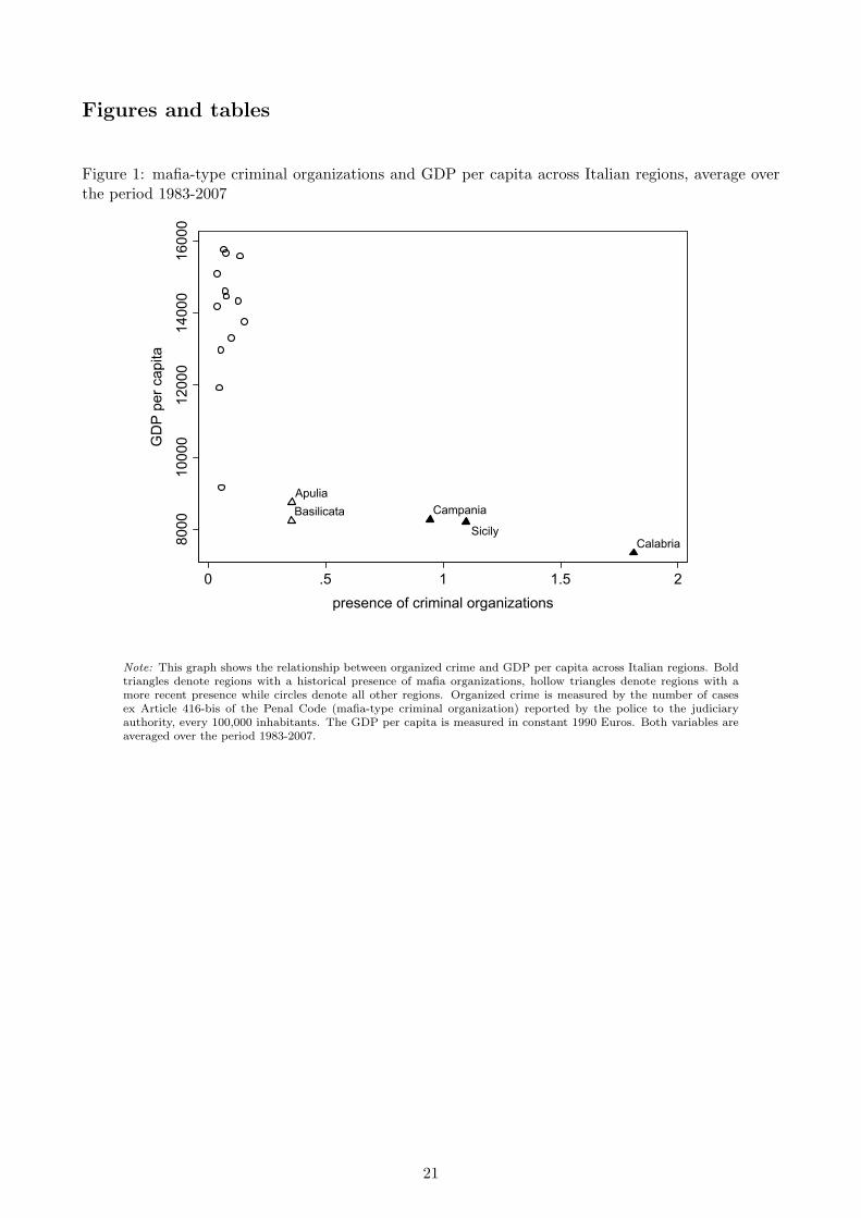
In this paper I empirically investigate the economic consequences of organized crime in Italy duringthe post-war period. Preliminary evidence in Figure 1 suggests that such effects are potentially verylarge; indeed, the five Italian regions where the presence of criminal organizations is more widespreadare also the poorest of the country.2 However, the univariate relationship likely reflects causality goingin both directions. In particular, the level of development could itself be an important factor behindthe rise of criminal organizations.

For this reason, I focus on the peculiar historical experience of Apulia and Basilicata, which suffereda huge increase in the presence of organized crime during the last few decades. Until the beginningof the 1970s, these two regions were in fact characterized by levels of criminal activity and a socialenvironment similar to the other areas of southern Italy not affected by mafia activity. During thefollowing years, however, a series of events largely independent from the socio-economic context ofsuch regions, combined with the expansion of historical mafia organizations beyond their traditionalsettlements in Sicily, Campania and Calabria, resulted in a sudden increase of mafia activity also inApulia and Basilicata.

To address the causal effect of organized crime on economic activity, I thus compare the economicdevelopment of Apulia and Basilicata, before and after the increase in crime, with a control group ofregions not significantly exposed to the presence of criminal organizations. Following the approachoriginally devised by Abadie and Gardeazabal (2003) to estimate the economic costs of terrorism inthe Basque country, I weight units in the control group to construct a synthetic control that mimicsthe initial conditions in Apulia and Basilicata several years before the advent of organized crime. Aslong as the weights reflect some structural parameters that do not vary too much over the mediumperiod, the synthetic control provides a counterfactual scenario for the evolution of the treated regionin the absence of mafia activity.3

1The term “mafia”, originally denoting the specific organization active in Sicily, has been later used to refer to criminalorganizations in general, both inside and outside Italy (see e.g. Gayraud, 2005).

2The measures of organized crime and economic activity are described in great detail in the next sections.3See Abadie et al. (2010) for a throughout presentation of synthetic control methods and Moser (2005), Billmeier and

2

The comparison between the actual and counterfactual scenario shows that the advent of organizedcrime coincides with a sudden slowdown of economic development. Starting from a growth record inline with the other southern regions not significantly exposed to mafia activity, in the course of justa few years around the mid-1970s Apulia and Basilicata move down to an inferior growth path,accumulating an increasing delay over the following decades. Over a thirty-year period, the tworegions experience a 16% drop in GDP per capita relative to the synthetic control, at the same timeas the difference in murder rates increases from 0 to 3 additional homicides per 100,000 inhabitants(twice as much the average murder rate in Italy during the post-war period). Based on a distributionof placebo estimates for all other Italian regions not significantly affected by organized crime, suchchanges in GDP and murders turn out to be extremely unlikely under the null hypothesis of zero effectof organized crime.

In principle, the estimated economic loss may depend on a variety of channels through whichorganized crime affects economic activity. To distinguish among those, I first examine the dynamicsof electricity consumption during the same years as an alternative outcome that depends on economicactivity both in the official and unofficial sector. The evidence in this respect points at an evenlarger drop relative to the synthetic counterfactual, thus excluding that divergence in GDP per capitaafter exposure to mafia activity is explained by a mere reallocation of resources from the official to theunofficial sector. Distinguishing between different components of GDP, sluggish economic performanceseems triggered instead by a strong contraction of private investment in the wake of increasing violencein Apulia and Basilicata, accompanied by a gradual replacement of private with public capital. Thegap accumulated relative to the synthetic counterfactual is then explained by the lower productivityof the latter, documented by several previous studies and confirmed by production function estimatespresented in this paper.

One tentative interpretation of these findings is that criminal organizations discourage productiveinvestment by private entrepreneurs while being able at the same time to secure profit opportunities inpublic procurement. Indeed, according to the Italian judge Giovanni Falcone, who leaded the “MaxiTrial” against the Sicilian mafia in 1987 and was killed by the organization a few years later, “morethan one fifth of Mafia profits come from public investment” (Falcone, 1991).4

This work adds to the literature on the economics of crime. Such literature has produced estimatesof the cost of crime in several countries and through a variety of methods: monetary cost accounting,contingent valuation surveys and willingness-to-pay measures (Soares, 2009, provides a recent review).However, none of these studies has focused explicitly on the costs imposed by the presence of largecriminal organizations. More in general, organized crime has been widely neglected by the empiricalliterature on crime (Fiorentini and Peltzman, 1997).5 The present paper fills this gap employing atransparent data-driven methodology to estimate the economic costs of organized crime in a countrymost plagued by this phenomenon. In this respect, my work is complementary to Acemoglu et al.

Nannicini (2009), Hinrichs (2011) and Montalvo (2011) for recent applications. The surveys of Imbens and Wooldridge(2009) and Lechner (2010) discuss the merits of this approach, while Donald and Lang (2007) and Conley and Taber(2011) propose alternative methods for dealing with small numbers of treated and control units in difference-in-differencemodels.

4According to an extensive anecdotal and judicial evidence, infiltrations in public procurement occur through theintimidation of politicians and public officials. In a companion paper (Pinotti, 2011) I provide additional evidence onthis channel.

5Among the few exceptions, Frye and Zhuravskaya (2000) and Bandiera (2003) estimate the determinants of demandfor private protection in different contexts (Sicily in the XIX century and today’s Russia, respectively), while Mastrobuoniand Patacchini (2010) study the network structure of crime syndicates.

3

(2009), who focus instead on the political consequences of another organization exerting a strongmonopoly of violence outside the control of the state, namely the paramilitaries in Colombia.

The paper is structured as follows. The next Section defines organized crime in the context of theItalian legislative framework and introduces the data that will be used throughout the paper. Then,Section 3 describes in detail the rise of organized crime in Apulia and Basilicata and Section 4 presentsthe identification strategy based on this historical episode. The main empirical results are reportedin Section 5, while Section 6 addresses the potential channels through which organized crime impactson the economy; additional descriptive statistics and robustness exercises are confined to the WebAppendix. Finally, Section 6 concludes.6

2 Organized crime in Italy

2.1 Definitions and legal framework

Criminal organizations are usually involved in a wide range of illegal activities: they supply illicitgoods and services to a variety of consumers; they practice extortion and other predatory activitiesagainst other individuals and firms operating in the economy; finally, they offer private protection incontexts where state enforcement is absent or limited. While there is little disagreement about thesedefining activities, their relative importance has been subject to considerable debate among scholarsand policymakers.

Back in the 1960s, the US Commission on Organized Crime emphasized the role of mobs andgangsters in the provision of “gambling, loan-sharking, narcotics and other forms of vice to countlessnumbers of citizen customers”. According to this view, which is reminiscent of the prohibitionistexperience during the 1930s, “organized crime exists and thrives because it provides services thepublic demands (...) it depends not on victims, but on customers”.

While the above definition points at important aspects of criminal organizations, it neglects on theother hand their core business, namely violence. Far from being a means of last resort, the extensiveuse of violence grants criminal organizations with a strong monopoly power in legal and illegal markets,which they use to extract rents from the other agents in the economy (Schelling, 1971).

Competition over the monopoly of violence may grant criminal organizations with a governancerole also outside the underworld. Indeed, Gambetta (1993) and Skaperdas (2001) argue that the rise ofthe Sicilian Mafia filled a vacuum in the protection of property rights at the dawn of the Italian state.Bandiera (2003) finds empirical support for this hypothesis using historical data on land fragmentationand mafia activity in Sicily at the end of the XIX century.

Criminal organizations in Italy have been traditionally aggressive in exerting the monopoly ofviolence. The pervasive control over the territory allows mafia groups to engage in complex criminalactivities (e.g. smuggling and drug-trafficking) as well as threatening local politicians and publicofficials to influence the allocation of public contracts. The basis of this enormous power rests amongother things on the omerta, which for a long time effectively prevented whistle-blowing by the membersof the organization.7

6The Web Appendix can be downloaded from https://sites.google.com/site/paolopinotti/orgcrime-supplmaterials.7William P. Jennings (1984) includes the enforcement of omerta among the defining activities of criminal organizations.

In Italy, one must wait until 1984 (more than a century after the rise of mafia in Sicily) to have the first importantpentito, Tommaso Buscetta, who described the leadership of the Sicilian Mafia to judge Giovanni Falcone. Acconciaet al. (2009) investigate empirically the effectiveness of leniency programs in Italy, while Spagnolo (2004) and Buccirossi

4

It was only at the beginning of the 1980s that these distinctive features were recognized by theItalian judicial system. Until then, Article 416 of the Penal Code (“associazione a delinquere”)punished in the same way all groups of three or more people involved in some type of criminal activity.Such a generic norm failed thus to distinguish between, say, small groups of bank-robbers and widecriminal networks exerting a ramified control over the territory. This changed in 1982 with Law 646/82,which introduced Article 416-bis (“associazione a delinquere di stampo mafioso”) aimed explicitly atmafia organizations, defined as those groups that “exploit the power of intimidation granted by themembership in the organization and the condition of subjugation and omerta that descends fromit to commit crimes and acquire the control of economic activities, concessions, authorizations andpublic contracts”. Article 416-bis effectively captures the adherence of Italian mafias to the theoreticalframework of Schelling (1971), as well as their interests and infiltrations in the official economy. I nextexamine the distribution of this type of offense across Italian regions.

2.2 Measurement

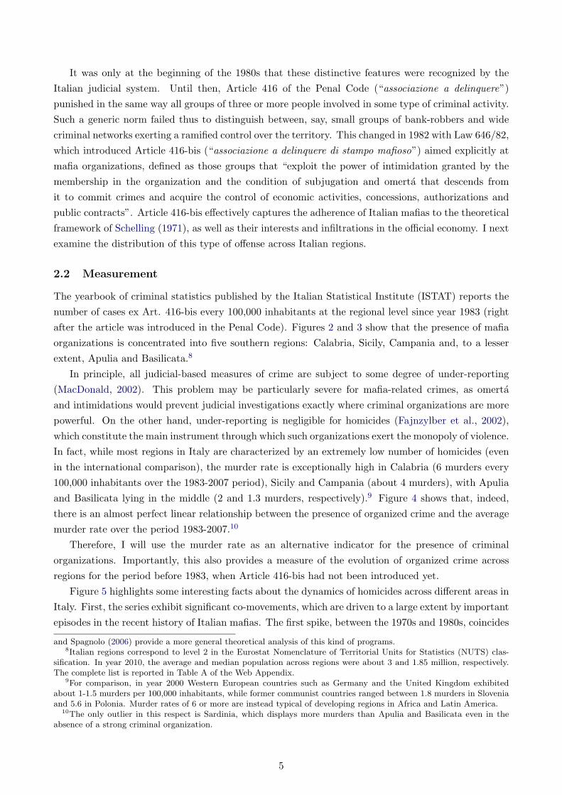
The yearbook of criminal statistics published by the Italian Statistical Institute (ISTAT) reports thenumber of cases ex Art. 416-bis every 100,000 inhabitants at the regional level since year 1983 (rightafter the article was introduced in the Penal Code). Figures 2 and 3 show that the presence of mafiaorganizations is concentrated into five southern regions: Calabria, Sicily, Campania and, to a lesserextent, Apulia and Basilicata.8

In principle, all judicial-based measures of crime are subject to some degree of under-reporting(MacDonald, 2002). This problem may be particularly severe for mafia-related crimes, as omertaand intimidations would prevent judicial investigations exactly where criminal organizations are morepowerful. On the other hand, under-reporting is negligible for homicides (Fajnzylber et al., 2002),which constitute the main instrument through which such organizations exert the monopoly of violence.In fact, while most regions in Italy are characterized by an extremely low number of homicides (evenin the international comparison), the murder rate is exceptionally high in Calabria (6 murders every100,000 inhabitants over the 1983-2007 period), Sicily and Campania (about 4 murders), with Apuliaand Basilicata lying in the middle (2 and 1.3 murders, respectively).9 Figure 4 shows that, indeed,there is an almost perfect linear relationship between the presence of organized crime and the averagemurder rate over the period 1983-2007.10

Therefore, I will use the murder rate as an alternative indicator for the presence of criminalorganizations. Importantly, this also provides a measure of the evolution of organized crime acrossregions for the period before 1983, when Article 416-bis had not been introduced yet.

Figure 5 highlights some interesting facts about the dynamics of homicides across different areas inItaly. First, the series exhibit significant co-movements, which are driven to a large extent by importantepisodes in the recent history of Italian mafias. The first spike, between the 1970s and 1980s, coincides

and Spagnolo (2006) provide a more general theoretical analysis of this kind of programs.8Italian regions correspond to level 2 in the Eurostat Nomenclature of Territorial Units for Statistics (NUTS) clas-

sification. In year 2010, the average and median population across regions were about 3 and 1.85 million, respectively.The complete list is reported in Table A of the Web Appendix.

9For comparison, in year 2000 Western European countries such as Germany and the United Kingdom exhibitedabout 1-1.5 murders per 100,000 inhabitants, while former communist countries ranged between 1.8 murders in Sloveniaand 5.6 in Polonia. Murder rates of 6 or more are instead typical of developing regions in Africa and Latin America.

10The only outlier in this respect is Sardinia, which displays more murders than Apulia and Basilicata even in theabsence of a strong criminal organization.

5

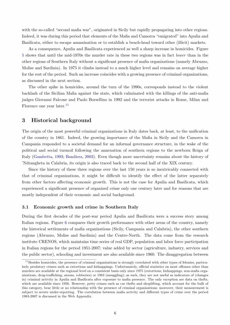
with the so-called “second mafia war”, originated in Sicily but rapidly propagating into other regions.Indeed, it was during this period that elements of the Mafia and Camorra “emigrated” into Apulia andBasilicata, either to escape assassination or to establish a beach-head toward other (illicit) markets.

As a consequence, Apulia and Basilicata experienced as well a sharp increase in homicides. Figure5 shows that until the mid-1970s the murder rate in these two regions was in fact lower than in theother regions of Southern Italy without a significant presence of mafia organizations (namely Abruzzo,Molise and Sardinia). In 1975 it climbs instead to a much higher level and remains on average higherfor the rest of the period. Such an increase coincides with a growing presence of criminal organizations,as discussed in the next section.

The other spike in homicides, around the turn of the 1990s, corresponds instead to the violentbacklash of the Sicilian Mafia against the state, which culminated with the killings of the anti-mafiajudges Giovanni Falcone and Paolo Borsellino in 1992 and the terrorist attacks in Rome, Milan andFlorence one year later.11

3 Historical background

The origin of the most powerful criminal organizations in Italy dates back, at least, to the unificationof the country in 1861. Indeed, the growing importance of the Mafia in Sicily and the Camorra inCampania responded to a societal demand for an informal governance structure, in the wake of thepolitical and social turmoil following the annexation of southern regions to the newborn Reign ofItaly (Gambetta, 1993; Bandiera, 2003). Even though more uncertainty remains about the history of’Ndrangheta in Calabria, its origin is also traced back to the second half of the XIX century.

Since the history of these three regions over the last 150 years is so inextricably connected withthat of criminal organizations, it might be difficult to identify the effect of the latter separatelyfrom other factors affecting economic growth. This is not the case for Apulia and Basilicata, whichexperienced a significant presence of organized crime only one century later and for reasons that aremostly independent of their economic and social background.

3.1 Economic growth and crime in Southern Italy

During the first decades of the post-war period Apulia and Basilicata were a success story amongItalian regions. Figure 6 compares their growth performance with other areas of the country, namelythe historical settlements of mafia organizations (Sicily, Campania and Calabria), the other southernregions (Abruzzo, Molise and Sardinia) and the Centre-North. The data come from the researchinstitute CRENOS, which maintains time series of real GDP, population and labor force participationin Italian regions for the period 1951-2007; value added by sector (agriculture, industry, services andthe public sector), schooling and investment are also available since 1960. The disaggregation between

11Besides homicides, the presence of criminal organizations is strongly correlated with other types of felonies, particu-larly predatory crimes such as extortions and kidnappings. Unfortunately, official statistics on most offenses other thanmurders are available at the regional level on a consistent basis only since 1975 (extortions, kidnappings, non-mafia orga-nizations, drug-trafficking, arsons, robberies) or 1983 (smuggling); as such, they are not useful as indicators of (changesin) criminal activity in Apulia and Basilicata after exposure to mafia presence. The only exception are data on thefts,which are available since 1956. However, petty crimes such as car thefts and shoplifting, which account for the bulk ofthis category, bear little or no relationship with the presence of criminal organizations; moreover, their measurement issubject to severe under-reporting. The correlation between mafia activity and different types of crime over the period1983-2007 is discussed in the Web Appendix.

6

private and public investment, as well as the corresponding capital stocks (reconstructed through theperpetual inventory method) are provided on a consistent basis for the years 1970-1994.12

While the 1960s where characterized by a general convergence between northern and southernsregions, Apulia and Basilicata retained the highest growth rates of the country until the early 1970s,when the process of convergence was over for most other regions (see Paci and Pigliaru, 1997; Terrasi,1999; Maffezzoli, 2006). This scenario changed dramatically over the following decade. Over the courseof just a few years, between the end of the 1970s and the beginning of the 1980s, the growth rate ofthe two regions dropped from being the highest to become the lowest of the country. Historical andjudicial evidence suggests that this period coincides with the outbreak of organized crime in Apuliaand Basilicata, leading to the formation of the so-called fourth and fifth mafia, respectively.

3.2 The rise of organized crime in Apulia and Basilicata

The main source of information on organized crime in Italy are the official records of the Parliamen-tary Antimafia Commission, henceforth PAC, which was first set up in 1962 and renewed in eachsubsequent legislation. The documents most concerned with organized crime in Apulia and Basilicataare those issued between the X and XII legislature of the Italian Parliament (period 1987-1996).13

Secondary sources relying mostly on the PAC reports and other official documents include Ruotolo(1994), Sciarrone (1998), Masciandaro et al. (1999) and Sergi (2003). In general, both primary andsecondary sources agree that the expansion of mafia organizations toward the South-East was pri-marily due to the unfortunate combination of geographic proximity with the historical settlements oforganized crime (Sicily, Campania and Calabria) and a series of events largely independent from thesocio-economic context of the two regions.

The single most important factor explaining the expansion of organized crime toward the south-east is the growing importance of tobacco smuggling during the 1970s (Sciarrone, 1998; PAC, 1993c,p. 11). After the closure of the free port of Tangier in 1960 and the subsequent transfer of tobaccocompanies’ depots into Eastern European countries, the Italian crime syndicates most involved insmuggling abandoned the “Tirrenian route” (from Morocco to Marseilles, through Sicily and Naples)in favor of the “Adriatic route” (from Albania and Yugoslavia toward Turkey and Cyprus, PAC, 2001,p. 10). However, it was only one decade later that mafia organizations expanded beyond the reachof their traditional areas of influence in Sicily, Campania and Calabria. During the 1970s, in fact,smuggling became the most profitable criminal business in Italy, overtaking other illegal activities (suchas gambling, loan-sharking and kidnappings) and anticipating the large-scale trafficking of narcotics,which also followed the same routes. In the words of the former mafia boss Antonino Calderone,“cigarette smuggling was the biggest thing back in the 1970s. It started in the early 1970s and itincreased a lot in 1974-75” (Sciarrone, 1998).

As a consequence, Mafia, Camorra and ’Ndrangheta moved to search for new bases in Apulia,often using Basilicata as a corridor between the Tirrenian and Adriatic coasts. Such traffics receivedan impulse after the collapse of the Eastern Bloc, with the increasing openness to international illegalmarkets by former communist countries on the other side of the Adriatic (PAC, 2001, pp. 46-59).

Another important event leading to an increasing presence of organized crime in Basilicata was12The data set and all related information are publicly available through the website www.crenos.it. They have been

previously used, among others, by Ichino and Maggi (2000) and Tabellini (2010).13Scanned copies of all reports mentioned in the paper (in Italian) can be downloaded from

https://sites.google.com/site/paolopinotti/orgcrime-supplmaterials.

7

the major earthquake that hit the region on November 1980, striking an area of 10,000 square miles atthe border with Campania and Apulia (Sergi, 2003). In the wake of the disaster, the massive amountsof relief money and public investments attracted the interest of criminal organizations. In particular,the absence of a sound legislative and administrative framework for crisis management left local publicadministrations with a great deal of discretion, which in many cases favored widespread mafia infil-trations in procurement contracts (PAC, 1993a). Several judicial investigations and a parliamentarycommission uncovered the embezzlement of a big chunk of the 25 billions of euros allocated for the re-construction, through the intimidation and corruption of local politicians and public administrators.14

Eventually, the main consequence of the flood of public funds was to increase the influence of mafiaorganizations in the regions struck by the earthquake, especially in Basilicata where organized crimehad been almost absent up to that point (PAC, 1993a).

All these events contributed to the breakthrough of organized crime in Apulia and Basilicata. Onefurther element that facilitated its rooting was the presence of several criminals from other regionssent there in confino, a precautionary measure often imposed on individuals that had been eitherconvicted or were strongly suspected of belonging to the mafia. While the purpose of such policywas to break the linkages between criminals and the organization, its main consequence was to favorthe transplantation of mafia into other regions, as recognized in several occasions by the AntimafiaCommission (e.g. PAC, 1994). It turns out that, between 1961 and 1972 (official records for subsequentyears have been destroyed), Apulia was the southern region hosting the greatest number of criminalsin confino, while in Basilicata their number was particularly high relative to the initial population(Tranfaglia, 2008). Also, during the 1970s the two regions received several prison inmates transferredfrom Campania, in order to avoid fights in jail between opposing factions of the Camorra. Subsequentjudiciary investigations proved that these individuals constituted an important link with the criminalorganizations of other regions (PAC, 1991, pp. 52-53).

At the beginning, illegal activities in Apulia and Basilicata were conducted directly by Mafia,Camorra and ’Ndrangheta, exploiting local criminal workforce in exchange for protection and financialresources. Such an arrangement proved unstable, as very soon local groups acquired independence byorganizing themselves into autonomous crime syndicates, the most important of which are the SacraCorona Unita in Apulia and the Basilischi in Basilicata.

4 Empirical methodology

The previous section described how the rise and expansion of organized crime in Apulia and Basilicata,between the end of the 1970s and the beginning of the 1980s, was largely driven by factors independentfrom the economic and social context of these two regions, namely the switch of smugglers towardeastern routes, the political turmoil in eastern European countries and the earthquake of 1980. Theempirical strategy adopted in this paper exploits this historical change to estimate the effect of orga-nized crime by comparing Apulia and Basilicata with a control group of regions not (or less) affectedby organized crime. To reduce the scope for omitted variable bias, I follow the approach of Abadieand Gardeazabal (2003) and Abadie et al. (2010), weighting units in the control group to construct asynthetic counterfactual that replicates the initial conditions and the growth potential of the regions

14Less than a month after the disaster, the mayor of a town in Campania was killed for refusing to award the contractfor clearing the detritus to a company connected with the Camorra. Similar episodes recurred frequently over thefollowing years.

8

of interest before exposure to mafia presence.

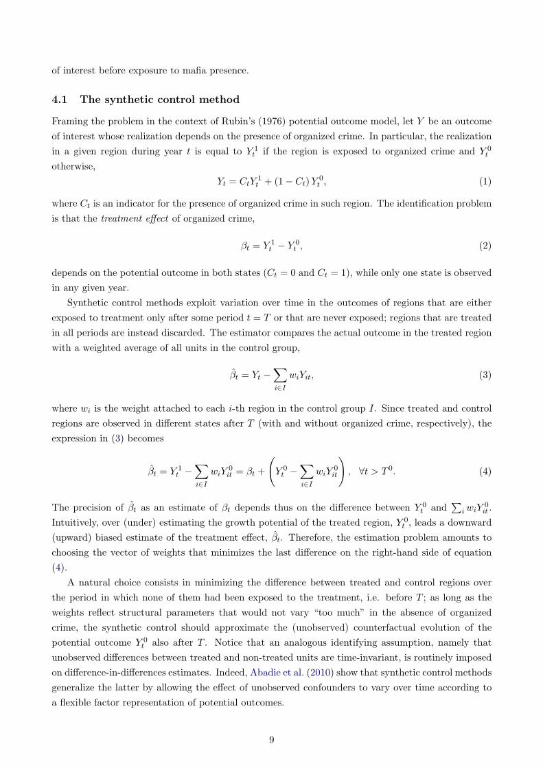
4.1 The synthetic control method

Framing the problem in the context of Rubin’s (1976) potential outcome model, let Y be an outcomeof interest whose realization depends on the presence of organized crime. In particular, the realizationin a given region during year t is equal to Y 1

t if the region is exposed to organized crime and Y 0t

otherwise,Yt = CtY

1t + (1− Ct)Y 0

t , (1)

where Ct is an indicator for the presence of organized crime in such region. The identification problemis that the treatment effect of organized crime,

βt = Y 1t − Y 0

t , (2)

depends on the potential outcome in both states (Ct = 0 and Ct = 1), while only one state is observedin any given year.

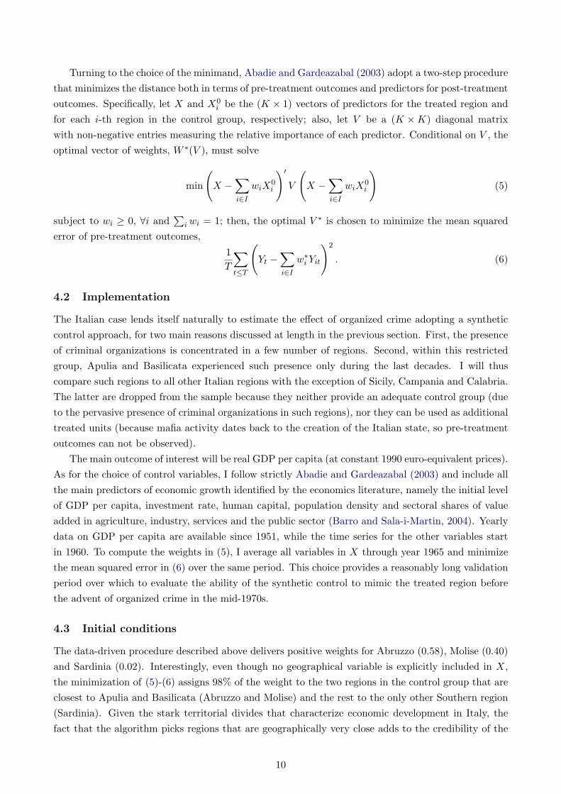
Synthetic control methods exploit variation over time in the outcomes of regions that are eitherexposed to treatment only after some period t = T or that are never exposed; regions that are treatedin all periods are instead discarded. The estimator compares the actual outcome in the treated regionwith a weighted average of all units in the control group,

βt = Yt −∑i∈I

wiYit, (3)

where wi is the weight attached to each i-th region in the control group I. Since treated and controlregions are observed in different states after T (with and without organized crime, respectively), theexpression in (3) becomes

βt = Y 1t −

∑i∈I

wiY0it = βt +

(Y 0

t −∑i∈I

wiY0it

), ∀t > T 0. (4)

The precision of βt as an estimate of βt depends thus on the difference between Y 0t and

∑iwiY

0it .

Intuitively, over (under) estimating the growth potential of the treated region, Y 0t , leads a downward

(upward) biased estimate of the treatment effect, βt. Therefore, the estimation problem amounts tochoosing the vector of weights that minimizes the last difference on the right-hand side of equation(4).

A natural choice consists in minimizing the difference between treated and control regions overthe period in which none of them had been exposed to the treatment, i.e. before T ; as long as theweights reflect structural parameters that would not vary “too much” in the absence of organizedcrime, the synthetic control should approximate the (unobserved) counterfactual evolution of thepotential outcome Y 0

t also after T . Notice that an analogous identifying assumption, namely thatunobserved differences between treated and non-treated units are time-invariant, is routinely imposedon difference-in-differences estimates. Indeed, Abadie et al. (2010) show that synthetic control methodsgeneralize the latter by allowing the effect of unobserved confounders to vary over time according toa flexible factor representation of potential outcomes.

9

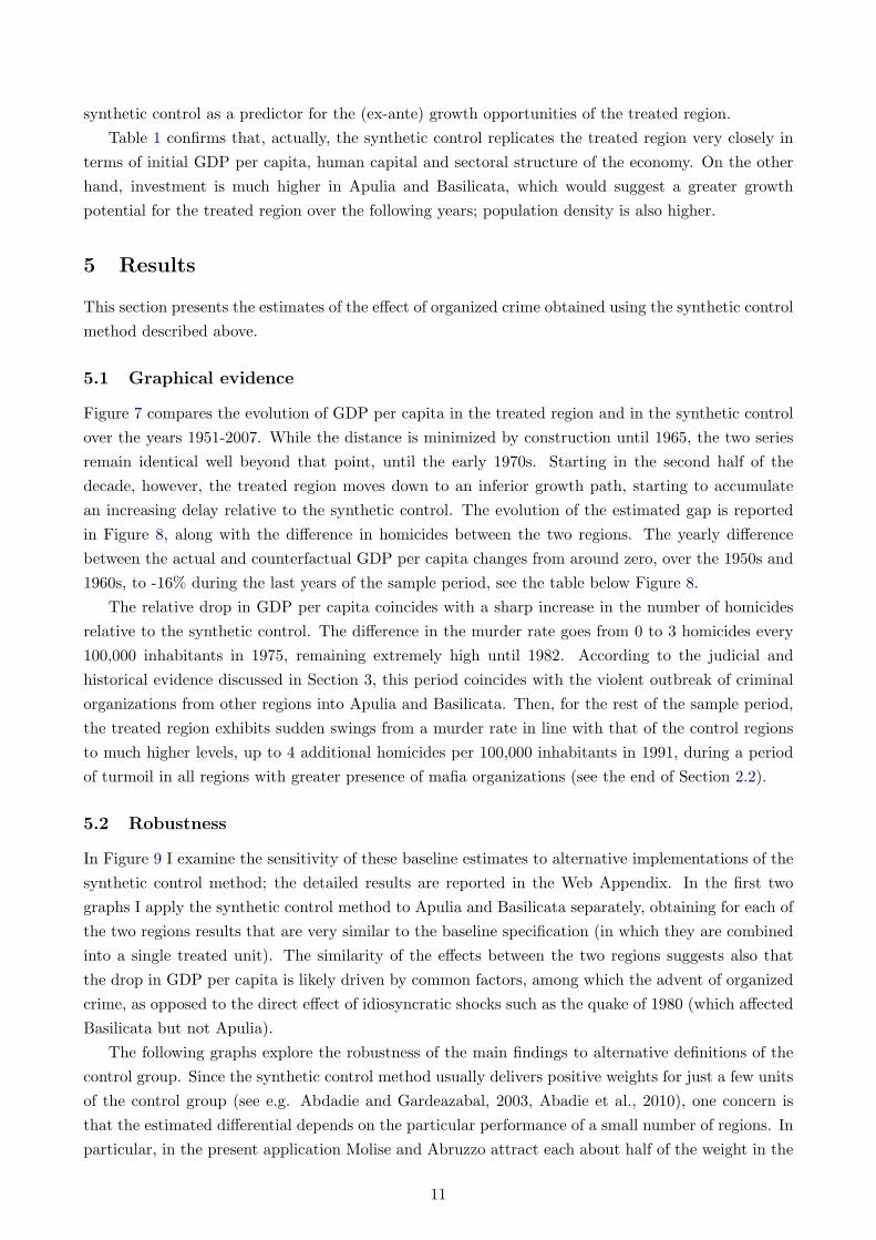
Turning to the choice of the minimand, Abadie and Gardeazabal (2003) adopt a two-step procedurethat minimizes the distance both in terms of pre-treatment outcomes and predictors for post-treatmentoutcomes. Specifically, let X and X0

i be the (K × 1) vectors of predictors for the treated region andfor each i-th region in the control group, respectively; also, let V be a (K ×K) diagonal matrixwith non-negative entries measuring the relative importance of each predictor. Conditional on V , theoptimal vector of weights, W ∗(V ), must solve

min

(X −

∑i∈I

wiX0i

)′V

(X −

∑i∈I

wiX0i

)(5)

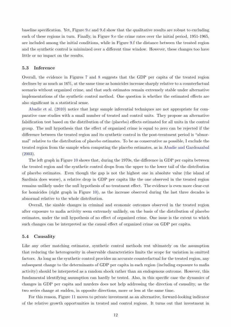
subject to wi ≥ 0, ∀i and∑

iwi = 1; then, the optimal V ∗ is chosen to minimize the mean squarederror of pre-treatment outcomes,

1T

∑t≤T

(Yt −

∑i∈I

w∗i Yit

)2

. (6)

4.2 Implementation

The Italian case lends itself naturally to estimate the effect of organized crime adopting a syntheticcontrol approach, for two main reasons discussed at length in the previous section. First, the presenceof criminal organizations is concentrated in a few number of regions. Second, within this restrictedgroup, Apulia and Basilicata experienced such presence only during the last decades. I will thuscompare such regions to all other Italian regions with the exception of Sicily, Campania and Calabria.The latter are dropped from the sample because they neither provide an adequate control group (dueto the pervasive presence of criminal organizations in such regions), nor they can be used as additionaltreated units (because mafia activity dates back to the creation of the Italian state, so pre-treatmentoutcomes can not be observed).

The main outcome of interest will be real GDP per capita (at constant 1990 euro-equivalent prices).As for the choice of control variables, I follow strictly Abadie and Gardeazabal (2003) and include allthe main predictors of economic growth identified by the economics literature, namely the initial levelof GDP per capita, investment rate, human capital, population density and sectoral shares of valueadded in agriculture, industry, services and the public sector (Barro and Sala-i-Martin, 2004). Yearlydata on GDP per capita are available since 1951, while the time series for the other variables startin 1960. To compute the weights in (5), I average all variables in X through year 1965 and minimizethe mean squared error in (6) over the same period. This choice provides a reasonably long validationperiod over which to evaluate the ability of the synthetic control to mimic the treated region beforethe advent of organized crime in the mid-1970s.

4.3 Initial conditions

The data-driven procedure described above delivers positive weights for Abruzzo (0.58), Molise (0.40)and Sardinia (0.02). Interestingly, even though no geographical variable is explicitly included in X,the minimization of (5)-(6) assigns 98% of the weight to the two regions in the control group that areclosest to Apulia and Basilicata (Abruzzo and Molise) and the rest to the only other Southern region(Sardinia). Given the stark territorial divides that characterize economic development in Italy, thefact that the algorithm picks regions that are geographically very close adds to the credibility of the

10

synthetic control as a predictor for the (ex-ante) growth opportunities of the treated region.Table 1 confirms that, actually, the synthetic control replicates the treated region very closely in

terms of initial GDP per capita, human capital and sectoral structure of the economy. On the otherhand, investment is much higher in Apulia and Basilicata, which would suggest a greater growthpotential for the treated region over the following years; population density is also higher.

5 Results

This section presents the estimates of the effect of organized crime obtained using the synthetic controlmethod described above.

5.1 Graphical evidence

Figure 7 compares the evolution of GDP per capita in the treated region and in the synthetic controlover the years 1951-2007. While the distance is minimized by construction until 1965, the two seriesremain identical well beyond that point, until the early 1970s. Starting in the second half of thedecade, however, the treated region moves down to an inferior growth path, starting to accumulatean increasing delay relative to the synthetic control. The evolution of the estimated gap is reportedin Figure 8, along with the difference in homicides between the two regions. The yearly differencebetween the actual and counterfactual GDP per capita changes from around zero, over the 1950s and1960s, to -16% during the last years of the sample period, see the table below Figure 8.

The relative drop in GDP per capita coincides with a sharp increase in the number of homicidesrelative to the synthetic control. The difference in the murder rate goes from 0 to 3 homicides every100,000 inhabitants in 1975, remaining extremely high until 1982. According to the judicial andhistorical evidence discussed in Section 3, this period coincides with the violent outbreak of criminalorganizations from other regions into Apulia and Basilicata. Then, for the rest of the sample period,the treated region exhibits sudden swings from a murder rate in line with that of the control regionsto much higher levels, up to 4 additional homicides per 100,000 inhabitants in 1991, during a periodof turmoil in all regions with greater presence of mafia organizations (see the end of Section 2.2).

5.2 Robustness

In Figure 9 I examine the sensitivity of these baseline estimates to alternative implementations of thesynthetic control method; the detailed results are reported in the Web Appendix. In the first twographs I apply the synthetic control method to Apulia and Basilicata separately, obtaining for each ofthe two regions results that are very similar to the baseline specification (in which they are combinedinto a single treated unit). The similarity of the effects between the two regions suggests also thatthe drop in GDP per capita is likely driven by common factors, among which the advent of organizedcrime, as opposed to the direct effect of idiosyncratic shocks such as the quake of 1980 (which affectedBasilicata but not Apulia).

The following graphs explore the robustness of the main findings to alternative definitions of thecontrol group. Since the synthetic control method usually delivers positive weights for just a few unitsof the control group (see e.g. Abdadie and Gardeazabal, 2003, Abadie et al., 2010), one concern isthat the estimated differential depends on the particular performance of a small number of regions. Inparticular, in the present application Molise and Abruzzo attract each about half of the weight in the

11

baseline specification. Yet, Figure 9.c and 9.d show that the qualitative results are robust to excludingeach of these regions in turn. Finally, in Figure 9.e the crime rates over the initial period, 1951-1965,are included among the initial conditions, while in Figure 9.f the distance between the treated regionand the synthetic control is minimized over a different time window. However, these changes too havelittle or no impact on the results.

5.3 Inference

Overall, the evidence in Figures 7 and 8 suggests that the GDP per capita of the treated regiondeclines by as much as 16%, at the same time as homicides increase sharply relative to a counterfactualscenario without organized crime, and that such estimates remain extremely stable under alternativeimplementations of the synthetic control method. One question is whether the estimated effects arealso significant in a statistical sense.

Abadie et al. (2010) notice that large sample inferential techniques are not appropriate for com-parative case studies with a small number of treated and control units. They propose an alternativefalsification test based on the distribution of the (placebo) effects estimated for all units in the controlgroup. The null hypothesis that the effect of organized crime is equal to zero can be rejected if thedifference between the treated region and its synthetic control in the post-treatment period is “abnor-mal” relative to the distribution of placebo estimates. To be as conservative as possible, I exclude thetreated region from the sample when computing the placebo estimates, as in Abadie and Gardeazabal(2003).

The left graph in Figure 10 shows that, during the 1970s, the difference in GDP per capita betweenthe treated region and the synthetic control drops from the upper to the lower tail of the distributionof placebo estimates. Even though the gap is not the highest one in absolute value (the island ofSardinia does worse), a relative drop in GDP per capita like the one observed in the treated regionremains unlikely under the null hypothesis of no treatment effect. The evidence is even more clear-cutfor homicides (right graph in Figure 10), as the increase observed during the last three decades isabnormal relative to the whole distribution.

Overall, the sizable changes in criminal and economic outcomes observed in the treated regionafter exposure to mafia activity seem extremely unlikely, on the basis of the distribution of placeboestimates, under the null hypothesis of no effect of organized crime. One issue is the extent to whichsuch changes can be interpreted as the causal effect of organized crime on GDP per capita.

5.4 Causality

Like any other matching estimator, synthetic control methods rest ultimately on the assumptionthat reducing the heterogeneity in observable characteristics limits the scope for variation in omittedfactors. As long as the synthetic control provides an accurate counterfactual for the treated region, anysubsequent change to the determinants of GDP per capita in each region (including exposure to mafiaactivity) should be interpreted as a random shock rather than an endogenous outcome. However, thisfundamental identifying assumption can hardly be tested. Also, in this specific case the dynamics ofchanges in GDP per capita and murders does not help addressing the direction of causality, as thetwo series change at sudden, in opposite directions, more or less at the same time.

For this reason, Figure 11 moves to private investment as an alternative, forward-looking indicatorof the relative growth opportunities in treated and control regions. It turns out that investment in

12

Apulia and Basilicata remained sustained until the breakthrough of violence and declined only a coupleof years later. Therefore, there is no indication that the two regions were experiencing a change inthe economic outlook before (or at the same time of) the advent of organized crime.

To address causality in a more systematic way, I employ regression analysis and exploit changes incriminal activity in the regions with historical mafia presence excluded from the control group (Sicily,Campania and Calabria) as a source of variation in the intensity of mafia activity in Apulia andBasilicata. As shown in Figure 5, the dynamics of homicides across Italian regions exhibits significantco-movements induced by major events in the recent history of the Sicilian Mafia (see the end of Section2.2). As long as such events depend only to a minor extent, if at all, on the economic developmentof Apulia and Basilicata relative to the synthetic control, it is possible to estimate the effect of mafiaactivity in a Two-Stage Least Squares (2SLS) framework.

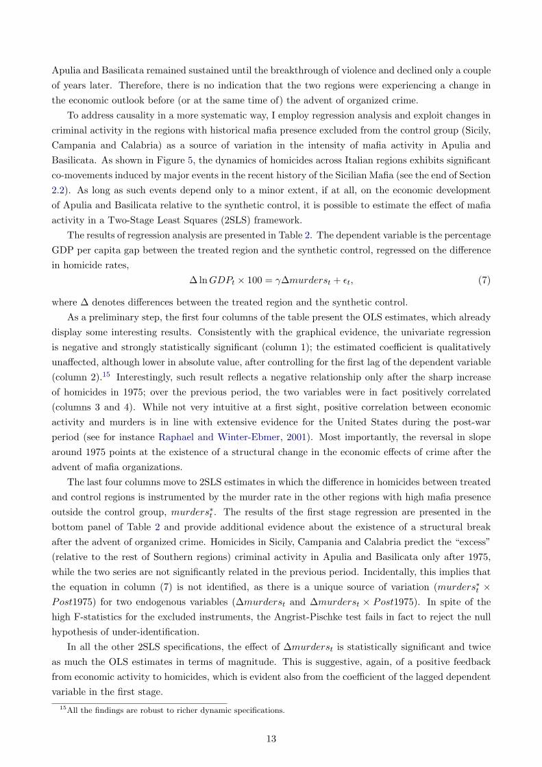
The results of regression analysis are presented in Table 2. The dependent variable is the percentageGDP per capita gap between the treated region and the synthetic control, regressed on the differencein homicide rates,

∆ lnGDPt × 100 = γ∆murderst + εt, (7)

where ∆ denotes differences between the treated region and the synthetic control.As a preliminary step, the first four columns of the table present the OLS estimates, which already

display some interesting results. Consistently with the graphical evidence, the univariate regressionis negative and strongly statistically significant (column 1); the estimated coefficient is qualitativelyunaffected, although lower in absolute value, after controlling for the first lag of the dependent variable(column 2).15 Interestingly, such result reflects a negative relationship only after the sharp increaseof homicides in 1975; over the previous period, the two variables were in fact positively correlated(columns 3 and 4). While not very intuitive at a first sight, positive correlation between economicactivity and murders is in line with extensive evidence for the United States during the post-warperiod (see for instance Raphael and Winter-Ebmer, 2001). Most importantly, the reversal in slopearound 1975 points at the existence of a structural change in the economic effects of crime after theadvent of mafia organizations.

The last four columns move to 2SLS estimates in which the difference in homicides between treatedand control regions is instrumented by the murder rate in the other regions with high mafia presenceoutside the control group, murders∗t . The results of the first stage regression are presented in thebottom panel of Table 2 and provide additional evidence about the existence of a structural breakafter the advent of organized crime. Homicides in Sicily, Campania and Calabria predict the “excess”(relative to the rest of Southern regions) criminal activity in Apulia and Basilicata only after 1975,while the two series are not significantly related in the previous period. Incidentally, this implies thatthe equation in column (7) is not identified, as there is a unique source of variation (murders∗t ×Post1975) for two endogenous variables (∆murderst and ∆murderst × Post1975). In spite of thehigh F-statistics for the excluded instruments, the Angrist-Pischke test fails in fact to reject the nullhypothesis of under-identification.

In all the other 2SLS specifications, the effect of ∆murderst is statistically significant and twiceas much the OLS estimates in terms of magnitude. This is suggestive, again, of a positive feedbackfrom economic activity to homicides, which is evident also from the coefficient of the lagged dependentvariable in the first stage.

15All the findings are robust to richer dynamic specifications.

13

Such results must be taken with caution, as the exclusion restriction behind 2SLS estimates couldbe invalidated by direct effects of criminal activity in Sicily, Campania and Calabria on the GDP percapita of the treated regions through channels other than criminal activity in the latter. Still, thedependent variable is the differential economic performance of treated and control regions, which areall located at similar distance from the high-mafia regions, so it is not clear why spillover effects shouldbe asymmetric between treated and control units. More in general, the results in Table 2 seem at leastsuggestive of the existence of positive reverse causality effects, from greater growth opportunities tohigher mafia presence. If this is the case, the synthetic control estimate would provide a lower boundfor the economic costs of organized crime.

6 Channels

The results presented so far suggest that organized crime has a strong, negative effect on economicgrowth and development; yet, they are silent about the mechanisms behind such effect. In thissection I thus provide additional empirical evidence that helps distinguishing between a few alternativeexplanations.

6.1 Official and unofficial economy

One possible interpretation of the divergence between the treated region and the synthetic control isthat the presence of criminal organizations changes the relative importance of the official sector, asmeasured by GDP per capita, vis-a-vis the shadow economy. Additional employment opportunities inthe unofficial sector could lead in fact to a reallocation of workers and resources outside the scope ofofficial statistics. Under this alternative explanation, the differential in official GDP per capita wouldover-estimate the change in welfare after exposure to mafia activity as lower GDP per capita wouldjust reflect a different composition (but not a different level) of economic activity.

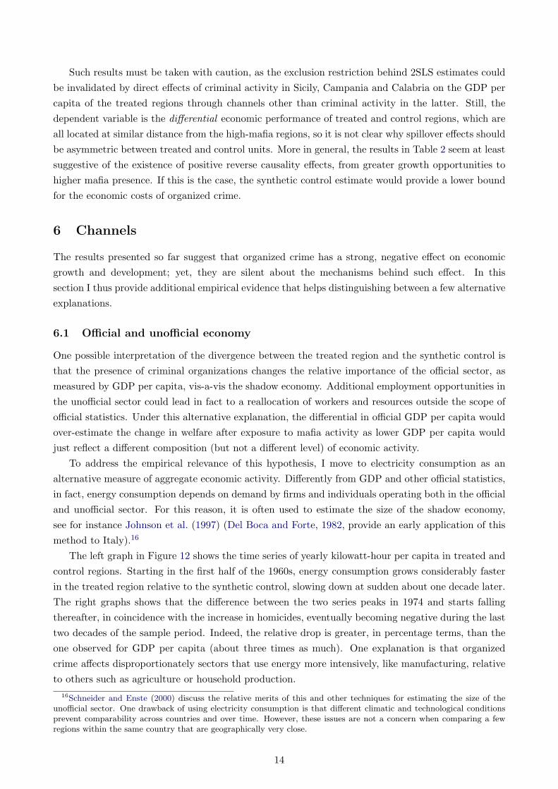
To address the empirical relevance of this hypothesis, I move to electricity consumption as analternative measure of aggregate economic activity. Differently from GDP and other official statistics,in fact, energy consumption depends on demand by firms and individuals operating both in the officialand unofficial sector. For this reason, it is often used to estimate the size of the shadow economy,see for instance Johnson et al. (1997) (Del Boca and Forte, 1982, provide an early application of thismethod to Italy).16

The left graph in Figure 12 shows the time series of yearly kilowatt-hour per capita in treated andcontrol regions. Starting in the first half of the 1960s, energy consumption grows considerably fasterin the treated region relative to the synthetic control, slowing down at sudden about one decade later.The right graphs shows that the difference between the two series peaks in 1974 and starts fallingthereafter, in coincidence with the increase in homicides, eventually becoming negative during the lasttwo decades of the sample period. Indeed, the relative drop is greater, in percentage terms, than theone observed for GDP per capita (about three times as much). One explanation is that organizedcrime affects disproportionately sectors that use energy more intensively, like manufacturing, relativeto others such as agriculture or household production.

16Schneider and Enste (2000) discuss the relative merits of this and other techniques for estimating the size of theunofficial sector. One drawback of using electricity consumption is that different climatic and technological conditionsprevent comparability across countries and over time. However, these issues are not a concern when comparing a fewregions within the same country that are geographically very close.

14

In any case, there is no evidence that the slowdown in the official sector was compensated for byan expansion of the shadow economy. Therefore, the 16% reduction in GDP per capita correspondsto an analogous (or even greater) aggregate economic loss in the treated region.

6.2 Growth accounting

In order to better understand the channels through which organized crime impacts on GDP percapita, I perform a simple growth accounting exercise, decomposing the gap between treated andcontrol regions into differences in factor accumulation and productivity. I stick to the workhorsemodel adopted in the growth accounting literature, namely the Cobb-Douglas production functionwith constant returns to scale in capital and labor (see e.g. Barro, 1999),

lnYt = lnAt + αL lnLt + (1− αL) lnKt, (8)

where αL is the labor share, L and K are labor and capital inputs, respectively, and A is total factorproductivity. The growth differential between treated and control regions is given by the weightedsum of the growth differential for these three components,

∆(lnYt − lnYt−1) = ∆(lnAt − lnAt−1) + αL∆(lnLt − lnLt−1) + (1− αL)∆(lnKt − lnKt−1),

where ∆ denotes again differentials between the treated region and the synthetic control.For the period 1970-1994 the dataset CRENOS reports consistent time series of regional labor

workforce and capital stock, reconstructed through the perpetual inventory method; fixing the laborshare, one can back up total factor productivity as a residual.

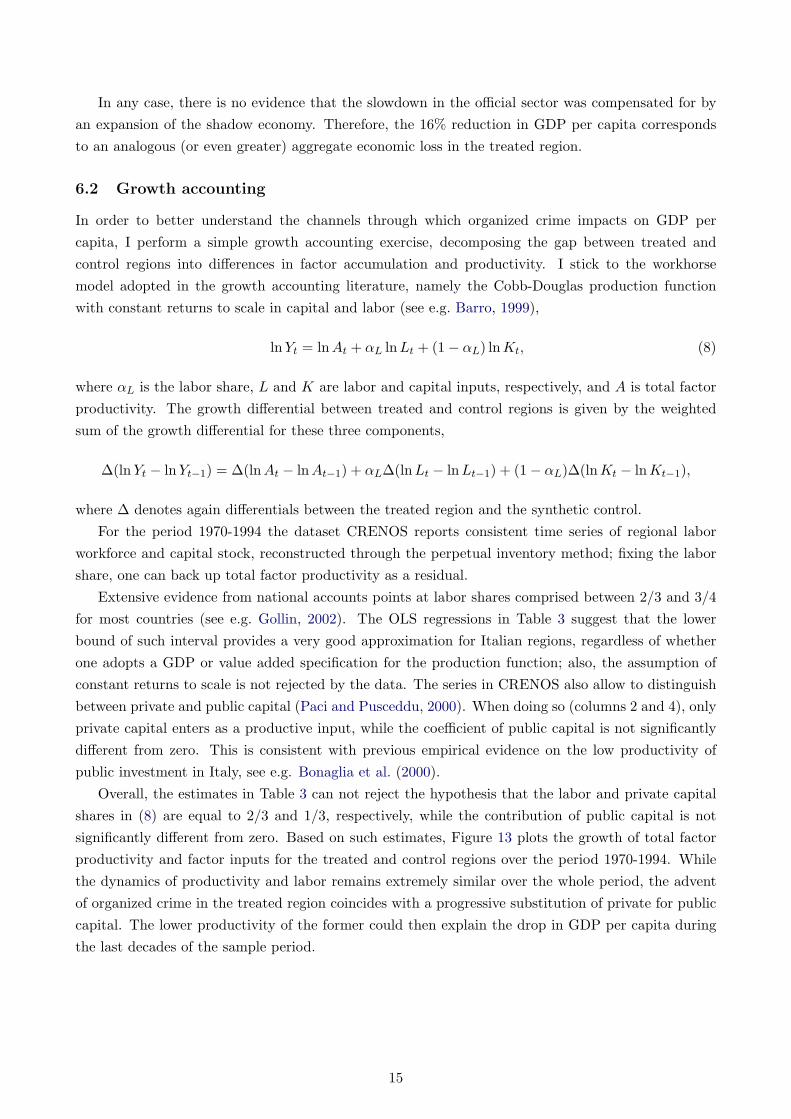
Extensive evidence from national accounts points at labor shares comprised between 2/3 and 3/4for most countries (see e.g. Gollin, 2002). The OLS regressions in Table 3 suggest that the lowerbound of such interval provides a very good approximation for Italian regions, regardless of whetherone adopts a GDP or value added specification for the production function; also, the assumption ofconstant returns to scale is not rejected by the data. The series in CRENOS also allow to distinguishbetween private and public capital (Paci and Pusceddu, 2000). When doing so (columns 2 and 4), onlyprivate capital enters as a productive input, while the coefficient of public capital is not significantlydifferent from zero. This is consistent with previous empirical evidence on the low productivity ofpublic investment in Italy, see e.g. Bonaglia et al. (2000).

Overall, the estimates in Table 3 can not reject the hypothesis that the labor and private capitalshares in (8) are equal to 2/3 and 1/3, respectively, while the contribution of public capital is notsignificantly different from zero. Based on such estimates, Figure 13 plots the growth of total factorproductivity and factor inputs for the treated and control regions over the period 1970-1994. Whilethe dynamics of productivity and labor remains extremely similar over the whole period, the adventof organized crime in the treated region coincides with a progressive substitution of private for publiccapital. The lower productivity of the former could then explain the drop in GDP per capita duringthe last decades of the sample period.

15

6.3 Discussion of the results

According to the growth accounting exercise, public intervention takes over an increasing share ofeconomic activity after the presence of criminal organizations hampers private investment. One ex-planation for this pattern could be that the central government and local public administrations useemployment in the public sector to cushion the drop in labor market opportunities after the with-drawal of private investors. However, the last two graphs in Figure 13 show that the replacement ofprivate with public capital is not accompanied by an analogous reallocation in the labor market.

A less benevolent explanation is that public money represents a profit opportunity for criminalorganizations. For instance, mafia rackets often force firms to purchase over-priced inputs or hireindividuals that are close to the organization. Such practices levitate production costs and are thereforeeasier to impose on firms that may offload such costs or are somehow shielded from market competition(Schelling, 1971); contractors for public works fit perfectly into these categories. Also, firms connectedwith the mafia may adjudicate directly public contracts by threatening the other potential bidders inprocurement auctions.17

For all these reasons, criminal organizations in Italy may want to attract public investment towardtheir areas of influence. To this purpose, they do not hesitate to corrupt and/or threaten politiciansand public officials (PAC, 1993b,a), which in turn affects the selection of the ruling class. Dal Bo et al.(2006) argue in fact that the personal risks to which public officials are exposed in the areas mostpervaded by criminal organizations may discourage individuals with better outside opportunities fromentering a political career. While a throughout analysis of the influence of organized crime on thepolitical sphere goes beyond the scope of the present work, in a companion paper I document indeeda strong deterioration in the outside labor market opportunities of the politicians appointed in Apuliaand Basilicata (relative to the synthetic control) after the advent of organized crime (Pinotti, 2011).

Therefore, a tentative interpretation for the increase in public expenditure observed during thesame period is that, amidst greater violence and worse economic prospects, local politicians were“captured” by criminal organizations. Such interpretation would also be consistent with recent workby Acemoglu et al. (2009) on Colombian politicians appointed in the areas most exposed to the activityof paramilitary groups.

7 Conclusion

The present study provides the first available evidence on the economic costs of organized crime. Theempirical exercise applies a transparent and intuitive policy evaluation method, originally devisedby Abadie and Gardeazabal (2003), to study the economic effects of organized crime in two Italianregions recently exposed to this phenomenon. The results suggest that the aggregate loss impliedby the presence of organized crime amounts to 16% of GDP per capita and goes mainly through areallocation from private economic activity to (less productive) public investment.

One limitation of the macroeconomic approach adopted here is that it does not lend itself easilyto explore these mechanisms in greater detail. Another limit concerns the external validity of theestimates, which is constrained by the specificities of a complex phenomenon such as organized crimein different countries and periods. Finally, the outcomes examined here (primarily GDP per capita

17See Caneppele et al. (2009) for a systematic discussion of the methods used by criminal organizations to infiltratepublic contracts. Reuter (1987) provides an interesting case study for the garbage collection industry in New York.

16

and its components) capture only some of the effects of organized crime on social welfare. Utilitylosses along many other dimensions (human, psychological and social) have no direct counterpart intoobservable quantities, even though indicators such as life expectancy and housing prices may go a longway in this direction (see, respectively, Thaler, 1978; Soares, 2006).

For all these reasons, the present study should be seen as a first step to better understand theeconomic effects of organized crime, as well as an indication that such effects might be large enoughto deserve further attention in the future.

References

Abadie, A., A. Diamond, and J. Hainmueller (2010). Synthetic control methods for comparative casestudies: Estimating the effect of california’s tobacco control program. Journal of the AmericanStatistical Association 105 (490), 493–505.

Abadie, A. and J. Gardeazabal (2003). The economic costs of conflict: A case study of the basquecountry. The American Economic Review 93 (1), pp. 113–132.

Acconcia, A., G. Immordino, S. Piccolo, and P. Rey (2009). Accomplice-witnesses, organized crimeand corruption: Theory and evidence from italy. Technical report.

Acemoglu, D., J. A. Robinson, and R. Santos (2009). The monopoly of violence: Evidence fromcolombia. Technical report.

Bandiera, O. (2003). Land reform, the market for protection, and the origins of the sicilian mafia:Theory and evidence. Journal of Law, Economics and Organization 19 (1), 218–244.

Barro, R. and X. Sala-i-Martin (2004). Economic Growth. MIT Press.

Barro, R. J. (1999). Notes on growth accounting. Journal of Economic Growth 4 (2), 119–37.

Becker, G. S. (1968). Crime and punishment: An economic approach. The Journal of PoliticalEconomy 76 (2), pp. 169–217.

Billmeier, A. and T. Nannicini (2009). Trade openness and growth: Pursuing empirical glasnost. IMFStaff Papers 56 (3), 447–475.

Bonaglia, F., E. L. Ferrara, and M. Marcellino (2000). Public capital and economic performance:Evidence from italy. Giornale degli Economisti 59 (2), 221–244.

Buccirossi, P. and G. Spagnolo (2006). Leniency policies and illegal transactions. Journal of PublicEconomics 90 (6-7), 1281 – 1297.

Caneppele, S., F. Calderoni, and S. Martocchia (2009). Not only banks: Criminological modelson the infiltration of public contracts by Italian organized crime. Journal of Money LaunderingControl 12 (2), 151–172.

Conley, T. G. and C. R. Taber (2011). Inference with difference in differences with a small number ofpolicy changes. Review of Economics and Statistics 93 (1), 113–125.

17

Dal Bo, E., P. Dal Bo, and R. Di Tella (2006). Plata o plomo: Bribe and punishment in a theory ofpolitical influence. American Political Science Review 100 (1), 41–53.

Del Boca, D. and F. Forte (1982). Recent empirical surveys and theoretical interpretations of theparallel economy in italy. In V. Tanzi (Ed.), The Underground Economy in the United States andAbroad. Lexington: D.C. Heath.

Dills, A. K., J. A. Miron, and G. Summers (2008). What do economists know about crime? WorkingPaper 13759, National Bureau of Economic Research.

Donald, S. G. and K. Lang (2007). Inference with difference-in-differences and other panel data. TheReview of Economics and Statistics 89 (2), 221–233.

Ehrlich, I. (2010). The market model of crime: a short review and new directions. In B. L. Bensonand P. R. Zimmerman (Eds.), Handbook on the Economics of Crime. Elsevier.

Fajnzylber, P., D. Lederman, and N. Loayza (2002). What causes violent crime? European EconomicReview 46 (7), 1323–1357.

Falcone, G. (1991). Cose di Cosa Nostra. Biblioteca Universale Rizzoli.

Fiorentini, G. and S. Peltzman (1997). Introduction. In G. Fiorentini and S. Peltzman (Eds.), TheEconomics of Organised Crime. Cambridge University Press.

Freeman, R. B. (1999). The economics of crime. In O. Ashenfelter and D. Card (Eds.), Handbook ofLabor Economics. Elsevier.

Frye, T. and E. Zhuravskaya (2000). Rackets, regulation, and the rule of law. Journal of Law,Economics and Organization 16 (2), 478–502.

Gambetta, D. (1993). The Sicilian Mafia: the business of private protection. Harvard UniversityPress.

Gayraud, J.-F. (2005). Le monde des mafias. Editions Odile Jacob.

Gollin, D. (2002). Getting income shares right. The Journal of Political Economy 110 (2), pp. 458–474.

Hinrichs, P. (2011). The effects of affirmative action bans on college enrollment, educational at-tainment, and the demographic composition of universities. Review of Economics and Statistics(forthcoming).

Ichino, A. and G. Maggi (2000). Work environment and individual background: Explaining regionalshirking differentials in a large italian firm. The Quarterly Journal of Economics 115 (3), pp. 1057–1090.

Imbens, G. W. and J. M. Wooldridge (2009). Recent developments in the econometrics of programevaluation. Journal of Economic Literature 47 (1), 5–86.

Johnson, S., D. Kaufmann, and A. Shleifer (1997). The unofficial economy in transition. BrookingsPapers on Economic Activity 1997 (2), pp. 159–239.

18

Lechner, M. (2010). The estimation of causal effects by difference-in-difference methods. Technicalreport.

MacDonald, Z. (2002). Official crime statistics: Their use and interpretation. Economic Jour-nal 112 (477), F85–F106.

Maffezzoli, M. (2006). Convergence across italian regions and the role of technological catch-up. TheB.E. Journal of Macroeconomics 0 (1).

Masciandaro, D., F. Roberti, and P. L. Vigna (1999). Quale economia contro la criminalita? Il casoBasilicata. Direzione Nazionale Antimafia - Universita Bocconi.

Mastrobuoni, G. and E. Patacchini (2010). Understanding organized crime networks: Evidence basedon federal bureau of narcotics secret files on american mafia. Carlo Alberto Notebooks 152, CollegioCarlo Alberto.

Montalvo, J. G. (2011). Voting after the bombings: A natural experiment on the effect of terroristattacks on democratic elections. Review of Economics and Statistics, (forthcoming).

Moser, P. (2005). How do patent laws influence innovation? evidence from nineteenth-century world’sfairs. The American Economic Review 95 (4), pp. 1214–1236.

PAC (1991). Relazione sulla situazione della criminalita organizzata in Puglia. Commissione parla-mentare d’inchiesta sul fenomeno della mafia, XI Leg. (doc. n. 7).

PAC (1993a). Rapporto sulla Camorra. Commissione parlamentare d’inchiesta sul fenomeno dellamafia.

PAC (1993b). Relazione sulle amministrazioni comunali disciolte in Campania, Puglia, Calabria andSicilia. Commissione parlamentare d’inchiesta sul fenomeno della mafia, X Leg. (doc. n. 5).

PAC (1993c). Relazione sulle risultanze del gruppo di lavoro incaricato di svolgere accertamenti sullostato della lotta alla criminalita organizzata in Puglia. Commissione parlamentare d’inchiesta sulfenomeno della mafia, X Leg. (doc. n. 38).

PAC (1994). Relazione sulle risultanze dell’attivita del gruppo di lavoro incaricato di svolgere ac-certamenti su insediamenti e infilitrazioni di soggetti ed organizzazioni di tipo mafioso in aree nontradizionali. Commissione parlamentare d’inchiesta sul fenomeno della mafia, XI Leg. (doc. n. 11).

PAC (2001). Relazione sul fenomeno criminale del contrabbando di tabacchi lavorati esteri in Italia ein Europa. Commissione parlamentare d’inchiesta sul fenomeno della mafia, XIII Leg. (doc. n. 56).

Paci, R. and F. Pigliaru (1997). Structural change and convergence: an italian regional perspective.Structural Change and Economic Dynamics 8 (3), 297–318.

Paci, R. and N. Pusceddu (2000). Stima dello stock di capitale nelle regioni italiane. RassegnaEconomica, 97–118.

Pinotti, P. (2011). Organized crime, violence and the quality of politicians: Evidence from southernitaly. Technical report, Universita Bocconi.

19

Raphael, S. and R. Winter-Ebmer (2001). Identifying the effect of unemployment on crime. Journalof Law & Economics 44 (1), 259–83.

Reuter, P. (1987). Racketeering in Legitimate Industries: A Study in the Economics of Intimidation.Santa Monica, CA: Rand.

Ruotolo, G. (1994). La quarta mafia: storie di mafia in Puglia. Pironti Editore.

Schelling, T. C. (1971). What is the business of organized crime? Journal of Public Law 20, 71–84.

Schneider, F. and D. H. Enste (2000). Shadow economies: Size, causes, and consequences. Journal ofEconomic Literature 38 (1), pp. 77–114.

Sciarrone, R. (1998). Mafie vecchie, mafie nuove. Radicamento ed espansione. Donzelli Editore.

Sergi, P. (2003). Gli anni dei Basilischi. Mafia, istituzioni e societa in Basilicata. Franco AngeliEditore.

Skaperdas, S. (2001). The political economy of organized crime: providing protection when the statedoes not. Economics of Governance 2 (3), 173–202.

Soares, R. R. (2006). The welfare cost of violence across countries. Journal of Health Economics 25 (5),821–846.

Soares, R. R. (2009). Welfare costs of crime and common violence: A critical review. In The Costs ofViolence. Social Development Department, The World Bank.

Spagnolo, G. (2004). Divide et impera: Optimal leniency programmes. Technical report.

Tabellini, G. (2010). Culture and institutions: Economic development in the regions of europe. Journalof the European Economic Association 8 (4), 677–716.

Terrasi, M. (1999). Convergence and divergence across italian regions. The Annals of Regional Sci-ence 33 (4), 491–510.

Thaler, R. (1978). A note on the value of crime control: Evidence from the property market. Journalof Urban Economics 5 (1), 137–145.

Tranfaglia, N. (2008). Mafia, politica e affari: 1943-2008. Economica Laterza. Laterza.

William P. Jennings, J. (1984). A note on the economics of organized crime. Eastern EconomicJournal 10 (3), 315–321.

20

Figures and tables

Figure 1: mafia-type criminal organizations and GDP per capita across Italian regions, average overthe period 1983-2007

Campania

Apulia

Basilicata

CalabriaSicily

8000

10000

12000

14000

16000

GD

P p

er

capita

0 .5 1 1.5 2

presence of criminal organizations

Note: This graph shows the relationship between organized crime and GDP per capita across Italian regions. Boldtriangles denote regions with a historical presence of mafia organizations, hollow triangles denote regions with amore recent presence while circles denote all other regions. Organized crime is measured by the number of casesex Article 416-bis of the Penal Code (mafia-type criminal organization) reported by the police to the judiciaryauthority, every 100,000 inhabitants. The GDP per capita is measured in constant 1990 Euros. Both variables areaveraged over the period 1983-2007.

21

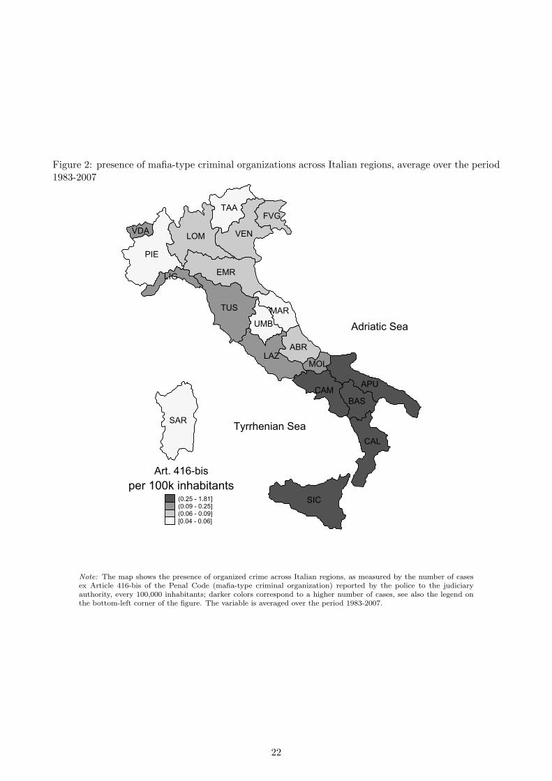
Figure 2: presence of mafia-type criminal organizations across Italian regions, average over the period1983-2007

PIE

VDALOM

TAA

VEN

FVG

LIGEMR

TUS

UMB

MAR

LAZABR

MOL

CAMAPU

BAS

CAL

SIC

SARTyrrhenian Sea

Adriatic Sea

(0.25 - 1.81](0.09 - 0.25](0.06 - 0.09]

[0.04 - 0.06]

per 100k inhabitants

Art. 416-bis

Note: The map shows the presence of organized crime across Italian regions, as measured by the number of casesex Article 416-bis of the Penal Code (mafia-type criminal organization) reported by the police to the judiciaryauthority, every 100,000 inhabitants; darker colors correspond to a higher number of cases, see also the legend onthe bottom-left corner of the figure. The variable is averaged over the period 1983-2007.

22

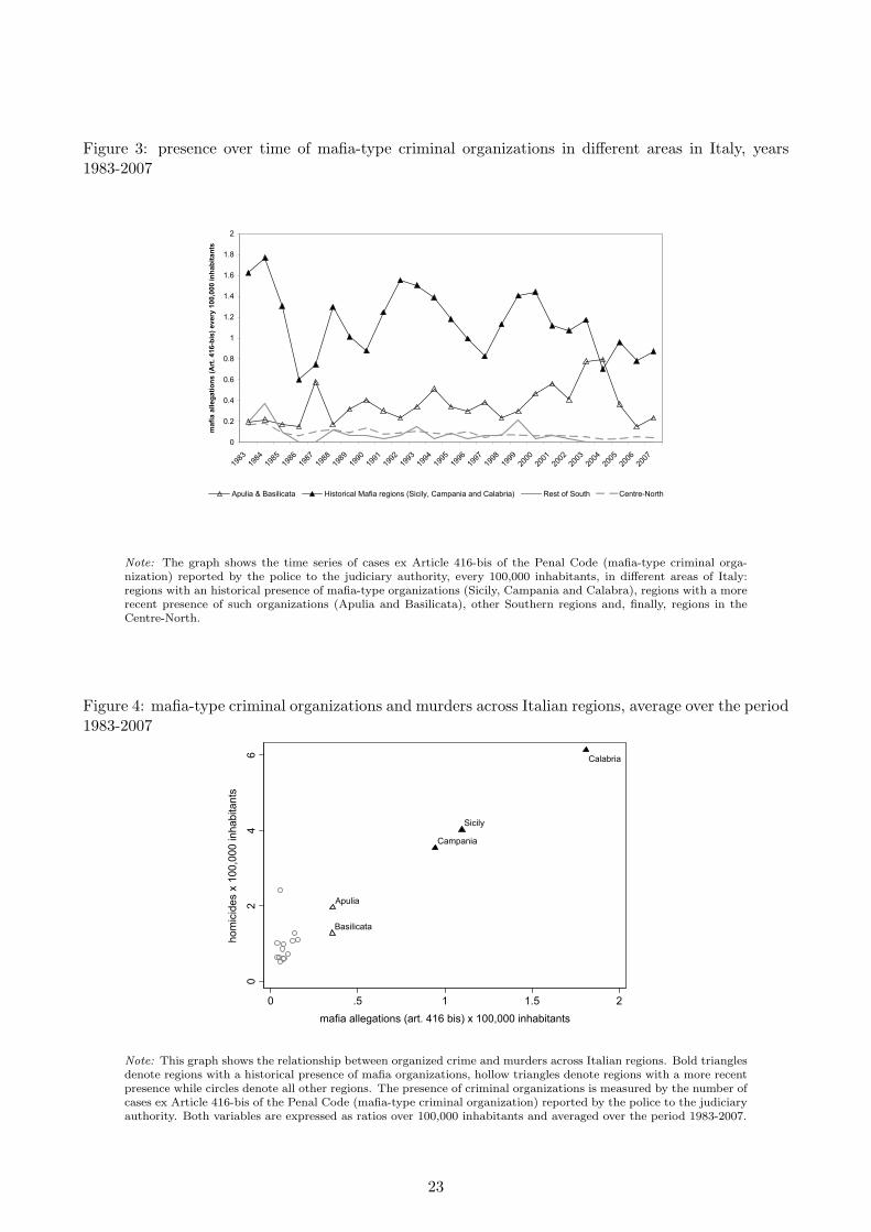
Figure 3: presence over time of mafia-type criminal organizations in different areas in Italy, years1983-2007

0

0.2

0.4

0.6

0.8

1

1.2

1.4

1.6

1.8

2

1983

1984

1985

1986

1987

1988

1989

1990

1991

1992

1993

1994

1995

1996

1997

1998

1999

2000

2001

2002

2003

2004

2005

2006

2007

mafia allegations (Art. 416-bis) every 100,000 inhabitants

Apulia & Basilicata Historical Mafia regions (Sicily, Campania and Calabria) Rest of South Centre-North

Note: The graph shows the time series of cases ex Article 416-bis of the Penal Code (mafia-type criminal orga-nization) reported by the police to the judiciary authority, every 100,000 inhabitants, in different areas of Italy:regions with an historical presence of mafia-type organizations (Sicily, Campania and Calabra), regions with a morerecent presence of such organizations (Apulia and Basilicata), other Southern regions and, finally, regions in theCentre-North.

Figure 4: mafia-type criminal organizations and murders across Italian regions, average over the period1983-2007

Campania

Calabria

Sicily

Apulia

Basilicata

02

46

hom

icid

es x

100,0

00 inhabitants

0 .5 1 1.5 2

mafia allegations (art. 416 bis) x 100,000 inhabitants

Note: This graph shows the relationship between organized crime and murders across Italian regions. Bold trianglesdenote regions with a historical presence of mafia organizations, hollow triangles denote regions with a more recentpresence while circles denote all other regions. The presence of criminal organizations is measured by the number ofcases ex Article 416-bis of the Penal Code (mafia-type criminal organization) reported by the police to the judiciaryauthority. Both variables are expressed as ratios over 100,000 inhabitants and averaged over the period 1983-2007.

23

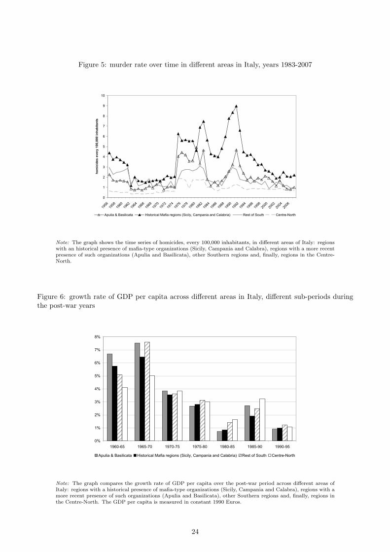
Figure 5: murder rate over time in different areas in Italy, years 1983-2007

0

1

2

3

4

5

6

7

8

9

10

1956

1958

1960

1962

1964

1966

1968

1970

1972

1974

1976

1978

1980

1982

1984

1986

1988

1990

1992

1994

1996

1998

2000

2002

2004

2006

homicides every 100,000 inhabitants

Apulia & Basilicata Historical Mafia regions (Sicily, Campania and Calabria) Rest of South Centre-North

Note: The graph shows the time series of homicides, every 100,000 inhabitants, in different areas of Italy: regionswith an historical presence of mafia-type organizations (Sicily, Campania and Calabra), regions with a more recentpresence of such organizations (Apulia and Basilicata), other Southern regions and, finally, regions in the Centre-North.

Figure 6: growth rate of GDP per capita across different areas in Italy, different sub-periods duringthe post-war years

0%

1%

2%

3%

4%

5%

6%

7%

8%

1960-65 1965-70 1970-75 1975-80 1980-85 1985-90 1990-95

Apulia & Basilicata Historical Mafia regions (Sicily, Campania and Calabria) Rest of South Centre-North

Note: The graph compares the growth rate of GDP per capita over the post-war period across different areas ofItaly: regions with a historical presence of mafia-type organizations (Sicily, Campania and Calabra), regions with amore recent presence of such organizations (Apulia and Basilicata), other Southern regions and, finally, regions inthe Centre-North. The GDP per capita is measured in constant 1990 Euros.

24

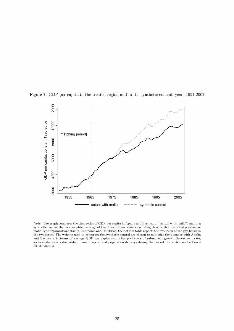
Figure 7: GDP per capita in the treated region and in the synthetic control, years 1951-2007

[matching period]

20

00

40

00

60

00

80

00

10

00

01

20

00

GD

P p

er

ca

pit

a,

co

ns

tan

t 1

99

0 e

uro

s

1955 1965 1975 1985 1995 2005

actual with mafia synthetic control

Note: The graph compares the time series of GDP per capita in Apulia and Basilicata (“actual with mafia”) and in asynthetic control that is a weighted average of the other Italian regions excluding those with a historical presence ofmafia-type organizations (Sicily, Campania and Calabria); the bottom table reports the evolution of the gap betweenthe two series. The weights used to construct the synthetic control are chosen to minimize the distance with Apuliaand Basilicata in terms of average GDP per capita and other predictors of subsequent growth (investment rate,sectoral shares of value added, human capital and population density) during the period 1951-1965; see Section 4for the details.

25

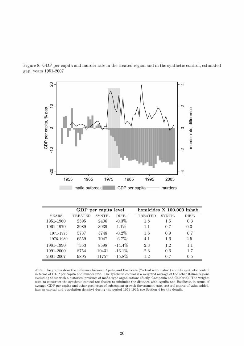
Figure 8: GDP per capita and murder rate in the treated region and in the synthetic control, estimatedgap, years 1951-2007

-4-2

02

4

murder rate, difference

-20

-10

010

20

GDP per capita, % gap

1955 1965 1975 1985 1995 2005

mafia outbreak GDP per capita murders

GDP per capita level homicides X 100,000 inhab.years treated synth. diff. treated synth. diff.

1951-1960 2395 2406 -0.3% 1.8 1.5 0.31961-1970 3989 3939 1.1% 1.1 0.7 0.3

1971-1975 5737 5748 -0.2% 1.6 0.9 0.71976-1980 6559 7047 -6.7% 4.1 1.6 2.5

1981-1990 7353 8598 -14.4% 2.3 1.2 1.11991-2000 8754 10431 -16.1% 2.3 0.6 1.72001-2007 9895 11757 -15.8% 1.2 0.7 0.5

Note: The graphs show the difference between Apulia and Basilicata (“actual with mafia”) and the synthetic controlin terms of GDP per capita and murder rate. The synthetic control is a weighted average of the other Italian regionsexcluding those with a historical presence of mafia-type organizations (Sicily, Campania and Calabria). The weightsused to construct the synthetic control are chosen to minimize the distance with Apulia and Basilicata in terms ofaverage GDP per capita and other predictors of subsequent growth (investment rate, sectoral shares of value added,human capital and population density) during the period 1951-1965; see Section 4 for the details.

26

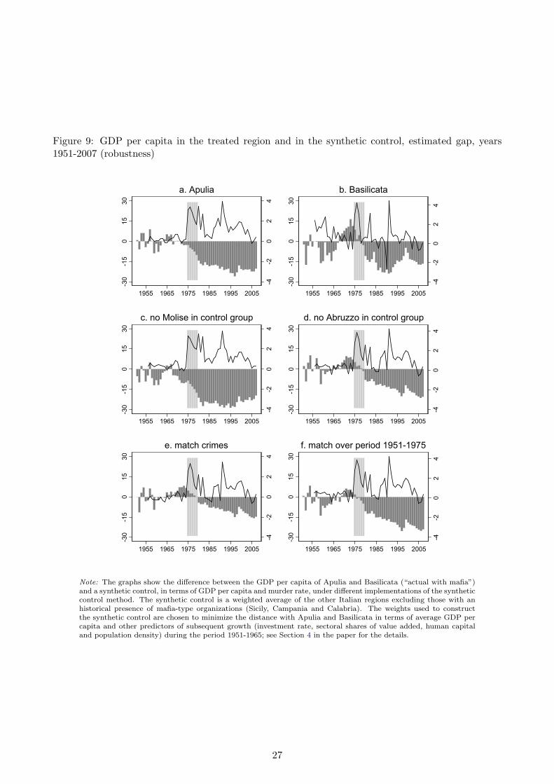
Figure 9: GDP per capita in the treated region and in the synthetic control, estimated gap, years1951-2007 (robustness)

-4-2

02

4

-30

-15

015

30

1955 1965 1975 1985 1995 2005

a. Apulia

-4-2

02

4

-30

-15

015

30

1955 1965 1975 1985 1995 2005

b. Basilicata

-4-2

02

4

-30

-15

015

30

1955 1965 1975 1985 1995 2005

c. no Molise in control group

-4-2

02

4

-30

-15

015

30

1955 1965 1975 1985 1995 2005

d. no Abruzzo in control group

-4-2

02

4

-30

-15

015

30

1955 1965 1975 1985 1995 2005

e. match crimes

-4-2

02

4

-30

-15

015

30

1955 1965 1975 1985 1995 2005

f. match over period 1951-1975

Note: The graphs show the difference between the GDP per capita of Apulia and Basilicata (“actual with mafia”)and a synthetic control, in terms of GDP per capita and murder rate, under different implementations of the syntheticcontrol method. The synthetic control is a weighted average of the other Italian regions excluding those with anhistorical presence of mafia-type organizations (Sicily, Campania and Calabria). The weights used to constructthe synthetic control are chosen to minimize the distance with Apulia and Basilicata in terms of average GDP percapita and other predictors of subsequent growth (investment rate, sectoral shares of value added, human capitaland population density) during the period 1951-1965; see Section 4 in the paper for the details.

27

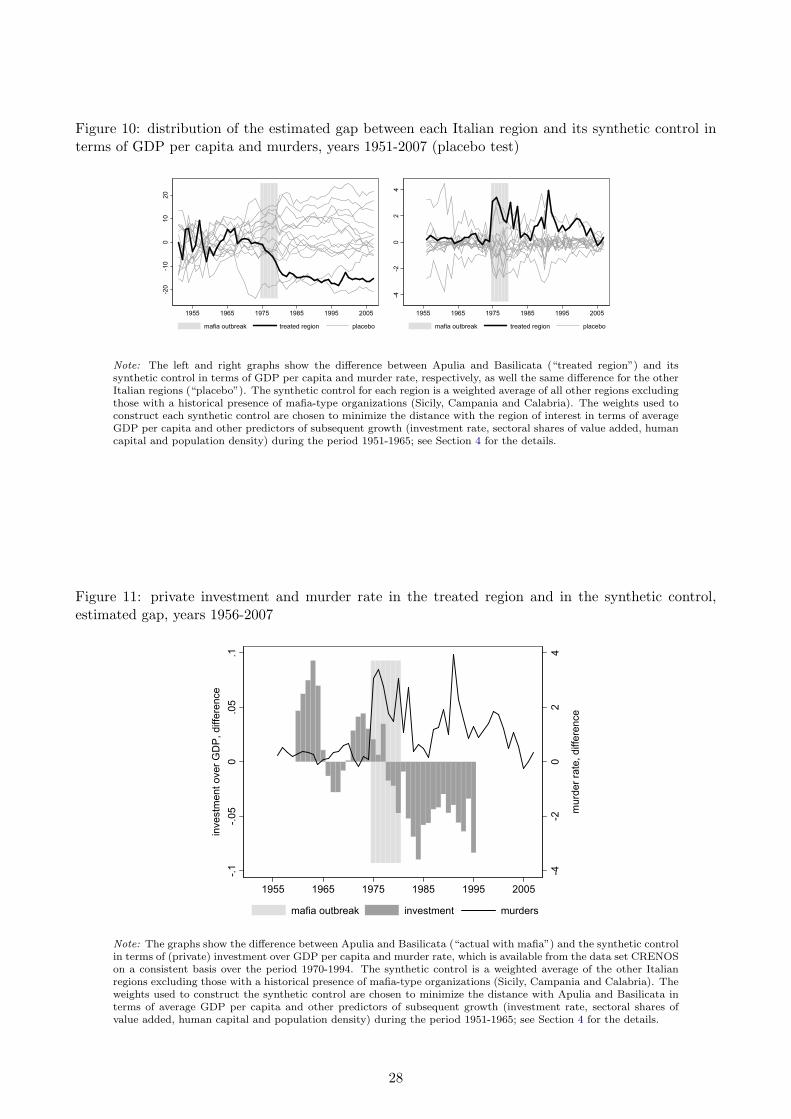
Figure 10: distribution of the estimated gap between each Italian region and its synthetic control interms of GDP per capita and murders, years 1951-2007 (placebo test)

-20

-10

010

20

1955 1965 1975 1985 1995 2005

mafia outbreak treated region placebo

-4-2

02

4

1955 1965 1975 1985 1995 2005

mafia outbreak treated region placebo

Note: The left and right graphs show the difference between Apulia and Basilicata (“treated region”) and itssynthetic control in terms of GDP per capita and murder rate, respectively, as well the same difference for the otherItalian regions (“placebo”). The synthetic control for each region is a weighted average of all other regions excludingthose with a historical presence of mafia-type organizations (Sicily, Campania and Calabria). The weights used toconstruct each synthetic control are chosen to minimize the distance with the region of interest in terms of averageGDP per capita and other predictors of subsequent growth (investment rate, sectoral shares of value added, humancapital and population density) during the period 1951-1965; see Section 4 for the details.

Figure 11: private investment and murder rate in the treated region and in the synthetic control,estimated gap, years 1956-2007

-4-2

02

4

murder rate, difference

-.1

-.05

0.05

.1

investm

ent over GDP, difference

1955 1965 1975 1985 1995 2005

mafia outbreak investment murders

Note: The graphs show the difference between Apulia and Basilicata (“actual with mafia”) and the synthetic controlin terms of (private) investment over GDP per capita and murder rate, which is available from the data set CRENOSon a consistent basis over the period 1970-1994. The synthetic control is a weighted average of the other Italianregions excluding those with a historical presence of mafia-type organizations (Sicily, Campania and Calabria). Theweights used to construct the synthetic control are chosen to minimize the distance with Apulia and Basilicata interms of average GDP per capita and other predictors of subsequent growth (investment rate, sectoral shares ofvalue added, human capital and population density) during the period 1951-1965; see Section 4 for the details.

28

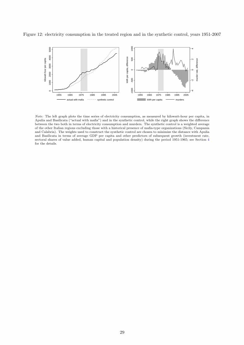
Figure 12: electricity consumption in the treated region and in the synthetic control, years 1951-2007

010

0020

0030

0040

0050

00

kilo

wat

t-ho

ur p

er c

apita

1955 1965 1975 1985 1995 2005

actual with mafia synthetic control

-4-2

02

4

mur

der

rate

, diff

eren

ce

-100

0-5

000

500

1000

kWh

per

capi

ta, d

iffer

ence

1955 1965 1975 1985 1995 2005

kWh per capita murders

Note: The left graph plots the time series of electricity consumption, as measured by kilowatt-hour per capita, inApulia and Basilicata (“actual with mafia”) and in the synthetic control, while the right graph shows the differencebetween the two both in terms of electricity consumption and murders. The synthetic control is a weighted averageof the other Italian regions excluding those with a historical presence of mafia-type organizations (Sicily, Campaniaand Calabria). The weights used to construct the synthetic control are chosen to minimize the distance with Apuliaand Basilicata in terms of average GDP per capita and other predictors of subsequent growth (investment rate,sectoral shares of value added, human capital and population density) during the period 1951-1965; see Section 4for the details.

29

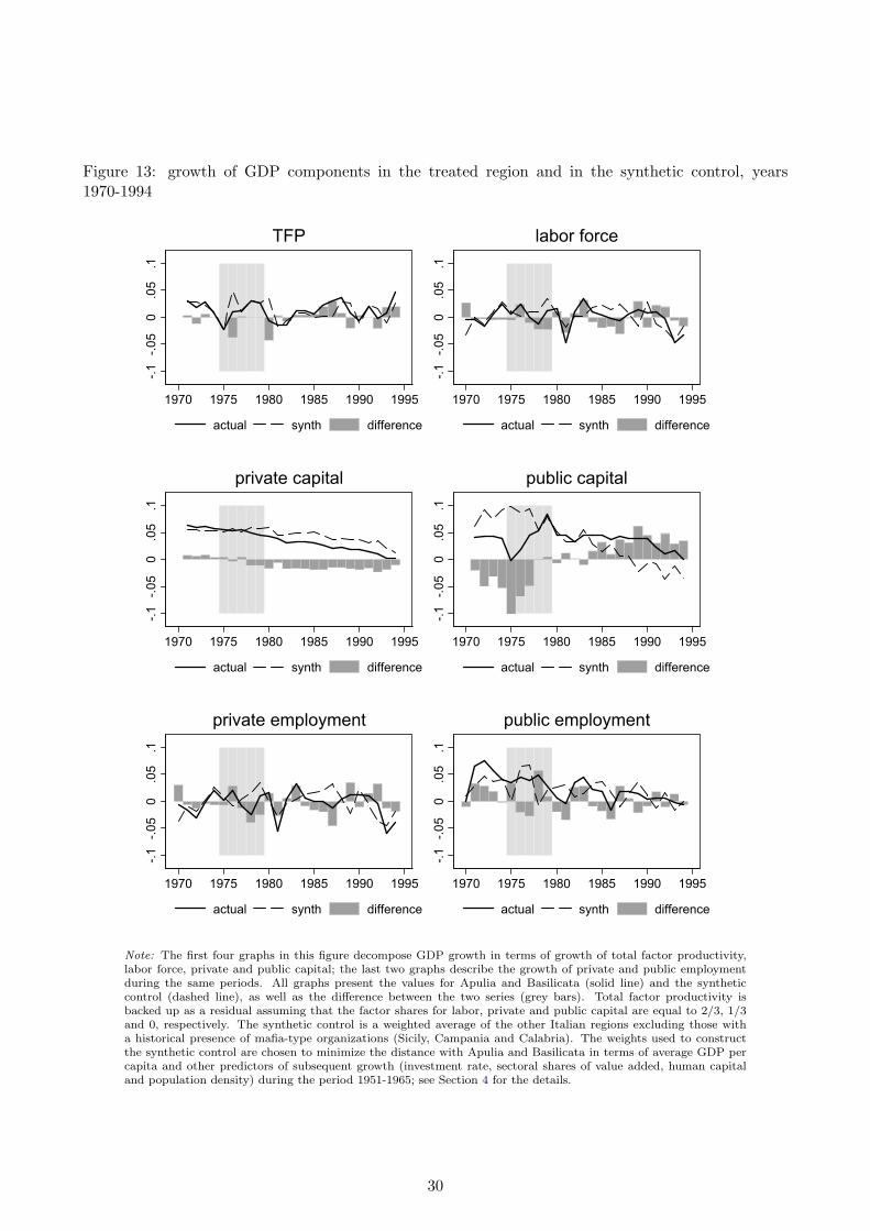
Figure 13: growth of GDP components in the treated region and in the synthetic control, years1970-1994

-.1-.05

0.05

.1

1970 1975 1980 1985 1990 1995

actual synth difference

TFP

-.1-.05

0.05

.1

1970 1975 1980 1985 1990 1995

actual synth difference

labor force

-.1-.05

0.05

.1

1970 1975 1980 1985 1990 1995

actual synth difference

private capital

-.1-.05

0.05

.1

1970 1975 1980 1985 1990 1995

actual synth difference

public capital

-.1-.05

0.05

.1

1970 1975 1980 1985 1990 1995

actual synth difference

private employment

-.1-.05

0.05

.1

1970 1975 1980 1985 1990 1995

actual synth difference

public employment

Note: The first four graphs in this figure decompose GDP growth in terms of growth of total factor productivity,labor force, private and public capital; the last two graphs describe the growth of private and public employmentduring the same periods. All graphs present the values for Apulia and Basilicata (solid line) and the syntheticcontrol (dashed line), as well as the difference between the two series (grey bars). Total factor productivity isbacked up as a residual assuming that the factor shares for labor, private and public capital are equal to 2/3, 1/3and 0, respectively. The synthetic control is a weighted average of the other Italian regions excluding those witha historical presence of mafia-type organizations (Sicily, Campania and Calabria). The weights used to constructthe synthetic control are chosen to minimize the distance with Apulia and Basilicata in terms of average GDP percapita and other predictors of subsequent growth (investment rate, sectoral shares of value added, human capitaland population density) during the period 1951-1965; see Section 4 for the details.

30

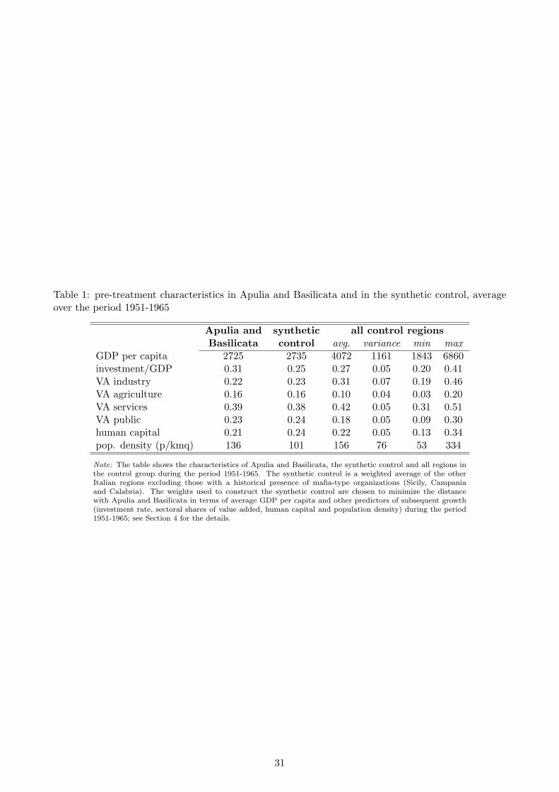
Table 1: pre-treatment characteristics in Apulia and Basilicata and in the synthetic control, averageover the period 1951-1965

Apulia and synthetic all control regionsBasilicata control avg. variance min max

GDP per capita 2725 2735 4072 1161 1843 6860investment/GDP 0.31 0.25 0.27 0.05 0.20 0.41VA industry 0.22 0.23 0.31 0.07 0.19 0.46VA agriculture 0.16 0.16 0.10 0.04 0.03 0.20VA services 0.39 0.38 0.42 0.05 0.31 0.51VA public 0.23 0.24 0.18 0.05 0.09 0.30human capital 0.21 0.24 0.22 0.05 0.13 0.34pop. density (p/kmq) 136 101 156 76 53 334

Note: The table shows the characteristics of Apulia and Basilicata, the synthetic control and all regions inthe control group during the period 1951-1965. The synthetic control is a weighted average of the otherItalian regions excluding those with a historical presence of mafia-type organizations (Sicily, Campaniaand Calabria). The weights used to construct the synthetic control are chosen to minimize the distancewith Apulia and Basilicata in terms of average GDP per capita and other predictors of subsequent growth(investment rate, sectoral shares of value added, human capital and population density) during the period1951-1965; see Section 4 for the details.

31

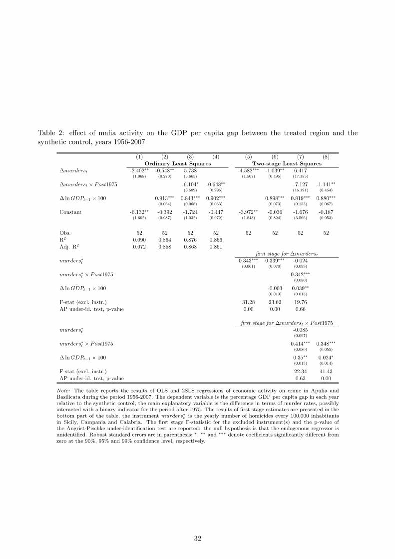
Table 2: effect of mafia activity on the GDP per capita gap between the treated region and thesynthetic control, years 1956-2007

(1) (2) (3) (4) (5) (6) (7) (8)Ordinary Least Squares Two-stage Least Squares

∆murderst -2.402∗∗ -0.548∗∗ 5.738 -4.582∗∗∗ -1.039∗∗ 6.417(1.068) (0.270) (3.665) (1.507) (0.495) (17.185)

∆murderst × Post1975 -6.104∗ -0.648∗∗ -7.127 -1.141∗∗(3.589) (0.296) (16.191) (0.454)

∆ lnGDPt−1 × 100 0.913∗∗∗ 0.843∗∗∗ 0.902∗∗∗ 0.898∗∗∗ 0.819∗∗∗ 0.880∗∗∗(0.064) (0.068) (0.063) (0.073) (0.153) (0.067)

Constant -6.132∗∗ -0.392 -1.724 -0.447 -3.972∗∗ -0.036 -1.676 -0.187(1.602) (0.987) (1.032) (0.972) (1.843) (0.824) (3.506) (0.953)

Obs. 52 52 52 52 52 52 52 52R2 0.090 0.864 0.876 0.866Adj. R2 0.072 0.858 0.868 0.861

first stage for ∆murderst

murders∗t 0.343∗∗∗ 0.339∗∗∗ -0.024(0.061) (0.070) (0.099)

murders∗t × Post1975 0.342∗∗∗(0.080)

∆ lnGDPt−1 × 100 -0.003 0.039∗∗(0.013) (0.015)

F-stat (excl. instr.) 31.28 23.62 19.76AP under-id. test, p-value 0.00 0.00 0.66

first stage for ∆murderst × Post1975murders∗t -0.085

(0.097)

murders∗t × Post1975 0.414∗∗∗ 0.348∗∗∗(0.080) (0.055)

∆ lnGDPt−1 × 100 0.35∗∗ 0.024∗(0.015) (0.014)

F-stat (excl. instr.) 22.34 41.43AP under-id. test, p-value 0.63 0.00

Note: The table reports the results of OLS and 2SLS regressions of economic activity on crime in Apulia andBasilicata during the period 1956-2007. The dependent variable is the percentage GDP per capita gap in each yearrelative to the synthetic control; the main explanatory variable is the difference in terms of murder rates, possiblyinteracted with a binary indicator for the period after 1975. The results of first stage estimates are presented in thebottom part of the table, the instrument murders∗t is the yearly number of homicides every 100,000 inhabitantsin Sicily, Campania and Calabria. The first stage F-statistic for the excluded instrument(s) and the p-value ofthe Angrist-Pischke under-identification test are reported: the null hypothesis is that the endogenous regressor isunidentified. Robust standard errors are in parenthesis; ∗, ∗∗ and ∗∗∗ denote coefficients significantly different fromzero at the 90%, 95% and 99% confidence level, respectively.

32

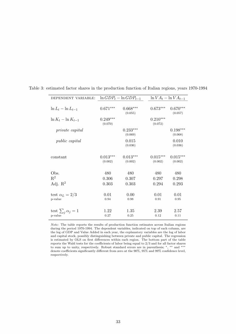
Table 3: estimated factor shares in the production function of Italian regions, years 1970-1994

dependent variable: lnGDPt − lnGDPt−1 lnV At − lnV At−1

lnLt − lnLt−1 0.671∗∗∗ 0.668∗∗∗ 0.673∗∗∗ 0.670∗∗∗(0.055) (0.057)

lnKt − lnKt−1 0.249∗∗∗ 0.210∗∗∗(0.070) (0.072)

private capital 0.233∗∗∗ 0.198∗∗∗(0.069) (0.068)

public capital 0.015 0.010(0.036) (0.036)

constant 0.013∗∗∗ 0.013∗∗∗ 0.015∗∗∗ 0.015∗∗∗(0.002) (0.002) (0.002) (0.002)

Obs. 480 480 480 480R2 0.306 0.307 0.297 0.298Adj. R2 0.303 0.303 0.294 0.293

test αL = 2/3 0.01 0.00 0.01 0.01p-value 0.94 0.98 0.91 0.95

test∑

j αj = 1 1.22 1.35 2.39 2.57p-value 0.27 0.25 0.12 0.11

Note: The table reports the results of production function estimates across Italian regionsduring the period 1970-1994. The dependent variables, indicated on top of each column, arethe log of GDP and Value Added in each year, the explanatory variables are the log of laborand capital stock, possibly distinguishing between private and public capital. The regressionis estimated by OLS on first differences within each region. The bottom part of the tablereports the Wald tests for the coefficients of labor being equal to 2/3 and for all factor sharesto sum up to unity, respectively. Robust standard errors are in parenthesis; ∗, ∗∗ and ∗∗∗

denote coefficients significantly different from zero at the 90%, 95% and 99% confidence level,respectively.

33