THE ECONOMIC AND POLICY CONSEQUENCESOF CATASTROPHES∗

by

Robert S. PindyckMassachusetts Institute of Technology

Neng WangColumbia University

This draft: March 11, 2012

Abstract: What is the likelihood that the U.S. will experience a devastating catastrophic

event over the next few decades that would substantially reduce the capital stock, GDP and

wealth? And how much should society be willing to pay to reduce the probability or impact of

a catastrophe? We show how answers to these questions can be inferred from economic data.

We provide a framework for policy analysis which is based on a general equilibrium model of

production, capital accumulation, and household preferences. Calibrating to economic and

financial data provides estimates of the annual mean arrival rate of shocks and their size

distribution, as well as investment, Tobin’s q, and the coefficient of relative risk aversion.

We use the model to calculate the tax on consumption society would accept to limit the

maximum size of a catastrophic shock, and the cost to insure against its actual impact.

JEL Classification Numbers: H56; G01, E20

Keywords: Catastrophes, disasters, rare events, economic uncertainty, market volatility,

consumption tax, catastrophe insurance, national security.

∗We thank Ben Lockwood and Jinqiang Yang for their outstanding research assistance, and Alan Auer-bach, Robert Barro, Patrick Bolton, Hui Chen, Pierre Collin-Dufresne, Chaim Fershtman, Itzhak Gilboa,Francois Gourio, Chad Jones, Dirk Krueger, Lars Lochstoer, Greg Mankiw, Jim Poterba, Julio Rotemberg,Suresh Sundaresan, two anonymous referees, and seminar participants at Columbia, Hebrew University ofJerusalem, M.I.T., the NBER, and Tel-Aviv University for helpful comments and suggestions.

1 Introduction.

What is the likelihood that the U.S. will experience a devastating catastrophic event over

the next few decades? And how much should society be willing to pay to limit the possible

impact of such an event? By “catastrophic event,” we mean something national or global

in scale that would substantially reduce the capital stock and/or the productive efficiency

of capital, thereby substantially reducing GDP, consumption, and wealth. Examples might

include a nuclear or biological terrorist attack (far worse than even 9/11), a highly contagious

“mega-virus” that spreads uncontrollably, a global environmental disaster, or a financial and

economic crisis on the order of the Great Depression.1 We show how the probability and

possible impact of such an event can be inferred from the behavior of economic and financial

variables such as investment, interest rates, and equity returns. We also show how our

framework can be used to estimate the amount society should be willing to pay to reduce

the probability of a catastrophic event, or to insure against its actual impact should it occur.

An emerging literature has used historical data to estimate the likelihood and expected

impact of catastrophic events.2 Examples include Barro (2006, 2009), Barro and Ursua

(2008), and Barro, Nakamura, Steinsson, and Ursua (2009).3 These studies, however, are

limited in two respects. First, many of the included disasters are manifestations of three

global events — the two World Wars and the Great Depression. Second, the possible catas-

trophic events that we think are of greatest interest today have little or no historical precedent

1Readers who are incurable optimists or have limited imaginations should read Posner (2004), who pro-vides more examples and argues that society fails to take these risks seriously enough, and Sunstein (2007).For a sobering discussion of the likelihood and possible impact of nuclear terrorism, see Allison (2004).

2The roots of this literature go back to the observation by Rietz (1988) that low-probability catastrophesmight explain the equity premium puzzle first noted by Mehra and Prescott (1985), i.e., could help reconcilea relatively large equity premium (5 to 7%) and low real risk-free rate of interest (0 to 2%) with moderaterisk aversion on the part of households. Weitzman (2007) has shown that the equity premium and realrisk-free rate puzzles could alternatively be explained by “structural uncertainty” in which one or more keyparameters, such as the true variance of equity returns, is estimated through Bayesian updating.

3In related work, Gourio (2008) modeled an exchange economy with recursive preferences and disastersthat have limited duration. He found that the effect of recoveries on the equity premium could be positiveor negative, depending on the elasticity of intertemporal substitution. Gabaix (2008) and Wachter (2008)showed that a time-varying disaster arrival rate could explain the high volatility of the stock market (inaddition to the equity premium and real risk-free rate).

1

— there are no data, for example, on the frequency or impact of nuclear or biological terror-

ist attacks. Or consider the forty-year period beginning around 1950 and ending with the

breakup of the Soviet Union, during which one potential catastrophic event dominated all

others: the possibility of a U.S.-Soviet nuclear war. The Department of Defense, the RAND

Corporation and others studied the likelihood and potential impact of such an event, but

there was no historical precedent on which to base estimates.

We take a different approach from earlier studies and ask what event arrival rate and

impact distribution are implied by the behavior of basic economic and financial variables.

We do not try to estimate the characteristics of catastrophic events from historical data

on drops in consumption or GDP, nor do we use the estimates of others. Instead, we

develop an equilibrium model of the economy that incorporates catastrophic shocks to the

capital stock, and that links the first four moments of equity returns, along with economic

variables such as consumption, investment, interest rates, and Tobin’s q, to parameters

describing the characteristics of shocks as well as behavioral parameters such as the coefficient

of relative risk aversion and elasticity of intertemporal substitution. We can then determine

the characteristics of catastrophes as a calibration output of our analysis. In effect, we are

assuming that these characteristics are those perceived by firms and households, in that they

are consistent with the data for key economic and financial variables.4

Our framework also provides a tool for policy analysis. For example, how much should

society be willing to pay to reduce or limit the impact of a catastrophic event? To measure

“willingness to pay” (WTP), we calculate the maximum permanent percentage tax rate that

society should be willing to accept in order to eliminate the possibility of a catastrophic

shock, or reduce the maximum possible impact of such as shock. We also show how our

framework can be used to calculate the equilibrium price of insurance against catastrophic

risk, and we compare the use of insurance to the cost of reducing or eliminating risk.

In the next section we lay out a parsimonious model with an AK production technology,

4In related work, Russett and Slemrod (1993) used survey data to show how beliefs about the likelihoodof nuclear war affected savings behavior, and argue that such beliefs can help explain the low propensity tosave in the U.S. relative to other countries. Also, see Slemrod (1990) and Russett and Lackey (1987).

2

adjustment costs (which we show are crucial), and shocks that arrive unpredictably. Each

shock destroys a random fraction of the capital stock. We treat as catastrophic those shocks

that reduce the capital stock by a “large” amount, e.g., something more than 10 or 15 percent.

We explain how the model’s calibration yields information about the characteristics of shocks,

as well as important behavioral parameters, and we show how all of the parameters of the

model can be identified on a block-wise basis. Proceeding in stages, we show (1) how the

variance, skewness, and kurtosis of equity returns identifies the parameters that characterize

both unpredictable shocks and continuous fluctuations in the capital stock; (2) how the

equity risk premium can then be used to identify the coefficient of relative risk aversion;

(3) how, given these parameters, the risk-free interest rate then identifies the elasticity of

intertemporal substitution and/or the rate of time preference; and (4) how the consumption-

investment ratio and the real growth rate of GDP then determine the marginal propensity

to consume, Tobin’s q, and investment. We also explain how the calibrated model can be

used to determine the equilibrium price of insurance against catastrophic risk.

To calibrate the model, we use data for the U.S. economy and financial markets over

the period 1947 through 2008. Section 3 presents our calibration results and discusses their

implications for the characteristics of shocks and for behavioral parameters. Section 3 also

shows the implications of the model for the price of insurance against catastrophes of var-

ious sizes, and demonstrates the importance of adjustment costs. Section 4 discusses the

application of our framework to policy analysis. In particular, we calculate the maximum

permanent tax on consumption that society would accept to reduce or eliminate the impact

of catastrophic shocks. Section 5 concludes.

2 Framework.

In this section we lay out the building blocks of a simple general equilibrium model, and

then explain how the model is solved.

3

2.1 Building Blocks.

Preferences. We use the Duffie and Epstein (1992) continuous-time version of Epstein-

Weil-Zin (EWZ) preferences, so that a representative consumer has homothetic recursive

preferences given by:5

Vt = Et[∫ ∞t

f(Cs, Vs)ds], (1)

where

f(C, V ) =ρ

1− ψ−1

C1−ψ−1 − ((1− γ)V )ω

((1− γ)V )ω−1 . (2)

Here ρ is the rate of time preference, ψ the elasticity of intertemporal substitution (EIS),

γ the coefficient of relative risk aversion, and we define ω = (1 − ψ−1)/(1 − γ). Unlike

time-additive utility, recursive preferences as defined by eqns. (1) and (2) disentangle risk

aversion from the EIS. Note that with these preferences, the marginal benefit of consumption

is fC = ρC−ψ−1/[(1 − γ)V ]ω−1, which depends not only on current consumption but also

(through V ) on the expected trajectory of future consumption.

If γ = ψ−1 so that ω = 1, we have the standard constant-relative-risk-aversion (CRRA)

expected utility, represented by the additively separable aggregator:

f(C, V ) =ρC1−γ

1− γ− ρV. (3)

One of the questions we address is whether γ is close to ψ−1, so that the simple CRRA utility

function is a reasonable approximation for modeling purposes. More generally, we examine

how equilibrium allocation and pricing constrains the model’s parameters, including the EIS

and the coefficient of relative risk aversion.

Production. Aggregate output has an AK production technology:

Y = AK , (4)

where A is a constant that defines productivity and the capital stock K is the sole factor of

production. The AK model is widely used, in part because it generates balanced growth in

5Epstein and Zin (1989) and Weil (1990) developed homothetic non-expected utility in discrete time,which separates the elasticity of intertermporal substitution from the coefficient of relative risk aversion.

4

equilibrium. In our specification, K is the total stock of capital; it includes physical capital

as traditionally measured, but also human capital and firm-based intangible capital (such

as, patents, know-how, brand value, and organizational capital).

Shocks to the Capital Stock. We assume that discrete downward jumps to the capital

stock (“shocks”) occur as Poisson arrivals with a mean arrival rate λ. There is no limit to the

number of these shocks; the occurrence of a shock does not change the likelihood of another,

and in principle shocks can occur frequently.6 When a shock does occur, it permanently

destroys a stochastic fraction (1 − Z) of the capital stock K, so that Z is the remaining

fraction. (For example, if a particular shock destroyed 15 percent of capital stock, we would

have Z = .85.) We assume that Z follows a well-behaved probability density function (pdf)

ζ(Z) with 0 ≤ Z ≤ 1. By well-behaved, we mean that the moments E(Zn) exist for n = 1,

1 − γ, and −γ. As we will see, these are the only moments of Z that are relevant for our

analysis.

As we will show in Section 3 when we discuss the calibration of the model, shocks occur

frequently, but for most shocks losses are small. We consider catastrophes to be shocks for

which the drop in the capital stock is sufficiently large, e.g., more than 10 or 15 percent.

Using our calibration, we will see that the model predicts that catastrophic shocks are rare.

The capital stock is also subject to ongoing continuous fluctuations. These continuous

fluctuations, along with small jumps, can be thought of as the stochastic depreciation of

capital. Large shocks, on the other hand, are interpreted as (rare) catastrophic events.

Investment and Capital Accumulation. Letting I denote aggregate investment, the

capital stock K evolves as:

dKt = Φ(It, Kt)dt+ σKtdWt − (1− Z)KtdJt . (5)

Here the parameter σ captures diffusion volatility, Wt is a standard Brownian motion process,

and Jt is a jump process with mean arrival rate λ that captures discrete shocks; if a jump

6Stochastic fluctuations in the capital stock have been widely used in the growth literature with an AKtechnology, but unlike the existing literature, we examine the economic effects of shocks to capital thatinvolve discrete (catastrophic) jumps. See Jones and Manuelli (2005) for a survey of endogenous growthmodels with with a stochastic AK technology.

5

occurs, K falls by the random fraction (1 − Z). The adjustment cost function Φ(I,K)

captures effects of depreciation and costs of installing capital. Because installing capital

is costly, installed capital earns rents in equilibrium so that Tobin’s q, the ratio between

the market value and the replacement cost of capital, exceeds one. We assume Φ(I,K) is

homogeneous of degree one in I and K and thus can be written as:

Φ(I,K) = φ(i)K , (6)

where i = I/K and φ(i) is increasing and concave. Unlike other models of catastrophes, we

explicitly account for the effects of adjustment costs on equilibrium price and quantities.7

For simplicity, we use a quadratic adjustment cost function, which can be viewed as a

second-order approximation to a more general one:

φ(i) = i− 12θi2 − δ . (7)

Catastrophic Risk Insurance. We will use our model allows us to determine the equi-

librium premium for catastrophic risk insurance. In order to make our analysis of insurance

as general as possible, we introduce catastrophic insurance swaps (CIS) for shocks of every

possible size as follows. These swaps are defined as follows: a CIS for the survival fraction

in the interval (Z,Z + dZ) is a swap contract in which the buyer makes a continuum of pay-

ments p(Z)dZ to the seller and in exchange receives a lump-sum payoff if and only if a shock

with survival fraction in (Z,Z+dZ) occurs. That is, the buyer stops paying the seller if and

only if the defined catastrophic event occurs and then collects one unit of the consumption

good as a payoff from the seller. Note the close analogy between our CIS contracts and the

widely used credit default swap (CDS) contracts. Unlike typical pricing models for CDS

contracts, however, ours is a general equilibrium model with an endogenously determined

risk premium.

7Homogeneous adjustment cost functions are analytically tractable and have been widely used in the qtheory of investment literature. Hayashi (1982) showed that with homogeneous adjustment costs and perfectcapital markets, marginal and average q are equal. Jermann (1998) integrated this type of adjustment costsinto an equilibrium business cycle/asset pricing model.

6

2.2 Competitive Equilibrium.

Our model can be solved as a social planning problem, but we want to assert that the result

is equivalent to a decentralized competitive equilibrium with complete markets. That is, we

assume that the following securities can be traded at each point in time: (i) a risk-free asset,

(ii) a claim on the value of capital of the representative firm, and (iii) insurance claims for

catastrophes with every possible recovery fraction Z.

Because we allow for jumps in the capital stock, market completeness requires that agents

can trade these insurance claims. But note that as with the risk-free asset, in equilibrium

the demand for these insurance claims is zero. Although no trading of the risk-free asset

or insurance claims will occur in equilibrium, we allow for the possibility of trading so that

we can determine the equilibrium prices. In a representative agent model like ours, this

“zero demand” result is a natural consequence. With heterogeneous agents (differing, e.g.,

in preferences, endowments, or beliefs), there will be no trading in general. but some agents

will be buyers and some sellers of these assets. However, the net demand for the risk-free

and insurance assets will be zero (as implied by market clearing.

We define the recursive competitive equilibrium as follows: (1) The representative con-

sumer dynamically chooses investments in the risk-free asset, risky equity, and various CIS

claims to maximize utility as given by eqns. (1) and (2). These choices are made taking

the equilibrium prices of all assets and investment/consumption goods as given. (2) The

representative firm chooses the level of investment that maximizes its market value, which is

the present discounted value of future cash flows, using the equilibrium stochastic discount

factor. (3) All markets clear. In particular, (i) the net supply of the risk-free asset is zero;

(ii) the demand for the claim to the representative firm is equal to unity, the normalized

aggregate supply; (iii) the net demand for the CIS of each possible recovery fraction Z is

zero; and (iv) the goods market clears, i.e., It = Yt − Ct at all t ≥ 0.

These market-clearing conditions are standard. When all markets are available for trading

by investors and firms, the prices of claims such as the risk-free asset and CIS claims are

at levels implying zero demand in equilibrium. With these conditions, we can invoke the

7

welfare theorem to solve the social planner’s problem and obtain the competitive equilibrium

allocation, and then use the representative agent’s marginal utility to price all assets in the

economy. We emphasize that CIS insurance markets are crucial to dynamically complete the

markets. This is a fundamental difference from models based purely on diffusion processes

without jump risk.

We next summarize the solution of the model via the social planner’s problem, leaving

details to Appendix A. A separate appendix, available from the authors on request, derives

the decentralized competitive market equilibrium and shows that it yields the same solution.

2.3 Model Solution.

The Hamilton-Jacobi-Bellman (HJB) equation for the social planner’s allocation problem is:

0 = maxC

{f(C, V ) + Φ(I,K)V ′(K) +

1

2σ2K2V ′′(K) + λE [V (ZK)− V (K)]

}, (8)

where V (K) is the value function and the expectation is with respect to the density function

ζ(Z) for the survival fraction Z. We have the following first-order condition for I:

fC(C, V ) = ΦI(I,K)V ′(K) . (9)

The left-hand side of eqn. (9) is the marginal benefit of consumption and the right-hand side

is its marginal cost, which equals the marginal value of capital V ′(K) times the marginal

efficiency of converting a unit of the consumption good into a unit of capital, ΦI(I,K). With

homogeneity, we have ΦI(I,K) = φ′(i).

We will show that the value function is homogeneous and takes the following form:

V (K) =1

1− γ(bK)1−γ , (10)

where b is a coefficient determined as part of the solution. Let c = C/K = A−i. (Lower-case

letters in this paper express quantities relative to the capital stock K.) Appendix A shows

that b is related to the equilibrium level of the investment-capital ratio, i∗, by:

b = (A− i∗)1/(1−ψ)

(ρ

φ′(i∗)

)−ψ/(1−ψ)

. (11)

8

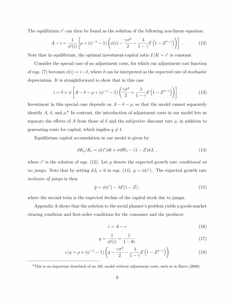
The equilibrium i∗ can then be found as the solution of the following non-linear equation:

A− i =1

φ′(i)

[ρ+ (ψ−1 − 1)

(φ(i)− γσ2

2− λ

1− γE(1− Z1−γ

))]. (12)

Note that in equilibrium, the optimal investment-capital ratio I/K = i∗ is constant.

Consider the special case of no adjustment costs, for which our adjustment cost function

of eqn. (7) becomes φ(i) = i−δ, where δ can be interpreted as the expected rate of stochastic

depreciation. It is straightforward to show that in this case

i = δ + ψ

[A− δ − ρ+ (ψ−1 − 1)

(γσ2

2+

λ

1− γE(1− Z1−γ

))]. (13)

Investment in this special case depends on A − δ − ρ, so that the model cannot separately

identify A, δ, and ρ.8 In contrast, the introduction of adjustment costs in our model lets us

separate the effects of A from those of δ and the subjective discount rate ρ, in addition to

generating rents for capital, which implies q 6= 1.

Equilibrium capital accumulation in our model is given by:

dKt/Kt = φ(i∗)dt+ σdWt − (1− Z)dJt , (14)

where i∗ is the solution of eqn. (12). Let g denote the expected growth rate conditional on

no jumps. Note that by setting dJt = 0 in eqn. (14), g = φ(i∗) . The expected growth rate

inclusive of jumps is then

g = φ(i∗)− λE(1− Z) , (15)

where the second term is the expected decline of the capital stock due to jumps.

Appendix A shows that the solution to the social planner’s problem yields a goods-market

clearing condition and first-order conditions for the consumer and the producer:

i = A− c (16)

q =1

φ′(i)=

1

1− θi(17)

c/q = ρ+ (ψ−1 − 1)

(g − γσ2

2− λ

1− γE(1− Z1−γ

))(18)

8This is an important drawback of an AK model without adjustment costs, such as in Barro (2009).

9

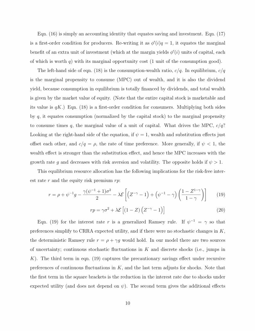
Eqn. (16) is simply an accounting identity that equates saving and investment. Eqn. (17)

is a first-order condition for producers. Re-writing it as φ′(i)q = 1, it equates the marginal

benefit of an extra unit of investment (which at the margin yields φ′(i) units of capital, each

of which is worth q) with its marginal opportunity cost (1 unit of the consumption good).

The left-hand side of eqn. (18) is the consumption-wealth ratio, c/q. In equilibrium, c/q

is the marginal propensity to consume (MPC) out of wealth, and it is also the dividend

yield, because consumption in equilibrium is totally financed by dividends, and total wealth

is given by the market value of equity. (Note that the entire capital stock is marketable and

its value is qK.) Eqn. (18) is a first-order condition for consumers. Multiplying both sides

by q, it equates consumption (normalized by the capital stock) to the marginal propensity

to consume times q, the marginal value of a unit of capital. What drives the MPC, c/q?

Looking at the right-hand side of the equation, if ψ = 1, wealth and substitution effects just

offset each other, and c/q = ρ, the rate of time preference. More generally, if ψ < 1, the

wealth effect is stronger than the substitution effect, and hence the MPC increases with the

growth rate g and decreases with risk aversion and volatility. The opposite holds if ψ > 1.

This equilibrium resource allocation has the following implications for the risk-free inter-

est rate r and the equity risk premium rp:

r = ρ+ ψ−1g − γ(ψ−1 + 1)σ2

2− λE

[(Z−γ − 1

)+(ψ−1 − γ

)(1− Z1−γ

1− γ

)](19)

rp = γσ2 + λE[(1− Z)

(Z−γ − 1

)](20)

Eqn. (19) for the interest rate r is a generalized Ramsey rule. If ψ−1 = γ so that

preferences simplify to CRRA expected utility, and if there were no stochastic changes in K,

the deterministic Ramsey rule r = ρ + γg would hold. In our model there are two sources

of uncertainty; continuous stochastic fluctuations in K and discrete shocks (i.e., jumps in

K). The third term in eqn. (19) captures the precautionary savings effect under recursive

preferences of continuous fluctuations in K, and the last term adjusts for shocks. Note that

the first term in the square brackets is the reduction in the interest rate due to shocks under

expected utility (and does not depend on ψ). The second term gives the additional effects

10

of shock risk for non-expected utility; when ψ−1 < γ, the risk of shocks further increases the

equilibrium interest rate from the level implied by standard CRRA utility.

Eqn. (20) describes the equity risk premium, rp. The first term on the RHS is the usual

risk premium in diffusion models, and the second term is the increase in the premium due

to jumps in K. When a jump occurs, (1 − Z) is the fraction of loss, and (Z−γ − 1) is

the percentage increase in marginal utility from that loss, i.e., the price of risk. The jump

component of the equity risk premium is given by λ times the expectation of the product

of these two random variables. Note that the fraction of loss and the increase of marginal

utility are positively correlated, which substantially contributes to the risk premium. (In

the limiting case where the loss is close to 100%, the increase in marginal utility approaches

infinity.) Also note that the risk premium depends only on the coefficient of risk aversion,

and does not depend on the EIS or rate of time preference.

The model can also be used to determine the equilibrium price of catastrophic risk in-

surance. We will examine the price of insurance in the next section when we discuss the

calibration of the model, after specifying the distribution ζ(Z) for Z.

3 Calibration.

This section explains our calibration procedure. We begin by specifying the probability

distribution for the survival fraction Z, and we show how this distribution simplifies the

model and also yields identifying conditions on the second, third, and fourth moments of

equity returns. Those conditions along with the other equations of the model can be used to

identify the various parameters. We describe the data used to obtain values for the model’s

inputs, and we present a baseline calibration and additional sensitivity calibrations. We turn

next to the pricing of catastrophic risk insurance, and show insurance premia for different

size losses. Lastly, we turn to the role of adjustment costs and compare our results with those

of Barro (2009). This helps to show the importance of adjustment costs and the implications

of certain parameter choices.

11

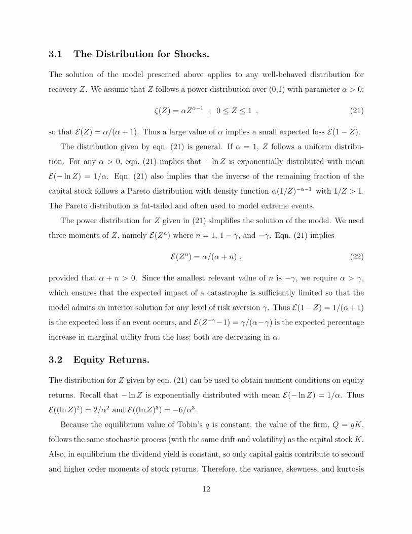
3.1 The Distribution for Shocks.

The solution of the model presented above applies to any well-behaved distribution for

recovery Z. We assume that Z follows a power distribution over (0,1) with parameter α > 0:

ζ(Z) = αZα−1 ; 0 ≤ Z ≤ 1 , (21)

so that E(Z) = α/(α + 1). Thus a large value of α implies a small expected loss E(1− Z).

The distribution given by eqn. (21) is general. If α = 1, Z follows a uniform distribu-

tion. For any α > 0, eqn. (21) implies that − lnZ is exponentially distributed with mean

E(− lnZ) = 1/α. Eqn. (21) also implies that the inverse of the remaining fraction of the

capital stock follows a Pareto distribution with density function α(1/Z)−α−1 with 1/Z > 1.

The Pareto distribution is fat-tailed and often used to model extreme events.

The power distribution for Z given in (21) simplifies the solution of the model. We need

three moments of Z, namely E(Zn) where n = 1, 1− γ, and −γ. Eqn. (21) implies

E(Zn) = α/(α + n) , (22)

provided that α + n > 0. Since the smallest relevant value of n is −γ, we require α > γ,

which ensures that the expected impact of a catastrophe is sufficiently limited so that the

model admits an interior solution for any level of risk aversion γ. Thus E(1−Z) = 1/(α+ 1)

is the expected loss if an event occurs, and E(Z−γ−1) = γ/(α−γ) is the expected percentage

increase in marginal utility from the loss; both are decreasing in α.

3.2 Equity Returns.

The distribution for Z given by eqn. (21) can be used to obtain moment conditions on equity

returns. Recall that − lnZ is exponentially distributed with mean E(− lnZ) = 1/α. Thus

E((lnZ)2) = 2/α2 and E((lnZ)3) = −6/α3.

Because the equilibrium value of Tobin’s q is constant, the value of the firm, Q = qK,

follows the same stochastic process (with the same drift and volatility) as the capital stock K.

Also, in equilibrium the dividend yield is constant, so only capital gains contribute to second

and higher order moments of stock returns. Therefore, the variance, skewness, and kurtosis

12

for logarithmic equity returns over the time interval (t, t + ∆t) equal the corresponding

moments for lnKt+∆t/Kt. Let V ,S, and K denote the variance, skewness, and kurtosis,

respectively, for equity returns. We show in Appendix B that they are given by:

V = ∆t(σ2 + 2λ/α2

)(23)

S =1√∆t

−6λ/α3

(σ2 + 2λ/α2)3/2(24)

K = 3 +1

∆t

24λ/α4

(σ2 + 2λ/α2)2(25)

Here ∆t is the frequency with which returns are measured. In our case returns are measured

monthly and are in monthly terms; because all variables are expressed in annual terms for

purposes of our calibration, ∆t = 1/12.

Using eqn. (22), the expected growth rate that includes possible jumps is

g = g − λ

α + 1. (26)

Eqn. (22) can also be used to simplify eqns. (18), (19), and (20), which now become:

c

q= r + rp− g (27)

r = ρ+ ψ−1g − γ(ψ−1 + 1)σ2

2− λ

[(ψ−1 − γ)(α− γ) + γ(α− γ + 1)

(α− γ)(α− γ + 1)

](28)

rp = γσ2 + λγ

[1

α− γ− α

(α + 1)(α + 1− γ)

](29)

Recall that in equilibrium the consumption-wealth ratio c/q is equal to the dividend yield.

Eqn. (27) is essentially a Gordon growth formula; it states that the expected return on equity

(r+ rp) equals the dividend yield (c/q) plus the expected growth rate g (inclusive of jumps).

3.3 Identification.

With eqns. (16), (17), and (23) to (29) we can identify the key parameters and variables

of the model. To do this we use the following inputs: the variance, skewness, and kurtosis

of equity returns, the real risk-free rate r and equity premium rp, the output/capital ratio

Y/K, the consumption/investment ratio c/i, and the per capita expected real growth rate g.

13

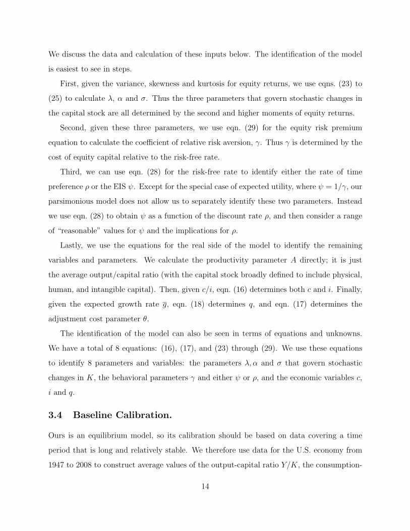
We discuss the data and calculation of these inputs below. The identification of the model

is easiest to see in steps.

First, given the variance, skewness and kurtosis for equity returns, we use eqns. (23) to

(25) to calculate λ, α and σ. Thus the three parameters that govern stochastic changes in

the capital stock are all determined by the second and higher moments of equity returns.

Second, given these three parameters, we use eqn. (29) for the equity risk premium

equation to calculate the coefficient of relative risk aversion, γ. Thus γ is determined by the

cost of equity capital relative to the risk-free rate.

Third, we can use eqn. (28) for the risk-free rate to identify either the rate of time

preference ρ or the EIS ψ. Except for the special case of expected utility, where ψ = 1/γ, our

parsimonious model does not allow us to separately identify these two parameters. Instead

we use eqn. (28) to obtain ψ as a function of the discount rate ρ, and then consider a range

of “reasonable” values for ψ and the implications for ρ.

Lastly, we use the equations for the real side of the model to identify the remaining

variables and parameters. We calculate the productivity parameter A directly; it is just

the average output/capital ratio (with the capital stock broadly defined to include physical,

human, and intangible capital). Then, given c/i, eqn. (16) determines both c and i. Finally,

given the expected growth rate g, eqn. (18) determines q, and eqn. (17) determines the

adjustment cost parameter θ.

The identification of the model can also be seen in terms of equations and unknowns.

We have a total of 8 equations: (16), (17), and (23) through (29). We use these equations

to identify 8 parameters and variables: the parameters λ, α and σ that govern stochastic

changes in K, the behavioral parameters γ and either ψ or ρ, and the economic variables c,

i and q.

3.4 Baseline Calibration.

Ours is an equilibrium model, so its calibration should be based on data covering a time

period that is long and relatively stable. We therefore use data for the U.S. economy from

1947 to 2008 to construct average values of the output-capital ratio Y/K, the consumption-

14

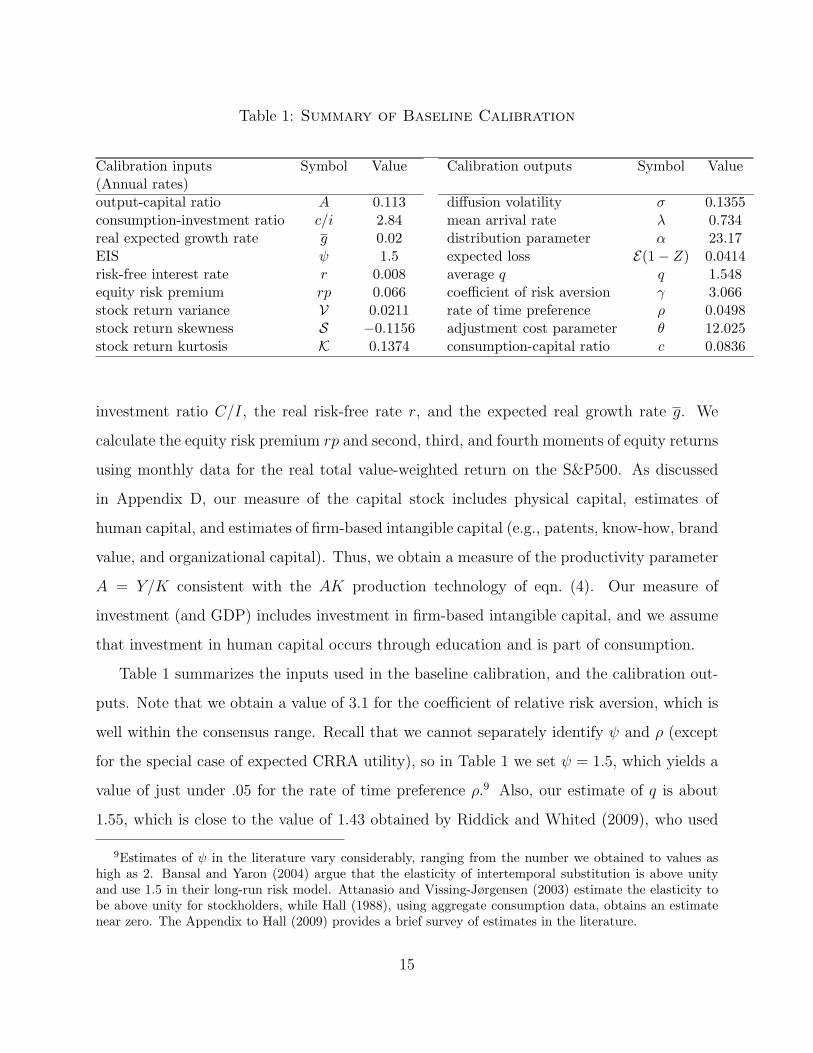
Table 1: Summary of Baseline Calibration

Calibration inputs Symbol Value Calibration outputs Symbol Value(Annual rates)output-capital ratio A 0.113 diffusion volatility σ 0.1355consumption-investment ratio c/i 2.84 mean arrival rate λ 0.734real expected growth rate g 0.02 distribution parameter α 23.17EIS ψ 1.5 expected loss E(1− Z) 0.0414risk-free interest rate r 0.008 average q q 1.548equity risk premium rp 0.066 coefficient of risk aversion γ 3.066stock return variance V 0.0211 rate of time preference ρ 0.0498stock return skewness S −0.1156 adjustment cost parameter θ 12.025stock return kurtosis K 0.1374 consumption-capital ratio c 0.0836

investment ratio C/I, the real risk-free rate r, and the expected real growth rate g. We

calculate the equity risk premium rp and second, third, and fourth moments of equity returns

using monthly data for the real total value-weighted return on the S&P500. As discussed

in Appendix D, our measure of the capital stock includes physical capital, estimates of

human capital, and estimates of firm-based intangible capital (e.g., patents, know-how, brand

value, and organizational capital). Thus, we obtain a measure of the productivity parameter

A = Y/K consistent with the AK production technology of eqn. (4). Our measure of

investment (and GDP) includes investment in firm-based intangible capital, and we assume

that investment in human capital occurs through education and is part of consumption.

Table 1 summarizes the inputs used in the baseline calibration, and the calibration out-

puts. Note that we obtain a value of 3.1 for the coefficient of relative risk aversion, which is

well within the consensus range. Recall that we cannot separately identify ψ and ρ (except

for the special case of expected CRRA utility), so in Table 1 we set ψ = 1.5, which yields a

value of just under .05 for the rate of time preference ρ.9 Also, our estimate of q is about

1.55, which is close to the value of 1.43 obtained by Riddick and Whited (2009), who used

9Estimates of ψ in the literature vary considerably, ranging from the number we obtained to values ashigh as 2. Bansal and Yaron (2004) argue that the elasticity of intertemporal substitution is above unityand use 1.5 in their long-run risk model. Attanasio and Vissing-Jørgensen (2003) estimate the elasticity tobe above unity for stockholders, while Hall (1988), using aggregate consumption data, obtains an estimatenear zero. The Appendix to Hall (2009) provides a brief survey of estimates in the literature.

15

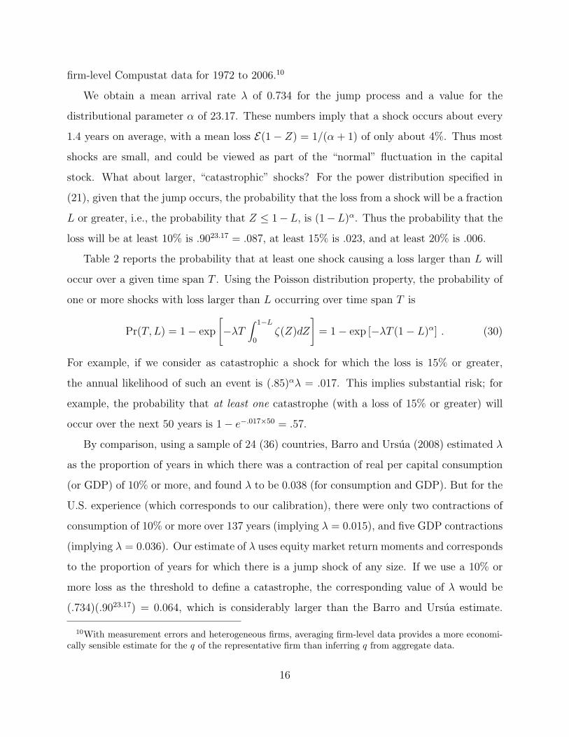
firm-level Compustat data for 1972 to 2006.10

We obtain a mean arrival rate λ of 0.734 for the jump process and a value for the

distributional parameter α of 23.17. These numbers imply that a shock occurs about every

1.4 years on average, with a mean loss E(1− Z) = 1/(α + 1) of only about 4%. Thus most

shocks are small, and could be viewed as part of the “normal” fluctuation in the capital

stock. What about larger, “catastrophic” shocks? For the power distribution specified in

(21), given that the jump occurs, the probability that the loss from a shock will be a fraction

L or greater, i.e., the probability that Z ≤ 1−L, is (1−L)α. Thus the probability that the

loss will be at least 10% is .9023.17 = .087, at least 15% is .023, and at least 20% is .006.

Table 2 reports the probability that at least one shock causing a loss larger than L will

occur over a given time span T . Using the Poisson distribution property, the probability of

one or more shocks with loss larger than L occurring over time span T is

Pr(T, L) = 1− exp

[−λT

∫ 1−L

0ζ(Z)dZ

]= 1− exp [−λT (1− L)α] . (30)

For example, if we consider as catastrophic a shock for which the loss is 15% or greater,

the annual likelihood of such an event is (.85)αλ = .017. This implies substantial risk; for

example, the probability that at least one catastrophe (with a loss of 15% or greater) will

occur over the next 50 years is 1− e−.017×50 = .57.

By comparison, using a sample of 24 (36) countries, Barro and Ursua (2008) estimated λ

as the proportion of years in which there was a contraction of real per capital consumption

(or GDP) of 10% or more, and found λ to be 0.038 (for consumption and GDP). But for the

U.S. experience (which corresponds to our calibration), there were only two contractions of

consumption of 10% or more over 137 years (implying λ = 0.015), and five GDP contractions

(implying λ = 0.036). Our estimate of λ uses equity market return moments and corresponds

to the proportion of years for which there is a jump shock of any size. If we use a 10% or

more loss as the threshold to define a catastrophe, the corresponding value of λ would be

(.734)(.9023.17) = 0.064, which is considerably larger than the Barro and Ursua estimate.

10With measurement errors and heterogeneous firms, averaging firm-level data provides a more economi-cally sensible estimate for the q of the representative firm than inferring q from aggregate data.

16

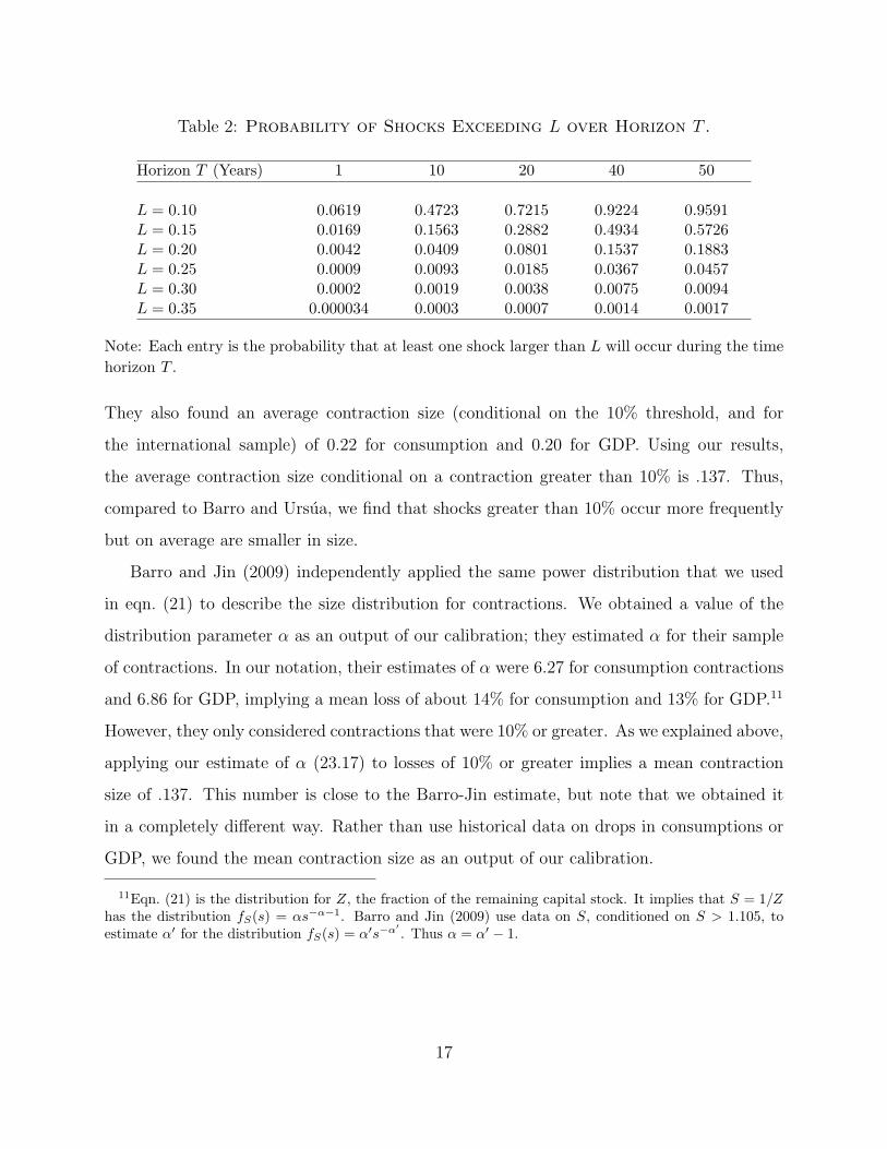
Table 2: Probability of Shocks Exceeding L over Horizon T .

Horizon T (Years) 1 10 20 40 50

L = 0.10 0.0619 0.4723 0.7215 0.9224 0.9591L = 0.15 0.0169 0.1563 0.2882 0.4934 0.5726L = 0.20 0.0042 0.0409 0.0801 0.1537 0.1883L = 0.25 0.0009 0.0093 0.0185 0.0367 0.0457L = 0.30 0.0002 0.0019 0.0038 0.0075 0.0094L = 0.35 0.000034 0.0003 0.0007 0.0014 0.0017

Note: Each entry is the probability that at least one shock larger than L will occur during the timehorizon T .

They also found an average contraction size (conditional on the 10% threshold, and for

the international sample) of 0.22 for consumption and 0.20 for GDP. Using our results,

the average contraction size conditional on a contraction greater than 10% is .137. Thus,

compared to Barro and Ursua, we find that shocks greater than 10% occur more frequently

but on average are smaller in size.

Barro and Jin (2009) independently applied the same power distribution that we used

in eqn. (21) to describe the size distribution for contractions. We obtained a value of the

distribution parameter α as an output of our calibration; they estimated α for their sample

of contractions. In our notation, their estimates of α were 6.27 for consumption contractions

and 6.86 for GDP, implying a mean loss of about 14% for consumption and 13% for GDP.11

However, they only considered contractions that were 10% or greater. As we explained above,

applying our estimate of α (23.17) to losses of 10% or greater implies a mean contraction

size of .137. This number is close to the Barro-Jin estimate, but note that we obtained it

in a completely different way. Rather than use historical data on drops in consumptions or

GDP, we found the mean contraction size as an output of our calibration.

11Eqn. (21) is the distribution for Z, the fraction of the remaining capital stock. It implies that S = 1/Zhas the distribution fS(s) = αs−α−1. Barro and Jin (2009) use data on S, conditioned on S > 1.105, toestimate α′ for the distribution fS(s) = α′s−α

′. Thus α = α′ − 1.

17

3.5 Catastrophic Insurance Premium.

Our model solution also implies the equilibrium price of every possible insurance claim:

p(Z) = λZ−γζ(Z) (31)

where ζ(Z) is the probability density function for the recovery fraction Z, so that λζ(Z) is

the conditional arrival intensity of a shock that destroys a fraction (1 − Z) of the capital

stock. Eqn. (31) gives the payment rate that the CIS buyer must make to insure against

a shock with loss fraction (1 − Z); should that shock occur, the buyer would receive one

unit of the consumption good. Not surprisingly, the higher the arrival rate of a shock with

survival fraction Z, λζ(Z), the higher the corresponding CIS payment. The multiplier Z−γ

in eqn. (31) is the marginal rate of substitution between pre-jump and post-jump values, and

measures the insurance risk premium; the higher is γ and the bigger is the loss (the lower is

Z), the more expensive is the insurance.

Using eqn. (21) for the probability density function that governs the recovery fraction

Z, we can calculate the cost of insuring against any particular risk. Recall that E(Zn) =

α/(α + n). Thus for each CIS with survival fraction Z, the required payment is:

p(Z) = λαZα−γ−1 . (32)

For example, to obtain the cost of insuring against a shock that results in losing a fraction

L or more of the capital stock (i.e., 1− Z ≥ L), the required payment per unit of capital is∫ 1−L

0(1− Z)p(Z)dZ = λα

[(1− L)α−γ

α− γ− (1− L)α−γ+1

α− γ + 1

]. (33)

Thus to obtain the required payment per unit of capital to insure against any size shock, just

set L = 0 in eqn. (33). Note that unlike the existing catastrophic insurance literature, we

obtain the insurance premium in a general equilibrium setting. Also, observe from eqn. (33)

that the CIS payment depends only on risk aversion γ, the parameters describing shocks, i.e.,

λ and α, and the lower bound L of the loss insurance. The CIS payment does not depend on

the EIS ψ and the discount rate ρ, for example, because these parameters do not describe

the characteristics of or attitudes toward risk.

18

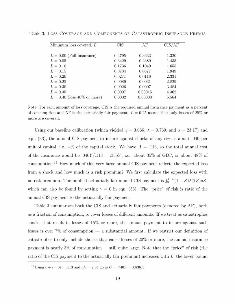
Table 3: Loss Coverage and Components of Catastrophic Insurance Premia

Minimum loss covered, L CIS AF CIS/AF

L = 0.00 (Full insurance) 0.4795 0.3633 1.320L = 0.05 0.3429 0.2389 1.435L = 0.10 0.1736 0.1049 1.655L = 0.15 0.0734 0.0377 1.949L = 0.20 0.0271 0.0116 2.331L = 0.25 0.0089 0.0031 2.829L = 0.30 0.0026 0.0007 3.484L = 0.35 0.0007 0.00015 4.362L = 0.40 (loss 40% or more) 0.0002 0.00003 5.564

Note: For each amount of loss coverage, CIS is the required annual insurance payment as a percentof consumption and AF is the actuarially fair payment. L = 0.25 means that only losses of 25% ormore are covered.

Using our baseline calibration (which yielded γ = 3.066, λ = 0.739, and α = 23.17) and

eqn. (33), the annual CIS payment to insure against shocks of any size is about .040 per

unit of capital, i.e., 4% of the capital stock. We have A = .113, so the total annual cost

of the insurance would be .040Y/.113 = .355Y , i.e., about 35% of GDP, or about 48% of

consumption.12 How much of this very large annual CIS payment reflects the expected loss

from a shock and how much is a risk premium? We first calculate the expected loss with

no risk premium. The implied actuarially fair annual CIS payment is∫ 1−L

0 (1− Z)λζ(Z)dZ,

which can also be found by setting γ = 0 in eqn. (33). The “price” of risk is ratio of the

annual CIS payment to the actuarially fair payment.

Table 3 summarizes both the CIS and actuarially fair payments (denoted by AF), both

as a fraction of consumption, to cover losses of different amounts. If we treat as catastrophes

shocks that result in losses of 15% or more, the annual payment to insure against such

losses is over 7% of consumption — a substantial amount. If we restrict our definition of

catastrophes to only include shocks that cause losses of 20% or more, the annual insurance

payment is nearly 3% of consumption — still quite large. Note that the “price” of risk (the

ratio of the CIS payment to the actuarially fair premium) increases with L, the lower bound

12Using c+ i = A = .113 and c/i = 2.84 gives C = .740Y = .0836K.

19

of the loss fraction that is insured. For example, to insure only against catastrophes that

generate a loss of 10% or more, the price of risk is about 1.7. But if insurance is limited to

only those shocks causing losses of 25% or more (i.e. L = 0.25), the annual cost is just under

1% of consumption, while the actuarially fair rate is about 0.3% of consumption, implying

a price of risk of about 2.8. The price of risk is higher in this case because the insurance is

covering larger losses on average and insuring tail risk is expensive.

3.6 The Role of Adjustment Costs.

How important are adjustment costs? To address this question and do welfare calculations,

we use the quadratic adjustment cost function given by eqn. (7). In our baseline calibration,

the resulting value of θ is 12.03, which is determined by eqn. (17): q = 1/φ′(i) = 1/(1− θi).

In our calibration, q = 1.55, i+ c = A, and c/i = 2.84, which pins down θ = 12.03.

To explore the role of adjustment costs, we first review Barro’s (2009) results and then add

adjustment costs to his model. Based on historic “consumption disasters,” Barro estimated

λ to be .017. He set γ = 4, and using an empirical distribution for consumption declines,

estimated the three moments E(Z), E(Z1−γ), and E(Z−γ). He also set ψ = 2, ρ = .052,

σ = .02, and A = .174. (Because there are no adjustment costs, only A− ρ can be identified

in Barro’s model.)

The first row of the top panel of Table 4 shows this calibration of Barro’s model; there are

no adjustment costs so capital is assumed to be perfectly liquid and q = 1. The calibration

gives a sensible estimate of the risk-free rate r and risk premium rp, but yields a consumption-

investment ratio of only 0.38, whereas the actual ratio is about 3. The rest of the top panel

shows how the results change as the adjustment cost parameter θ in eqn. (7) is increased. The

experiment here is to hold the structural parameters for both preferences and the technology

fixed, change only θ, and then re-solve for the new equilibrium price and quantity allocations.

First, as we increase θ, investment becomes more costly, so i falls and c = A − i increases.

Additionally, q increases because installed capital now earns higher rents in equilibrium.

When θ = 8, both c/i and q roughly match the data. However, r falls below −3%. Basically,

given Barro’s parameter choices (particularly γ and the productivity parameter A) along

20

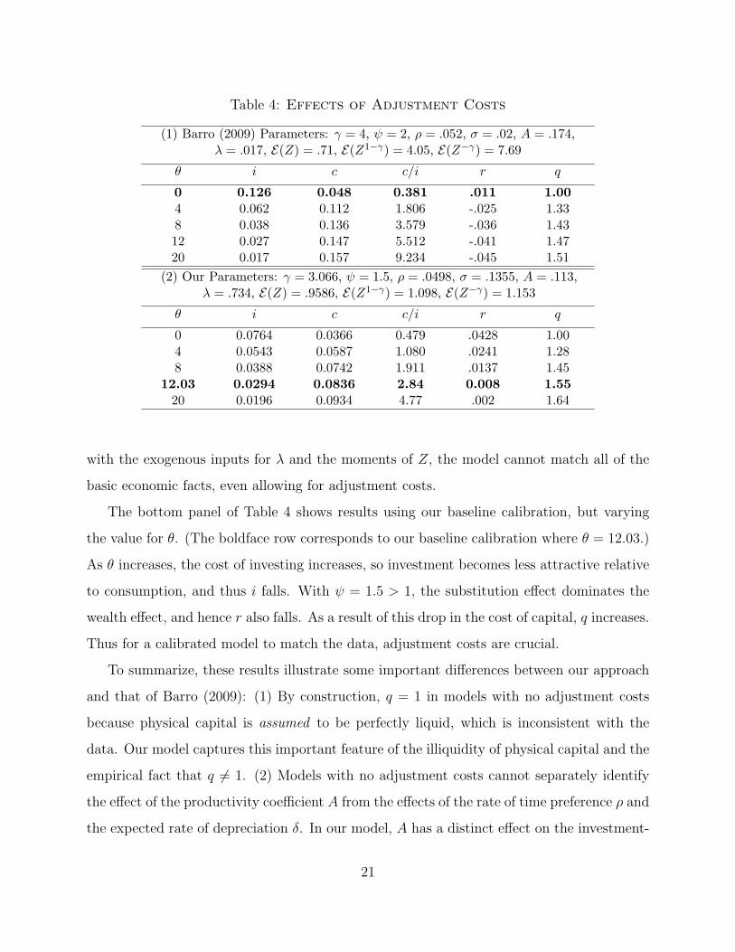
Table 4: Effects of Adjustment Costs

(1) Barro (2009) Parameters: γ = 4, ψ = 2, ρ = .052, σ = .02, A = .174,λ = .017, E(Z) = .71, E(Z1−γ) = 4.05, E(Z−γ) = 7.69

θ i c c/i r q

0 0.126 0.048 0.381 .011 1.004 0.062 0.112 1.806 -.025 1.338 0.038 0.136 3.579 -.036 1.4312 0.027 0.147 5.512 -.041 1.4720 0.017 0.157 9.234 -.045 1.51

(2) Our Parameters: γ = 3.066, ψ = 1.5, ρ = .0498, σ = .1355, A = .113,λ = .734, E(Z) = .9586, E(Z1−γ) = 1.098, E(Z−γ) = 1.153

θ i c c/i r q

0 0.0764 0.0366 0.479 .0428 1.004 0.0543 0.0587 1.080 .0241 1.288 0.0388 0.0742 1.911 .0137 1.45

12.03 0.0294 0.0836 2.84 0.008 1.5520 0.0196 0.0934 4.77 .002 1.64

with the exogenous inputs for λ and the moments of Z, the model cannot match all of the

basic economic facts, even allowing for adjustment costs.

The bottom panel of Table 4 shows results using our baseline calibration, but varying

the value for θ. (The boldface row corresponds to our baseline calibration where θ = 12.03.)

As θ increases, the cost of investing increases, so investment becomes less attractive relative

to consumption, and thus i falls. With ψ = 1.5 > 1, the substitution effect dominates the

wealth effect, and hence r also falls. As a result of this drop in the cost of capital, q increases.

Thus for a calibrated model to match the data, adjustment costs are crucial.

To summarize, these results illustrate some important differences between our approach

and that of Barro (2009): (1) By construction, q = 1 in models with no adjustment costs

because physical capital is assumed to be perfectly liquid, which is inconsistent with the

data. Our model captures this important feature of the illiquidity of physical capital and the

empirical fact that q 6= 1. (2) Models with no adjustment costs cannot separately identify

the effect of the productivity coefficient A from the effects of the rate of time preference ρ and

the expected rate of depreciation δ. In our model, A has a distinct effect on the investment-

21

capital ratio i that differs from the effects of ρ, so that A and ρ can be separately identified.

(3) As noted earlier, Barro’s AK model generates an unrealistically high investment-capital

ratio; our model does not because adjustment costs make investment more expensive.

4 Policy Consequences.

We now turn to the second question raised in the first paragraph of this paper: What is

society’s willingness to pay to reduce the probability or likely impact of catastrophic events?

Our measure of WTP is the maximum permanent consumption tax rate τ that society would

be willing to accept if the resulting stream of government revenue could finance whatever

activities are needed to permanently limit the maximum loss from any catastrophic shock

that might occur to some level L. Of course it might not be feasible to limit the maximum

loss to L with a tax of that size, or it might be possible to achieve this objective with a

smaller tax. In effect, we are examining the “demand side” of public policy — society’s

“reservation price” (maximum tax) for attaining this policy objective.

4.1 Willingness to Pay.

We want to determine the effect of a permanent consumption tax. Given investment It and

output Yt, households pay τ(Yt − It) to the government and consume the remainder:

Ct = (1− τ)(Yt − It) . (34)

Suppose that a costly technology exists that could ensure that any shock that occurs would

lead to a loss no greater than L = (1 − Z). That is, the technology would permanently

change the recovery size distribution ζ(Z) to a truncated distribution, given by

ζ(Z; Z) =αZα−1∫ 1

ZαZα−1dZ

=α

1− ZαZα−1 ; Z ≤ Z ≤ 1 . (35)

Here, Z is the minimal level of recovery Z.

Using this truncated distribution, we obtain the optimal investment-capital ratio i as the

solution of the following equation:

A− i =1

φ′(i)

[ρ+ (ψ−1 − 1)

(φ(i)− γσ2

2− λ

1− γE(1− Z1−γ

))], (36)

22

where E is the expectation with respect to the truncated distribution ζ(Z).

How much would households be willing to pay the government to finance such a tech-

nology? Consider two options: (1) the status quo with no taxes and the original recovery

size distribution ζ(Z); and (2) paying a permanent consumption tax at rate τ to adopt the

new technology which changes the distribution ζ(Z) to ζ(Z) given by eqn. (35). Households

would be indifferent if and only if the following condition holds:

V (K; τ) = V (K; 0) , (37)

where V (K; τ) is the household’s value function given by eqns. (76) and (81) with a consump-

tion tax rate τ , and with the optimal investment-capital ratio i for the truncated distribution

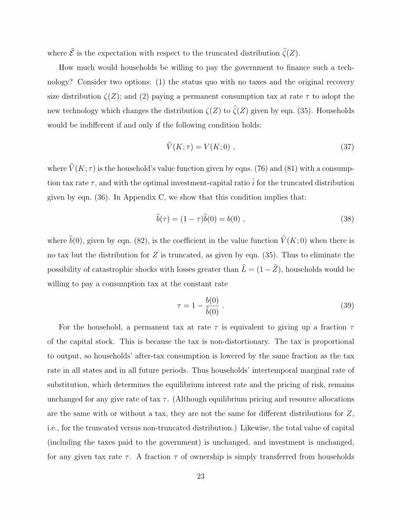
given by eqn. (36). In Appendix C, we show that this condition implies that:

b(τ) = (1− τ)b(0) = b(0) , (38)

where b(0), given by eqn. (82), is the coefficient in the value function V (K; 0) when there is

no tax but the distribution for Z is truncated, as given by eqn. (35). Thus to eliminate the

possibility of catastrophic shocks with losses greater than L = (1− Z), households would be

willing to pay a consumption tax at the constant rate

τ = 1− b(0)

b(0). (39)

For the household, a permanent tax at rate τ is equivalent to giving up a fraction τ

of the capital stock. This is because the tax is non-distortionary. The tax is proportional

to output, so households’ after-tax consumption is lowered by the same fraction as the tax

rate in all states and in all future periods. Thus households’ intertemporal marginal rate of

substitution, which determines the equilibrium interest rate and the pricing of risk, remains

unchanged for any give rate of tax τ . (Although equilibrium pricing and resource allocations

are the same with or without a tax, they are not the same for different distributions for Z,

i.e., for the truncated versus non-truncated distribution.) Likewise, the total value of capital

(including the taxes paid to the government) is unchanged, and investment is unchanged,

for any given tax rate τ . A fraction τ of ownership is simply transferred from households

23

Table 5: WTP Tax Calculations

Note: A = .113, r = .008, c/i = 2.84, rp = .066,V = .0211, S = −0.1116, K = 0.137, g = .020, q = 1.55

Maximum Maximum Tax Rate τLoss ψ = 1.0 ψ = 1.5 ψ = 2.0

0 .474 .522 .5600.05 .298 .316 .3290.10 .154 .159 .1620.15 .066 .067 .0670.20 .024 .024 .0240.25 .008 .008 .0080.30 .002 .002 .0020.35 .001 .001 .001

to the government. This key result follows from the recursive homothetic preferences and

equilibrium property that the economy is on a stochastic balanced growth path.13

4.2 Tax Calculations.

Table 5 shows the maximum permanent tax rate on consumption that society would accept

to limit the maximum loss from a jump shock to various levels. The tax rates are shown for

three different values of the EIS ψ, 1.0, 1.5, and 2.0. (Recall that given ρ we can pin down

ψ, but we cannot pin down both ρ and ψ.) The first row, for which the maximum loss is

zero, gives the tax that society would pay to eliminate all jump shocks. That tax rate is very

large, on the order of 50%. But even if we were to limit the impact of shocks to a loss no

greater than 15%, the warranted tax is substantial — close to 7% per year (forever). Shocks

causing losses greater than 25% or 30% are very rare, so the tax is much lower.

To a first-order approximation, the CIS premium for insuring against losses above a par-

ticular percentage is close to the maximum consumption tax society would pay to eliminate

the possibility of such losses. For example, the CIS premium for insuring against losses above

15% is 7.34% of consumption, which is only slightly larger than the corresponding consump-

13We have focused on policies that would limit the maximum loss from a shock, but the results also applyif the tax is used to reduce the likelihood of a shock of any size.

24

tion tax rate. Eliminating or reducing catastrophic risk, however, is fundamentally different

from purchasing insurance since the latter is a zero NPV financial transaction, with no gain

in value. Using tax proceeds to reduce the consequences of catastrophic shocks is a different

way to manage aggregate risk than purchasing insurance because the former changes real

economic activities (consumption and investment) while the latter simply transfers resources

from one party to the other depending on whether the insured event takes place. Using tax

proceeds to reduce the consequences of catastrophic shocks would be a positive NPV project

and thus welfare enhancing if it could be done at a cost lower than the WTP.

For example, suppose a technology existed such that at an annual cost of 2% of con-

sumption, the maximum loss L from shocks could be capped at 15%. As can be seen from

Table 5, consumers could then gain approximately a 6.7%−2% = 4.7% increase in certainty-

equivalent consumption units. In this case, the benefit of a reduction in catastrophic risk

(by capping the loss at 15%) would clearly outweigh the cost.

Note that because our cost-benefit analysis is a general equilibrium one, it is fundamen-

tally different from the standard cost-benefit approach in which an NPV is calculated treating

input prices and the cost of capital as exogenous. The standard approach is adequate for

evaluating the construction of a new bridge, because while the bridge involves a change in

cash flows, there is no change in the cost of capital (i.e., the pricing kernel). But when the

“project” involves a major change in the economy (e.g., reducing catastrophic risk), prices

as well as cash flows change, so the “project” can only be evaluated by comparing its cost

to its WTP, as we have done above. Our model of a production economy with adjustment

costs is a natural framework for general equilibrium cost-benefit analysis.

4.3 Welfare Decomposition.

Our analysis is related to the “cost of business cycle” literature. Beginning with Lucas

(1987), much of that literature has found the welfare gains from eliminating business cycle

risk to be low. An exception is Barro (2009), who found the welfare gains from eliminating

“conventional” business cycle risk — i.e., continuous fluctuations in output — to be very

low, but the gains from eliminating disaster risk (jump risk in our model) to be substantial.

25

Table 6: Welfare Analysis

Note: A = .113, r = .008, c/i = 2.84, rp = .066, g = .020,V = .0211, S = −0.1116, K = 0.137, q = 1.55, ψ = 1.5

Unless otherwise indicated, σ = .1355, λ = 0.734, θ = 12.025

Change from Baseline Maximum Tax Rate τ

λ = 0 .522σ = 0 .441θ = 0 .289

λ = σ = 0 .786σ = θ = 0 .730λ = θ = 0 .804

λ = σ = θ = 0 .986

For comparison to the earlier literature, we use our model to evaluate these welfare gains.

In our model, we measure welfare gains in terms of WTP, i.e., the maximum consumption

tax society would pay to change the economy such that various risks are reduced or elimi-

nated. We therefore calculate the maximum tax rate to eliminate continuous fluctuations in

the capital stock, i.e., to make σ = 0, leaving jump risk unchanged; to eliminate jump risk

(i.e., make λ = 0), leaving σ unchanged; and to make σ = λ = 0. We also want to determine

the welfare implications of adjustment costs (missing in Barro’s analysis), so we repeat these

calculations but also setting the adjustment cost parameter θ = 0. Finally, we calculate the

welfare gain from eliminating adjustment costs, but leaving both σ and λ unchanged.

The results are shown in Table 6. The first row, for λ = 0, corresponds to the first

row of Table 5, and shows a willingness to pay a consumption tax of over 50% to eliminate

jump risk. However, the willingness to pay to eliminate continuous fluctuations (σ = 0),

leaving jump risk unchanged, is almost as large — a 44% tax. This is in stark contrast to

the results of Barro (2009), Lucas (1987) and others. There are two reasons for this. First,

earlier studies use the 2 to 2.5% standard deviation of log changes in consumption as the

value of σ that describes business cycle risk, whereas we estimate σ to be 13.5% based on

stock return data. Second, we include adjustment costs, which make stochastic fluctuations

in the capital stock (whether continuous or jumps) more costly. Indeed, as the third row of

26

Table 6 shows, the willingness to pay to eliminate adjustment costs — leaving both σ and

λ unchanged — is about 29%. The effects of adjustment costs can also be seen from rows 5

and 6. The WTP to eliminate both jump risk and adjustment costs is a tax rate of about

80%, which is much larger than a 52% tax rate society would pay to eliminate only jump

risk. Similarly, the WTP to eliminate both diffusion risk and adjustment costs is a tax rate

of 73%, as opposed to the 44% tax rate society would pay to eliminate only diffusion risk.

Another reason for the high willingness to pay to eliminate stochastic fluctuations (make

σ, λ, or both zero) is that in our model changes in the capital stock are permanent. Per-

centage changes in the (endogenous) growth rate are iid, i.e., there is no mean reversion.

Allowing for catastrophic shocks to be followed by recoveries (so that there is mean reversion

in growth rate changes), e.g., as in Gourio (2008), would reduce the tax rates in Table 6.

5 Concluding Remarks.

We have provided a new framework for evaluating the characteristics of possible catastrophic

events that are national or global in scale, calculating their implications for catastrophic risk

insurance, and evaluating tax policies to limit their magnitude. Rather than use historical

data on declines in consumption or GDP as others have done, we calculated event charac-

teristics as calibration outputs from a general equilibrium model and used aggregate asset

market data. Our framework provides a natural benchmark to quantitatively assess public

policy; it fully incorporates general equilibrium quantity and price adjustments by the pri-

vate sector in anticipation of a policy intervention. And unlike previous studies, our model

also matches the production side of the economy such as the investment-capital ratio, and

generates sensible estimates for Tobin’s q and for the coefficient of relative risk aversion.

We calculated as a “willingness to pay” measure the permanent tax on consumption

that society would accept to limit the maximum loss from a catastrophic shock. For our

calibration, we found that a permanent tax of about 7% would be justified if the resulting

revenues could be used to limit the impact of shocks to a loss no greater than 15% of the

capital stock. Even if the objective was to limit losses to be no greater than 20 or 25%,

27

a tax of one or two percent would be justified — a substantial tax given that it would

be permanent. These results suggest that governments should devote greater resources to

reducing the risk and potential impact of catastrophes, and thereby provide quantitative

support to arguments along these lines made by Allison (2004), Posner (2004), and Parson

(2007), among others. These arguments are especially important given the tendency of

governments (with their short political cycles) to underestimate both the likelihood and

possible impact of catastrophic events and the value of risk mitigation.14

An alternative to a tax is insurance. We have seen (compare Tables 3 and 5) that

the annual payments required to insure against losses of, say, 15% to 25% are close to the

corresponding tax rates. Insurance, however, is a zero-NPV transaction. In contrast, the

use of tax revenues to eliminate or reduce the potential impact of catastrophes is especially

attractive if the required revenue is less than the WTP, making the social NPV of the tax

policy positive.

We estimated that the probability that over the next 50 years we will experience one

or more shocks causing a loss of 15% or more of the capital stock exceeds 50%, and the

probability of one or more shocks causing a loss of 25% or more is about 5%. (See Table 2.)

These estimates apply to “generic” shocks, i.e., of an unspecified nature. For comparison,

here are estimates of the likelihood and possible impact of some specific catastrophic shocks:

Global Warming: A consensus estimate of the increase in global mean temperature

that would be catastrophic is about 7◦C. A summary of 22 climate science studies surveyed

by the Intergovernmental Panel on Climate Change (IPCC) in 2007 puts the probability of

this occurring by the end of the century at around 5%. Weitzman (2009) argues that the

probability distribution is fat-tailed, making the actual probability as high as 10%. What

would be the impact of a catastrophic increase in temperature? Estimates of the effective

reduction in (world) GDP range from 10% to 30%.15

Nuclear Terrorism: Various studies have assessed the likelihood and impact of the

14Our thanks to an anonymous referee for making this point.15See, e.g., Pindyck (2012) and Stern (2007).

28

detonation of one or several nuclear weapons (with the yield of the Hiroshima bomb) in

major cities. At the high end, Allison (2004) puts the probability of this occurring in the

next ten years at about 50%! Others put the probability for the next ten years at 1 to

5%. For a survey, see Ackerman and Potter (2008). What would be the impact? Possibly

a million or more deaths. But the main shock to the capital stock and GDP would be

a reduction in trade and economic activity worldwide, as vast resources would have to be

devoted to averting further events.

Megaviruses: Numerous authors view major pandemics and plagues (including bioter-

rorism) as both likely and having a catastrophic impact, but do not estimate probabilities.

For a range of possibilities, see Byrne (2008). As with nuclear terrorism, the main shock to

GDP would be a reduction in trade, travel, and economic activity worldwide.

Other Catastrophic Risks: Less likely, but certainly catastrophic, events include

nuclear war, gamma ray bursts, an asteroid hitting the Earth, and unforeseen consequences

of nanotechnology. For an overview, see Bostrom and Cirkovic (2008).

In concluding, some caveats are clearly in order. Our model is intentionally simple and

stylized. For example, we solved the social planner’s problem for a representative firm with

a simple AK production technology and adjustment costs, and a representative household

with rational expectations. This is equivalent to a competitive equilibrium with a large

number of identical firms and identical households, with the same production technology

and preferences, so that we ignore heterogeneity among firms and households. And while

our calibrations fit the basic economic aggregates, we do not statistically test the model. We

also characterize catastrophic events in a simple way — a Poisson arrival with a constant

mean arrival rate, and a permanent impact, the size of which is stochastic. On the other

hand, these simplifications make the model highly tractable, and provide insight into the

questions we raised in the Introduction. We believe that our main results and insights are

robust to these simplifying assumptions.

29

Appendix

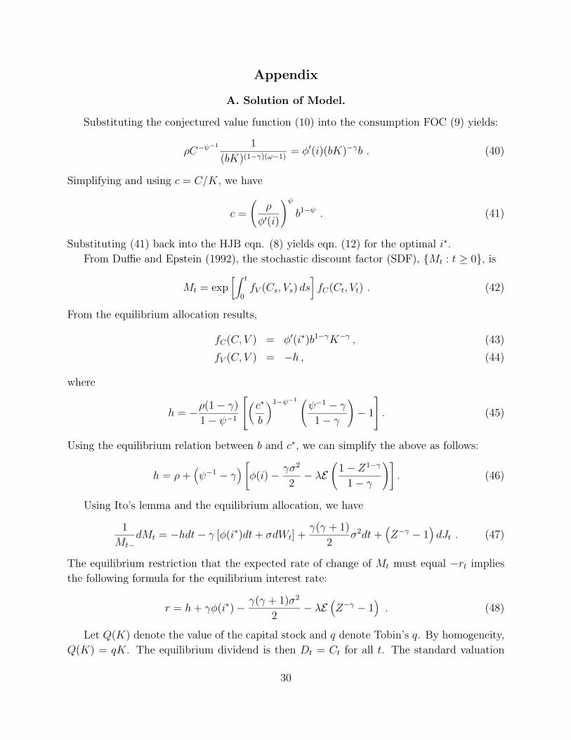
A. Solution of Model.

Substituting the conjectured value function (10) into the consumption FOC (9) yields:

ρC−ψ−1 1

(bK)(1−γ)(ω−1)= φ′(i)(bK)−γb . (40)

Simplifying and using c = C/K, we have

c =

(ρ

φ′(i)

)ψb1−ψ . (41)

Substituting (41) back into the HJB eqn. (8) yields eqn. (12) for the optimal i∗.

From Duffie and Epstein (1992), the stochastic discount factor (SDF), {Mt : t ≥ 0}, is

Mt = exp[∫ t

0fV (Cs, Vs) ds

]fC(Ct, Vt) . (42)

From the equilibrium allocation results,

fC(C, V ) = φ′(i∗)b1−γK−γ , (43)

fV (C, V ) = −h , (44)

where

h = −ρ(1− γ)

1− ψ−1

(c∗b

)1−ψ−1 (ψ−1 − γ

1− γ

)− 1

. (45)

Using the equilibrium relation between b and c∗, we can simplify the above as follows:

h = ρ+(ψ−1 − γ

) [φ(i)− γσ2

2− λE

(1− Z1−γ

1− γ

)]. (46)

Using Ito’s lemma and the equilibrium allocation, we have

1

Mt−dMt = −hdt− γ [φ(i∗)dt+ σdWt] +

γ(γ + 1)

2σ2dt+

(Z−γ − 1

)dJt . (47)

The equilibrium restriction that the expected rate of change of Mt must equal −rt implies

the following formula for the equilibrium interest rate:

r = h+ γφ(i∗)− γ(γ + 1)σ2

2− λE

(Z−γ − 1

). (48)

Let Q(K) denote the value of the capital stock and q denote Tobin’s q. By homogeneity,

Q(K) = qK. The equilibrium dividend is then Dt = Ct for all t. The standard valuation

30

methodology implies that MtDtdt+ d(MtQt) has an instantaneous drift of zero. Using Ito’s

lemma and simplifying yields an equation for q:

c∗

q= ρ−

(1− ψ−1

)φ(i∗) +

γ(1− ψ−1)σ2

2+

λ

1− γE[(ψ−1 − 1

) (Z1−γ − 1

)]. (49)

Using (41) and q = 1/φ′(i∗), we can write the above equation as:

b = ρ

[1 +

(ψ−1 − 1

ρ

)g

] 11−ψ

q , (50)

where g is defined as follows,

g = g − γσ2

2− λ

1− γE(1− Z1−γ

). (51)

The expected rate of return on equity is then

re = ρ+ ψ−1φ(i∗)− γ(ψ−1 − 1)σ2

2+ λE (Z − 1) +

λ

1− γE[(ψ−1 − 1

) (Z1−γ − 1

)]. (52)

Therefore, the aggregate risk premium rp is given by

rp = re − r = γσ2 + λE[(Z − 1)

(1− Z−γ

)]. (53)

B. Moments of Equity Returns.

Here we derive eqns. (23), (24) and (25) for the moments of equity returns. Let k = lnK

and let F (t;x, kt) denote the characteristic function: F (t;x, kt) = Et(eixkT ). From (14),

dkt = αdt+ σdBt − (1− z)dJt , (54)

where z = lnZ and α = (α− 12σ2). Then F (t;x, k) satisfies the differential equation:

αFk +σ2

2Fkk + Ft + λE [F (k + z)− F (k)] = 0 . (55)

We conjecture that

F (t, x, k) = exp [ikG(t, x) +H(t, x)] . (56)

Note that G(T, x) = x and H(T, x) = 0. Substituting (56) for F (t, x, k) into (55) gives

αiG(t, x)− 12σ2G(t, x)2 + [ikGt(t, x) +Ht(t, x)] + λE

[eizG(t,x) − 1

]= 0 . (57)

For the term ikGt(t, x) we have Gt(t, x) = 0 and G(T, x) = x, so G(t, x) = x. For the

remaining terms,

αix− 12σx2 +Ht(t, x) + λE

[eizx − 1

]= 0 . (58)

31

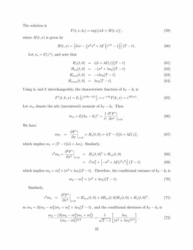
The solution is

F (t, x, kt) = exp [ixk +H(t, x)] , (59)

where H(t, x) is given by

H(t, x) =[αix− 1

2σ2x2 + λE

(eizx − 1

)](T − t) . (60)

Let νn = E(zn), and note that

Hx(t, 0) = i[α + λE(z)](T − t) (61)

Hxx(t, 0) = −(σ2 + λν2)(T − t) (62)

Hxxx(t, 0) = −iλν3(T − t) (63)

Hxxxx(t, 0) = λν4(T − t) (64)

Using kt and k interchangeably, the characteristic function of kT − kt is

F ∗(t, k, x) = Et(eix(kT−kt)

)= e−ixkF (k, x) = eH(t,x) . (65)

Let mn denote the nth (uncentered) moment of kT − kt. Then

mn = Et(kT − kt)n =1

in∂nF ∗

∂xn

∣∣∣∣x=0

. (66)

We have

im1 =∂F ∗

∂x

∣∣∣∣x=0

= Hx(t, 0) = i(T − t)[α + λE(z)] , (67)

which implies m1 = (T − t)(α + λν1). Similarly,

i2m2 =∂2F ∗

∂x2

∣∣∣∣x=0

= Hx(t, 0)2 +Hxx(t, 0) (68)

= i2m21 +

[−σ2 + λE(i2z2)

](T − t) (69)

which implies m2 = m21 + (σ2 +λν2)(T − t) . Therefore, the conditional variance of kT − kt is

m2 −m21 = (σ2 + λν2)(T − t) . (70)

Similarly,

i3m3 =∂3F ∗

∂x3

∣∣∣∣x=0

= Hxxx(t, 0) + 3Hxx(t, 0)Hx(t, 0) +Hx(t, 0)3 , (71)

so m3 = 3(m2 −m21)m1 +m3

1 + λν3(T − t) , and the conditional skewness of kT − kt is

m3 − (3(m2 −m21)m1 +m3

1)

(m2 −m21)3/2

=1√T − t

[λν3

(σ2 + λν2)3/2

]. (72)

32

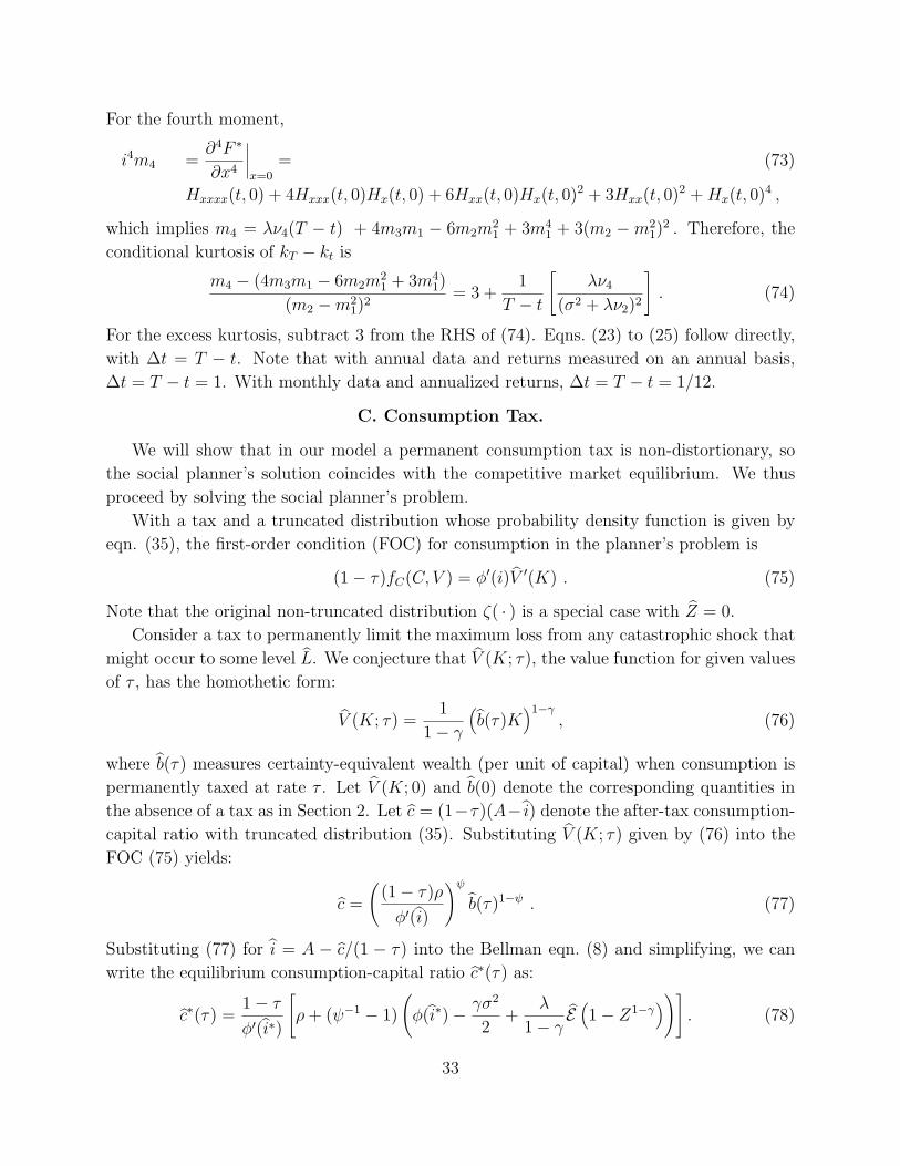
For the fourth moment,

i4m4 =∂4F ∗

∂x4

∣∣∣∣x=0

= (73)

Hxxxx(t, 0) + 4Hxxx(t, 0)Hx(t, 0) + 6Hxx(t, 0)Hx(t, 0)2 + 3Hxx(t, 0)2 +Hx(t, 0)4 ,

which implies m4 = λν4(T − t) + 4m3m1 − 6m2m21 + 3m4

1 + 3(m2 −m21)2 . Therefore, the

conditional kurtosis of kT − kt is

m4 − (4m3m1 − 6m2m21 + 3m4

1)

(m2 −m21)2

= 3 +1

T − t

[λν4

(σ2 + λν2)2

]. (74)

For the excess kurtosis, subtract 3 from the RHS of (74). Eqns. (23) to (25) follow directly,

with ∆t = T − t. Note that with annual data and returns measured on an annual basis,

∆t = T − t = 1. With monthly data and annualized returns, ∆t = T − t = 1/12.

C. Consumption Tax.

We will show that in our model a permanent consumption tax is non-distortionary, so

the social planner’s solution coincides with the competitive market equilibrium. We thus

proceed by solving the social planner’s problem.

With a tax and a truncated distribution whose probability density function is given by

eqn. (35), the first-order condition (FOC) for consumption in the planner’s problem is

(1− τ)fC(C, V ) = φ′(i)V ′(K) . (75)

Note that the original non-truncated distribution ζ( · ) is a special case with Z = 0.

Consider a tax to permanently limit the maximum loss from any catastrophic shock that

might occur to some level L. We conjecture that V (K; τ), the value function for given values

of τ , has the homothetic form:

V (K; τ) =1

1− γ(b(τ)K

)1−γ, (76)

where b(τ) measures certainty-equivalent wealth (per unit of capital) when consumption is

permanently taxed at rate τ . Let V (K; 0) and b(0) denote the corresponding quantities in

the absence of a tax as in Section 2. Let c = (1−τ)(A− i) denote the after-tax consumption-

capital ratio with truncated distribution (35). Substituting V (K; τ) given by (76) into the

FOC (75) yields:

c =

((1− τ)ρ

φ′(i)

)ψb(τ)1−ψ . (77)

Substituting (77) for i = A − c/(1 − τ) into the Bellman eqn. (8) and simplifying, we can

write the equilibrium consumption-capital ratio c∗(τ) as:

c∗(τ) =1− τφ′(i∗)

[ρ+ (ψ−1 − 1)

(φ(i∗)− γσ2

2+

λ

1− γE(1− Z1−γ

))]. (78)

33

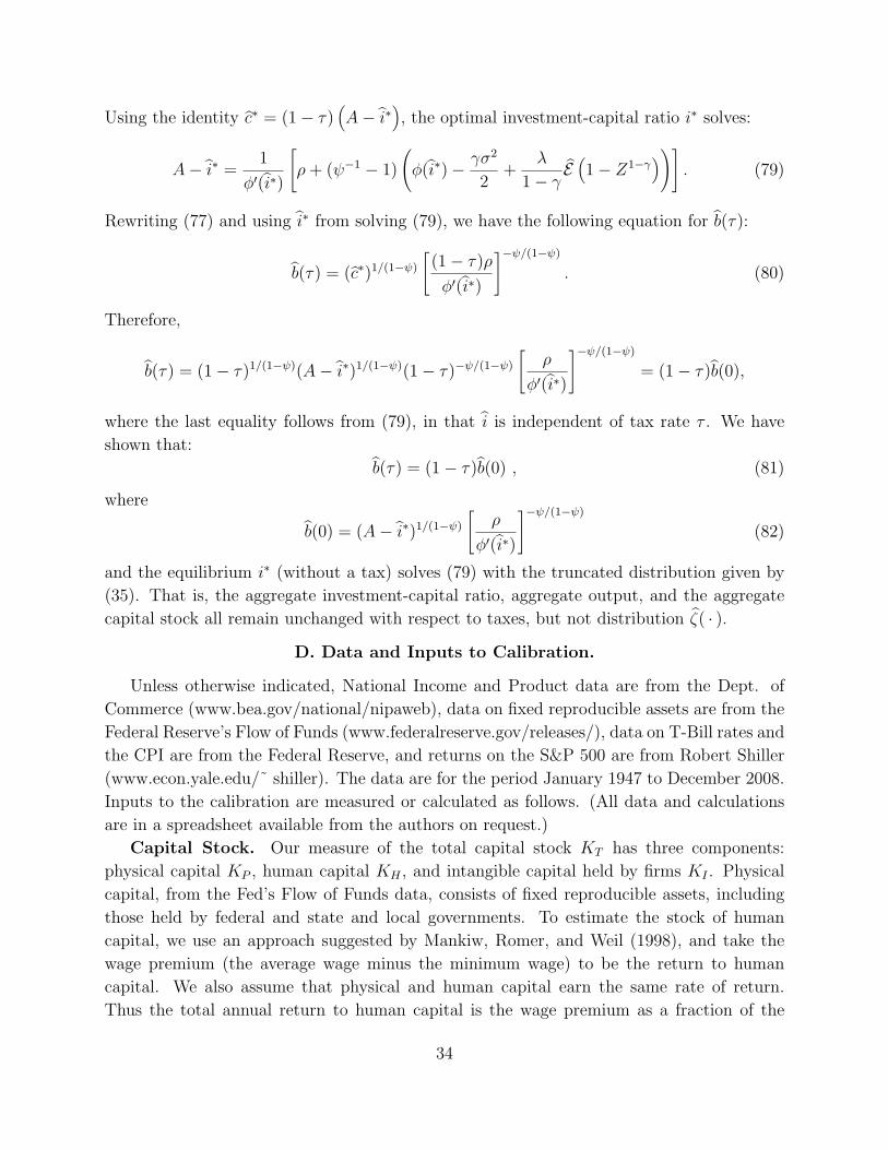
Using the identity c∗ = (1− τ)(A− i∗

), the optimal investment-capital ratio i∗ solves:

A− i∗ =1

φ′(i∗)

[ρ+ (ψ−1 − 1)

(φ(i∗)− γσ2

2+

λ

1− γE(1− Z1−γ

))]. (79)

Rewriting (77) and using i∗ from solving (79), we have the following equation for b(τ):

b(τ) = (c∗)1/(1−ψ)

[(1− τ)ρ

φ′(i∗)

]−ψ/(1−ψ)

. (80)

Therefore,

b(τ) = (1− τ)1/(1−ψ)(A− i∗)1/(1−ψ)(1− τ)−ψ/(1−ψ)

[ρ

φ′(i∗)

]−ψ/(1−ψ)

= (1− τ)b(0),

where the last equality follows from (79), in that i is independent of tax rate τ . We have

shown that:

b(τ) = (1− τ)b(0) , (81)

where

b(0) = (A− i∗)1/(1−ψ)

[ρ

φ′(i∗)

]−ψ/(1−ψ)

(82)

and the equilibrium i∗ (without a tax) solves (79) with the truncated distribution given by

(35). That is, the aggregate investment-capital ratio, aggregate output, and the aggregate

capital stock all remain unchanged with respect to taxes, but not distribution ζ( · ).

D. Data and Inputs to Calibration.

Unless otherwise indicated, National Income and Product data are from the Dept. of

Commerce (www.bea.gov/national/nipaweb), data on fixed reproducible assets are from the

Federal Reserve’s Flow of Funds (www.federalreserve.gov/releases/), data on T-Bill rates and

the CPI are from the Federal Reserve, and returns on the S&P 500 are from Robert Shiller

(www.econ.yale.edu/˜ shiller). The data are for the period January 1947 to December 2008.

Inputs to the calibration are measured or calculated as follows. (All data and calculations

are in a spreadsheet available from the authors on request.)

Capital Stock. Our measure of the total capital stock KT has three components:

physical capital KP , human capital KH , and intangible capital held by firms KI . Physical

capital, from the Fed’s Flow of Funds data, consists of fixed reproducible assets, including

those held by federal and state and local governments. To estimate the stock of human

capital, we use an approach suggested by Mankiw, Romer, and Weil (1998), and take the

wage premium (the average wage minus the minimum wage) to be the return to human

capital. We also assume that physical and human capital earn the same rate of return.

Thus the total annual return to human capital is the wage premium as a fraction of the

34

average wage (about .60 on average) times total compensation of employees. To get the

rate of return on physical capital, we use total capital income (corporate profits including

the capital consumption adjustment, i.e., gross of depreciation, plus rental income, plus

proprietors’ income) as a fraction of the stock of physical capital. That rate of return

(about 7%) is used to capitalize the annual return to human capital.16 For the stock of

intangible capital, we use a weighted average of McGrattan and Prescott’s (2005) estimates

of the intangible capital stock as a fraction of GDP for 1960–69 and 1990–2001. The result

is KI = .68Y . Given annual values for KP , KH , and KI , we calculate annual values for

A = Y/KT and use the average value of A (0.121) as an input to our calibration.

Investment. We need total investment, inclusive of investment in intangible capital,

to measure the consumption-investment ratio C/I. In equilibrium, investment in intangible

capital is given by II = (δI + g)KI , where δI is the depreciation rate for intangible capital

and g is the real GDP growth rate (.02). The BEA’s estimate of the depreciation rate on

R&D is 11%, but McGrattan and Prescott (2005) argue that this rate is too high for most

non-R&D intangible capital. McGrattan and Prescott (2010) estimate the depreciation rate

for intangible capital to be 8%, which is the rate we use. Thus II = .10KI = .068Y .17

Adding this to investment in physical capital yields a consumption-investment ratio of 2.84.

We assume here that investment in human capital occurs through education and is thus part

of measured consumption.

Real Risk-Free Interest Rate and Equity Returns. For the real risk-free rate,

we use monthly data on the nominal 3-month T-bill rate net of the percentage increase

in the CPI for all items. Averaging over the (annualized) monthly numbers yields r =

0.008. For the equity risk premium, we use the monthly total value-weighted return (capital

gains plus dividends) on the S&P500, from CRSP, and subtract the nominal 3-month T-bill

rate. Averaging over the annualized monthly numbers yields rp = 0.066. For the variance,

skewness, and kurtosis of equity returns, we again use the monthly total return on the

S&P500, net of the percentage increase in the CPI.

Real GDP Growth Rate. We use real GDP and population data from the Bureau of

Economic Analysis to compute the annual growth rate of real per-capita GDP. Averaging

over these annual growth rates yields g = .020.

16For comparison, we also calculated the stock of human capital using the results in Jones, Manuelli,Siu, and Stacchetti (2005), who estimated investment in human capital as a fraction of GDP. Assuming thedepreciation rates for human and physical capital are the same, the equilibrium stocks will be in proportionto the investment levels. We obtained similar results (to within 15%) for the stock of human capital.

17This is within the range of the Corrado et al. (2005) estimates of investment in intangible capital.

35

References

Ackerman, Gary, and William C. Potter, “Catastrophic Nuclear Terrorism: A Preventable

Peril,” in Global Catastrophic Risks,” N. Bostrom and M. Cirkovic, editors, Oxford

Univ. Press, 2008.

Allison, Graham, Nuclear Terrorism: The Ultimate Preventable Catastrophe, Henry Holt &

Company, 2004.

Attanasio, Orazio P., and Annette Vissing-Jorgensen, “Stock Market Participation, In-

tertemporal Substitution and Risk Aversion,” American Economic Review, Papers and

Proceedings, May 2003.

Bansal, Ravi, and Amir Yaron, “Risks for the Long Run: A Potential Resolution of Asset

Pricing Puzzles,” Journal of Finance, 2004. 59, 1481–1509.

Barro, Robert J., “Rare Disasters and Asset Markets in the Twentieth Century,” Quarterly

Journal of Economics, 2006, 121, 823–66.

Barro, Robert J., “Rare Disasters, Asset Prices, and Welfare Costs,” American Economic

Review, March 2009, 99, 243-64.

Barro, Robert J., and Tao Jin, “On the Size Distribution of Macroeconomic Disasters,”

NBER Working Paper 15247, August 2009.

Barro, Robert J., Emi Nakamura, Jon Steinsson, and Jose Ursua, “Crises and Recoveries in

an Empirical Model of Consumption Disasters,” unpublished working paper, 2009.

Barro, Robert J., and Jose Ursua, “Macroeconomic Contractions since 1870,” Brookings

Papers on Economic Activity, Spring 2008. 255–335.

Bostrom, Nick, and Milan Cirkovic, editors, Global Catastrophic Risks, Oxford Univ. Press,

(2008).

Byrne, Joseph, editor, Encyclopedia of Pestilence, Pandemics, and Plagues, Greenwood,

2008.

Corrado, Carol, Charles Hulten, and Daniel Sichel, “Measuring Capital and Technology: An

Expanded Framework,” in Corrado, Haltiwanger, and Sichel, eds., Measuring Capital

in the New Economy, University of Chicago Press, 2005.

Duffie, Darrell, and Larry G. Epstein, “Stochastic Differential Utility,” Econometrica, 1992,

60, 353–394.

Epstein, L. G., and S. E. Zin, 1989, “Substitution, risk aversion, and the temporal behavior

of consumption and asset returns: A theoretical framework,” Econometrica, 57, 937-969.

36

Eberly, Janice, Sergio Rebelo, and Nicolas Vincent, “Investment and Value: A Neoclassical

Benchmark,” 2009. Working paper, Northwestern University.

Gabaix, Xavier, “Variable Rare Disasters: An Exactly Solved Framework for Ten Puzzles in

Macro-Finance,” NBER Working Paper No. 13724, January 2008.

Gourio, Francois, “Disasters and Recoveries,” American Economic Review, May 2008, 98,

68–73.

Hall, Robert E., “Intertemporal Substitution in Consumption,” Journal of Political Econ-

omy, April 1988, 96, 339–357.

Hall, Robert E., “Reconciling Cyclical Movements in the Marginal Value of Time and the

Marginal Product of Labor,” Journal of Political Economy, April 2009, 117, 281–323.

Hayashi, Fumio, “Tobin’s marginal q and average q: A neoclassical interpretation. Econo-

metrica 1982, 50, 213-224.

Intergovernmental Panel on Climate Change (IPCC), “Climate Change 2007,” Cambridge

Univ. Press, 2007.

Jermann, Urban J., “Asset Pricing in Production Economies,” Journal of Monetary Eco-

nomics 1998, 41, 257-275.

Jones, Larry E. and Rodolfo E. Manuelli, 2005, “Neoclassical Models of Endogenous Growth:

The Effects of Fiscal Policy, Innovation and Fluctuations,” Handbook of Economic

Growth, ed. Phillippe Aghion and Steven Durlauf, 13-65. Amsterdam: North-Holland.

Jones, Larry E., Rodolfo E. Manuelli, Henry E. Siu, and Ennio Stacchetti, “Fluctuations

in Convex Models of Endogenous Growth, I: Growth Effects,” Review of Economic

Dynamics, 2005, 8, 780–804.

Lucas, Robert E, Jr, Models of Business Cycles, Oxford: Basil Blackwell, 1987.

Mankiw, N. Gregory, David Romer, and David N. Weil, “A Contribution to the Empirics of

Economic Growth,” Quarterly Journal of Economics, May 1992.

McGrattan, Ellen R., and Edward C. Prescott, “Taxes, Regulations, and the Value of U.S.

and U.K. Corporations,” Federal Reserve Bank of Minneapolis Research Staff Report

309, May 2005.

McGrattan, Ellen R., and Edward C. Prescott, “Technology Capital and the U.S. Current

Account,” American Economic Review, Sept. 2010, 100, 1493–1522.

Mehra, Rajnish, and Edward C. Prescott, “The Equity Premium: A Puzzle,” Journal of

Monetary Economics, (1985), 15, 145–161.

37

Parson, Edward A., “The Big One: A Review of Richard Posner’s Catastrophe: Risk and

Response, Journal of Economic Literature, March 2007, 45, 147–164.

Pindyck, Robert S., “Uncertain Outcomes and Climate Change Policy,” Journal of Environ-

mental Economics and Management, forthcoming, 2012.

Posner, Richard A., Catastrophe: Risk and Response, Oxford University Press, 2004.

Rietz, Thomas A., “The Equity Risk Premium: A Solution,” Journal of Monetary Eco-

nomics, (1988), 22, 117–131.

Riddick, Leigh A., and Toni M. Whited, 2009. “The Corporate Propensity to Save,” Journal

of Finance, 64, 1729-1766.

Russett, Bruce, and Miles Lackey, “In the Shadow of the Cloud: If There’s No Tomorrow,

Why Save Today?” Political Science Quarterly, Summer 1987, 102, 259–272.

Russett, Bruce, and Joel Slemrod, “Diminished Expectations of Nuclear War and Increased

Personal Savings: Evidence from Individual Survey Data,” American Economic Review,

Sept. 1993, 83, 1022–1033.

Slemrod, Joel, “Fear of Nuclear War and Intercountry Differences in the Rate of Saving,”

Economic Inquiry, Oct. 1990, 28, 647–657.

Stern, Nicholas, The Economics of Climate Change: The Stern Review, Cambridge Univer-

sity Press, 2007.

Sunstein, Cass R. Worst-Case Scenarios, Harvard University Press, 2007.

Wachter, Jessica, “Can Time-Varying Risk of Rare Disasters Explain Aggregate Stock Mar-

ket Volatility?” NBER Working Paper No. 14386, October 2008.

Weitzman, Martin L., “Subjective Expectations and Asset-Return Puzzles,” American Eco-

nomic Review, Sept. 2007, 97, 1102–1130.

Weitzman, Martin L., “On Modeling and Interpreting the Economics of Catastrophic Climate

Change,” Review of Economics and Statistics, 2009, 91, 1–19.

Weil, Philippe, “Nonexpected Utility in Macroeconomics,” Quarterly Journal of Economics,

1990, 105, 29-42.

38

Appendix E. Decentralized Market Solution.

NOT TO BE PART OF PUBLISHED PAPER

AVAILABLE FROM AUTHORS ON REQUEST.

Here, we provide the decentralized market equilibrium solution. First, we find the rep-

resentative consumer’s optimal consumption, portfolio choice and CIS demand. Second, we

turn to firm value maximization taking prices as given. Finally, we conjecture and verify

equilibrium prices and resource allocation.

Consumer Optimality. Let X denote the consumer’s total marketable wealth and π

the fraction allocated to the market portfolio. For catastrophe with recovery fraction in

(Z,Z + dZ), ξt(Z)Xtdt gives the total demand for the CIS over time period (t, t+ dt). The

total CIS premium payment in the time interval (t, t+ dt) is then(∫ 1

0 ξt(Z)p(Z)dZ)Xtdt.

We conjecture that the cum-dividend return of the market portfolio is given by

dQt +Dtdt

Qt−= µdt+ σdWt − (1− Z)dJt , (83)

where µ is the expected return on the market portfolio (including dividends) but without

the effects of catastrophic risk (and will be determined in equilibrium). When a catastrophe

occurs, the consumer’s wealth changes from Xt− to Xt as follows:

Xt = Xt− − (1− Z)πt−Xt− + ξt−(Z)Xt− . (84)

The consumer’s wealth accumulation is then given by

dXt = r (1− πt−)Xt−dt+ µπt−Xt−dt+ σπt−Xt−dWt − Ct−dt (85)

−(∫ 1

0ξt−(Z)p(Z)dZ

)Xt−dt+ ξt−(Z)Xt−dJt − (1− Z)πt−Xt−dJt .

The first four terms in (85) are standard in classic portfolio choice problems (with no insur-

ance or catastrophes). The last three terms capture the effects of catastrophes on wealth

accumulation. The fifth term is the total CIS premium paid before any catastrophe. The

sixth term gives the CIS payments by the seller to the buyer when a catastrophe occurs.

The last term is the loss of consumer wealth from exposure to the market portfolio.

The HJB equation for the consumer in the decentralized market setting is given by18

0 = maxC,π,ξ( · )

{f(C, J) +

[rX (1− π) + µπX −

(∫ 1

0ξ(Z)p(Z)dZ

)X − C

]J ′(X)

18In writing the HJB equation (8), we use the result that the “normalized” aggregator as defined andderived by Duffie and Epstein (1992) applies to our setting with both jumps and a diffusion. See Benzoni,Collin-Dufresne, and Goldstein, “Explaining Asset Pricing Puzzles Associated with the 1987 Market Crash,”Columbia Univ. working paper, 2010.

39

+1

2σ2π2X2J ′′(X) + λE [J(X − (1− Z)πX + ξ(Z)X)− J(X)]

}. (86)

The FOCs for consumption C, market portfolio allocation as a fraction π of total wealth X,

and the CIS demand ξ(Z) for each Z are respectively:

fC(C, J) = J ′(X) (87)

(µ− r)XJ ′(X) = −σ2πX2J ′′(X) + λE [(1− Z)J ′(X − (1− Z)πX + ξ(Z)X)] (88)

0 = −Xp(Z)J ′(X) + λX [J ′(X − (1− Z)πX + ξ(Z)X)] fZ(Z) . (89)

The last FOC follows from the point-by-point optimization in (86) for the CIS demand and

hence it holds for all levels of Z. Now conjecture that the consumer’s value function is

J(X) =1

1− γ(uX)1−γ , (90)

where u is a constant to be determined. Using the consumption FOC (87) and the conjectured

value function (90), we obtain the following linear consumption rule:

C = ρψu1−ψX . (91)

Imposing the equilibrium outcome in which (1) π = 1; (2) ξ(Z) = 0 for all Z; and (3) the

consumer’s wealth equals the total value of the market portfolio, X = Q, we obtain:

0 = (µ− r)J ′(Q) + σ2QJ ′′(Q)− λE [(1− Z)J ′(ZQ)] (92)

p(Z) = λJ ′(ZQ)

J ′(Q)fZ(Z) (93)

Using these equilibrium conditions, we can simplify the HJB equation as follows:

0 =ρ

1− ψ−1

[(ρ

u

)ψ−1

− 1

]u1−γX1−γ +

(µ− ρψu1−ψ

)(uX)1−γ − γ

2σ2(uX)1−γ

+λE[Z1−γ − 1

] 1

1− γ(uX)1−γ (94)

Eqn. (91) implies c = ρψu1−ψq under the equilibrium condition X = Q = qK. Substi-

tuting c = ρψu1−ψq into (94), we obtain

0 =1

1− ψ−1

(c

q− ρ

)+

(µ− c

q

)− γ

2σ2 + λE

[Z1−γ − 1

] 1

1− γ(95)

Firm Value Maximization. We assume financial markets are perfectly competitive

and M-M holds. While the firm can hold financial positions (e.g., CIS contracts), equilibrium

40

pricing implies that there is no value in doing so. We can thus ignore financial contracts and

only focus on investment I when maximizing firm value, which is independent of financing.

Taking the unique stochastic discount factor (SDF) implied by the equilibrium consumption

process as given, the firm maximizes its value by choosing I to solve:

maxIE[∫ ∞

0

Ms

M0

(AKs − Is) ds], (96)

subject to capital accumulation, the production technology, and the transversality condition.

Using the homogeneity property of our model, we conjecture that the SDF is given by a

geometric Brownian motion with constant drift, constant volatility and proportional jump

for each possible recovery fraction Z, i.e.

dMt = −rMt−dt− ηMt−dWt +Mt−[(Z−γ − 1

)dJt − λE

(Z−γ − 1

)dt]. (97)

The second and the third terms capture diffusion and catastrophic risk respectively. Both

terms are martingales. Note that to make the catastrophe term a martingale, we must

subtract the expected change of M due to all possible catastrophes. Finally, the first term

gives the equilibrium drift of M , which must be −rMt from the no-arbitrage condition.

No arbitrage implies the drift of Mt(AKt − It)dt + d (MtQt) is zero. From Ito’s Lemma

we have the following dynamics for Q(K):

dQ(K) =(

Φ(I,K)QK +1

2QKKσ

2K2)dt+ σKQKdWt + (Q(ZK)−Q(K)) dJt . (98)

Again using Ito’s Lemma, we have

Mt−(AK − I)dt+Mt−

(QKΦ(I,K)dt+

1

2σ2K2QKKdt

)+Q

[−r − λE

(Z−γ − 1

)]Mt−dt

−ηMt−σKQKdt+ λE(Z−γQ(ZK)−Q(K)

)Mt−dt = 0 . (99)

Simplifying the above, we have[r + λE

(Z−γ − 1

)]Q(K) = (AK − I) +QK (Φ(I,K)− ησK) +

1

2σ2K2QKK

+λE(Z−γQ(ZK)−Q(K)

). (100)

The FOC with respect to investment is therefore

1 = ΦI(I,K)QK . (101)

Using the homogeneity assumption, we conjecture that firm value is Q(K) = qK, where

Tobin’s q is to be determined. We can thus simplify (100) as follows:[r + λE

(Z−γ − 1

)]q = (A− i) + q (φ(i)− ησ) + λE

(Z1−γ − 1

)q . (102)

41

The equilibrium dynamic for firm value Qt is then given by

dQt = gQt−dt+ σQt−dWt − (1− Z)Qt−dJt . (103)

where g = φ(i) is the expected growth without the effects of catastrophes.

The FOC (101) can be simplified as follows:

q =1

φ′(i). (104)

Market Equilibrium. We now verify that the conjectured prices and quantities are

consistent with equilibrium market outcomes, and replicate the six key equations (16)-(31)

in the text. First, eqn. (16) follows immediately from the goods market clearing condition,

Y = C + I, and the homogeneity property. Second, eqn. (17) is the FOC for the producer

under homogeneity. Third, we obtain eqn. (18) for consumption by comparing the dynamics

for firm value on the consumer and firm sides, (83) and (103), to obtain the restriction:

µ = φ(i) +c

q. (105)

The expected rate of return (without catastrophes) is φ(i) plus the dividend yield, which is

also the consumption-wealth ratio. Substituting (105) into (95) gives eqn. (18).

Fourth, using the equilibrium consumption and evaluating the SDF via (42), we obtain

the equilibrium interest rate r given by (19) and the equilibrium market price of diffusion

risk η = γσ. Note that the implied interest rate is also consistent with eqn (102).

Fifth, simplifying (92), we have the following result:

0 = (µ− r)− γσ2 − λE[Z−γ(1− Z)

]. (106)

Adding the expected loss due to the catastrophic risk, we obtain the following formula for

the equity risk premium rp:

rp = µ+ λE(1− Z)− r = γσ2 + λE[(1− Z)

(Z−γ − 1

)], (107)

which is eqn. (20). Finally, substituting (90) into (93) gives the CIS insurance premium

p(Z) of eqn. (31). We have verified that the conjectured equilibrium is indeed consistent

with the social planner’s solution.

42