the distributional aspects of social security and social...

�4Social Security and Inequalityover the Life Cycle

Angus Deaton, Pierre-Olivier Gourinchas,and Christina Paxson

4.1 Introduction

This chapter explores the consequences of Social Security reform forthe inequality of consumption across individuals. The basic idea is thatinequality is at least in part the consequence of individual risk in earningsor asset returns. In each period, each person gets a different draw, of earn-ings or of asset returns, so that whenever differences cumulate over time,the members of any group will draw further apart from one another, andinequality will grow. Inequality at a moment of time is the fossilized recordof the history of personal differences in risky outcomes. Any institutionthat shares risk across individuals, the U.S. Social Security system beingthe case in point, will moderate the transmission of individual risk intoinequality, and it is this process that we study in this chapter. Note that weare not concerned here with what has been one of the central issues inSocial Security reform, the distribution between different generations overthe transition. Instead, we are concerned with the equilibrium effects of

Angus Deaton is the Dwight D. Eisenhower Professor of International Affairs and profes-sor of economics and international affairs at the Woodrow Wilson School of Public andInternational Affairs, Princeton University, and a research associate of the National Bureauof Economic Research. Pierre-Olivier Gourinchas is assistant professor of economics atPrinceton University and a faculty research fellow of the National Bureau of EconomicResearch. Christina Paxson is professor of economics and public affairs at the WoodrowWilson School of Public and International Affairs, Princeton University, and a research asso-ciate of the National Bureau of Economic Research.

Angus Deaton and Christina Paxson acknowledge support from the National Institute onAging through a grant to the National Bureau of Economic Research, and from the John D.and Catherine T. MacArthur Foundation within their network on inequality and poverty inbroader perspectives. All the authors are grateful to Martin Feldstein, Laurence J. Kotlikoff,Jeffrey B. Liebman, and James M. Poterba for helpful comments and discussions.

115

different Social Security arrangements on inequality among members ofany given generation.

A concrete and readily analyzed example occurs when the economy iscomposed of autarkic permanent income consumers, each of whom hasan uncertain flow of earnings. Each agent’s consumption follows a mar-tingale (i.e., consumption today equals expected consumption tomorrow),and is therefore the cumulated sum of martingale differences, so that ifshocks to earnings are independent over agents, consumption inequalitygrows with time for any group with fixed membership. The same is true ofasset and income inequality, although not necessarily of earnings inequal-ity: see Deaton and Paxson (1994), who also document the actual growthof income, earnings, and consumption inequality over the life cycle in theUnited States and elsewhere. An insurance arrangement that taxes earn-ings and redistributes the proceeds equally, either in the present or the fu-ture, reduces the rate at which consumption inequality evolves. With com-plete insurance, marginal utilities of different agents move in lockstep, andconsumption inequality remains constant. Social Security pools risks andthus limits the growth of life-cycle inequality. Reducing the share of in-come that is pooled through the Social Security system, as envisaged bysome reform proposals (such as the establishment of individual accountswith different portfolios or different management costs) but not by others(such as setting up a provident fund with a common portfolio and commonmanagement costs) increases the rate at which consumption and incomeinequality evolve over life in a world of permanent-income consumers.Even if inequality is not inherited from one generation to the next, andeach generation starts afresh, partial privatization of Social Security willincrease average inequality. While much of the discussion about limitingportfolio choice in new Social Security arrangements has (rightly) focusedon limiting risk, such restrictions will also have effects on inequality.

Provided the reform is structured so that the poor are made no worseoff, it can be argued that the increase in inequality is of no concern (see,e.g., Feldstein 1998), so that our analysis would be of purely academicinterest. Nevertheless, the fact remains that many people—perhaps mis-taking inequality for poverty—find inequality objectionable, so that it isas well to be aware of the fact if it is the case that an increase in inequalityis likely to be an outcome of Social Security reform. There are also instru-mental reasons for being concerned about inequality; both theoretical andempirical studies implicate inequality in other socially undesirable out-comes, such as low investment in public goods, lower economic growth,and even poor health (Wilkinson 1996).

The paper is organized as follows. Section 4.2 works entirely within theframework of the permanent income hypothesis (PIH). We derive the for-mulas that govern the spread of consumption inequality, and show howinequality is modified by the introduction of a stylized Social Security

116 Angus Deaton, Pierre-Olivier Gourinchas, and Christina Paxson

scheme. The baseline analysis and preliminary results come from Deatonand Paxson (1994), which should be consulted for more details, refine-ments, and reservations, as well as for documentation that consumptioninequality grows over the life cycle, not only in the United States, but atmuch the same rate in Britain and Taiwan. The PIH is convenient becauseit permits closed-form solutions that show explicitly how Social Securityis related to inequality. However, it is not a very realistic model of actualconsumption in the United States, and it embodies assumptions that arefar from obviously appropriate for Social Security analysis—for example,that consumers have unlimited access to credit, and that intertemporaltransfers leaving the present value of lifetime resources unchanged haveno effect on consumption. In consequence, in section 4.3, we considerricher models of consumption and saving that incorporate both precau-tionary motives for saving and borrowing restrictions. These models helpreplicate what we see in the data, which is the tendency of consumers toswitch endogenously from buffer-stock behavior early in life to life-cyclesaving behavior in middle age. The presence of the precautionary motiveand the borrowing constraints breaks the link between consumption andthe present value of lifetime resources, which both complicates and en-riches the analysis of Social Security. Legal restrictions prevent the use ofSocial Security as a collateral for loans, and for at least some people suchrestrictions are likely to be binding.

Solutions to models with precautionary motives and borrowing con-straints are used to document how Social Security systems with differingdegrees of risk sharing affect inequality. We first consider the case in whichall consumers receive the same rate of return on their assets. Our resultsindicate that systems in which there is less sharing of earnings risk—suchas systems of individual accounts—produce higher consumption inequal-ity both before and after retirement. An important related issue is whetherdifferences across consumers in rates of return will contribute to evengreater inequality. Somewhat surprisingly, we find that allowing for fairlysubstantial differences in rates of return across consumers has only modestadditional effects on inequality. The bulk of saving, in the form of bothSocial Security and non–Social Security assets, is done late enough in lifeso that differences in rates of return do not contribute much to consump-tion inequality.

4.2 Social Security and Inequality underthe Permanent Income Hypothesis

Section 4.2.1 introduces the notation and basic algebra of the perma-nent income hypothesis, while section 4.2.2 reproduces from Deaton andPaxson (1994) the basic result on the spread of consumption and incomeinequality over the life cycle. Both subsections are preliminary to the main

Social Security and Inequality over the Life Cycle 117

analysis. Section 4.2.3 introduces a simplified Social Security system in aninfinite horizon model with PIH consumers and shows how a Social Secu-rity tax at rate � reduces the rate of spread of consumption inequality bythe factor (1 � �)2. Section 4.2.4 discusses what happens when there is amaximum to the Social Security tax, and section 4.2.5 extends the modelto deal with finite lives and retirement and shows that the basic resultis unaffected.

4.2.1 Preliminaries: Notation and the Permanent Income Hypothesis

It is useful to begin with the algebra of the PIH; the notation is takenfrom Deaton (1992). Real earnings at time t are denoted yt. Individualconsumption is ct and assets At; when it is necessary to do so we shallintroduce an i suffix to denote individuals. There is a constant real rate ofinterest r. These magnitudes are linked by the accumulation identity

(1) A r A y ct t t t= + + −− − −( )( ) .1 1 1 1

Under certainty equivalence, with rate of time preference equal to r, andan infinite horizon, consumption satisfies the PIH rule, and is equal to thereturn on the discounted present value of earnings and assets:

(2) cr

rA

rr r

E yt tk

k t t k=+

++ +=

∞

+∑1 1

110 ( )

( )

for expectation operator Et, conditional on information available at time t.It is convenient to begin with the infinite horizon case; we deal with thefinite horizon case in section 4.2.5.

That consumption follows a martingale is made evident by manipulationof equation (2):

(3) �cr

r rE E yt t

kk t t t k= ≡

+ +−

=

∞

− +∑�1

110

1( )( ) .

“Disposable” income ydt is defined as earnings plus income from capital:

(4) yr

rA yt

dt t=

++

1.

Saving is the difference between disposable income and consumption,

(5) s y ct td

t= − ,

which enables us to rewrite the PIH rule in equation (2) in the equivalentform (see Campbell 1987):

(6) sr

E ytk

k t t k= −+=

∞

+∑1

11( )

�


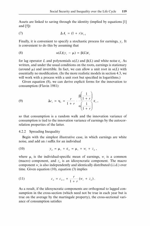
Assets are linked to saving through the identity (implied by equations [1]and [5]):

(7) �A r st t= + −( )1 1

Finally, it is convenient to specify a stochastic process for earnings, yt. Itis convenient to do this by assuming that

(8) � � �( )( ) ( )L y Lt t− = ε

for lag operator L and polynomials �(L) and �(L) and white noise εt. Aswritten, and under the usual conditions on the roots, earnings is stationary(around �) and invertible. In fact, we can allow a unit root in �(L) withessentially no modification. (In the more realistic models in section 4.3, wewill work with a process with a unit root but specified in logarithms.)

Given equation (8), we can derive explicit forms for the innovation toconsumption (Flavin 1981):

(9) �cr

r

r

r

t t t= =+

⋅+

+

�

�

�1

11

11

ε ,

so that consumption is a random walk and the innovation variance ofconsumption is tied to the innovation variance of earnings by the autocor-relation properties of the latter.

4.2.2 Spreading Inequality

Begin with the simplest illustrative case, in which earnings are whitenoise, and add an i suffix for an individual

(10) y w zit i it i t it= + = + +� �ε ,

where �i is the individual-specific mean of earnings, wt is a common(macro) component, and zit is an idiosyncratic component. The macrocomponent wt is also independently and identically distributed (i.i.d.) overtime. Given equation (10), equation (3) implies

(11) c cr

rw zit it t it= +

++−1 1

( ) .

As a result, if the idiosyncratic components are orthogonal to lagged con-sumption in the cross-section (which need not be true in each year but istrue on the average by the martingale property), the cross-sectional vari-ance of consumption satisfies


(12) var var

var

t tz

z

c cr

r

ct r

r

( ) ( )( )

( )( )

= ++

= ++

−1

2 2

2

0

2 2

2

1

1

�

�

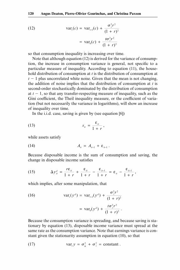
so that consumption inequality is increasing over time.Note that although equation (12) is derived for the variance of consump-

tion, the increase in consumption variance is general, not specific to aparticular measure of inequality. According to equation (11), the house-hold distribution of consumption at t is the distribution of consumption att � 1 plus uncorrelated white noise. Given that the mean is not changing,the addition of noise implies that the distribution of consumption at t issecond-order stochastically dominated by the distribution of consumptionat t � 1, so that any transfer-respecting measure of inequality, such as theGini coefficient, the Theil inequality measure, or the coefficient of varia-tion (but not necessarily the variance in logarithms), will show an increaseof inequality over time.

In the i.i.d. case, saving is given by (see equation [6])

(13) srit

it=+ε

1,

while assets satisfy

(14) A Ait it it= +− −1 1ε .

Because disposable income is the sum of consumption and saving, thechange in disposable income satisfies

(15) �yr

r r r ritd it it it

itit=

++

+−

+= −

+− −ε ε ε

εε

1 1 1 11 1 ,

which implies, after some manipulation, that

(16) var var

var

td

td z

d z

y yr

r

yt r

r

( ) ( )( )

( )( )

.

= ++

= ++

−1

2 2

2

0

2 2

2

1

1

�

�

Because the consumption variance is spreading, and because saving is sta-tionary by equation (13), disposable income variance must spread at thesame rate as the consumption variance. Note that earnings variance is con-stant given the stationarity assumption in equation (10), so that

(17) var constantt zy = + =� ��2 2 .


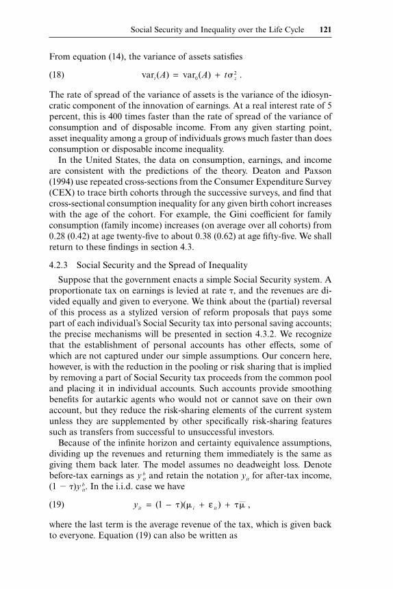
From equation (14), the variance of assets satisfies

(18) var vart zA A t( ) ( ) .= +02�

The rate of spread of the variance of assets is the variance of the idiosyn-cratic component of the innovation of earnings. At a real interest rate of 5percent, this is 400 times faster than the rate of spread of the variance ofconsumption and of disposable income. From any given starting point,asset inequality among a group of individuals grows much faster than doesconsumption or disposable income inequality.

In the United States, the data on consumption, earnings, and incomeare consistent with the predictions of the theory. Deaton and Paxson(1994) use repeated cross-sections from the Consumer Expenditure Survey(CEX) to trace birth cohorts through the successive surveys, and find thatcross-sectional consumption inequality for any given birth cohort increaseswith the age of the cohort. For example, the Gini coefficient for familyconsumption (family income) increases (on average over all cohorts) from0.28 (0.42) at age twenty-five to about 0.38 (0.62) at age fifty-five. We shallreturn to these findings in section 4.3.

4.2.3 Social Security and the Spread of Inequality

Suppose that the government enacts a simple Social Security system. Aproportionate tax on earnings is levied at rate �, and the revenues are di-vided equally and given to everyone. We think about the (partial) reversalof this process as a stylized version of reform proposals that pays somepart of each individual’s Social Security tax into personal saving accounts;the precise mechanisms will be presented in section 4.3.2. We recognizethat the establishment of personal accounts has other effects, some ofwhich are not captured under our simple assumptions. Our concern here,however, is with the reduction in the pooling or risk sharing that is impliedby removing a part of Social Security tax proceeds from the common pooland placing it in individual accounts. Such accounts provide smoothingbenefits for autarkic agents who would not or cannot save on their ownaccount, but they reduce the risk-sharing elements of the current systemunless they are supplemented by other specifically risk-sharing featuressuch as transfers from successful to unsuccessful investors.

Because of the infinite horizon and certainty equivalence assumptions,dividing up the revenues and returning them immediately is the same asgiving them back later. The model assumes no deadweight loss. Denotebefore-tax earnings as y b

it and retain the notation yit for after-tax income,(1 � �)y b

it. In the i.i.d. case we have

(19) yit i it= − + +( )( ) ,1 � � ��ε

where the last term is the average revenue of the tax, which is given backto everyone. Equation (19) can also be written as


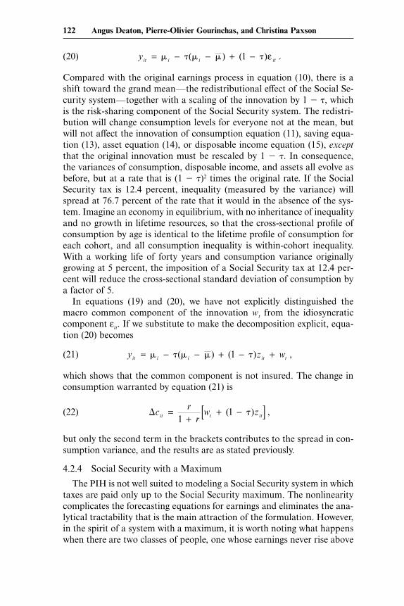
(20) yit i i it= − − + −� � � � �( ) ( ) .1 ε

Compared with the original earnings process in equation (10), there is ashift toward the grand mean—the redistributional effect of the Social Se-curity system—together with a scaling of the innovation by 1 � �, whichis the risk-sharing component of the Social Security system. The redistri-bution will change consumption levels for everyone not at the mean, butwill not affect the innovation of consumption equation (11), saving equa-tion (13), asset equation (14), or disposable income equation (15), exceptthat the original innovation must be rescaled by 1 � �. In consequence,the variances of consumption, disposable income, and assets all evolve asbefore, but at a rate that is (1 � �)2 times the original rate. If the SocialSecurity tax is 12.4 percent, inequality (measured by the variance) willspread at 76.7 percent of the rate that it would in the absence of the sys-tem. Imagine an economy in equilibrium, with no inheritance of inequalityand no growth in lifetime resources, so that the cross-sectional profile ofconsumption by age is identical to the lifetime profile of consumption foreach cohort, and all consumption inequality is within-cohort inequality.With a working life of forty years and consumption variance originallygrowing at 5 percent, the imposition of a Social Security tax at 12.4 per-cent will reduce the cross-sectional standard deviation of consumption bya factor of 5.

In equations (19) and (20), we have not explicitly distinguished themacro common component of the innovation wt from the idiosyncraticcomponent εit. If we substitute to make the decomposition explicit, equa-tion (20) becomes

(21) y z wit i i it t= − − + − +� � � � �( ) ( ) ,1

which shows that the common component is not insured. The change inconsumption warranted by equation (21) is

(22) �cr

rw zit t it=

++ −[ ]1

1( ) ,�

but only the second term in the brackets contributes to the spread in con-sumption variance, and the results are as stated previously.

4.2.4 Social Security with a Maximum

The PIH is not well suited to modeling a Social Security system in whichtaxes are paid only up to the Social Security maximum. The nonlinearitycomplicates the forecasting equations for earnings and eliminates the ana-lytical tractability that is the main attraction of the formulation. However,in the spirit of a system with a maximum, it is worth noting what happenswhen there are two classes of people, one whose earnings never rise above


the Social Security maximum, and one whose earnings never drop belowthe Social Security maximum. Equation (20) still gives after-tax incomefor the poor group, and inequality among them spreads as in the previoussection. For the rich group, after-tax income is

(23) y m

m

it i it i it= − + + + −

++

( )( ) ( )

( ),

1

21

� � � �

��

ε ε

where m is the Social Security maximum, �1 is mean earnings of the poorergroup, and we have assumed that there are equal numbers in the twogroups. (The first term is what is left if tax was paid on everything, thesecond term is the rebate of tax above the maximum, and the last term isthe shared benefit.) Equation (23) can be rewritten as

(24) ym

it i it= −−

+�� ( )

,1

2ε

which makes the straightforward point that those above the maximumno longer participate in the risk sharing, only in the redistribution. As aresult, the Social Security system with the two groups will limit the rateof spread of inequality among the poorer group, but not among the richergroup, although it will bring the two groups closer together than theywould have been in the absence of the system.

4.2.5 Finite Lives with Retirement

With finitely lived consumers we can have a more realistic Social Secu-rity system, in which the taxes are repaid in retirement rather than instan-taneously. One point to note about retirement is that it induces a fall inearnings at the time of retirement, a fall that enters into the determinationof saving (see equation [6]). When there is a unit root in earnings, earningsimmediately prior to retirement have a unit root, and so does the drop inearnings at retirement. In consequence, saving, which must cover this dropin earnings, is no longer stationary but integrated of order one, so thatassets, which are cumulated saving, are integrated of order two. The spreadof inequality in assets is therefore an order of integration faster than thespread of inequality in consumption and disposable income. However, thisseems more a matter of degree than an essential difference.

People work until age R and die at age T. The consumption innovationformula is only slightly different:

(25) � �t t tk

R t

k t t t kcr

r rE E y� = =

+ +−

=

−

− +∑1

110

1( )( ) ,

where the annuity factor �t is given by


(26) � �t T t trr r≡ −

+= + −

− + −11

11

1 1( )( ) .

( )

From equation (25), we can write

(27) c cts

t

s t= +=

−∑00

1� � .

Hence, in the i.i.d. case previously considered,

(28) var vart zs

t

sc cr

r( ) ( )

( ).= +

+ =

−∑0

2

22

0

2

1� �

With the Social Security scheme, after-tax earnings while working is

(29) y

w z

it i it

i t it

= − +

= − + − +

( )( )

( ) ( )( ) .

1

1 1

� �

� � �

ε

With a uniform distribution of ages, the benefits while retired in yearR s are

(30)R w

T RR s� �( )

.+−

+

With certainty equivalence, only the expected present value of this matters(which is a constant given the i.i.d. assumption) so that, once again, al-though the levels of consumption are altered, there is no change to theinnovation of consumption, nor to the rate at which the various inequali-ties spread.

These results would clearly be different with either an autocorrelationstructure of the macro component of earnings such that current innova-tions had information about what will happen in retirement, although thisissue seems hardly worth worrying about; or precautionary motives or bor-rowing restrictions, such that transactions that leave net present valueunaffected can have real effects on the level and profile of consumption.Without quadratic preferences, and without the ability to borrow, we can-not even guarantee the basic result that uncertainty in earnings causesconsumption and income inequality to increase with age. In consequence,we have little choice but to specify a model and to simulate the effects ofalternative Social Security policies, and this is the topic of section 4.3. Ofcourse, it might reasonably be argued that the purpose of Social Securityis not well captured within any of these models, and that present-valueneutral “forced” saving has real effects, not because of precautionary mo-tives or borrowing restrictions, but because people are myopic or otherwiseunable to make sensible retirement plans on their own. We are sympathetic


to the general argument, but have nothing to say about such a case; with-out a more explicit model of behavior, it is not possible to conclude any-thing about the effects of Social Security reform on inequality.

4.3 Social Security with Precautionary Saving or Borrowing Constraints

4.3.1 Describing the Social Security System

When consumers cannot borrow, or when they have precautionary mo-tives for saving, the timing of income affects their behavior. In conse-quence, we need to be more precise about the specification of the SocialSecurity system and its financing. We assume that there is a constant rateof Social Security tax on earnings during the working life, levied at rate �,and that during retirement, the system pays a two-part benefit. The firstpart, G, is a guaranteed floor that is paid to everyone, irrespective of theirearnings or contribution record. The second part, Vi, is individual-specificand depends on the present value of earnings (or contributions) over theworking life. We write Si for the annual payment to individual i after retire-ment, so that

(31) S G V G y r

G y r

i ij

R

ijb R j

j

R

ijR j

= + = + +

= + +

=

−−

=

−−

∑

∑

˜ ( )

( ) ,

�

�

1

1

1

1

1

1

where � �̃/(1 � �). The size of the parameter � determines the extent ofthe link between earnings in work and Social Security payments in retire-ment. When we consider the effects of different Social Security systems oninequality, we shall consider variations in � and G while holding the taxrate � constant. As we shall see below, this is equivalent to devoting a largeror smaller share of Social Security tax revenues to individual accounts.When � is high relative to G (personal saving accounts), the system is rel-atively autarkic, and there is relatively little sharing of risk. Conversely,when G is large and � small (the current system), risk sharing is moreimportant, and we expect inequality to be lower.

The government finances the Social Security system in such a way as tobalance the budget in present-value terms within each cohort. If we usethe date of retirement as the base for discounting, the present value ofgovernment revenues from the Social Security taxes levied on the cohortabout to retire is given by

(32) � �j

R

i

N

ijb R j

j

R

tR jy r Y r

=

−

=

−

=

−−∑ ∑ ∑+ = +

1

1

1 1

1

1 1( ) ( ) ,


where N is the number of people and Yt is aggregate before-tax earningsfor the cohort in year t. This must equal the present value at R of SocialSecurity payments, which is

(33)i

N

j R

TR j

j

R

ijb R jr G y r

= =

−

=

−−∑ ∑ ∑+ + +

1 1

1

1 1( ) ˜ ( ) .�

The budget constraint that revenues equal outlays, that equation (32)equals equation (33), gives a relationship between the three parameters ofthe Social Security system, �, G, and �̃, namely

(34) G yy

rj R

T R j+ =

+=−∑

˜ **

( ),�

�

1

where y* is the average over all consumers of the present value of life-time earnings,

(35) yN

Y rj

R

jR j* ( ) .=

+=

−−∑1

11

1

Equation (34) tells us that we can choose any two of the three parameters,G, � (or �̃), and �, and what is implied for the third. It also makes clearthat, after appropriate scaling, and holding the guarantee fixed, increasesin �—the earnings-related or autarkic part of the system—are equivalentto increases in the rate of the Social Security tax, given that the govern-ment is maintaining within-cohort budget balance.

The link between earnings-related Social Security payments and indi-vidual accounts can be seen more clearly if we reparameterize the system.Suppose that Vi, the earnings-related component of the Social Securitypayment, is funded out of a fraction of Social Security taxes set aside forthe purpose, or equivalently, that a fraction � of the tax is used to build apersonal account, the value of which is used to buy an annuity at retire-ment. Equating the present value of each annuity Vi to the present valueof contributions gives the relationship between � and �,

(36) � =

+=

−∑˜( ) .

�

� j R

TR jr1

Hence, any increase in the earnings-related component of Social Securitythrough an increase in � (or �̃) can be thought of as an increase in thefraction of Social Security taxes sequestered into personal accounts. Equa-tion (34), which constrains the parameters of the Social Security system,can be rewritten in terms of � as

(37) Gy

rj R

T j R= −

+=−∑

* ( )( )

.� 11

�


Note also that the individual Social Security payment in equation (31) canbe rewritten as

(38) Sr

y y ri

j R

T R j j

R

ijb R j=

+− + +

=

− =

−−

∑∑�

( )( ) * ( ) ,

11 1

1

1

� �

so that each person’s Social Security benefits are related to a weightedaverage of their own lifetime earnings and the average lifetime earnings oftheir entire cohort.

If the above scheme were implemented for permanent-income consum-ers who are allowed to borrow and lend at will, the component of SocialSecurity taxes that goes into personal accounts would have no effect onindividual consumption nor, therefore, on its distribution across individu-als. Although the scheme forces people to save, it is fair in present valueterms, and so has no effect on the present value of each individual’s life-time resources. Moreover, although taxes are paid now and benefits re-ceived later, such a transfer can be undone by appropriate borrowing andlending. If the Social Security tax rate is �, and a fraction � is invested ina personal account, it is as if the tax rate were reduced to �(1 � �), andthe rate of increase in the consumption and income variance will be higher.Of course, none of these results hold if consumers are not allowed to bor-row, or if preferences are other than quadratic.

4.3.2 Modeling Consumption Behavior

Although we shall also present results from the permanent income hy-pothesis, our preferred model is one with precautionary motives based onthat in Gourinchas and Parker (2002) and Ludvigson and Paxson (2001),with the addition of retirement and a simple Social Security system. Thespecification and parameters are chosen to provide a reasonable approxi-mation to actual behavior so that, even though it is not possible to deriveclosed-form solutions for the results, we can use simulations to give ussome idea of the effects of the reforms.

Consumers have intertemporally additive isoelastic utility functionsand, as before, they work through years 1 to R � 1, retiring in period Rand dying in period T. The real interest rate is fixed, but the rate of timepreference � is (in general) different from r, so that consumers satisfy thefamiliar Euler equation

(39) c r E ct t t−

+−= + �( ) ( ) ,1 1

where is the inverse of the intertemporal elasticity of substitution and� (1 �)�1. After-tax earnings, where taxes include Social Securitytaxes, evolves according to the (also fairly standard) nonstationary process

(40) ln lny yt t t t= + + −− −1 1� �ε ε ,


which derives from a specification in which log earnings are the sum of arandom walk with drift � and white noise transitory earnings. The quantity� is the parameter of the moving average process for the change in earningsand is an increasing function of the ratio of the variances of the transitoryand random walk components, respectively. Consumers are assumed to beunable to borrow, which requires a modification of equation (39) (see be-low). One reason for this assumption is to mimic the United States, whereit is illegal to borrow against prospective Social Security income. A secondreason is to rule out the possibility that people borrow very large sumsearly in life to finance a declining consumption path over the life cycle.This prohibition could be enforced in other ways, such as the “voluntary”borrowing constraints in Carroll (1997) that result from isoelastic utilitycoupled with a finite probability of zero earnings. We do not find Carroll’sincome process empirically plausible, and it seems simpler to rule out bor-rowing explicitly rather than to choose the form of the earnings process todo so. Our calculations for the permanent income case are made with andwithout borrowing constraints, which will give some idea of the effects ofthe borrowing constraints in the other models.

Our procedure is as follows. Given values for the real interest rate, therate of time preference, the intertemporal elasticity of substitution, themoving average parameter in income growth, and two out of three parame-ters of the Social Security system, we calculate a set of policy functionsfor each year of a forty-year working life. After retirement, there is nofurther uncertainty, and consumption can be solved analytically for eachof the twenty years remaining. We assume that the Social Security systempresented in section 4.3.2 has been in place for a long time, that its parame-ters are fixed, and that people understand how it works, including the gov-ernment’s intertemporal budget constraint. In particular, they understandthe implications of innovations to their earnings for the value of their an-nuities in retirement. We do not require consumers to take into accountthe effects of successive macroeconomic shocks on the size of the SocialSecurity guarantee G. Instead, we assume that the government sets G tothe value that satisfies the budget constraint in expectation for each cohort,and that deficits and surpluses from cumulated macro shocks are passedon to future generations. There are, however, no macro shocks in the simu-lations reported below.

In each period of the working life, the ratio of consumption to earningscan be written as function of three state variables. These are defined asfollows. Define cash on hand xt At yt, which, by equation (1), evolvesduring the working life t � R according to

(41) x r x c yt t t t= + − +− −( )( ) .1 1 1

During retirement, for t � R,


(42) x r x c St t t= + − +− −( )( ) .1 1 1

If wt is the ratio of cash on hand to earnings, and �t the ratio of consump-tion to earnings, then equation (34) becomes, for t � R,

(43) wr w

gtt t

t

=+ −

+− −( )( ),

111 1�

where gt is the ratio of current to lagged income, yt /yt�1. To derive corre-sponding equations for the dynamics of Social Security, define St as thecurrent present value of the annual Social Security payment to which theconsumer would be entitled if he or she earned no more income betweenyear t and retirement. Hence, for t � R,

(44) S G r y rtR t

j

t

jt j= + + +− −

=

−∑( ) ( ) ,( )1 11

�

while for t � R, St is constant and given by equation (31). Noting thatearnings in year R is zero, equation (44) satisfies, for t � R,

(45) S r S Yt t t= + +−( )1 1 �

and is constant thereafter. If we define �t, the ratio of St to current earningsand thus the “Social Security replacement rate,” the corresponding evolu-tion equation is

(46) ��

�tt

t

t

t

S

yr

g= = + +−( ) .1 1

With borrowing constraints, which imply that consumption cannot begreater than cash on hand, or that the consumption ratio be no larger thanthe cash on hand ratio, the Euler equation (39) is modified to

(47) max� � � t t t t tr E g w−

+−

+− −= +[ ]( ) ( ), .1 1 1

We write the consumption ratio �t as a function of the cash on hand ratiowt, the Social Security replacement rate �t, and the current innovation toearnings εt (which is required because, with positive �, high earningsgrowth in one period predicts low earnings growth in the next), and thenuse equation (47) to solve backward for the policy function in each period,starting from the closed-form solution for consumption in the first yearof retirement.

Armed with the policy functions, we simulate lifetime stochastic earn-ings profiles for each of 1,000 people. The logarithm of initial earnings isdrawn from a normal distribution with mean ln (20,000) and a standarddeviation of 0.65, the latter chosen to give an initial Gini coefficient that


roughly corresponds to what we see in the data from the CPS. The drift(expected rate of growth) of earnings is set at 2 percent a year. For anygiven value of the replacement parameter � and the Social Security taxrate �, the corresponding value of the Social Security guarantee G is setfrom equation (34) using actual realized earnings, which, as we have al-ready noted, is potentially problematic if macro shocks are important. Thevalue of G also gives the initial value of �t at the beginning of life. Thecalculated policy functions are then used to simulate life-cycle consump-tion for each of the 1,000 people, and these trajectories are used to assesslifetime inequality as a function of the design of the Social Security system.Different simulations use the same 1,000 sets of earnings realizations, sothat comparisons across Social Security regimes reflect the regime parame-ters and not the specific draws.

4.3.3 Social Security Design and Inequality:Results with Constant Interest Rates

The model is solved under the following assumptions. The interest rater is set at 3 percent, and the rate of time preference at either 3 or 5 percent.The drift of the earnings process is set at 2 percent a year, the movingaverage parameter � to 0.4, and the standard deviation of the innovation(in logs) to be 0.25. The coefficient of relative risk aversion is set to 3, sothat the intertemporal elasticity of substitution is one-third. We also in-clude a certainty equivalent case, with and without borrowing restrictions,in which the rate of interest is set equal to the rate of time preference at 3percent. There are four cases carried through the analysis: (1) isoelasticpreferences, no borrowing, r 0.03, � 0.05; (2) isoelastic preferences,no borrowing, r 0.03, � 0.03; (3) quadratic preferences, no borrowing,r 0.03, � 0.03; and (4), quadratic preferences, borrowing allowed, r 0.03, � 0.03. The Social Security tax rate is set at its current value of12.4 percent of before-tax earnings and there are no other taxes or benefits.The Social Security systems we consider are indexed on the level of theSocial Security guarantee G, which takes the values ($0, $5,000, $10,000,$15,000, $20,000); given the tax rate, these values translate into corre-sponding values for � or, perhaps more revealingly, into values for �, theshare of the tax devoted to personal accounts (1, 0.811, 0.623, 0.434,0.245). These different sets of parameters have quite different implicationsfor the dispersion in Social Security payments among retirees. For ex-ample, our simulation results indicate that with a guarantee of $0, theperson at the 10th percentile (ranked by the present value of lifetime earn-ings) receives an annual Social Security payment of $6,405, in contrast toa payment of $52,639 for the person at the 90th percentile. When the guar-antee is increased to $20,000, this spread declines to $21,569 for the 10thpercentile, and to $32,896 for the 90th.

Figure 4.1 shows the averages over the 1,000 consumers of the simulated


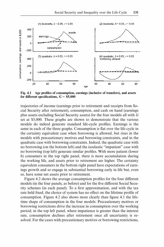
trajectories of income (earnings prior to retirement and receipts from So-cial Security after retirement), consumption, and cash on hand (earningsplus assets excluding Social Security assets) for the four models all with Gset at $5,000. These graphs are shown to demonstrate that the variousmodels do indeed generate standard life-cycle profiles. Earnings is thesame in each of the three graphs. Consumption is flat over the life cycle inthe certainty equivalent case when borrowing is allowed, but rises in themodels with precautionary motives and borrowing constraints, and in thequadratic case with borrowing constraints. Indeed, the quadratic case withno borrowing (on the bottom left) and the isoelastic “impatient” case withno borrowing (top left) generate similar profiles. With more patient (lower�) consumers in the top right panel, there is more accumulation duringthe working life, and assets prior to retirement are higher. The certaintyequivalent consumers in the bottom right panel have expectations of earn-ings growth and so engage in substantial borrowing early in life but, evenso, have some net assets prior to retirement.

Figure 4.2 shows the average consumption profiles for the four differentmodels (in the four panels, as before) and for the five different Social Secu-rity schemes (in each panel). To a first approximation, and with the taxrate held fixed, the choice of system has no effect on the lifetime profile ofconsumption. Figure 4.2 also shows more clearly than figure 4.1 the life-time shape of consumption in the four models: Precautionary motives orborrowing restrictions drive the increase in consumption over the workingperiod; in the top left panel, where impatience is greater than the interestrate, consumption declines after retirement once all uncertainty is re-solved. For the cases with precautionary motives or borrowing restrictions,


Fig. 4.1 Age profiles of consumption, earnings (inclusive of transfers), and assetsfor different specifications, G $5,000

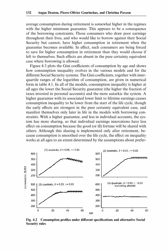
average consumption during retirement is somewhat higher in the regimeswith the higher minimum guarantee. This appears to be a consequenceof the borrowing constraints. Those consumers who draw poor earningsthroughout their lives, and who would like to borrow against their SocialSecurity but cannot, have higher consumption in retirement when theguarantee becomes available. In effect, such consumers are being forcedto save for higher consumption in retirement than they would choose ifleft to themselves. Such effects are absent in the pure certainty equivalentcase where borrowing is allowed.

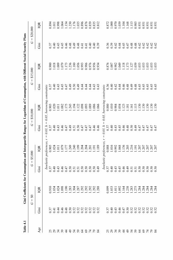
Figure 4.3 plots the Gini coefficients of consumption by age and showshow consumption inequality evolves in the various models and for thedifferent Social Security systems. The Gini coefficients, together with inter-quartile ranges of the logarithm of consumption, are given in numericalform in table 4.1. In all of the models, consumption inequality is higher atall ages the lower the Social Security guarantee (the higher the fraction oftaxes invested in personal accounts) and the more autarkic the system. Ahigher guarantee with its associated lower limit to lifetime earnings causesconsumption inequality to be lower from the start of the life cycle, thoughthe early effects are strongest in the pure certainty equivalent case, andmanifest themselves only later in life in the models with borrowing con-straints. With a higher guarantee, and less in individual accounts, the sys-tem has more sharing, so that individual earnings innovations have lesseffect on consumption because the good (or ill) fortune will be shared withothers. Although this sharing is implemented only after retirement, be-cause consumption is smoothed over the life cycle, the effect on inequalityworks at all ages to an extent determined by the assumptions about prefer-


Fig. 4.2 Consumption profiles under different specifications and alternative SocialSecurity rules

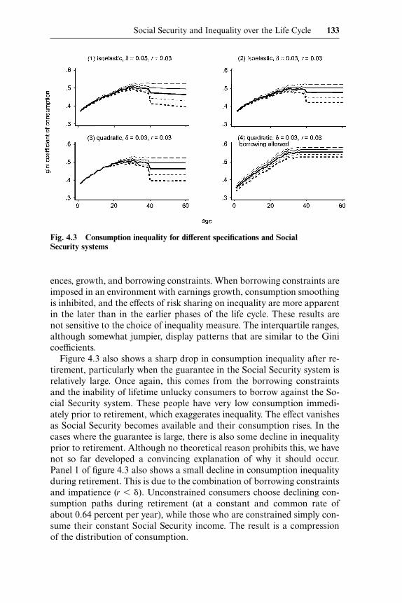
ences, growth, and borrowing constraints. When borrowing constraints areimposed in an environment with earnings growth, consumption smoothingis inhibited, and the effects of risk sharing on inequality are more apparentin the later than in the earlier phases of the life cycle. These results arenot sensitive to the choice of inequality measure. The interquartile ranges,although somewhat jumpier, display patterns that are similar to the Ginicoefficients.

Figure 4.3 also shows a sharp drop in consumption inequality after re-tirement, particularly when the guarantee in the Social Security system isrelatively large. Once again, this comes from the borrowing constraintsand the inability of lifetime unlucky consumers to borrow against the So-cial Security system. These people have very low consumption immedi-ately prior to retirement, which exaggerates inequality. The effect vanishesas Social Security becomes available and their consumption rises. In thecases where the guarantee is large, there is also some decline in inequalityprior to retirement. Although no theoretical reason prohibits this, we havenot so far developed a convincing explanation of why it should occur.Panel 1 of figure 4.3 also shows a small decline in consumption inequalityduring retirement. This is due to the combination of borrowing constraintsand impatience (r � �). Unconstrained consumers choose declining con-sumption paths during retirement (at a constant and common rate ofabout 0.64 percent per year), while those who are constrained simply con-sume their constant Social Security income. The result is a compressionof the distribution of consumption.


Fig. 4.3 Consumption inequality for different specifications and SocialSecurity systems

Tabl

e4.

1G

iniC

oeffi

cien

tsfo

rC

onsu

mpt

ion

and

Inte

rqua

rtile

Ran

ges

for

Log

arit

hmof

Con

sum

ptio

n,w

ith

Diff

eren

tS

ocia

lSec

urit

yP

lans

G

$0G

$5

,000

G

$10,

000

G

$15,

000

G

$20,

000

Age

Gin

iIQ

RG

ini

IQR

Gin

iIQ

RG

ini

IQR

Gin

iIQ

R

Isoe

last

icpr

efer

ence

s,r

0.

03,�

0.

05,b

orro

win

gco

nstr

aint

s25

0.37

0.91

00.

370.

905

0.37

0.90

30.

370.

900

0.37

0.89

429

0.41

1.03

40.

401.

024

0.40

1.02

00.

401.

018

0.40

1.01

134

0.44

1.02

40.

431.

011

0.43

1.01

10.

431.

009

0.43

0.99

839

0.46

1.09

80.

461.

079

0.46

1.08

20.

451.

079

0.45

1.06

444

0.48

1.19

00.

471.

177

0.47

1.17

50.

471.

173

0.46

1.15

449

0.50

1.28

30.

501.

249

0.49

1.24

30.

491.

236

0.48

1.23

054

0.52

1.30

40.

511.

240

0.51

1.19

40.

501.

180

0.49

1.17

659

0.52

1.28

70.

511.

199

0.50

1.12

20.

491.

056

0.48

1.03

564

0.52

1.29

20.

501.

204

0.47

1.09

80.

440.

993

0.41

0.89

669

0.52

1.29

20.

501.

204

0.47

1.09

30.

440.

986

0.41

0.87

674

0.52

1.29

20.

501.

201

0.47

1.08

90.

440.

976

0.40

0.85

979

0.52

1.29

20.

501.

191

0.46

1.08

60.

430.

956

0.40

0.83

584

0.52

1.28

80.

491.

189

0.46

1.06

60.

430.

934

0.39

0.81

2

Isoe

last

icpr

efer

ence

s,r

0.

03,�

0.

03,b

orro

win

gco

nstr

aint

s25

0.37

0.89

90.

370.

888

0.37

0.88

00.

360.

876

0.36

0.87

229

0.40

1.03

30.

401.

016

0.40

1.01

00.

401.

007

0.39

1.00

034

0.43

1.01

10.

430.

992

0.43

0.98

40.

420.

982

0.42

0.97

039

0.46

1.09

20.

451.

068

0.45

1.05

40.

441.

049

0.44

1.03

944

0.47

1.16

40.

461.

136

0.46

1.12

30.

461.

118

0.45

1.10

449

0.50

1.23

80.

491.

205

0.48

1.18

10.

481.

173

0.47

1.16

854

0.52

1.28

30.

511.

216

0.50

1.16

10.

491.

127

0.48

1.11

359

0.52

1.27

50.

511.

191

0.49

1.11

50.

481.

039

0.48

0.98

564

0.52

1.28

40.

501.

207

0.47

1.13

00.

451.

033

0.42

0.93

169

0.52

1.28

40.

501.

207

0.47

1.13

00.

451.

033

0.42

0.93

174

0.52

1.28

40.

501.

207

0.47

1.13

00.

451.

033

0.42

0.93

179

0.52

1.28

40.

501.

207

0.47

1.13

00.

451.

033

0.42

0.93

184

0.52

1.28

40.

501.

207

0.47

1.13

00.

451.

033

0.42

0.93

1

Qua

drat

icpr

efer

ence

s,r

0.

03,�

0.

03,b

orro

win

gco

nstr

aint

s25

0.38

0.91

80.

380.

918

0.38

0.91

80.

380.

918

0.38

0.91

829

0.41

1.05

00.

411.

050

0.41

1.05

00.

411.

050

0.41

1.05

034

0.44

1.06

70.

441.

067

0.44

1.06

70.

441.

067

0.44

1.06

739

0.47

1.16

70.

471.

167

0.47

1.16

70.

471.

166

0.47

1.16

544

0.49

1.23

10.

491.

229

0.48

1.22

70.

481.

224

0.48

1.21

849

0.51

1.32

70.

511.

296

0.50

1.29

10.

491.

283

0.49

1.27

654

0.53

1.31

50.

521.

233

0.51

1.17

70.

501.

157

0.49

1.15

259

0.53

1.28

70.

511.

184

0.50

1.09

30.

491.

045

0.48

1.00

964

0.52

1.29

80.

491.

183

0.46

1.05

00.

430.

929

0.39

0.81

569

0.52

1.29

80.

491.

183

0.46

1.05

00.

430.

929

0.39

0.81

574

0.52

1.29

80.

491.

183

0.46

1.05

00.

430.

929

0.39

0.81

579

0.52

1.29

80.

491.

183

0.46

1.05

00.

430.

929

0.39

0.81

584

0.52

1.29

80.

491.

183

0.46

1.05

00.

430.

929

0.39

0.81

5

PIH

:Q

uadr

atic

pref

eren

ces,

r

0.03

,�

0.03

,no

borr

owin

gco

nstr

aint

s25

0.37

0.89

90.

360.

872

0.36

0.84

50.

350.

818

0.34

0.79

229

0.41

1.02

90.

400.

996

0.39

0.96

50.

380.

934

0.37

0.90

334

0.45

1.06

10.

441.

025

0.43

0.99

00.

420.

955

0.41

0.92

239

0.48

1.19

30.

471.

149

0.46

1.10

70.

451.

066

0.44

1.02

644

0.51

1.33

30.

501.

280

0.48

1.22

90.

471.

180

0.46

1.13

349

0.55

1.45

50.

541.

389

0.52

1.32

80.

511.

270

0.50

1.21

554

0.58

1.51

50.

571.

442

0.55

1.37

70.

541.

316

0.53

1.25

859

0.58

1.52

60.

571.

457

0.55

1.38

80.

541.

323

0.53

1.26

264

0.58

1.56

00.

571.

493

0.55

1.42

20.

541.

356

0.53

1.29

469

0.58

1.56

00.

571.

493

0.55

1.42

20.

541.

356

0.53

1.29

474

0.58

1.56

00.

571.

493

0.55

1.42

20.

541.

356

0.53

1.29

479

0.58

1.56

00.

571.

493

0.55

1.42

20.

541.

356

0.53

1.29

484

0.58

1.56

00.

571.

493

0.55

1.42

20.

541.

356

0.53

1.29

4

Sou

rce:

Aut

hors

’cal

cula

tion

s.N

otes

:“G

ini”

refe

rsto

the

Gin

icoe

ffici

entf

orco

nsum

ptio

n.IQ

Ris

the

inte

rqua

rtile

rang

eof

the

loga

rith

mof

cons

umpt

ion.

PIH

isth

epe

rman

enti

ncom

ehy

-po

thes

is.

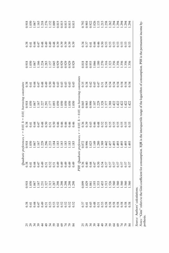
Overall, the results in figure 4.3 and table 4.1 show that as we movefrom one extreme to the other, from putting everything into individual ac-counts and giving no guarantee (a Social Security system than confines itselfto compulsory saving) to a guaranteed floor of $20,000 with only one-fourth of Social Security taxes going to personal accounts, the Gini co-efficient of consumption increases by between 5 and 6 percentage points onaverage over the life cycle, less among the young, and more among the old.This is a large increase, exceeding the increase in consumption inequalityin the United States during the inequality boom from the early to the mid-1980s. For example, the Gini coefficient of total consumption for urbanhouseholds from the U.S. Consumer Expenditure Survey rose from 0.37in 1981 to 0.41 in 1986.

Table 4.2 shows “poverty rates” by age for the different models andSocial Security systems. An individual is defined as being in poverty ifannual consumption is less than $10,000. This poverty threshold was arbi-trarily chosen, but it delivers total poverty rates that are not very differentfrom those in the United States. For example, with G equal to $5,000, thetotal poverty rate is 12.5 percent for the first model. We are more con-cerned with how poverty varies with age than with its level. The age pro-files of poverty are similar for the first three models, in which there areborrowing constraints. Poverty rates decline up to retirement age: Con-strained consumers are more likely to be poor when they are young, andearnings are low. Poverty in retirement depends on the value of the SocialSecurity guarantee. When the guarantee is greater than or equal to thepoverty threshold, poverty in retirement must equal zero. For smaller val-ues of the guarantee, the poverty rate in retirement is generally less thanduring working years. However, in one case—that of isoelastic preferencesand r � �—the poverty rate grows during retirement. In this case, impa-tient consumers reduce consumption over time, and increasingly fall belowthe threshold.

The fourth model, with quadratic preferences and no borrowing con-straints, yields very different results. Poverty rates increase with age up toretirement. Average consumption is constant over the life cycle, and theincreasing dispersion in consumption with age implies that consumers willincreasingly fall below the threshold. Increases in the poverty rate ceaseat retirement. However, Social Security guarantees in excess of the povertythreshold do not eliminate poverty, since (in this model) individuals arefree to borrow against the guarantee during working years. Higher SocialSecurity guarantees do, in fact, reduce poverty, but they do so at all ages,by making lifetime wealth more equal across individuals.

Figure 4.4 compares our simulated patterns of inequality over the lifecycle with those calculated from the data in the CEX and reported in Dea-ton and Paxson (1994). By construction, the life-cycle profile of simulatedearnings inequality is similar to the actual profile. Simulated consumption


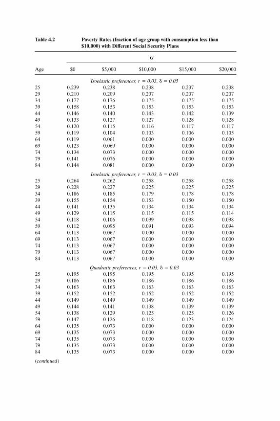
Table 4.2 Poverty Rates (fraction of age group with consumption less than$10,000) with Different Social Security Plans

G

Age $0 $5,000 $10,000 $15,000 $20,000

Isoelastic preferences, r 0.03, � 0.0525 0.239 0.238 0.238 0.237 0.23829 0.210 0.209 0.207 0.207 0.20734 0.177 0.176 0.175 0.175 0.17539 0.158 0.153 0.153 0.153 0.15344 0.146 0.140 0.143 0.142 0.13949 0.133 0.127 0.127 0.128 0.12854 0.120 0.115 0.116 0.117 0.11759 0.119 0.104 0.103 0.106 0.10564 0.119 0.061 0.000 0.000 0.00069 0.123 0.069 0.000 0.000 0.00074 0.134 0.073 0.000 0.000 0.00079 0.141 0.076 0.000 0.000 0.00084 0.144 0.081 0.000 0.000 0.000

Isoelastic preferences, r 0.03, � 0.0325 0.264 0.262 0.258 0.258 0.25829 0.228 0.227 0.225 0.225 0.22534 0.186 0.185 0.179 0.178 0.17839 0.155 0.154 0.153 0.150 0.15044 0.141 0.135 0.134 0.134 0.13449 0.129 0.115 0.115 0.115 0.11454 0.118 0.106 0.099 0.098 0.09859 0.112 0.095 0.091 0.093 0.09464 0.113 0.067 0.000 0.000 0.00069 0.113 0.067 0.000 0.000 0.00074 0.113 0.067 0.000 0.000 0.00079 0.113 0.067 0.000 0.000 0.00084 0.113 0.067 0.000 0.000 0.000

Quadratic preferences, r 0.03, � 0.0325 0.195 0.195 0.195 0.195 0.19529 0.186 0.186 0.186 0.186 0.18634 0.163 0.163 0.163 0.163 0.16339 0.152 0.152 0.152 0.152 0.15244 0.149 0.149 0.149 0.149 0.14949 0.144 0.141 0.138 0.139 0.13954 0.138 0.129 0.125 0.125 0.12659 0.147 0.126 0.118 0.123 0.12464 0.135 0.073 0.000 0.000 0.00069 0.135 0.073 0.000 0.000 0.00074 0.135 0.073 0.000 0.000 0.00079 0.135 0.073 0.000 0.000 0.00084 0.135 0.073 0.000 0.000 0.000

(continued)

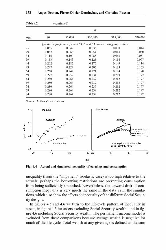
inequality (from the “impatient” isoelastic case) is too high relative to theactuals; perhaps the borrowing restrictions are preventing consumptionfrom being sufficiently smoothed. Nevertheless, the upward drift of con-sumption inequality is very much the same in the data as in the simula-tions, which also show the effects on inequality of the different Social Secur-ity designs.

In figures 4.5 and 4.6 we turn to the life-cycle pattern of inequality inassets, in figure 4.5 for assets excluding Social Security wealth, and in fig-ure 4.6 including Social Security wealth. The permanent income model isexcluded from these comparisons because average wealth is negative formuch of the life cycle. Total wealth at any given age is defined as the sum

Table 4.2 (continued)

G

Age $0 $5,000 $10,000 $15,000 $20,000


Quadratic preferences, r 0.03, � 0.03, no borrowing constraints25 0.055 0.047 0.036 0.030 0.01429 0.082 0.068 0.054 0.043 0.03034 0.116 0.100 0.085 0.068 0.05139 0.153 0.143 0.125 0.114 0.09744 0.202 0.187 0.175 0.149 0.13449 0.247 0.224 0.203 0.183 0.16354 0.260 0.242 0.221 0.194 0.17059 0.277 0.259 0.234 0.209 0.19264 0.280 0.264 0.239 0.212 0.19769 0.280 0.264 0.239 0.212 0.19774 0.280 0.264 0.239 0.212 0.19779 0.280 0.264 0.239 0.212 0.19784 0.280 0.264 0.239 0.212 0.197

Source: Authors’ calculations.

Fig. 4.4 Actual and simulated inequality of earnings and consumption

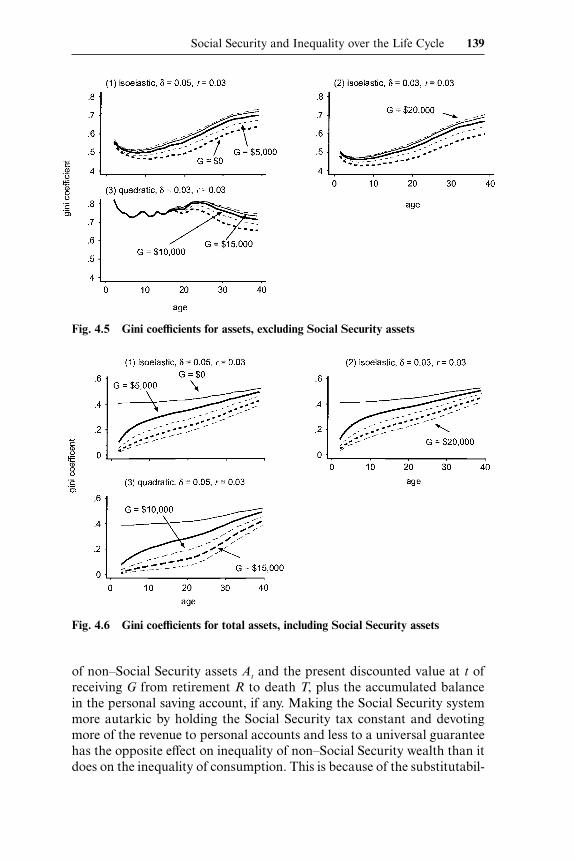
of non–Social Security assets At and the present discounted value at t ofreceiving G from retirement R to death T, plus the accumulated balancein the personal saving account, if any. Making the Social Security systemmore autarkic by holding the Social Security tax constant and devotingmore of the revenue to personal accounts and less to a universal guaranteehas the opposite effect on inequality of non–Social Security wealth than itdoes on the inequality of consumption. This is because of the substitutabil-


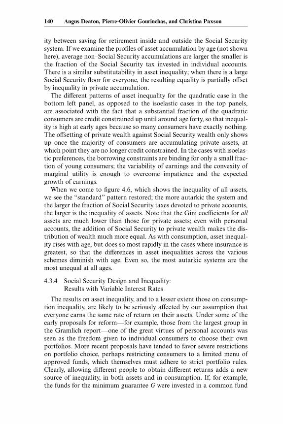
Fig. 4.5 Gini coefficients for assets, excluding Social Security assets

Fig. 4.6 Gini coefficients for total assets, including Social Security assets

ity between saving for retirement inside and outside the Social Securitysystem. If we examine the profiles of asset accumulation by age (not shownhere), average non–Social Security accumulations are larger the smaller isthe fraction of the Social Security tax invested in individual accounts.There is a similar substitutability in asset inequality; when there is a largeSocial Security floor for everyone, the resulting equality is partially offsetby inequality in private accumulation.

The different patterns of asset inequality for the quadratic case in thebottom left panel, as opposed to the isoelastic cases in the top panels,are associated with the fact that a substantial fraction of the quadraticconsumers are credit constrained up until around age forty, so that inequal-ity is high at early ages because so many consumers have exactly nothing.The offsetting of private wealth against Social Security wealth only showsup once the majority of consumers are accumulating private assets, atwhich point they are no longer credit constrained. In the cases with isoelas-tic preferences, the borrowing constraints are binding for only a small frac-tion of young consumers; the variability of earnings and the convexity ofmarginal utility is enough to overcome impatience and the expectedgrowth of earnings.

When we come to figure 4.6, which shows the inequality of all assets,we see the “standard” pattern restored; the more autarkic the system andthe larger the fraction of Social Security taxes devoted to private accounts,the larger is the inequality of assets. Note that the Gini coefficients for allassets are much lower than those for private assets; even with personalaccounts, the addition of Social Security to private wealth makes the dis-tribution of wealth much more equal. As with consumption, asset inequal-ity rises with age, but does so most rapidly in the cases where insurance isgreatest, so that the differences in asset inequalities across the variousschemes diminish with age. Even so, the most autarkic systems are themost unequal at all ages.

4.3.4 Social Security Design and Inequality:Results with Variable Interest Rates

The results on asset inequality, and to a lesser extent those on consump-tion inequality, are likely to be seriously affected by our assumption thateveryone earns the same rate of return on their assets. Under some of theearly proposals for reform—for example, those from the largest group inthe Gramlich report—one of the great virtues of personal accounts wasseen as the freedom given to individual consumers to choose their ownportfolios. More recent proposals have tended to favor severe restrictionson portfolio choice, perhaps restricting consumers to a limited menu ofapproved funds, which themselves must adhere to strict portfolio rules.Clearly, allowing different people to obtain different returns adds a newsource of inequality, in both assets and in consumption. If, for example,the funds for the minimum guarantee G were invested in a common fund


at rate r, as above, but the personal accounts obtained different rates ofreturn for different individuals, either because of their individual portfoliochoices or because of differential management fees, then a move to per-sonal accounts can be expected to increase inequality by more than in thecalculations presented thus far. Alternatively, if the limited menu of fundsoffered different risk-return tradeoffs, and if high earners chose higher re-turns because they are less risk averse, the availability of the menu wouldlikely translate into higher consumption inequality.

It is not obvious how to construct a model with differential asset returnsthat is both realistic and computationally tractable. We have so far consid-ered only one simple case. Personal accounts are invested in one of elevenmutual funds, and consumers must choose among them at the outset ofthe working life. The eleven mutual funds have rates of return from 2.5 to3.5 percent per year. One can think of the funds as having identical (Stan-dard & Poor’s 500) portfolios, but management fees range from zero to 1percentage point; the equilibrium is maintained by differential advertisingand reporting services. We allocate our 1,000 consumers randomly to theeleven mutual funds, with equal probability of receiving any one interestrate; this is a conservative procedure, and inequality would presumably behigher if those with higher earnings were more financially sophisticatedand systematically chose the no-load funds. We assume that consumersare forced to convert their retirement accounts into annuities at retirement(using the interest rate to which they have been assigned), and also thatthe Social Security system gives each consumer a guaranteed amount of$5,000 per year after retirement in addition to the annuity.

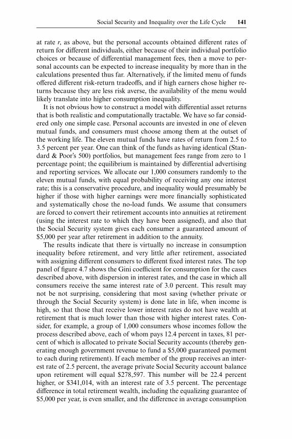
The results indicate that there is virtually no increase in consumptioninequality before retirement, and very little after retirement, associatedwith assigning different consumers to different fixed interest rates. The toppanel of figure 4.7 shows the Gini coefficient for consumption for the casesdescribed above, with dispersion in interest rates, and the case in which allconsumers receive the same interest rate of 3.0 percent. This result maynot be not surprising, considering that most saving (whether private orthrough the Social Security system) is done late in life, when income ishigh, so that those that receive lower interest rates do not have wealth atretirement that is much lower than those with higher interest rates. Con-sider, for example, a group of 1,000 consumers whose incomes follow theprocess described above, each of whom pays 12.4 percent in taxes, 81 per-cent of which is allocated to private Social Security accounts (thereby gen-erating enough government revenue to fund a $5,000 guaranteed paymentto each during retirement). If each member of the group receives an inter-est rate of 2.5 percent, the average private Social Security account balanceupon retirement will equal $278,597. This number will be 22.4 percenthigher, or $341,014, with an interest rate of 3.5 percent. The percentagedifference in total retirement wealth, including the equalizing guarantee of$5,000 per year, is even smaller, and the difference in average consumption


in the first year of retirement for the two interest rates is less than $5,000.This difference is for a spread of one full percentage point; in the exerciseconducted above, most consumers have interest rates between the ex-tremes, so there is even less of an effect on overall inequality.

Even with a much wider spread of returns, there is only a modest effecton inequality. The bottom panel of figure 4.7 shows the case in whichconsumers are distributed over (fixed) rates of return from 1 percent to 7percent, compared with the case in which all get 4 percent. This can bethought of as the case in which consumers make a choice between equitiesand bonds at the beginning of their working careers and may never changethereafter. Because the spread is wider, there is more inequality than be-fore, but the effects are modest compared with the other issues examinedin this chapter.

It is important to note that assigning consumers to different but fixedrates of interest will not necessarily have the same affects as allowing theinterest rate to vary randomly over time for individual consumers. In fu-ture work, we plan to examine how interest rate risk, as opposed to interestrate dispersion, affects inequality.

References

Campbell, John Y. 1987. Does saving anticipate declining labor income? An alter-native test of the permanent income hypothesis. Econometrica 55:1249–73.


Fig. 4.7 The effects on consumption inequality of a distribution of interest rates

Carroll, Christopher. 1997. Buffer-stock saving and the life-cycle permanent in-come hypothesis. Quarterly Journal of Economics 112:1–55.

Deaton, Angus. 1992. Understanding consumption. Oxford, England: ClarendonPress.

Deaton, Angus, and Christina Paxson. 1994. Intertemporal choice and inequality.Journal of Political Economy 102:437–67.

Feldstein, Martin S. 1998. Is income inequality really a problem? In Income in-equality issues and policy options: A symposium sponsored by the Federal ReserveBank of Kansas City, 357–67. N.p.: Federal Reserve Bank of Kansas City.

Flavin, Marjorie. 1981. The adjustment of consumption to changing expectationsabout future income. Journal of Political Economy 89:974–1009.

Gourinchas, Pierre-Olivier, and Jonathan A. Parker. 2002. Consumption over thelife-cycle. Econometrica (forthcoming).

Ludvigson, Sydney, and Christina H. Paxson. 2001. Approximation bias in linear-ized Euler equations. Review of Economics and Statistics 83:242–56.

Wilkinson, Richard. 1996. Unhealthy societies: The afflictions of inequality. Lon-don: Routledge.

Comment James M. Poterba

This is an innovative and important chapter that provides new evidenceon how Social Security programs affect the distribution of lifetime re-sources. The chapter presents an elegant analytical treatment of the issuessurrounding lifetime inequality and retirement transfer programs. It con-siders how a somewhat stylized version of the current U.S. Social Securitysystem would affect the degree of inequality in lifetime consumption, andit also explores how a shift toward an individual accounts Social Securitysystem might affect inequality. The chapter provides a very useful startingpoint for analyzing more complex Social Security arrangements, and manyof my comments will focus on potential directions for such extensions.One very attractive feature of the analysis is the presentation of both Ginicoefficients for consumption inequality as well as summary statistics forthe fraction of the population at different ages that has consumption belowa “poverty line” level.

The chapter begins with an elegant treatment of how a simple SocialSecurity system would affect the inequality of consumption, saving, andassets in a stylized economy. The analysis begins with a very general in-sight. A Social Security system that taxes each worker’s earnings at a fixed

James M. Poterba is the Mitsui Professor of Economics at the Massachusetts Institute ofTechnology, and both a research associate of and director of the public economics researchprogram at the National Bureau of Economic Research.


rate, and then pays each worker a benefit that is tied to the average earn-ings level in the population, reduces the variance of consumption and ofnet-of-tax incomes. If infinitely lived consumers populate the economy,and these consumers save in accordance with the life-cycle hypothesis,then it is possible to derive analytical results for the steady-state varianceof consumption with and without the simplified Social Security system.

While the insights from such a model are quite general, the numericalresults may fail to describe the impact of actual Social Security programsfor two reasons. First, actual Social Security systems do not tax all workersat the same rate, and transfer back a fixed share of economy-wide income.Taxable earnings are often subject to limits, and benefit formulae oftenincorporate progressive elements that transfer larger amounts, per dollarof taxes paid, to low- than to high-earning individuals. Such programmaticdetails would be straightforward to incorporate in a somewhat more de-tailed model of lifetime income and consumption inequality.

The second difficulty with the stylized model in the first part of thechapter is that a substantial body of empirical evidence suggests that manyhouseholds do not behave in accordance with the simple life-cycle hypoth-esis. This concern motivates the second part of the chapter, which uses aricher model of consumer behavior, incorporating precautionary motivesfor saving, to estimate how current and modified Social Security programscould affect consumption inequality. The chapter is careful to considerseveral different specifications of preferences and to illustrate the sensitiv-ity of key findings to various assumptions. The results are presented bothin terms of standard inequality measures, such as the Gini coefficient, andby calculating the fraction of households who experience consumption lev-els below a prespecified threshold.

The chapter yields several findings of broad interest and importance.First, Social Security systems that levy taxes on realized earnings, but pro-vide benefits that depend in part on aggregate earnings, typically reducethe inequality of lifetime consumption. The current defined benefit (DB)system in the United States has some elements of such a system. Programsof this type reduce inequality in consumption both before and after retire-ment, and they can have a particularly large impact on the inequality ofpostretirement consumption when there is a large “guarantee level” thatprovides a consumption floor for Social Security recipients. With such aguarantee, many households will choose not to save at all for retirement,instead relying on the guarantee level to provide their retirement con-sumption.

Second, shifting from a DB Social Security system with a guaranteedbenefit floor to a system of individual accounts will increase consumptioninequality both before and after retirement. The postretirement increasein inequality arises largely from the greater link between preretirementearnings and postretirement resources in individual accounts rather than


redistributive defined-benefit systems. The preretirement increase in con-sumption inequality results in part from the saving adjustments that indi-viduals make in response to the shifting Social Security system. Even ifthe share of earnings devoted to individual accounts was the same as theshare collected by the taxes that finance a DB pension plan, there couldbe endogenous changes in the saving behavior of individuals and in theresulting pattern of preretirement consumption. This is an important in-sight, and one that must be considered in future studies of Social Securityand inequality.

Third, the numerical results suggest that allowing for differences in therates of return earned by different individuals within an individual ac-counts system has a relatively modest impact on the inequality of lifetimeconsumption. This result seems surprising at first, since one would imaginethat greater return variability would result in greater variability of postre-tirement consumption. While variable rates of return work in this direc-tion, they have a modest effect because most retirement saving is done inthe few years before retirement, so the period of time over which differ-ences in returns compound is relatively short. The modest incremental in-crease in consumption inequality is also, to some extent, a reflection of thevery substantial degree of inequality in lifetime income, which translatesinto heterogeneity in postretirement consumption.

The chapter represents an important start on the very substantial taskof modeling how public policies such as Social Security may affect con-sumption inequality. There are many productive directions in which thecurrent analysis could be extended, however, to provide more informationon what might actually happen in a personal accounts retirement system.The remainder of this comment outlines several such directions.

One natural extension is to allow for possible correlation between therate of return that investors earn on their individual accounts and the levelof their lifetime income. There is some evidence from 401(k)-type plans,reported in Poterba and Wise (1998), that higher-income households tendto hold a higher fraction of their 401(k) balances in stocks rather thanbonds. Since stocks have historically provided investors with a higher re-turn than bonds, this raises the prospect that those with higher incomesmay earn better returns on their individual accounts, on average. Such acorrelation would magnify the degree of inequality in retirement resources.It might be particularly important if individuals choose focal values intheir asset allocation, such as 0, 50, or 100 percent stock.

A second potentially useful extension would recognize the potentialfeedback from the Social Security system to the structure of pretax earn-ings. The current analysis treats the pretax income distribution as given.Yet Social Security systems that tax individuals on their earnings, andreturn to them a fraction of the economy-wide average earnings at somefuture date, have incentive effects similar to those of more standard indi-


vidual income taxes. If redistributive DB Social Security systems are rec-ognized as having different incentive effects than individual accounts sys-tems in which individuals can invest a fraction of their earnings, then it ispossible that labor supply would be different under the two systems. Ifhigher tax rates generally discourage labor supply, then one would expecta more compressed distribution of pretax incomes in the DB case than inthe individual accounts case. More generally, the possibility that differentSocial Security systems have different levels of deadweight loss raises ahost of additional issues for analysis, because policies that change the dis-tribution of resources and affect consumption inequality would also affectthe aggregate pool of resources.

A third potential extension would be to recognize that Social Securitybenefits are typically paid to two members of a household, because bothhusbands and wives are eligible to receive benefits. Recent work by Gust-man and Steinmeier (1999) suggests that a very substantial part of the re-distribution that the current Social Security program carries out on anindividual basis is undone when one considers redistribution across house-holds. The households with higher lifetime incomes often have secondaryearners who receive net benefits with larger present discounted values (inrelative terms) than the secondary earners in lower-income couples. Someof this effect operates through differential mortality of secondary earnersin different types of households, and some operates through differences inlifetime earning histories. The central message of this work is that consid-ering couples rather than individuals is a key step for analyzing SocialSecurity policies. The framework developed in this paper could be ex-tended to consider marriage and to create households with two earningsstreams.

A fourth, and particularly ambitious, extension of the current workwould involve using actual earnings histories rather than simulated earn-ings histories to evaluate Social Security redistribution. There is undoubt-edly more information in the history of actual earnings processes than inthe stylized set of earnings histories generated by the stochastic models inthe present chapter. Actual earnings histories are increasingly availablefor research purposes—for example, in conjunction with the Health andRetirement Survey. It would be intriguing to learn whether the patterns ofconsumption inequality that emerge in the current analysis are broadlyconfirmed if the analysis is based on actual earnings experience.

The authors of the present chapter have tackled one of the central issuesin the analysis of Social Security reform. There is little doubt that substan-tive discussions of Social Security reform in the political arena will turnnot only on distributional issues across generations, which have receivedmuch attention in the academic literature, but also on how reform willaffect the distribution of resources within cohorts. This chapter provides avery valuable set of insights for addressing within-cohort redistribution,and it is sure to stimulate further work.


References

Gustman, Alan L., and Thomas L. Steinmeier. 1999. How effective is redistribu-tion under the Social Security benefit formula? Dartmouth College, mimeo-graph.

Poterba, James, and David Wise. 1998. Individual financial decisions in retirementsaving plans and the provision of resources for retirement. In Privatizing SocialSecurity, ed. Martin Feldstein, 363–93. Chicago: University of Chicago Press.

Discussion Summary

Martin Feldstein asked about the relative importance of the timing of con-tributions, because those who contributed early would get the advantageof more years of compound interest. The authors explained that with highwage growth, most income occurs at the end of the life cycle. Conse-quently, almost all contributions are made at the end of the life cycle, andthe impact of compound interest is negligible. The more significant factoris inequality in earnings, not timing of contributions.

John B. Shoven felt that it was important to examine inequality of oppor-tunities, but not necessarily inequality of outcomes. If people are informedand given a broader menu, then the extra choice allows people to max-imize their utility better: It should not be argued that increased choice isterrible because it increases inequality. The authors responded with twopoints. First, most of the inequality comes from earnings inequality, whichis not really chosen in this model. Second, society seems to be concernedabout choices that are made voluntarily, but are very bad decisions ex post.For instance, Teachers Insurance and Annuity Association (TIAA-CREF)has increased the choices, but has limited those choices in some ways be-cause it is worried about people’s voluntarily choosing to become verypoor.

Laurence J. Kotlikoff indicated that the traditional life-cycle picture,high nonasset income followed by lower nonasset income during retire-ment, does not seem to correspond with data in the United States. If SocialSecurity, Medicare, and Medicaid are part of net nonasset income, cohortsgoing through the life cycle now have net nonasset income that risesthrough retirement. The number of people in old age who are borrowingconstrained seems to be important. Hence, an accurate profile of net non-asset income is vital to examining this issue. In addition, if Social Securityis actuarially unfair, then the ceiling on taxable earnings implies that thelower-income classes are affected more severely by this unfairness. Verywealthy people have avoided most of the actuarial penalties of Social Se-curity, and their consumption will be proportionately higher when com-pared to everyone else. In this situation, Social Security might actually


increase consumption inequality. The authors acknowledged the secondobservation, but said it would be difficult to build an earnings ceiling intotheir model for various technical reasons.

Alan Gustman mentioned that when redistribution is examined by fam-ily, about half of the redistribution in the current system disappears. Theamount of redistribution within the family depends on the number of yearsworked by the spouse. While he could understand the difficulties pre-venting the inclusion of these factors in the model, Gustman believed thata large amount of risk sharing and redistribution occurs between familymembers.


the distributional aspects of social security and social...

Documents