the development of annual and peak gas demand · pdf file2.2 annual gas demand in wa ... swis...
TRANSCRIPT
F,
REPORT 4 DECEMBER 2017
THE DEVELOPMENT OF ANNUAL AND PEAK GAS DEMAND FORECASTS FOR THE WESTERN AUSTRALIAN GAS MARKET
Prepared for the Australian Energy Market Operator
Australian Energy Market Operator Gas Demand Forecasts
2.
Marsden Jacob Associates Financial & Economic Consultants ABN 66 663 324 657 ACN 072 233 204 Internet: http://www.marsdenjacob.com.au E-mail: [email protected] Melbourne office: Postal address: Level 4, 683 Burke Road, Camberwell Victoria 3124 AUSTRALIA Telephone: 03 9882 1600 Facsimile: 03 9882 1300 Perth office: Level 1, 220 St Georges Terrace, Perth Western Australia, 6000 AUSTRALIA Telephone: 08 9324 1785 Facsimile: 08 9322 7936 Sydney office: 119 Willoughby Road, Crows Nest New South Wales, 2065 AUSTRALIA Rod Carr 0418 765 393 Authors: Grant Draper [email protected] Phil Jones [email protected] Peter McKenzie [email protected] Hana Ramli [email protected]
This report has been prepared in accordance with the scope of services described in the contract or agreement between Marsden Jacob Associates Pty Ltd ACN 072 233 204 (MJA) and the Client. Any findings, conclusions or recommendations only apply to the aforementioned circumstances and no greater reliance should be assumed or drawn by the Client. Furthermore, the report has been prepared solely for use by the Client and Marsden Jacob Associates accepts no responsibility for its use by other parties.
Copyright © Marsden Jacob Associates Pty Ltd 2017

Australian Energy Market Operator Gas Demand Forecasts
3.
TABLE OF CONTENTS
Introduction .................................................................................................................. 6
1.1 Background ................................................................................................................................. 6
1.2 Scope of Work ............................................................................................................................. 6
1.3 Purpose of this Report ................................................................................................................. 7
1.4 Outline of Report ......................................................................................................................... 7
Gas Use in Western Australia .......................................................................................... 8
2.1 Introduction ................................................................................................................................ 8
2.2 Annual Gas Demand in WA .......................................................................................................... 8
2.3 Peak Day Gas Demand .............................................................................................................. 10
Drivers of Gas Demand in WA ....................................................................................... 11
3.1 GPG in the SWIS ......................................................................................................................... 11
3.1.1 Relationship between GPG Gas Use and Electricity Demand Forecasts ...................................... 12
3.2 Mining ........................................................................................................................................ 13
3.3 Mineral Processing .................................................................................................................... 16
3.4 Industry ...................................................................................................................................... 17
3.5 GPG for NWIS and Regional Centres – Residential and Business Demand ................................... 18
3.6 Other SWIS Gas Demand ........................................................................................................... 19
3.7 Drivers of Segment Growth in GPG Non-SWIS and Other SWIS ................................................. 20
3.7.1 Population Growth .................................................................................................................... 20
3.7.2 Household Income ..................................................................................................................... 22
3.7.3 Economic Drivers ....................................................................................................................... 22
3.7.4 Retail Gas Prices ........................................................................................................................ 23
3.8 Weather .................................................................................................................................... 24
3.9 New Projects ............................................................................................................................. 25
SWIS GPG Gas Use Forecasting Methodology ............................................................... 27
4.1 Key Drivers ................................................................................................................................. 27
4.2 Modelling Approach ................................................................................................................... 27
4.3 Modelling Assumptions ............................................................................................................. 28
4.4 Normalised Load Duration Curve (LDC) for Annual and Monthly Load Forecasts ......................... 31
4.5 Determining Gas Usage on the Peak Gas Days ............................................................................ 31
Annual and Monthly Demand Forecast Methodology for Gas Use Segments ................... 33
5.1 Introduction ............................................................................................................................... 33
5.2 Mineral Processing and Industry Gas Use Segments .................................................................... 33
5.3 Mining ....................................................................................................................................... 34
5.4 GPG for NWIS and Regional Centres – Residential and Business Demand .................................... 35
5.5 Other SWIS ................................................................................................................................ 35
5.6 Gas Shipping (transmission)....................................................................................................... 42
Developing Peak Demand Forecasts ............................................................................. 45
Annual Average Gas Demand Forecasts ........................................................................ 48
7.1 Gas Use Scenarios ..................................................................................................................... 48
7.2 Average Daily Gas Demand Forecasts ........................................................................................ 48
Australian Energy Market Operator Gas Demand Forecasts
4.
Peak Demand Forecasts ............................................................................................... 51
8.1 Summer Peak Demand Forecasts ............................................................................................... 51
8.2 Winter Peak Demand Forecasts ................................................................................................. 54
Appendix One: SWIS GPG Modelling Assumptions ........................................................ 58
A1. Inflation ..................................................................................................................................... 58
A2. Exchange Rates ......................................................................................................................... 58
A3. Environmental Policies .............................................................................................................. 58
A4. Demand and Consumption Forecasts......................................................................................... 59
A5. WEM Plant Retirement Decisions .............................................................................................. 61
A6. Fuel Prices ................................................................................................................................ 61
TABLE OF FIGURES
Figure 1: End User Daily Gas Consumption (TJ/day) .............................................................................................. 10 Figure 2: Operational Consumption Forecasts for the WEM .................................................................................. 13 Figure 3: Average Gas Demand for Iron Ore Mines in WA ...................................................................................... 14 Figure 4: Mining Gas Consumption (Non-SWIS) – TJ/day ...................................................................................... 15 Figure 5: Commodity Price Index and Mining Gas Consumption ............................................................................ 15 Figure 6: Alumina Gas Use in Western Australia .................................................................................................... 16 Figure 7: Alumina Gas Usage Profiles: Historical and Average (2013 to 1017) ......................................................... 17 Figure 8: Gas Consumption by Major Industry Users ............................................................................................. 18 Figure 9: GPG Gas Use (Non-SWIS) ...................................................................................................................... 19 Figure 10: Other Gas Use (SWIS) and Heating Degree Days .................................................................................. 19 Figure 11: WA and SWIS Population...................................................................................................................... 20 Figure 12: WA and SWIS Population Growth Rates ............................................................................................... 21 Figure 13: Population Growth Rate Forecasts ........................................................................................................ 21 Figure 14: Change in Real Per Capita Household Disposable Income in WA ........................................................... 22 Figure 15: State Final Demand - Annual Growth Rates (real) ................................................................................. 23 Figure 16: Retail Gas Price index and WA CPI (annual changes) ............................................................................. 24 Figure 17: Cooling and Heating Degree Days by Calendar Year ............................................................................. 25 Figure 18: PROPHET WEM forecast: Generation by Plant (GWh) .......................................................................... 28 Figure 19: Renewable Investment in the WEM by Scenario (MW) .......................................................................... 30 Figure 20: Load Duration Curve for the SWIS ........................................................................................................ 31 Figure 21: Relationship between Temperature and GPG Gas Use in the WEM – 2013 to 2017 ................................. 32 Figure 22: Non-Specific Mining Gas Use (Non-SWIS) - TJ/day ............................................................................... 34 Figure 23: Predicted Versus Actual Gas Use by Other Segment (SWIS).................................................................. 36 Figure 24: Residential Prices versus Weather Adjusted Consumption Per Capita ................................................... 37 Figure 25: Residential (A3) Gas Consumption Forecasts – GJ/annum ..................................................................... 40 Figure 26: Business Customer Gas Demand - GJ/annum – Expected Case Only ..................................................... 41 Figure 27: ATCO Gas Demand (TJ/day) ................................................................................................................. 42 Figure 28: DBP Pipeline Percentage Gas Shipping and HDD .................................................................................. 43 Figure 29: Goldfields Pipeline Percentage Gas Shipping and HDD ......................................................................... 43 Figure 30 Duration Curve for Percentage Gas Shipping for Pipelines ..................................................................... 44 Figure 31: Average Daily Final Gas Use (TJ/day) by Scenario .................................................................................. 49 Figure 32: Summer Peak Demand Forecasts (TJ/day) - by Scenario for 1-in-2 Year Case ........................................ 52 Figure 33: Summer Peak Gas Demand (TJ/day) - by POE Levels for Expected Cases .............................................. 53 Figure 34: Summer Peak Gas Demand (TJ/day) - 10 Per Cent POE Cases ............................................................... 53 Figure 35: Summer Peak Gas Demand (TJ/day) - 5 per cent POE cases .................................................................. 54 Figure 36: Comparison of Expected 50 Per Cent POE Maximum Demand Cases, By Season .................................. 55 Figure 37: Winter Peak Demand Forecasts (TJ/day) - by Scenario for 1-in-2 Year Case ........................................... 55 Figure 38: Winter Peak Demand Forecasts, by PoE Level for Expected Case .......................................................... 56 Figure 39: Winter Peak Gas Demand (TJ/day) - 10 Per Cent POE Cases .................................................................. 57
Australian Energy Market Operator Gas Demand Forecasts
5.
Figure 40: Winter Peak Gas Demand (TJ/day) - 5 per cent POE cases .................................................................... 57 Figure 41: Revised Operating Consumption Forecasts (GWh) ................................................................................ 60 Figure 42: Revised Peak Demand Forecasts (GWh) – 10 per cent PoE .................................................................... 60 Figure 43 Figure 43: Forecast of Delivered Coal and Gas Fuel Prices ($/GJ, 2017 dollars) ........................................ 63
TABLE OF TABLES
Table 1: Final Gas Consumption - TJ/day (a) ............................................................................................................ 8 Table 2: Final Gas Use by Industry Segment - TJ/day (a) .......................................................................................... 9 Table 3: Major Gas Use Projects ............................................................................................................................ 25 Table 4: Gas Power Generation Plant Efficiency .................................................................................................... 27 Table 5: GPG Scenarios for the SWIS .................................................................................................................... 29 Table 6: Regression Analysis: Relationship between Power Station Use and Mining Activity in the Pilbara: ........... 35 Table 7: Weather Normalisation of SWIS Gas Other Gas Use ................................................................................ 36 Table 8: Regression Analysis for Residential Gas Customers (B3 network gas customers) ...................................... 38 Table 9: Regression Analysis for Business Gas Customers (B2 network customers) ............................................... 38 Table 10: State Final Demand Elasticity ................................................................................................................ 40 Table 11: Business Gas Demand CAGR (Per Cent per Annum) ............................................................................... 41 Table 12: Other SWIS function .............................................................................................................................. 46 Table 13: Non-SWIS Co-Efficients ......................................................................................................................... 46 Table 14: Expected Final Gas Use Forecasts (TJ/day) (a) ........................................................................................ 49 Table 15: Estimated Gas Use for Gas Transport - Expected Case (TJ/day) (a) ......................................................... 50 Table 16: Summer Peak Demand Forecasts (TJ/day) – Expected 1-in-2 year Case .................................................. 51 Table 17: Winter Peak Demand Forecasts (TJ/day) – Expected 1-in-2 year Case ..................................................... 54 Table 18: Plant Retirements in Response to Ministerial Direction .......................................................................... 61

Australian Energy Market Operator Gas Demand Forecasts
6.
Introduction
1.1 Background
The Western Australia (WA) Gas Statement of Opportunities (GSOO) provides information on
gas demand and supply for 10 years. This includes annual and peak day gas demand forecasts
over the 10-year forecast period (2018-2027). These demand forecasts must consider:
Economic drivers;
Short term weather variations;
Annual and peak electricity demand forecasts, which drive the use of gas powered
generation (GPG); and
Other factors which drive variations in gas demand in WA.
Marsden Jacob had been appointed by the Australian Energy Market Operator (AEMO) to
develop annual and peak day gas demand forecasts for the period 2018 to 2027 (by both
financial and calendar year ending).
1.2 Scope of Work
Marsden Jacob is required to develop annual and peak day gas demand forecasts by financial
year (1 July to 30 June), by calendar year (1 January to 31 December), and monthly for the
forecast period (2018 to 2027) for five scenarios outlined below:
(a) Expected, high and low economic growth scenarios;
(b) The impact of new renewable energy projects on GPG gas consumption in the South
West Interconnected System (SWIS) based on a list of potential new renewables
projects (i.e. committed and likely); and
(c) An additional scenario whereby coal-fired plant is retired and there is a high level of
investment in large-scale renewable energy generation in the SWIS.
The annual and monthly forecasts must be for all gas inlet points and pipelines (TJ per day)
and consider the following:
(a) Upcoming gas consuming projects in WA that have already attained favourable
financial investment decision (FID).
(b) Expansions to existing gas consuming facilities in WA that have already attained FID.
(c) Potential increases in the domestic use of compressed natural gas (CNG)/Liquefied
Natural Gas (LNG) from existing projects via remote power or transportation in WA.
(d) The sensitivity of domestic gas demand to WA domestic gas prices.
(e) Five domestic gas demand scenarios outlined in the scope of work section of this
methodology report.
(f) The different drivers of gas demand (while considering the price sensitivity of gas
demand) for the following consumption categories:
i. GPGs (non-mining) within the SWIS, North West Interconnected System (NWIS)
and remote locations.
Australian Energy Market Operator Gas Demand Forecasts
7.
ii. Mining (including power generation for mining).
iii. Manufacturing (including refining, processing and feedstock uses).
iv. Gas shipping and gas storage facilities.
v. Other gas demand (including natural gas used in transportation).
(g) The use of natural gas in the areas covered by the SWIS, NWIS and gas consumption
for the remainder of the State.
(h) Project driven demand (large end user demand) and non-project driven demand
(small end user demand within the low-pressure gas networks).
(i) Gas flows for existing and upcoming gas transmission pipelines based on the gas
demand forecasts.
1.3 Purpose of this Report
In developing gas demand forecasts, Marsden Jacob has prepared this report. This report
provides a detailed explanation of:
a. The implemented methodology, modelled relationships and data sources used to
develop all forecasts.
b. All input parameters and models.
c. All assumptions made in relation to developing the forecasts, including the treatment of
GPG, industrial, mineral processing and mining forecasts.
1.4 Outline of Report
The structure of this report is based on major gas use segments. Each section discusses the
key drivers of gas demand in each gas use segment, the methods used to derive gas demand
and key input assumptions:
Chapter 1 – Purpose of the study and scope of work;
Chapter 2 – Historical gas use in WA;
Chapter 3 – Outline of the major drivers of gas use in WA;
Chapter 4 – Overview of the methodology for developing SWIS GPG gas demand
forecasts;
Chapter 5 – Methodology for forecasting monthly gas demand by gas use segments
(excludes SWIS GPG covered in Chapter 4);
Chapter 6 – Methodology for forecasting maximum daily gas use;
Chapter 7 – Annual daily gas use forecasts;
Chapter 8 – Peak day gas use forecasts.
An appendix provided at the end of this document provides a summary of the assumptions
underpinning the SWIS GPG forecasts.
Australian Energy Market Operator Gas Demand Forecasts
8.
Gas Use in Western Australia
2.1 Introduction
Demand for WA natural gas can be classified as either export demand or domestic demand.
Exported supply tends to be processed onshore (close to production centres), then shipped to
Asian markets in the form of LNG.
Domestic demand is largely located in the Perth region. Large customers account for two-
thirds of gas used in WA, with the majority used in Mining and Minerals Processing (55 per
cent combined), and 29 per cent for grid electricity generation. The gas used in Mining and
Minerals Processing is largely for power generation, which implies that at least three quarters
of gas used within WA is for power generation.
The focus of this report is to provide detailed information on our approach to forecasting
domestic gas demand in WA and provide a summary of the forecast results.
2.2 Annual Gas Demand in WA
The principal users of natural gas in WA include the following industries:
Iron ore, gold, and nickel mines;
Alumina refineries and nickel smelters (e.g. also uses steam produced from gas boilers
and cogeneration units);
Electricity generation in the SWIS and NWIS;
Industrial users such as brickworks, cement manufacturers, and chemicals plants;
Production of domestic LNG, CNG and liquefied petroleum gas (LPG); and
Petroleum processing.
Residential gas use only represents about 2 per cent of annual gas use in WA, although it is a
significant contributor to peak demand in winter as gas is required for space heating.
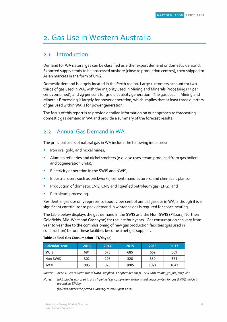
The table below displays the gas demand in the SWIS and the Non-SWIS (Pilbara, Northern
Goldfields, Mid-West and Gascoyne) for the last four years. Gas consumption can vary from
year to year due to the commissioning of new gas production facilities (gas used in
construction) before these facilities become a net gas supplier.
Table 1: Final Gas Consumption - TJ/day (a)
Calendar Year 2013 2014 2015 2016 2017
SWIS 684 678 685 662 669
Non-SWIS 302 296 320 359 374
Total 985 973 1005 1021 1043
Source: AEMO, Gas Bulletin Board Data, supplied (1 September 2017) – “All GBB Points_30_08_2017.xls”
Notes: (a) Excludes gas used in gas shipping (e.g. compressor stations and unaccounted for gas (UFG)) which is around 20 TJ/day.
(b) Data covers the period 1 January to 28 August 2017.
Australian Energy Market Operator Gas Demand Forecasts
9.
Large gas consumers in the SWIS include minerals processing (Alcoa’s Kwinana, Wagerup,
and Pinjarra alumina refineries and BHP’s Kwinana nickel refinery) and electricity generators
(such as Kwinana and Cockburn power stations). Depressed commodity prices for alumina,
mineral sands and nickel have prevented growth in the development of new facilities, which
has kept gas demand static in the SWIS over the last four years.
Non-SWIS consumption is primarily for power generation required by mining projects and
local townships. Around 3,519 MW of gas generation capacity is located at remote mine sites
and in regional centres (such as Halls Creek and Leonora). There is about 444 MW of diesel-
fuelled generation capacity in the Non-SWIS area. Some of this generating capacity may be
converted to gas, particularly if diesel remains more expensive, which would create additional
opportunities for increased gas consumption in the future.
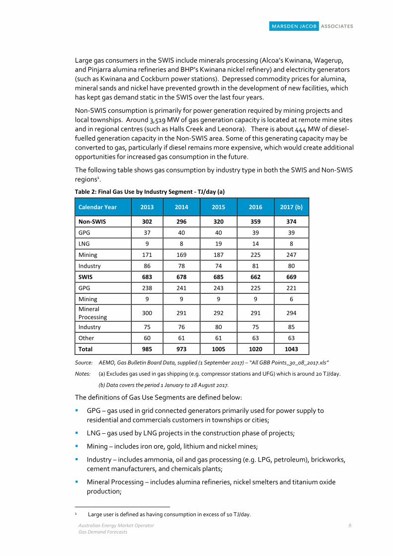
The following table shows gas consumption by industry type in both the SWIS and Non-SWIS
regions1.
Table 2: Final Gas Use by Industry Segment - TJ/day (a)
Calendar Year 2013 2014 2015 2016 2017 (b)
Non-SWIS 302 296 320 359 374
GPG 37 40 40 39 39
LNG 9 8 19 14 8
Mining 171 169 187 225 247
Industry 86 78 74 81 80
SWIS 683 678 685 662 669
GPG 238 241 243 225 221
Mining 9 9 9 9 6
Mineral Processing
300 291 292 291 294
Industry 75 76 80 75 85
Other 60 61 61 63 63
Total 985 973 1005 1020 1043
Source: AEMO, Gas Bulletin Board Data, supplied (1 September 2017) – “All GBB Points_30_08_2017.xls”
Notes: (a) Excludes gas used in gas shipping (e.g. compressor stations and UFG) which is around 20 TJ/day.
(b) Data covers the period 1 January to 28 August 2017.
The definitions of Gas Use Segments are defined below:
GPG – gas used in grid connected generators primarily used for power supply to
residential and commercials customers in townships or cities;
LNG – gas used by LNG projects in the construction phase of projects;
Mining – includes iron ore, gold, lithium and nickel mines;
Industry – includes ammonia, oil and gas processing (e.g. LPG, petroleum), brickworks,
cement manufacturers, and chemicals plants;
Mineral Processing – includes alumina refineries, nickel smelters and titanium oxide
production;
1 Large user is defined as having consumption in excess of 10 TJ/day.
Australian Energy Market Operator Gas Demand Forecasts
10.
Other – residential and business customers on the low-pressure network owned and
operated by ATCO.
2.3 Peak Day Gas Demand
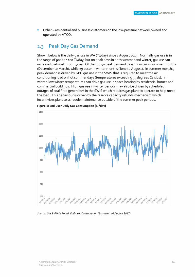
Shown below is the daily gas use in WA (TJ/day) since 1 August 2013. Normally gas use is in the range of 900 to 1100 TJ/day, but on peak days in both summer and winter, gas use can increase to almost 1200 TJ/day. Of the top 40 peak demand days, 11 occur in summer months (December to March), while 29 occur in winter months (June to August). In summer months, peak demand is driven by GPG gas use in the SWIS that is required to meet the air conditioning load on hot summer days (temperatures exceeding 35 degrees Celsius). In winter, low winter temperatures can drive gas use in space heating by residential homes and commercial buildings. High gas use in winter periods may also be driven by scheduled outages of coal fired generators in the SWIS which requires gas plant to operate to help meet the load. This behaviour is driven by the reserve capacity refunds mechanism which incentivises plant to schedule maintenance outside of the summer peak periods.
Figure 1: End User Daily Gas Consumption (TJ/day)
Source: Gas Bulletin Board, End User Consumption (Extracted 10 August 2017)

Australian Energy Market Operator Gas Demand Forecasts
11.
Drivers of Gas Demand in WA
This chapter provides an overview of the key factors that drive gas demand in the state. This
is discussed for each gas use segment in WA (below).
3.1 GPG in the SWIS
Around 2,995 MW of generation capable of using gas (including dual-fuelled gas/diesel), is
currently installed in the SWIS - three-quarters of which is peaking and mid-merit capacity (in
terms of MW, not energy production). Future gas use is based on the relative competitiveness
of coal and gas2, plus the expected entry of large-scale renewable plant in the SWIS to meet
the Commonwealth Government’s Large-scale Renewable Energy Target (LRET). After 2025
it is expected that large-scale renewables will enter the market on economic merit when
existing plants are retired, or demand growth justifies new investment.
Commonwealth commitments to reduce Australia’s greenhouse gas emissions by 26 to 28 per
cent on 2005 levels by 2030, consistent with its COPS213 obligations, could also impact the
generation mix in the Wholesale Electricity Market (WEM). If new policies are developed that
encourage the take-up of low emission generation technologies in the SWIS, such as large-
scale wind and solar plants, then the WEM could have increased intermittent generation and a
lower level of dispatchable generation (e.g. coal or GPG) by 2030.
The potential introduction of Commonwealth Government measures, such as the National
Energy Guarantee (NEG) may help encourage the retention and new investment in
dispatchable generation, such as coal-fired plant and GPG, to help maintain supply reliability
in the WEM.
Major electricity suppliers in the east and west coast of Australia have stated that new coal
generation is not a viable option; the reasons being carbon risk (i.e. re-introduction of a
carbon price) and the declining cost of renewable generation. The higher risk associated with
developing coal fired power stations was noted in the recent report by the Finkel Review to
the Australian government4.
Currently coal generators in the SWIS obtain their coal supplies from the Collie region. Coal is
supplied to the coal power stations at a cost of about $3/GJ. If additional coal were required to
supply a new coal fired power station, in Marsden Jacob’s view there would need to be a
comparable development in coal supply capacity, which would require higher coal prices and
more onerous long term ‘take or pay’ commitments than currently provided to the existing
coal power stations.
2 Black coal from Collie is estimated to cost around $2.84/GJ (2016 dollars).
3 Australia was a signatory to the Paris climate agreement that was negotiated at the 21st Conference of the
Parties (COPS21) of the United Nations Framework Convention on Climate Change in 2017. It was agreed that
emission reductions would be consistent with ensuring that global temperatures increases were well below 2
degrees Celsius above pre-industrial levels and to pursue efforts to limit the temperature increase even further
to 1.5 degrees Celsius.
4 Finkel, A 2017, Independent Review into the Future Security of the National Electricity Market, 21 June 2017, Commonwealth of Australia. Available from: www.environment.gov.au/energy/national-electricity-market-review. [11 September 2017].
Australian Energy Market Operator Gas Demand Forecasts
12.
For the above reasons, Marsden Jacob is of the view that it is unlikely that there will be
significant new investment in large-scale coal powered generation in the SWIS. As a result,
any increase in demand for dispatchable plant in the WEM is likely to be met by GPG.
Even if the NEG provides incentives for coal-fired plant to remain in service, the age of various
units (> 35 years) and the capital and operating costs of keeping them in service may not be
economic. As a result, coal units may still have to retire despite incentives provided by the
NEG.
In summary, GPG gas use in the SWIS is likely to be a function of the following:
Relative competitiveness of different generation technologies (e.g. fuel costs, capital
costs etc.);
Coal plant retirement schedule (would drive GPG gas consumption up);
Renewable investment in response to the LRET and other Commonwealth measures
(potentially reduces GPG gas consumption); and
Given it is unlikely that new coal plant will be built in the WEM, dispatchable demand
growth is likely to be met by new GPG plant (potentially drives GPG gas consumption
upwards).
3.1.1 Relationship between GPG Gas Use and Electricity Demand Forecasts
Future Electricity Demand in the WEM is available from the AEMO5. The forecasts consider
the following factors:
Economic activity (e.g. Gross State Product or GSP);
Population growth;
Weather;
Increased penetration of rooftop photovoltaic (PV) systems;
Deployment of battery storage behind the meter;
Take-up of electricity vehicles;
New block loads (or major projects) entering the SWIS.
The operational consumption forecasts for the SWIS are shown for the high, low and medium
growth cases for the period 2017–18 to 2026–27. Operational consumption is forecast to grow
at a cumulative average growth rate (CAGR) of:
1.7 per cent in the high demand growth scenario.
1.2 per cent in the expected demand growth scenario.
0.7 per cent in the low demand growth scenario.
Graphs of the historical and operational consumption forecasts are shown below.
5 AEMO, 2017 WEM Electricity Statement of Opportunities, June 2017.
Australian Energy Market Operator Gas Demand Forecasts
13.
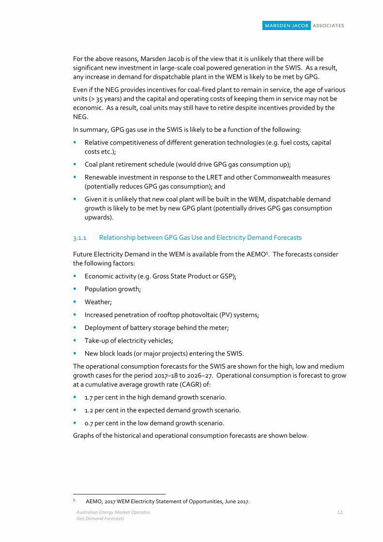
Figure 2: Operational Consumption Forecasts for the WEM
Source: AEMO, 2017 Electricity Statement of Opportunities, For the Wholesale Electricity Market, June 2017
Under the expected scenario, operational consumption in the WEM is forecast to grow from approximately 18,819 GWh in 2017–18 to 20,996 GWh by 2026–27.
The annual growth rates are above the historical trend for the WEM. Operating consumption only grew by 1.09 per cent between 2010-11 and 2015-16. Contributing factors to this lower growth rate include:
Slowing of population growth rates: The long run average is around 2 per cent and the
growth rate for 2013-14, 2014-15 and 2015-16 was 1.7 per cent, 1.3 per cent and 1.0 per
cent, respectively;
Slowing of economic growth which was on average around 4.7 per cent, reduced to only
1.9 per cent in 2015-16.
However, there are further risks to these forecasts. Rapid penetration of rooftop PV by both
residential and commercial customers could further lower operational demand, as could a
longer recovery from the reductions in economic growth experienced in recent years.
The risks of lower growth rates for operating consumption and demand have been
incorporated into Marsden Jacob’s forecasts. This is further discussed in Section 4.3.
3.2 Mining
A significant proportion of gas demand in WA is for onsite power generation to facilitate
mining (e.g. bauxite, iron ore, mineral sands, nickel, lithium etc.).
Once a facility is built, the mine will typically operate at a steady capacity factor to extract the
ore/mineral. If commodity prices increase, existing mines may have some ability to increase
production, but are limited by the capacity of the mine in the short run. If commodity prices
Australian Energy Market Operator Gas Demand Forecasts
14.
fall to low levels, the mine may not be able to recover the cash costs associated with operation
and may close either temporarily or permanently.
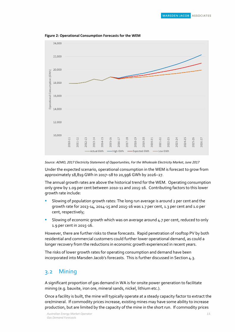
The characteristics of gas use by existing mines is illustrated in the figure below. The figure
shows average gas use by iron ore mines in WA (large gas users only) and the iron ore price
index (real). What this shows is that gas use per mine is not highly correlated with iron prices.
Once constructed, unless a mine is expanded, the mine will typically operate at a constant
level regardless of movements in commodity prices (except if unit prices were to fall below
cash costs of the mine).
Figure 3: Average Gas Demand for Iron Ore Mines in WA
Source: DMP, 2016 Major Commodities Resource File & AEMO Gas Bulletin Board data supplied (1 September 2017) – “All GBB Points_30_08_2017.xls”
Similar relationships exist between output from other mines (e. gold, nickel and bauxite) and
current commodity prices.
The establishment of new mines and facilities is likely to be a function of the trajectory of
future commodity prices (e.g. iron ore and minerals). These prices are in turn a function of
economic activity in Asia, the major destination for our mineral exports. The higher the
forward curve for commodities, the more likely that new mines will be established and
increase gas use in the sector.
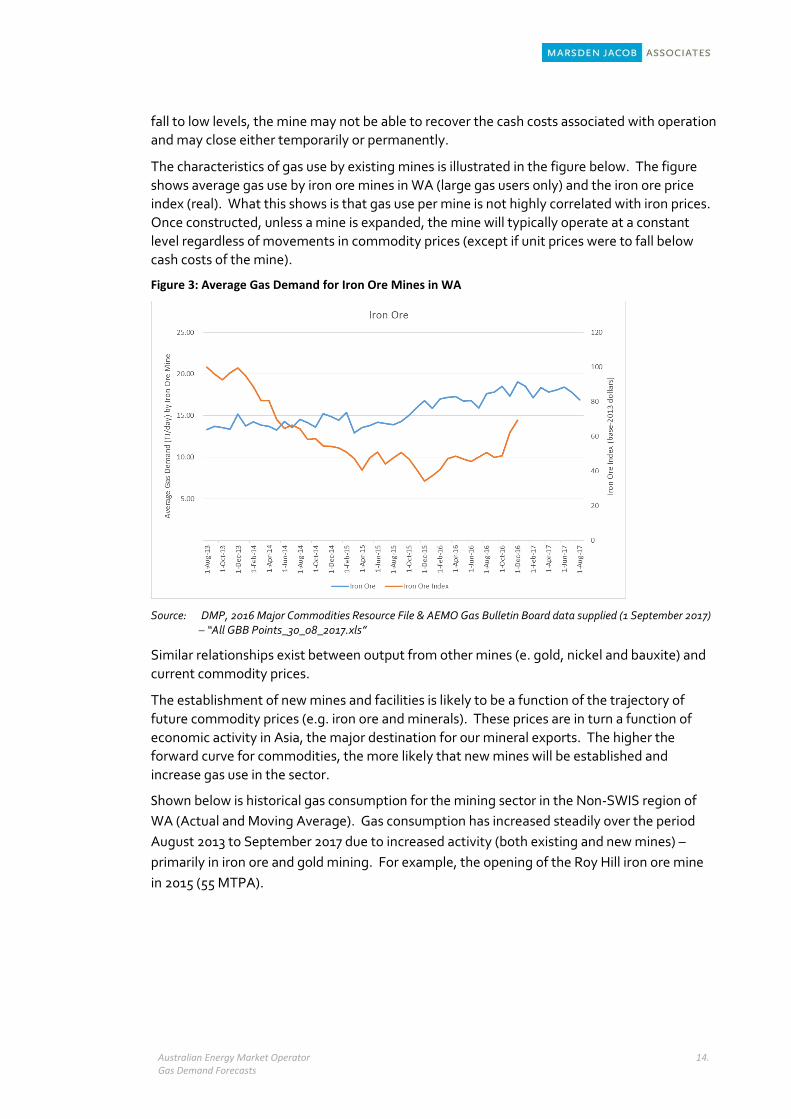
Shown below is historical gas consumption for the mining sector in the Non-SWIS region of
WA (Actual and Moving Average). Gas consumption has increased steadily over the period
August 2013 to September 2017 due to increased activity (both existing and new mines) –
primarily in iron ore and gold mining. For example, the opening of the Roy Hill iron ore mine
in 2015 (55 MTPA).
Australian Energy Market Operator Gas Demand Forecasts
15.
Figure 4: Mining Gas Consumption (Non-SWIS) – TJ/day
Source: AEMO 2017 and Marsden Jacob Analysis 2017
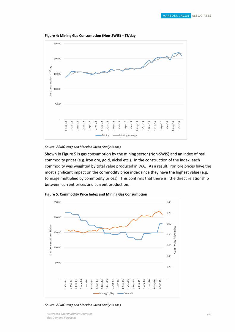
Shown in Figure 5 is gas consumption by the mining sector (Non-SWIS) and an index of real
commodity prices (e.g. iron ore, gold, nickel etc.). In the construction of the index, each
commodity was weighted by total value produced in WA. As a result, iron ore prices have the
most significant impact on the commodity price index since they have the highest value (e.g.
tonnage multiplied by commodity prices). This confirms that there is little direct relationship
between current prices and current production.
Figure 5: Commodity Price Index and Mining Gas Consumption
Source: AEMO 2017 and Marsden Jacob Analysis 2017
Australian Energy Market Operator Gas Demand Forecasts
16.
3.3 Mineral Processing
The mineral processing sector in WA is dominated by alumina production.
Alcoa’s three alumina production facilities in the south west of WA are currently powered
entirely by natural gas, 30 per cent which is used directly in the process and 70 per cent which
goes to power and steam production in three cogeneration plants.
The only other alumina production facility is South32's facility which is powered by a
combination of natural gas and coal. The coal is used in a steam cycle power plant and the gas
is used for direct firing and in a cogeneration plant; the latter produced steam and fed
electricity into the grid. The gas fired cogeneration plant (120 MW) was closed in 2016 due to
a combination of higher gas prices and an excess of baseload generation (both coal and gas
plant) in the SWIS.
Higher gas prices will impact cash margins for existing Alumina operations in WA and could
potentially prevent future developments (e.g. expansion of Alcoa’s Wagerup Facility). If prices
are sufficiently high, these companies will consider coal substitution to meet both power
generation and steam requirements6. Given the depressed commodity process for alumina,
these companies do not have a high tolerance (or willingness to bear) for significantly higher
gas commodity prices.
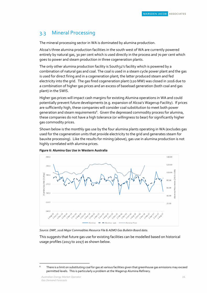
Shown below is the monthly gas use by the four alumina plants operating in WA (excludes gas
used for the cogeneration units that provide electricity to the grid and generates steam for
bauxite processing). Like the results for mining (above), gas use in alumina production is not
highly correlated with alumina prices.
Figure 6: Alumina Gas Use in Western Australia
Source: DMP, 2016 Major Commodities Resource File & AEMO Gas Bulletin Board data.
This suggests that future gas use for existing facilities can be modelled based on historical
usage profiles (2013 to 2017) as shown below.
6 There is a limit on substituting coal for gas at various facilities given that greenhouse gas emissions may exceed
permitted levels. This is particularly a problem at the Wagerup Alumina Refinery.
Australian Energy Market Operator Gas Demand Forecasts
17.
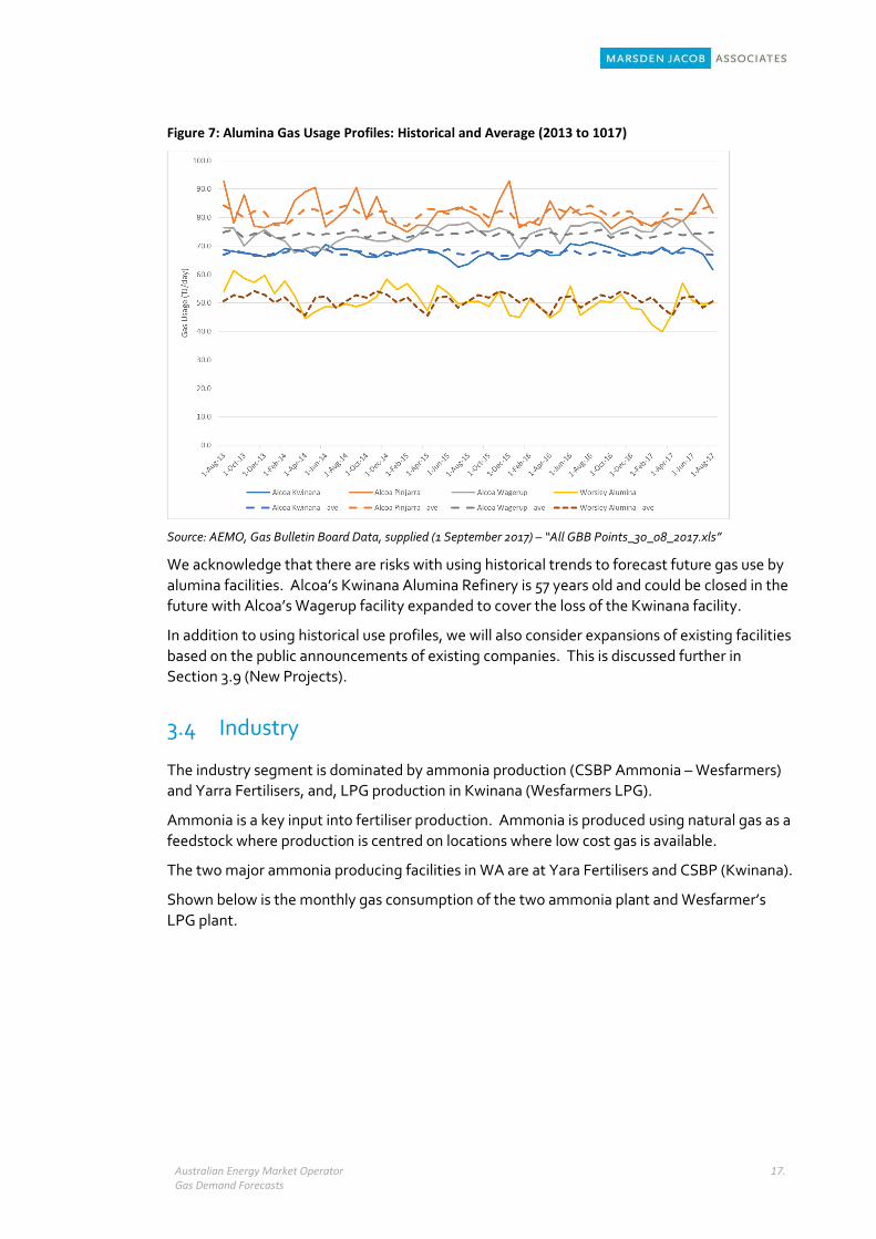
Figure 7: Alumina Gas Usage Profiles: Historical and Average (2013 to 1017)
Source: AEMO, Gas Bulletin Board Data, supplied (1 September 2017) – “All GBB Points_30_08_2017.xls”
We acknowledge that there are risks with using historical trends to forecast future gas use by
alumina facilities. Alcoa’s Kwinana Alumina Refinery is 57 years old and could be closed in the
future with Alcoa’s Wagerup facility expanded to cover the loss of the Kwinana facility.
In addition to using historical use profiles, we will also consider expansions of existing facilities
based on the public announcements of existing companies. This is discussed further in
Section 3.9 (New Projects).
3.4 Industry
The industry segment is dominated by ammonia production (CSBP Ammonia – Wesfarmers)
and Yarra Fertilisers, and, LPG production in Kwinana (Wesfarmers LPG).
Ammonia is a key input into fertiliser production. Ammonia is produced using natural gas as a
feedstock where production is centred on locations where low cost gas is available.
The two major ammonia producing facilities in WA are at Yara Fertilisers and CSBP (Kwinana).
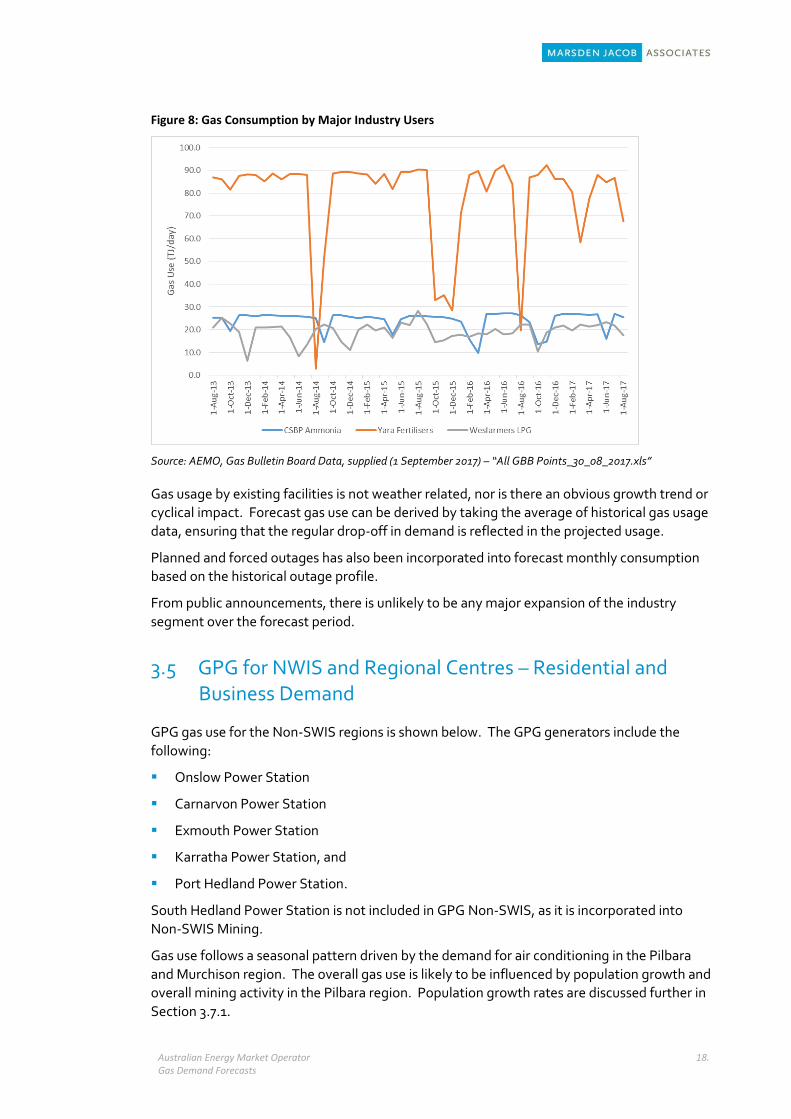
Shown below is the monthly gas consumption of the two ammonia plant and Wesfarmer’s
LPG plant.
Australian Energy Market Operator Gas Demand Forecasts
18.
Figure 8: Gas Consumption by Major Industry Users
Source: AEMO, Gas Bulletin Board Data, supplied (1 September 2017) – “All GBB Points_30_08_2017.xls”
Gas usage by existing facilities is not weather related, nor is there an obvious growth trend or
cyclical impact. Forecast gas use can be derived by taking the average of historical gas usage
data, ensuring that the regular drop-off in demand is reflected in the projected usage.
Planned and forced outages has also been incorporated into forecast monthly consumption
based on the historical outage profile.
From public announcements, there is unlikely to be any major expansion of the industry
segment over the forecast period.
3.5 GPG for NWIS and Regional Centres – Residential and Business Demand
GPG gas use for the Non-SWIS regions is shown below. The GPG generators include the
following:
Onslow Power Station
Carnarvon Power Station
Exmouth Power Station
Karratha Power Station, and
Port Hedland Power Station.
South Hedland Power Station is not included in GPG Non-SWIS, as it is incorporated into
Non-SWIS Mining.
Gas use follows a seasonal pattern driven by the demand for air conditioning in the Pilbara
and Murchison region. The overall gas use is likely to be influenced by population growth and
overall mining activity in the Pilbara region. Population growth rates are discussed further in
Section 3.7.1.
Australian Energy Market Operator Gas Demand Forecasts
19.
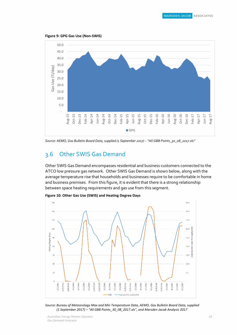
Figure 9: GPG Gas Use (Non-SWIS)
Source: AEMO, Gas Bulletin Board Data, supplied (1 September 2017) – “All GBB Points_30_08_2017.xls”
3.6 Other SWIS Gas Demand
Other SWIS Gas Demand encompasses residential and business customers connected to the
ATCO low pressure gas network. Other SWIS Gas Demand is shown below, along with the
average temperature rise that households and businesses require to be comfortable in home
and business premises. From this figure, it is evident that there is a strong relationship
between space heating requirements and gas use from this segment.
Figure 10: Other Gas Use (SWIS) and Heating Degree Days
Source: Bureau of Meteorology Max and Min Temperature Data, AEMO, Gas Bulletin Board Data, supplied (1 September 2017) – “All GBB Points_30_08_2017.xls”, and Marsden Jacob Analysis 2017
-
5.0
10.0
15.0
20.0
25.0
30.0
35.0
40.0
45.0
50.0
Au
g-1
3
Oct
-13
Dec
-13
Feb
-14
Ap
r-1
4
Jun
-14
Au
g-1
4
Oct
-14
Dec
-14
Feb
-15
Ap
r-1
5
Jun
-15
Au
g-1
5
Oct
-15
Dec
-15
Feb
-16
Ap
r-1
6
Jun
-16
Au
g-1
6
Oct
-16
Dec
-16
Feb
-17
Ap
r-1
7
Jun
-17
Au
g-1
7
Gas
Use
(TJ
/day
)
GPG
Australian Energy Market Operator Gas Demand Forecasts
20.
Drivers of incremental growth for gas demand in non-resource based segments include
population growth (residential consumption) and State Final Demand (SFD): the latter in the
case of large industrial and commercial customers.
Forecasting future growth of gas demand for Other SWIS is complicated by the fact that key
drivers of gas demand (i.e. gas price increases and increased penetration of reverse cycle air
conditioners) have tended to reduce per capita gas demand by both residential and business
customers in the SWIS.
3.7 Drivers of Segment Growth in GPG Non-SWIS and Other SWIS
As outlined above, population, household income, economic growth, gas prices and weather
are factors that can drive gas use in the following segments:
GPG Non-SWIS
Other SWIS (ATCO customers)
3.7.1 Population Growth
Growth in customer numbers has been a key driver of gas consumption in WA. Increasing
residential customer numbers are driven by household formation arising from population
growth.
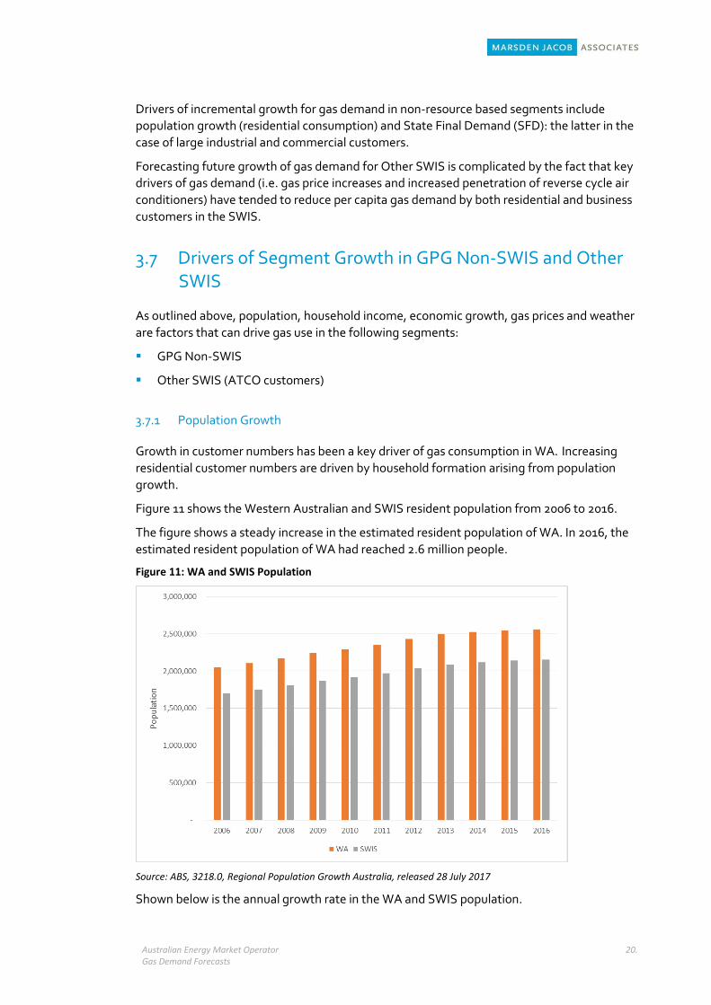
Figure 11 shows the Western Australian and SWIS resident population from 2006 to 2016.
The figure shows a steady increase in the estimated resident population of WA. In 2016, the
estimated resident population of WA had reached 2.6 million people.
Figure 11: WA and SWIS Population
Source: ABS, 3218.0, Regional Population Growth Australia, released 28 July 2017
Shown below is the annual growth rate in the WA and SWIS population.
Australian Energy Market Operator Gas Demand Forecasts
21.
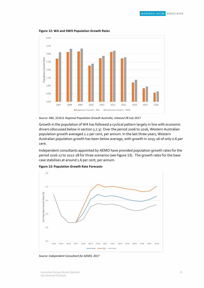
Figure 12: WA and SWIS Population Growth Rates
Source: ABS, 3218.0, Regional Population Growth Australia, released 28 July 2017
Growth in the population of WA has followed a cyclical pattern largely in line with economic
drivers (discussed below in section 3.7.3). Over the period 2006 to 2016, Western Australian
population growth averaged 2.2 per cent, per annum. In the last three years, Western
Australian population growth has been below average, with growth in 2015-16 of only 0.6 per
cent.
Independent consultants appointed by AEMO have provided population growth rates for the
period 2016-17 to 2027-28 for three scenarios (see Figure 13). The growth rates for the base
case stabilises at around 1.6 per cent, per annum.
Figure 13: Population Growth Rate Forecasts
Source: Independent Consultant for AEMO, 2017
Australian Energy Market Operator Gas Demand Forecasts
22.
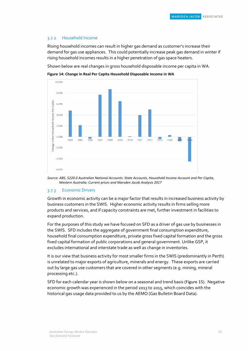
3.7.2 Household Income
Rising household incomes can result in higher gas demand as customer’s increase their
demand for gas use appliances. This could potentially increase peak gas demand in winter if
rising household incomes results in a higher penetration of gas space heaters.
Shown below are real changes in gross household disposable income per capita in WA.
Figure 14: Change in Real Per Capita Household Disposable Income in WA
Source: ABS, 5220.0 Australian National Accounts: State Accounts, Household Income Account and Per Capita, Western Australia: Current prices and Marsden Jacob Analysis 2017
3.7.3 Economic Drivers
Growth in economic activity can be a major factor that results in increased business activity by
business customers in the SWIS. Higher economic activity results in firms selling more
products and services, and if capacity constraints are met, further investment in facilities to
expand production.
For the purposes of this study we have focused on SFD as a driver of gas use by businesses in
the SWIS. SFD includes the aggregate of government final consumption expenditure,
household final consumption expenditure, private gross fixed capital formation and the gross
fixed capital formation of public corporations and general government. Unlike GSP, it
excludes international and interstate trade as well as change in inventories.
It is our view that business activity for most smaller firms in the SWIS (predominantly in Perth)
is unrelated to major exports of agriculture, minerals and energy. These exports are carried
out by large gas use customers that are covered in other segments (e.g. mining, mineral
processing etc.).
SFD for each calendar year is shown below on a seasonal and trend basis (Figure 15). Negative
economic growth was experienced in the period 2013 to 2015, which coincides with the
historical gas usage data provided to us by the AEMO (Gas Bulletin Board Data).

Australian Energy Market Operator Gas Demand Forecasts
23.
Figure 15: State Final Demand - Annual Growth Rates (real)
Source: Compiled by the WA State Treasury. Available from: https://www.treasury.wa.gov.au/Treasury/Economic_Data/State_Final_Demand_(SFD). [8 November 2017].
An independent consultant provided forecasts of SFD for the period 2017 to 2028 by scenario.
It is expected that economic growth will pick up in all scenarios by 2018 and achieve an annual
growth rate of 2.3 per cent per annum.
3.7.4 Retail Gas Prices
Changes in retail gas prices can influence per capita gas consumption. Higher (real) prices can
discourage customers to use gas, while lower prices can encourage gas usage.
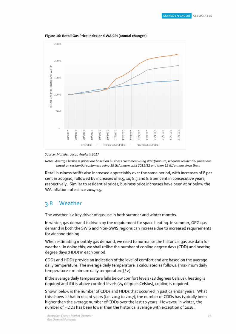
As highlighted below, retail gas prices increased more than the WA Consumer Price Index
(CPI) from 2009/10. Domestic retail gas price rose up to 22 per cent in 2009/10, followed by
increases of 7, 10, 11.6 and 6.4 per cent in consecutive years respectively. However, since
2014/15, retail gas price increases have been at or below the WA inflation rate.
Australian Energy Market Operator Gas Demand Forecasts
24.
Figure 16: Retail Gas Price index and WA CPI (annual changes)
Source: Marsden Jacob Analysis 2017
Notes: Average business prices are based on business customers using 40 GJ/annum, whereas residential prices are based on residential customers using 18 GJ/annum until 2011/12 and then 15 GJ/annum since then.
Retail business tariffs also increased appreciably over the same period, with increases of 8 per
cent in 2009/10, followed by increases of 6.5, 10, 8.3 and 8.6 per cent in consecutive years,
respectively. Similar to residential prices, business price increases have been at or below the
WA inflation rate since 2014-15.
3.8 Weather
The weather is a key driver of gas use in both summer and winter months.
In winter, gas demand is driven by the requirement for space heating. In summer, GPG gas
demand in both the SWIS and Non-SWIS regions can increase due to increased requirements
for air conditioning.
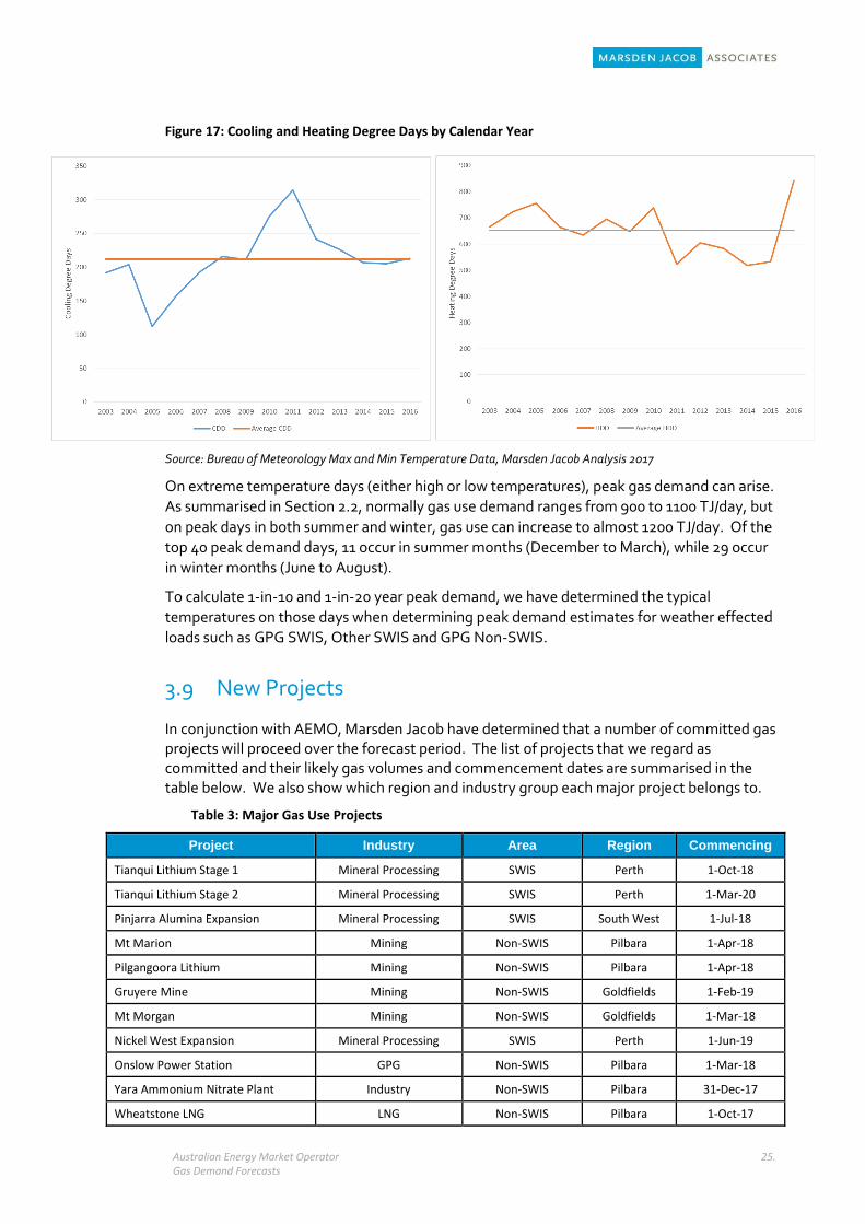
When estimating monthly gas demand, we need to normalise the historical gas use data for weather. In doing this, we shall utilise the number of cooling degree days (CDD) and heating degree days (HDD) in each period.
CDDs and HDDs provide an indication of the level of comfort and are based on the average daily temperature. The average daily temperature is calculated as follows: [maximum daily temperature + minimum daily temperature] / 2].
If the average daily temperature falls below comfort levels (18 degrees Celsius), heating is required and if it is above comfort levels (24 degrees Celsius), cooling is required.
Shown below is the number of CDDs and HDDs that occurred in past calendar years. What this shows is that in recent years (i.e. 2013 to 2017), the number of CDDs has typically been higher than the average number of CDDs over the last 1o years. However, in winter, the number of HDDs has been lower than the historical average with exception of 2016.
Australian Energy Market Operator Gas Demand Forecasts
25.
Figure 17: Cooling and Heating Degree Days by Calendar Year
Source: Bureau of Meteorology Max and Min Temperature Data, Marsden Jacob Analysis 2017
On extreme temperature days (either high or low temperatures), peak gas demand can arise.
As summarised in Section 2.2, normally gas use demand ranges from 900 to 1100 TJ/day, but
on peak days in both summer and winter, gas use can increase to almost 1200 TJ/day. Of the
top 40 peak demand days, 11 occur in summer months (December to March), while 29 occur
in winter months (June to August).
To calculate 1-in-10 and 1-in-20 year peak demand, we have determined the typical
temperatures on those days when determining peak demand estimates for weather effected
loads such as GPG SWIS, Other SWIS and GPG Non-SWIS.
3.9 New Projects
In conjunction with AEMO, Marsden Jacob have determined that a number of committed gas projects will proceed over the forecast period. The list of projects that we regard as committed and their likely gas volumes and commencement dates are summarised in the table below. We also show which region and industry group each major project belongs to.
Table 3: Major Gas Use Projects
Project Industry Area Region Commencing
Tianqui Lithium Stage 1 Mineral Processing SWIS Perth 1-Oct-18
Tianqui Lithium Stage 2 Mineral Processing SWIS Perth 1-Mar-20
Pinjarra Alumina Expansion Mineral Processing SWIS South West 1-Jul-18
Mt Marion Mining Non-SWIS Pilbara 1-Apr-18
Pilgangoora Lithium Mining Non-SWIS Pilbara 1-Apr-18
Gruyere Mine Mining Non-SWIS Goldfields 1-Feb-19
Mt Morgan Mining Non-SWIS Goldfields 1-Mar-18
Nickel West Expansion Mineral Processing SWIS Perth 1-Jun-19
Onslow Power Station GPG Non-SWIS Pilbara 1-Mar-18
Yara Ammonium Nitrate Plant Industry Non-SWIS Pilbara 31-Dec-17
Wheatstone LNG LNG Non-SWIS Pilbara 1-Oct-17

Australian Energy Market Operator Gas Demand Forecasts
26.
Source: Marsden Jacob Analysis 2017
The construction of the Yara Ammonium Nitrate Plant in the Pilbara is unlikely to significantly increase the quantity of gas consumed by Yara Pilbara, but will allow Yara to provide ammonium nitrate to mining, quarrying and construction industries in WA.
In effect, these projects will add around 30 TJ/day to gas demand in the state over the forecast period (excludes gas used in the Wheatstone construction phase which ended in October 2017). These projects have been included in all gas demand scenarios (i.e. Expected, High and Low) over the forecast period.
Australian Energy Market Operator Gas Demand Forecasts
27.
SWIS GPG Gas Use Forecasting Methodology
4.1 Key Drivers
GPG gas use in the SWIS is likely to be a function of the following:
Relative competitiveness of different generation technologies (e.g. fuel costs, capital
costs etc.)
Coal plant retirement schedule;
Renewable investment in response to the LRET and other Commonwealth measures;
Future requirements for dispatchable generation, which includes GPGs;
Demand growth in the SWIS.
4.2 Modelling Approach
GPG demand in the SWIS was calculated using our PROPHET simulation model of the WEM.
The PROPHET simulation model is an electricity market model that can determine market
quantities and prices for each trading interval over multiple years (typically 10 to 20 years).
The model calculates the generation merit order (on an economic basis) of plant in the WEM
on a half-hourly basis, taking into account minimum generation constraints, fuel constraints
and can also incorporate transmission constraints. Requirements to meet the LRET and
emission reduction targets can be incorporated into the model.
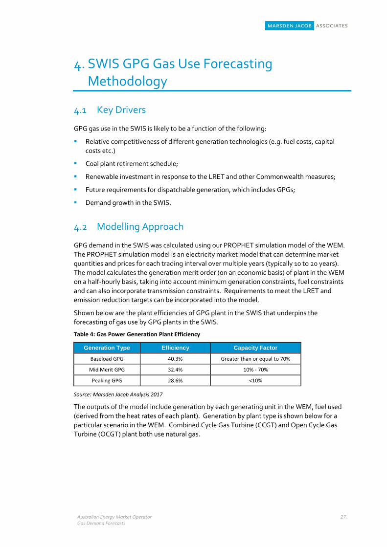
Shown below are the plant efficiencies of GPG plant in the SWIS that underpins the
forecasting of gas use by GPG plants in the SWIS.
Table 4: Gas Power Generation Plant Efficiency
Generation Type Efficiency Capacity Factor
Baseload GPG 40.3% Greater than or equal to 70%
Mid Merit GPG 32.4% 10% - 70%
Peaking GPG 28.6% <10%
Source: Marsden Jacob Analysis 2017
The outputs of the model include generation by each generating unit in the WEM, fuel used
(derived from the heat rates of each plant). Generation by plant type is shown below for a
particular scenario in the WEM. Combined Cycle Gas Turbine (CCGT) and Open Cycle Gas
Turbine (OCGT) plant both use natural gas.
Australian Energy Market Operator Gas Demand Forecasts
28.
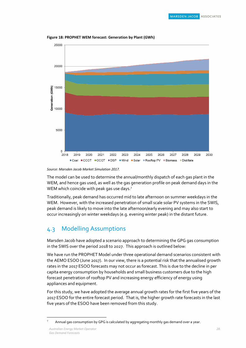
Figure 18: PROPHET WEM forecast: Generation by Plant (GWh)
Source: Marsden Jacob Market Simulation 2017.
The model can be used to determine the annual/monthly dispatch of each gas plant in the
WEM, and hence gas used, as well as the gas generation profile on peak demand days in the
WEM which coincide with peak gas use days.7
Traditionally, peak demand has occurred mid to late afternoon on summer weekdays in the
WEM. However, with the increased penetration of small scale solar PV systems in the SWIS,
peak demand is likely to move into the late afternoon/early evening and may also start to
occur increasingly on winter weekdays (e.g. evening winter peak) in the distant future.
4.3 Modelling Assumptions
Marsden Jacob have adopted a scenario approach to determining the GPG gas consumption
in the SWIS over the period 2018 to 2027. This approach is outlined below:
We have run the PROPHET Model under three operational demand scenarios consistent with
the AEMO ESOO (June 2017). In our view, there is a potential risk that the annualised growth
rates in the 2017 ESOO forecasts may not occur as forecast. This is due to the decline in per
capita energy consumption by households and small business customers due to the high
forecast penetration of rooftop PV and increasing energy efficiency of energy using
appliances and equipment.
For this study, we have adopted the average annual growth rates for the first five years of the
2017 ESOO for the entire forecast period. That is, the higher growth rate forecasts in the last
five years of the ESOO have been removed from this study.
7 Annual gas consumption by GPG is calculated by aggregating monthly gas demand over a year.
Australian Energy Market Operator Gas Demand Forecasts
29.
The annual growth rates in operating consumption for each case is summarised below:
Expected Demand – incorporated expected economic growth and expected rooftop PV
take-up (0.9 per cent/annum).
High Demand – incorporates high economic growth and expected rooftop PV take-up (1.3
per cent/annum).
Low Demand – incorporates low economic growth and expected rooftop PV up-take (0.6
per cent/annum).
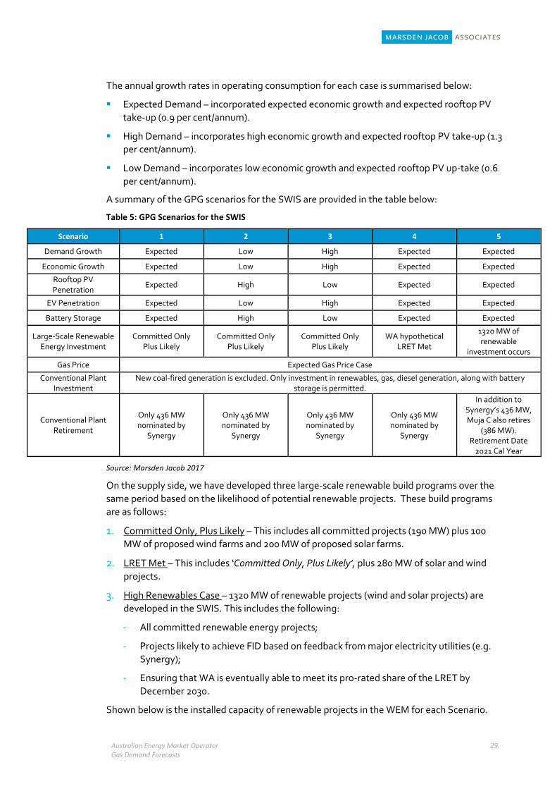
A summary of the GPG scenarios for the SWIS are provided in the table below:
Table 5: GPG Scenarios for the SWIS
Scenario 1 2 3 4 5
Demand Growth Expected Low High Expected Expected
Economic Growth Expected Low High Expected Expected
Rooftop PV Penetration
Expected High Low Expected Expected
EV Penetration Expected Low High Expected Expected
Battery Storage Expected High Low Expected Expected
Large-Scale Renewable Energy Investment
Committed Only Plus Likely
Committed Only Plus Likely
Committed Only Plus Likely
WA hypothetical LRET Met
1320 MW of renewable
investment occurs
Gas Price Expected Gas Price Case
Conventional Plant Investment
New coal-fired generation is excluded. Only investment in renewables, gas, diesel generation, along with battery storage is permitted.
Conventional Plant Retirement
Only 436 MW nominated by
Synergy
Only 436 MW nominated by
Synergy
Only 436 MW nominated by
Synergy
Only 436 MW nominated by
Synergy
In addition to Synergy’s 436 MW, Muja C also retires
(386 MW). Retirement Date
2021 Cal Year
Source: Marsden Jacob 2017
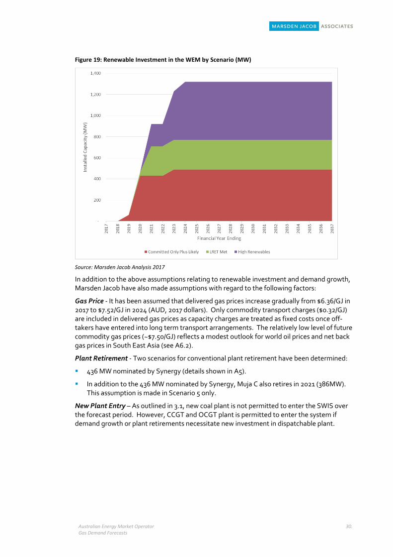
On the supply side, we have developed three large-scale renewable build programs over the
same period based on the likelihood of potential renewable projects. These build programs
are as follows:
1. Committed Only, Plus Likely – This includes all committed projects (190 MW) plus 100
MW of proposed wind farms and 200 MW of proposed solar farms.
2. LRET Met – This includes ‘Committed Only, Plus Likely’, plus 280 MW of solar and wind
projects.
3. High Renewables Case – 1320 MW of renewable projects (wind and solar projects) are
developed in the SWIS. This includes the following:
- All committed renewable energy projects;
- Projects likely to achieve FID based on feedback from major electricity utilities (e.g.
Synergy);
- Ensuring that WA is eventually able to meet its pro-rated share of the LRET by
December 2030.
Shown below is the installed capacity of renewable projects in the WEM for each Scenario.
Australian Energy Market Operator Gas Demand Forecasts
30.
Figure 19: Renewable Investment in the WEM by Scenario (MW)
Source: Marsden Jacob Analysis 2017
In addition to the above assumptions relating to renewable investment and demand growth, Marsden Jacob have also made assumptions with regard to the following factors:
Gas Price - It has been assumed that delivered gas prices increase gradually from $6.36/GJ in 2017 to $7.52/GJ in 2024 (AUD, 2017 dollars). Only commodity transport charges ($0.32/GJ) are included in delivered gas prices as capacity charges are treated as fixed costs once off-takers have entered into long term transport arrangements. The relatively low level of future commodity gas prices (~$7.50/GJ) reflects a modest outlook for world oil prices and net back gas prices in South East Asia (see A6.2).
Plant Retirement - Two scenarios for conventional plant retirement have been determined:
436 MW nominated by Synergy (details shown in A5).
In addition to the 436 MW nominated by Synergy, Muja C also retires in 2021 (386MW). This assumption is made in Scenario 5 only.
New Plant Entry – As outlined in 3.1, new coal plant is not permitted to enter the SWIS over the forecast period. However, CCGT and OCGT plant is permitted to enter the system if demand growth or plant retirements necessitate new investment in dispatchable plant.

Australian Energy Market Operator Gas Demand Forecasts
31.
4.4 Normalised Load Duration Curve (LDC) for Annual and Monthly Load Forecasts
To develop annual and monthly gas consumption, we required annual LDC (17,520 energy demand intervals in a normal year stacked from highest load to lowest).
Figure 20: Load Duration Curve for the SWIS
Source: Public Utilities Office
Although we could have uses past LDCs for this purpose, we need to normalise the historical LDCs for weather as outlined in section 3.8.
In addition to weather adjustments, adjustments were made to the historical LDC to derive the baseline LDC, which requires consideration of:
Population and business growth which drives annual growth in demand; and
Penetration of rooftop PV. Typically, rooftop PV reduces demand in those trading intervals from 10 AM to 4 PM.
4.5 Determining Gas Usage on the Peak Gas Days
A typical load duration curve (discussed above) was used to derive annual and monthly GPG
gas usage (and a 1-in-2 year peak demand forecast). This is not an appropriate approach for
determining the 1-in-10 and 1-in-20 year peak day gas usage given that peak day events are
significantly above average gas usage. Instead, LDCs for extreme peak days were developed,
and the PROPHET model run for those extreme gas use days.
Shown below is the relationship between temperature and gas use by GPGs on high demand
days in the WEM during 2013-2017. Of the top 30 electricity demand days, all have occurred in
summer months since August 2013 (December to March inclusive).
Australian Energy Market Operator Gas Demand Forecasts
32.
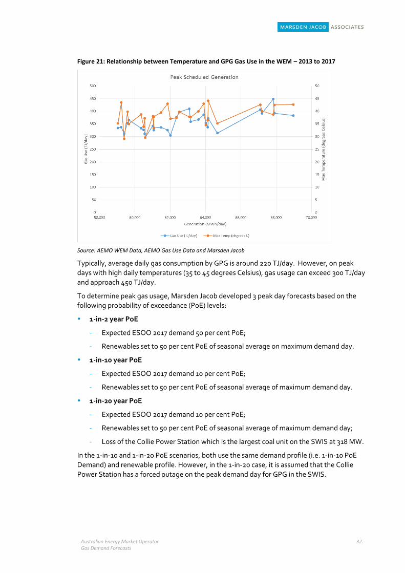
Figure 21: Relationship between Temperature and GPG Gas Use in the WEM – 2013 to 2017
Source: AEMO WEM Data, AEMO Gas Use Data and Marsden Jacob
Typically, average daily gas consumption by GPG is around 220 TJ/day. However, on peak
days with high daily temperatures (35 to 45 degrees Celsius), gas usage can exceed 300 TJ/day
and approach 450 TJ/day.
To determine peak gas usage, Marsden Jacob developed 3 peak day forecasts based on the
following probability of exceedance (PoE) levels:
1-in-2 year PoE
- Expected ESOO 2017 demand 50 per cent PoE;
- Renewables set to 50 per cent PoE of seasonal average on maximum demand day.
1-in-10 year PoE
- Expected ESOO 2017 demand 10 per cent PoE;
- Renewables set to 50 per cent PoE of seasonal average of maximum demand day.
1-in-20 year PoE
- Expected ESOO 2017 demand 10 per cent PoE;
- Renewables set to 50 per cent PoE of seasonal average of maximum demand day;
- Loss of the Collie Power Station which is the largest coal unit on the SWIS at 318 MW.
In the 1-in-10 and 1-in-20 PoE scenarios, both use the same demand profile (i.e. 1-in-10 PoE
Demand) and renewable profile. However, in the 1-in-20 case, it is assumed that the Collie
Power Station has a forced outage on the peak demand day for GPG in the SWIS.
Australian Energy Market Operator Gas Demand Forecasts
33.
Annual and Monthly Demand Forecast Methodology for Gas Use Segments
5.1 Introduction
This chapter outlines the methodology Marsden Jacob utilised to calculate monthly gas
demand for the following gas use segments:
Mining;
Mineral Processing;
Industry;
Non-SWIS GPG;
SWIS Other (ATCO); and
LNG Gas Use.
Our approach to estimating future gas consumption for each segment depended on the
availability and quality of the data available, as well as whether any useful statistical
relationships can be found between gas use and key drivers of gas demand as outlined in
Chapter 3.
5.2 Mineral Processing and Industry Gas Use Segments
For the Mineral Processing and Industry segments, we found no useful statistical relationships
between the monthly gas use data for the period 2013 to 2017 and commodity prices or other
economic drivers (e.g. GSP or SFD). In addition, the data was not weather effected (see
discussion in Section 3.2 to 3.4).
This suggested that a two-pronged approach was needed to forecast gas use by the Mineral
Processing and Industry segments:
Projecting gas use by existing facilities based on historical averages, while, ensuring that the regular drop-off in demand is reflected in the projected usage. Rather than incorporating all gas usage data in developing the average demand for a facility, we use the most recent 12-month period, provided that there is no unusual gas usage patterns due to forced outages or maintenance8; and
Forecast gas use by new facilities that are likely over the forecast period (e.g. committed and FID likely).
We appreciate that there are risks using historical gas demand profiles to forecast future gas consumption, given that there could be efficiency improvements in gas use equipment and machinery overtime.
8 We develop typical outage profiles for each gas use segment.
Australian Energy Market Operator Gas Demand Forecasts
34.
5.3 Mining
As outlined in Section 3.2 of this report, there was not a high correlation between commodity
prices and gas use in WA. To some extent the relationship will be fairly weak since projects
can take many years to develop (2 to 7 years) and prevailing commodity prices in previous
periods (i.e. lagged prices) that drive mining development and ultimately gas consumption if
they have access to pipeline gas.
While we could have attempted to derive relationships between lagged commodity prices and
mining gas demand, there are other factors that drive Mining gas demand in WA. This
includes the resource discovery, costs of developing the mine, access to pipeline gas and
competitiveness of WA mines against competitors in other resource rich nations (e.g. Africa,
North America and South America). Rather than attempting to develop complex
relationships to forecast Mining gas demand in WA, we have undertaken trend analysis and
then overlayed potential capacity constraints to develop CAGR’s for each scenario. The
capacity constraints are based on Marsden Jacob’s view of the amount of non-specific mining
projects that could be developed overtime. This excludes some specific mining projects that
we have modelled separately (discussed in Section 3.9 Major New Gas Use Projects).
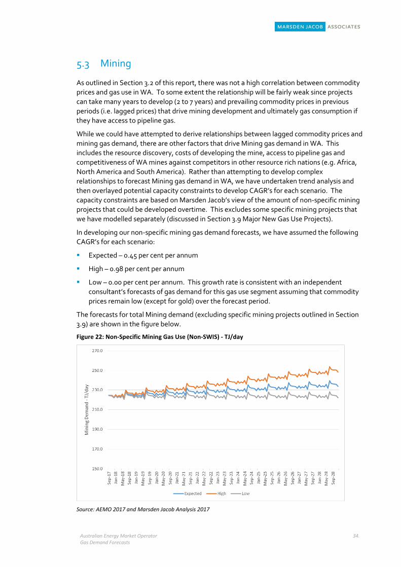
In developing our non-specific mining gas demand forecasts, we have assumed the following
CAGR’s for each scenario:
Expected – 0.45 per cent per annum
High – 0.98 per cent per annum
Low – 0.00 per cent per annum. This growth rate is consistent with an independent
consultant’s forecasts of gas demand for this gas use segment assuming that commodity
prices remain low (except for gold) over the forecast period.
The forecasts for total Mining demand (excluding specific mining projects outlined in Section
3.9) are shown in the figure below.
Figure 22: Non-Specific Mining Gas Use (Non-SWIS) - TJ/day
Source: AEMO 2017 and Marsden Jacob Analysis 2017
Australian Energy Market Operator Gas Demand Forecasts
35.
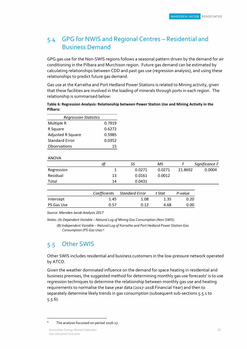
5.4 GPG for NWIS and Regional Centres – Residential and Business Demand
GPG gas use for the Non-SWIS regions follows a seasonal pattern driven by the demand for air
conditioning in the Pilbara and Murchison region. Future gas demand can be estimated by
calculating relationships between CDD and past gas use (regression analysis), and using these
relationships to predict future gas demand.
Gas use at the Karratha and Port Hedland Power Stations is related to Mining activity, given
that these facilities are involved in the loading of minerals through ports in each region. The
relationship is summarised below:
Table 6: Regression Analysis: Relationship between Power Station Use and Mining Activity in the Pilbara:
Source: Marsden Jacob Analysis 2017
Notes: (A) Dependent Variable – Natural Log of Mining Gas Consumption (Non-SWIS)
(B) Independent Variable – Natural Log of Karratha and Port Hedland Power Station Gas Consumption (PS Gas Use).9
5.5 Other SWIS
Other SWIS includes residential and business customers in the low-pressure network operated
by ATCO.
Given the weather dominated influence on the demand for space heating in residential and
business premises, the suggested method for determining monthly gas use forecasts’ is to use
regression techniques to determine the relationship between monthly gas use and heating
requirements to normalise the base year data (2017-2018 Financial Year) and then to
separately determine likely trends in gas consumption (subsequent sub-sections 5.5.1 to
5.5.6).
9 The analysis focussed on period 2016-17.
Regression Statistics
Multiple R 0.7919
R Square 0.6272
Adjusted R Square 0.5985
Standard Error 0.0352
Observations 15
ANOVA
df SS MS F Significance F
Regression 1 0.0271 0.0271 21.8692 0.0004
Residual 13 0.0161 0.0012
Total 14 0.0431
Coefficients Standard Error t Stat P-value
Intercept 1.45 1.08 1.35 0.20
PS Gas Use 0.57 0.12 4.68 0.00
Australian Energy Market Operator Gas Demand Forecasts
36.
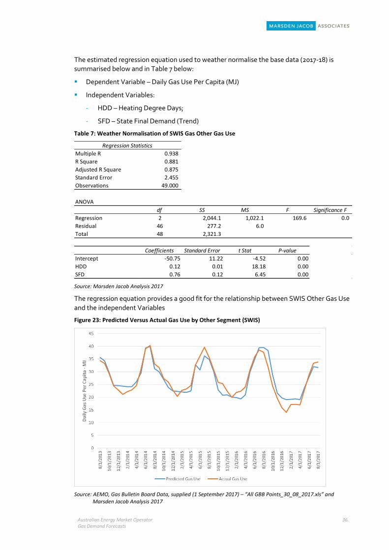
The estimated regression equation used to weather normalise the base data (2017-18) is
summarised below and in Table 7 below:
Dependent Variable – Daily Gas Use Per Capita (MJ)
Independent Variables:
- HDD – Heating Degree Days;
- SFD – State Final Demand (Trend)
Table 7: Weather Normalisation of SWIS Gas Other Gas Use
Source: Marsden Jacob Analysis 2017
The regression equation provides a good fit for the relationship between SWIS Other Gas Use
and the independent Variables
Figure 23: Predicted Versus Actual Gas Use by Other Segment (SWIS)
Source: AEMO, Gas Bulletin Board Data, supplied (1 September 2017) – “All GBB Points_30_08_2017.xls” and Marsden Jacob Analysis 2017
Regression Statistics
Multiple R 0.938
R Square 0.881
Adjusted R Square 0.875
Standard Error 2.455
Observations 49.000
ANOVA
df SS MS F Significance F
Regression 2 2,044.1 1,022.1 169.6 0.0
Residual 46 277.2 6.0
Total 48 2,321.3
Coefficients Standard Error t Stat P-value
Intercept -50.75 11.22 -4.52 0.00
HDD 0.12 0.01 18.18 0.00
SFD 0.76 0.12 6.45 0.00
Australian Energy Market Operator Gas Demand Forecasts
37.
5.5.1 Estimating Trend Growth for “Other SWIS”
Drivers of incremental growth for gas demand for non-resource based segments include
population growth (residential consumption) and SFD: the latter in the case of large industrial
and commercial customers.
Forecasting future growth in gas demand is further complicated by the fact that key drivers of
gas demand (i.e. gas price increases and increased penetration of reverse cycle air
conditioners) tend to reduce per capita gas demand by both residential and business
customers in the SWIS.
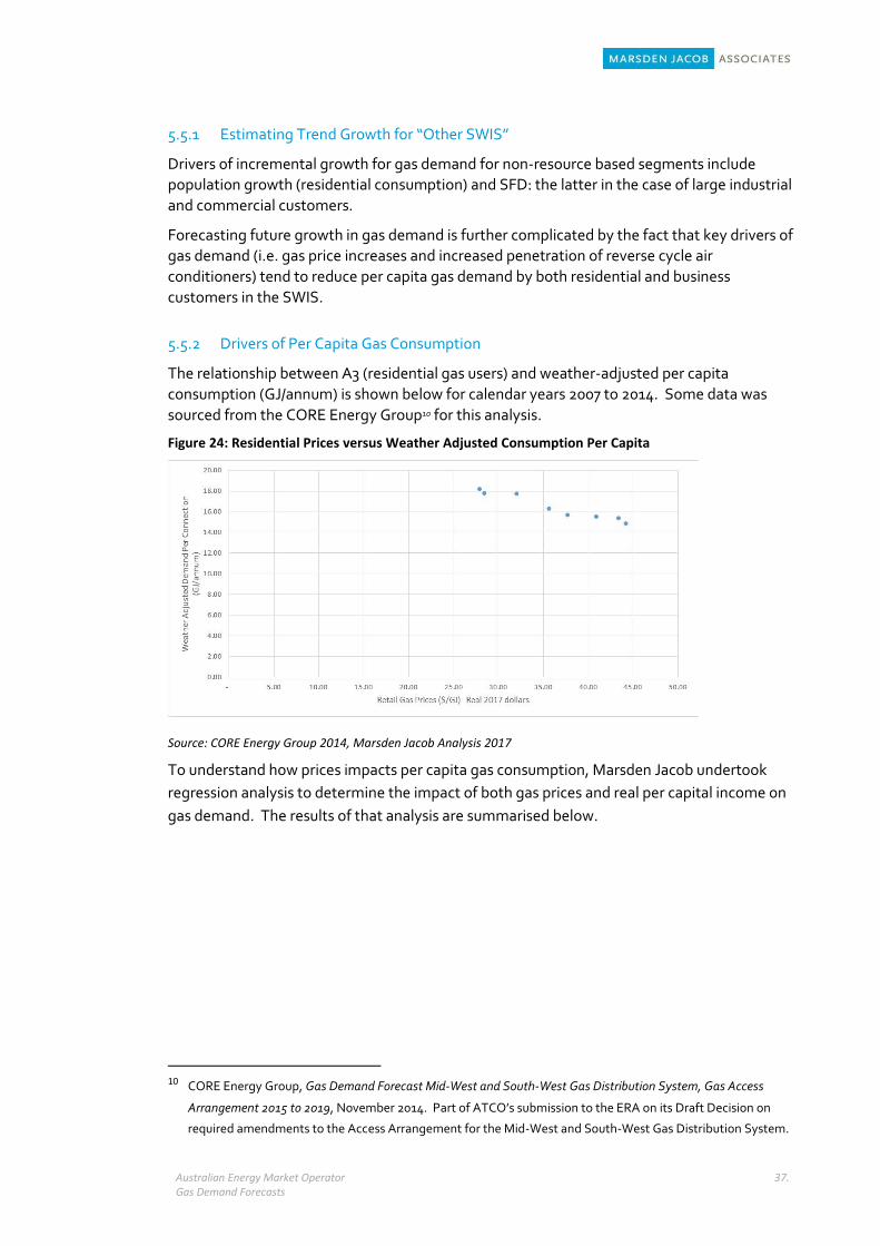
5.5.2 Drivers of Per Capita Gas Consumption
The relationship between A3 (residential gas users) and weather-adjusted per capita
consumption (GJ/annum) is shown below for calendar years 2007 to 2014. Some data was
sourced from the CORE Energy Group10 for this analysis.
Figure 24: Residential Prices versus Weather Adjusted Consumption Per Capita
Source: CORE Energy Group 2014, Marsden Jacob Analysis 2017
To understand how prices impacts per capita gas consumption, Marsden Jacob undertook
regression analysis to determine the impact of both gas prices and real per capital income on
gas demand. The results of that analysis are summarised below.
10 CORE Energy Group, Gas Demand Forecast Mid-West and South-West Gas Distribution System, Gas Access
Arrangement 2015 to 2019, November 2014. Part of ATCO’s submission to the ERA on its Draft Decision on
required amendments to the Access Arrangement for the Mid-West and South-West Gas Distribution System.
Australian Energy Market Operator Gas Demand Forecasts
38.
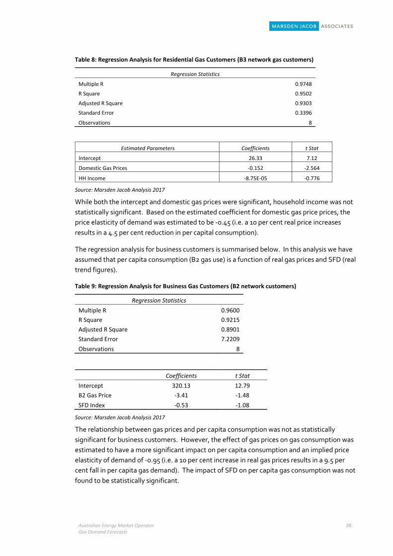
Table 8: Regression Analysis for Residential Gas Customers (B3 network gas customers)
Regression Statistics
Multiple R 0.9748
R Square 0.9502
Adjusted R Square 0.9303
Standard Error 0.3396
Observations 8
Estimated Parameters Coefficients t Stat
Intercept 26.33 7.12
Domestic Gas Prices -0.152 -2.564
HH Income -8.75E-05 -0.776
Source: Marsden Jacob Analysis 2017
While both the intercept and domestic gas prices were significant, household income was not
statistically significant. Based on the estimated coefficient for domestic gas price prices, the
price elasticity of demand was estimated to be -0.45 (i.e. a 10 per cent real price increases
results in a 4.5 per cent reduction in per capital consumption).
The regression analysis for business customers is summarised below. In this analysis we have
assumed that per capita consumption (B2 gas use) is a function of real gas prices and SFD (real
trend figures).
Table 9: Regression Analysis for Business Gas Customers (B2 network customers)
Regression Statistics
Multiple R 0.9600
R Square 0.9215
Adjusted R Square 0.8901
Standard Error 7.2209
Observations 8
Coefficients t Stat
Intercept 320.13 12.79
B2 Gas Price -3.41 -1.48
SFD Index -0.53 -1.08
Source: Marsden Jacob Analysis 2017
The relationship between gas prices and per capita consumption was not as statistically
significant for business customers. However, the effect of gas prices on gas consumption was
estimated to have a more significant impact on per capita consumption and an implied price
elasticity of demand of -0.95 (i.e. a 10 per cent increase in real gas prices results in a 9.5 per
cent fall in per capita gas demand). The impact of SFD on per capita gas consumption was not
found to be statistically significant.
Australian Energy Market Operator Gas Demand Forecasts
39.
While past price increases have reduced per capita gas consumption, it is unlikely that gas
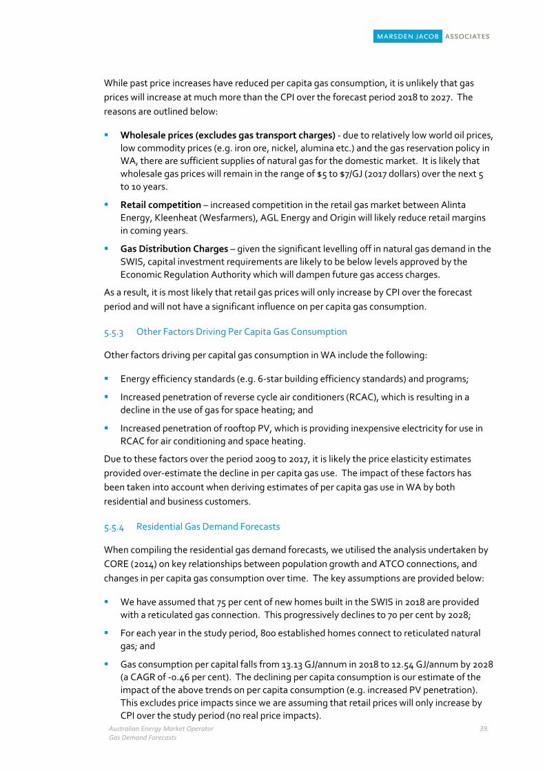
prices will increase at much more than the CPI over the forecast period 2018 to 2027. The
reasons are outlined below:
Wholesale prices (excludes gas transport charges) - due to relatively low world oil prices,
low commodity prices (e.g. iron ore, nickel, alumina etc.) and the gas reservation policy in
WA, there are sufficient supplies of natural gas for the domestic market. It is likely that
wholesale gas prices will remain in the range of $5 to $7/GJ (2017 dollars) over the next 5
to 10 years.
Retail competition – increased competition in the retail gas market between Alinta
Energy, Kleenheat (Wesfarmers), AGL Energy and Origin will likely reduce retail margins
in coming years.
Gas Distribution Charges – given the significant levelling off in natural gas demand in the
SWIS, capital investment requirements are likely to be below levels approved by the
Economic Regulation Authority which will dampen future gas access charges.
As a result, it is most likely that retail gas prices will only increase by CPI over the forecast
period and will not have a significant influence on per capita gas consumption.
5.5.3 Other Factors Driving Per Capita Gas Consumption
Other factors driving per capital gas consumption in WA include the following:
Energy efficiency standards (e.g. 6-star building efficiency standards) and programs;
Increased penetration of reverse cycle air conditioners (RCAC), which is resulting in a
decline in the use of gas for space heating; and
Increased penetration of rooftop PV, which is providing inexpensive electricity for use in
RCAC for air conditioning and space heating.
Due to these factors over the period 2009 to 2017, it is likely the price elasticity estimates
provided over-estimate the decline in per capita gas use. The impact of these factors has
been taken into account when deriving estimates of per capita gas use in WA by both
residential and business customers.
5.5.4 Residential Gas Demand Forecasts
When compiling the residential gas demand forecasts, we utilised the analysis undertaken by
CORE (2014) on key relationships between population growth and ATCO connections, and
changes in per capita gas consumption over time. The key assumptions are provided below:
We have assumed that 75 per cent of new homes built in the SWIS in 2018 are provided
with a reticulated gas connection. This progressively declines to 70 per cent by 2028;
For each year in the study period, 800 established homes connect to reticulated natural
gas; and
Gas consumption per capital falls from 13.13 GJ/annum in 2018 to 12.54 GJ/annum by 2028
(a CAGR of -0.46 per cent). The declining per capita consumption is our estimate of the
impact of the above trends on per capita consumption (e.g. increased PV penetration).
This excludes price impacts since we are assuming that retail prices will only increase by
CPI over the study period (no real price impacts).
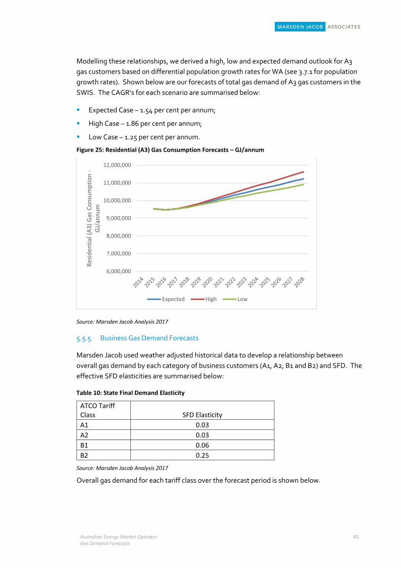
Australian Energy Market Operator Gas Demand Forecasts
40.
Modelling these relationships, we derived a high, low and expected demand outlook for A3
gas customers based on differential population growth rates for WA (see 3.7.1 for population
growth rates). Shown below are our forecasts of total gas demand of A3 gas customers in the
SWIS. The CAGR’s for each scenario are summarised below:
Expected Case – 1.54 per cent per annum;
High Case – 1.86 per cent per annum;
Low Case – 1.25 per cent per annum.
Figure 25: Residential (A3) Gas Consumption Forecasts – GJ/annum
Source: Marsden Jacob Analysis 2017
5.5.5 Business Gas Demand Forecasts
Marsden Jacob used weather adjusted historical data to develop a relationship between
overall gas demand by each category of business customers (A1, A2, B1 and B2) and SFD. The
effective SFD elasticities are summarised below:
Table 10: State Final Demand Elasticity
ATCO Tariff Class SFD Elasticity
A1 0.03
A2 0.03
B1 0.06
B2 0.25
Source: Marsden Jacob Analysis 2017
Overall gas demand for each tariff class over the forecast period is shown below.
6,000,000
7,000,000
8,000,000
9,000,000
10,000,000
11,000,000
12,000,000
Res
iden
tial
(A
3)
Gas
Co
nsu
mp
tio
n -
GJ/
ann
um
Expected High Low
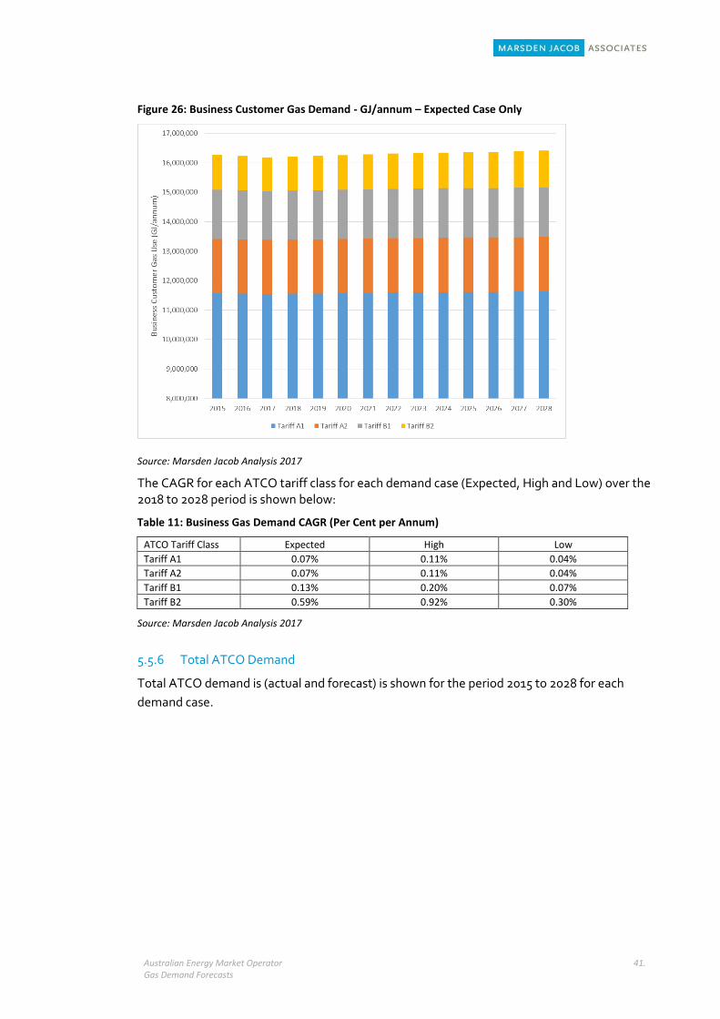
Australian Energy Market Operator Gas Demand Forecasts
41.
Figure 26: Business Customer Gas Demand - GJ/annum – Expected Case Only
Source: Marsden Jacob Analysis 2017
The CAGR for each ATCO tariff class for each demand case (Expected, High and Low) over the 2018 to 2028 period is shown below:
Table 11: Business Gas Demand CAGR (Per Cent per Annum)
ATCO Tariff Class Expected High Low
Tariff A1 0.07% 0.11% 0.04%
Tariff A2 0.07% 0.11% 0.04%
Tariff B1 0.13% 0.20% 0.07%
Tariff B2 0.59% 0.92% 0.30%
Source: Marsden Jacob Analysis 2017
5.5.6 Total ATCO Demand
Total ATCO demand is (actual and forecast) is shown for the period 2015 to 2028 for each
demand case.
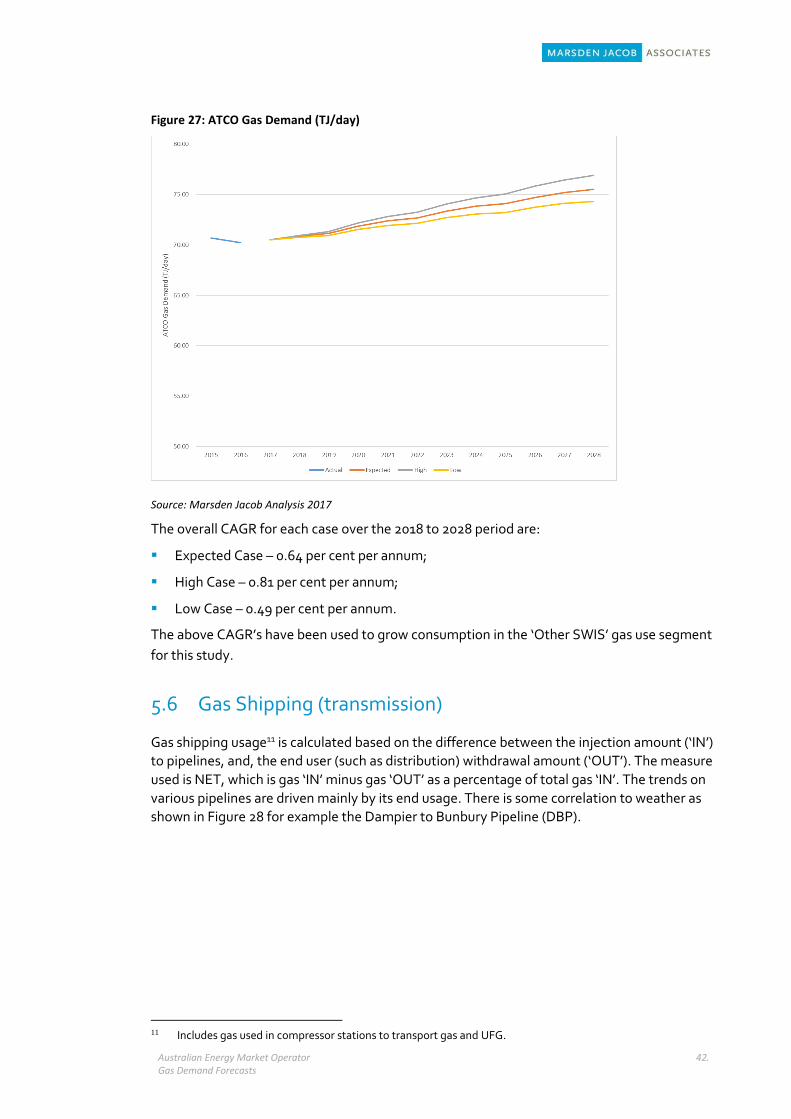
Australian Energy Market Operator Gas Demand Forecasts
42.
Figure 27: ATCO Gas Demand (TJ/day)
Source: Marsden Jacob Analysis 2017
The overall CAGR for each case over the 2018 to 2028 period are:
Expected Case – 0.64 per cent per annum;
High Case – 0.81 per cent per annum;
Low Case – 0.49 per cent per annum.
The above CAGR’s have been used to grow consumption in the ‘Other SWIS’ gas use segment
for this study.
5.6 Gas Shipping (transmission)
Gas shipping usage11 is calculated based on the difference between the injection amount (‘IN’)
to pipelines, and, the end user (such as distribution) withdrawal amount (‘OUT’). The measure
used is NET, which is gas ‘IN’ minus gas ‘OUT’ as a percentage of total gas ‘IN’. The trends on
various pipelines are driven mainly by its end usage. There is some correlation to weather as
shown in Figure 28 for example the Dampier to Bunbury Pipeline (DBP).
11 Includes gas used in compressor stations to transport gas and UFG.
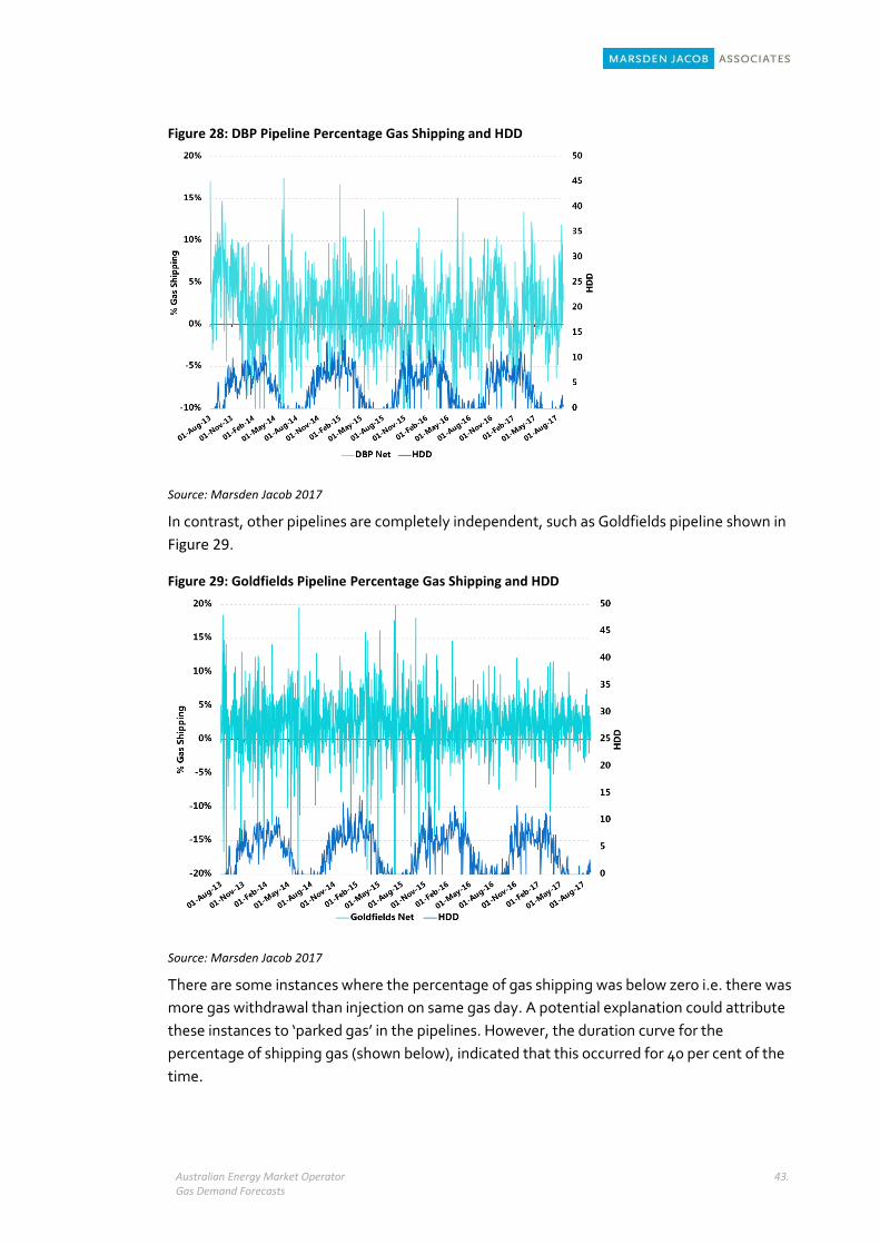
Australian Energy Market Operator Gas Demand Forecasts
43.
Figure 28: DBP Pipeline Percentage Gas Shipping and HDD
Source: Marsden Jacob 2017
In contrast, other pipelines are completely independent, such as Goldfields pipeline shown in
Figure 29.
Figure 29: Goldfields Pipeline Percentage Gas Shipping and HDD
Source: Marsden Jacob 2017
There are some instances where the percentage of gas shipping was below zero i.e. there was
more gas withdrawal than injection on same gas day. A potential explanation could attribute
these instances to ‘parked gas’ in the pipelines. However, the duration curve for the
percentage of shipping gas (shown below), indicated that this occurred for 40 per cent of the
time.
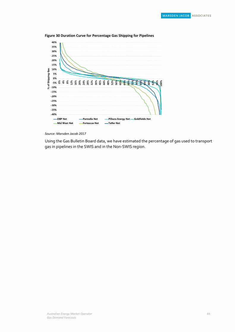
Australian Energy Market Operator Gas Demand Forecasts
44.
Figure 30 Duration Curve for Percentage Gas Shipping for Pipelines
Source: Marsden Jacob 2017
Using the Gas Bulletin Board data, we have estimated the percentage of gas used to transport
gas in pipelines in the SWIS and in the Non-SWIS region.
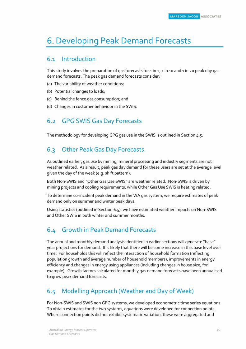
Australian Energy Market Operator Gas Demand Forecasts
45.
Developing Peak Demand Forecasts
6.1 Introduction
This study involves the preparation of gas forecasts for 1 in 2, 1 in 10 and 1 in 20 peak day gas demand forecasts. The peak gas demand forecasts consider:
(a) The variability of weather conditions;
(b) Potential changes to loads;
(c) Behind the fence gas consumption; and
(d) Changes in customer behaviour in the SWIS.
6.2 GPG SWIS Gas Day Forecasts
The methodology for developing GPG gas use in the SWIS is outlined in Section 4.5.
6.3 Other Peak Gas Day Forecasts.
As outlined earlier, gas use by mining, mineral processing and industry segments are not
weather related. As a result, peak gas day demand for these users are set at the average level
given the day of the week (e.g. shift pattern).
Both Non-SWIS and “Other Gas Use SWIS” are weather related. Non-SWIS is driven by
mining projects and cooling requirements, while Other Gas Use SWIS is heating related.
To determine co-incident peak demand in the WA gas system, we require estimates of peak
demand only on summer and winter peak days.
Using statistics (outlined in Section 6.5), we have estimated weather impacts on Non-SWIS
and Other SWIS in both winter and summer months.
6.4 Growth in Peak Demand Forecasts
The annual and monthly demand analysis identified in earlier sections will generate “base”
year projections for demand. It is likely that there will be some increase in this base level over
time. For households this will reflect the interaction of household formation (reflecting
population growth and average number of household members), improvements in energy
efficiency and changes in energy using appliances (including changes in house size, for
example). Growth factors calculated for monthly gas demand forecasts have been annualised
to grow peak demand forecasts.
6.5 Modelling Approach (Weather and Day of Week)
For Non-SWIS and SWIS non GPG systems, we developed econometric time series equations.
To obtain estimates for the two systems, equations were developed for connection points.
Where connection points did not exhibit systematic variation, these were aggregated and
Australian Energy Market Operator Gas Demand Forecasts
46.
modelled to obtain estimates of volatility. The existing data for each were detrended to
identify within year variations.
The effect of weather will be modelled primarily through temperature data measured at the
nearest Bureau of Meteorology site that includes a significant history (e.g. Perth or Port
Hedland Airports). The effect of weather is incorporated using CDD and HDD days. Analysis
in the eastern states suggests that the responsiveness of demand to these hot and cold days is
influenced by time of year. To simulate the time of year impacts on gas demand, we tested a
cosine function to capture these seasonal impacts. This means that an extreme CDD
occurring in summer can have a different impact to one with the same value occurring in
spring. Our analysis (shown in Table 12 and 13) found that the cosine specification of the
demand equation was a good fit and was used in the development of peak demand forecasts
for “Other SWIS” and “Non-SWIS”.
In addition, demand models were tested for Public Holidays, weekends, day of week effects
(particularly Friday), school holidays and separate estimations for Christmas / New Year
holidays.
Specifications that included solely independent variables saw significant serial correlation. All
models were then estimated using an autoregressive 1 (AR1) process for residuals which
significantly improved the strength of the relationship.
In the case of Other SWIS, one function was derived that tested for all of the above-
mentioned elements (e.g. serial correlation). In the case of Non-SWIS, separate functions
were estimated for each of Carnarvon, Esperance, Exmouth, Hill 60, Karratha, Yurrali Maya,
Yara fertilizers and “other”.
Table 12: Other SWIS function
Variable Co-efficient
Constant 417.31
Perth_CDD -1.014
Perth_HDD 2.000
Cosine 10.04
Saturday -2.86
AR (1) 0.85
S.E. of regression 11.30
Source: Marsden Jacob Analysis 2017
Table 13: Non-SWIS Co-Efficients
Carnarvon Power Station
Exmouth Power Station
Hill 60 Power Station
Karratha Power Station
Yurrali Maya Power Station
Yara fertilizers Other
Constant 1.321 0.702 0.104 11.884 26.023 78.054 254.417
CDD
HDD 0.008 0.039 0.149 0.099 School_ holidays
0.054
Sunday -0.065 -0.053 -0.008 0.173 0.888
Saturday -0.072 -0.007 0.817
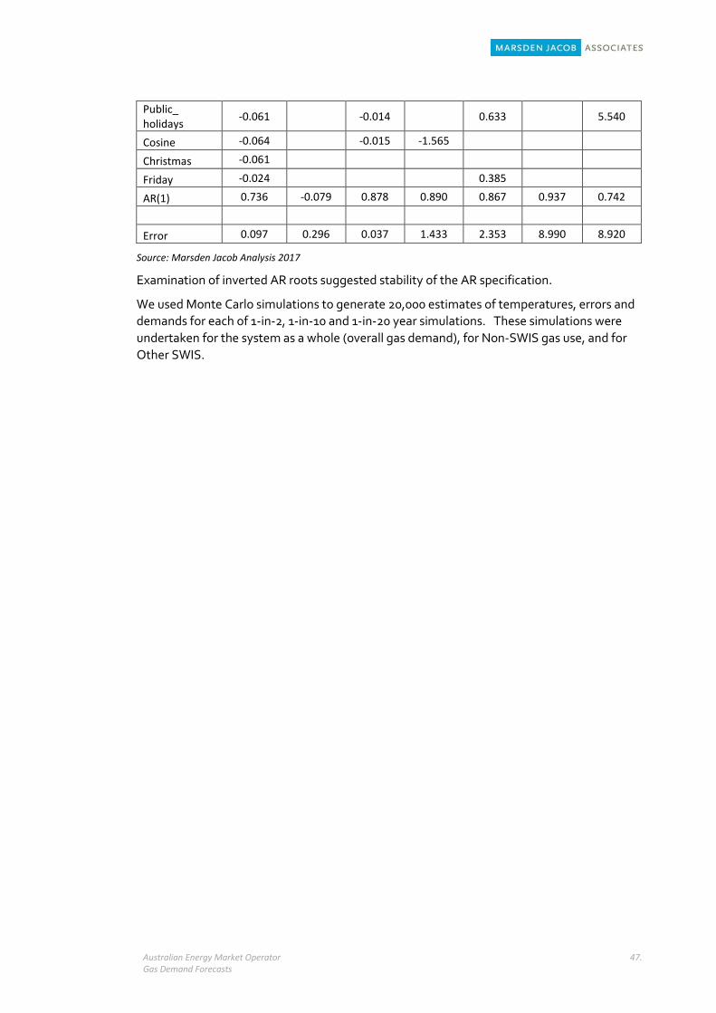
Australian Energy Market Operator Gas Demand Forecasts
47.
Public_ holidays
-0.061
-0.014
0.633
5.540
Cosine -0.064 -0.015 -1.565
Christmas -0.061
Friday -0.024 0.385
AR(1) 0.736 -0.079 0.878 0.890 0.867 0.937 0.742
Error 0.097 0.296 0.037 1.433 2.353 8.990 8.920
Source: Marsden Jacob Analysis 2017
Examination of inverted AR roots suggested stability of the AR specification.
We used Monte Carlo simulations to generate 20,000 estimates of temperatures, errors and
demands for each of 1-in-2, 1-in-10 and 1-in-20 year simulations. These simulations were
undertaken for the system as a whole (overall gas demand), for Non-SWIS gas use, and for
Other SWIS.
Australian Energy Market Operator Gas Demand Forecasts
48.
Annual Average Gas Demand Forecasts
In this section we present the final energy consumption forecasts generated after applying the
methodology described in the previous sections of this report.
7.1 Gas Use Scenarios
Five scenarios were developed for determining annual and monthly gas demand forecasts.
These scenarios were also used in the development of peak demand forecasts summarised in
Chapter 8. These scenarios are summarised below:
Expected Case – future growth is based on expected growth in the following key drivers:
population, economic growth, mining outlook, electricity demand in the SWIS and only
committed large-scale renewable projects proceeding in the SWIS.
High Case - future growth is based on high growth in the following key drivers:
population, economic growth, mining outlook and electricity demand in the SWIS. Only
committed large-scale renewable projects are assumed to proceed in the SWIS.
Low Case - future growth is based on low growth in the following key drivers: population,
economic growth, mining outlook and electricity demand in the SWIS. Only committed
and highly likely large-scale renewable projects are assumed to proceed in the SWIS (490
MW).
Expected Case plus LRET Met - future growth is based on expected growth in the
following key drivers: population, economic growth, mining outlook and electricity
demand in the SWIS. Both committed and likely large-scale renewable projects (490 MW)
and some additional large-scale wind and solar projects (280 MW) are assumed to
proceed in the SWIS which results in the pro-rated LRET for WA being exceeded (3600
GWh of renewable generation versus a pro-rated LRET target of 3267 GWh).
Expected Case plus High Renewables - future growth is based on expected growth in the
following key drivers: population, economic growth, mining outlook and electricity
demand in the SWIS. It is assumed that 1320 MW of renewable projects (only wind and
solar projects) are developed in the SWIS and that the Muja C coal-fired power station
(436 MW nameplate capacity) retires in 2026.
7.2 Average Daily Gas Demand Forecasts
The annual daily final gas demand forecasts for WA in the Expected Case (TJ/day) is shown
below for each calendar year of the forecast period (calculated by summing monthly demand
forecasts). We have also calculated monthly gas demand and demand by financial year (not
shown here).
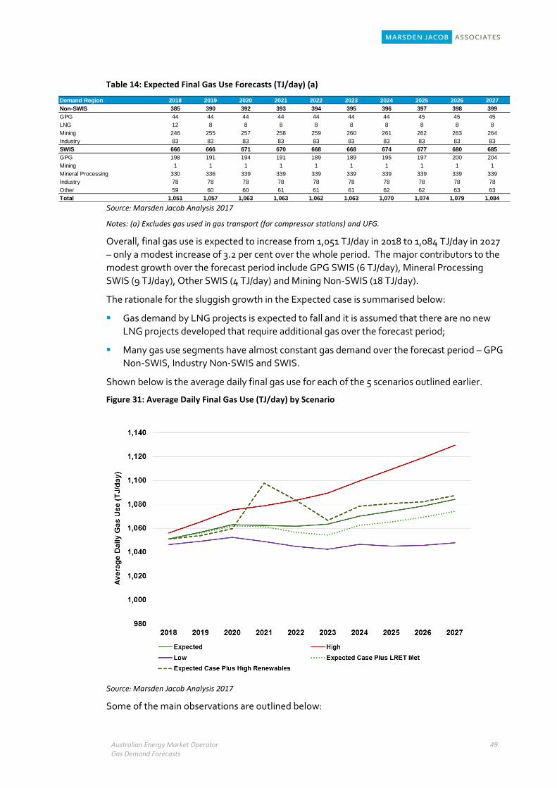
Australian Energy Market Operator Gas Demand Forecasts
49.
Table 14: Expected Final Gas Use Forecasts (TJ/day) (a)
Source: Marsden Jacob Analysis 2017
Notes: (a) Excludes gas used in gas transport (for compressor stations) and UFG.
Overall, final gas use is expected to increase from 1,051 TJ/day in 2018 to 1,084 TJ/day in 2027
– only a modest increase of 3.2 per cent over the whole period. The major contributors to the
modest growth over the forecast period include GPG SWIS (6 TJ/day), Mineral Processing
SWIS (9 TJ/day), Other SWIS (4 TJ/day) and Mining Non-SWIS (18 TJ/day).
The rationale for the sluggish growth in the Expected case is summarised below:
Gas demand by LNG projects is expected to fall and it is assumed that there are no new
LNG projects developed that require additional gas over the forecast period;
Many gas use segments have almost constant gas demand over the forecast period – GPG
Non-SWIS, Industry Non-SWIS and SWIS.
Shown below is the average daily final gas use for each of the 5 scenarios outlined earlier.
Figure 31: Average Daily Final Gas Use (TJ/day) by Scenario
Source: Marsden Jacob Analysis 2017
Some of the main observations are outlined below:
Demand Region 2018 2019 2020 2021 2022 2023 2024 2025 2026 2027
Non-SWIS 385 390 392 393 394 395 396 397 398 399
GPG 44 44 44 44 44 44 44 45 45 45
LNG 12 8 8 8 8 8 8 8 8 8
Mining 246 255 257 258 259 260 261 262 263 264
Industry 83 83 83 83 83 83 83 83 83 83
SWIS 666 666 671 670 668 668 674 677 680 685
GPG 198 191 194 191 189 189 195 197 200 204
Mining 1 1 1 1 1 1 1 1 1 1
Mineral Processing 330 336 339 339 339 339 339 339 339 339
Industry 78 78 78 78 78 78 78 78 78 78
Other 59 60 60 61 61 61 62 62 63 63
Total 1,051 1,057 1,063 1,063 1,062 1,063 1,070 1,074 1,079 1,084
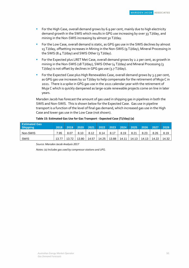
Australian Energy Market Operator Gas Demand Forecasts
50.
For the High Case, overall demand grows by 6.9 per cent, mainly due to high electricity
demand growth in the SWIS which results in GPG use increasing by over 33 TJ/day, and
mining in the Non-SWIS increasing by almost 30 TJ/day.
For the Low Case, overall demand is static, as GPG gas use in the SWIS declines by almost
15 TJ/day, offsetting increases in Mining in the Non-SWIS (9 TJ/day), Mineral Processing in
the SWIS (8.4 TJ/day) and SWIS Other (3 TJ/day).
For the Expected plus LRET Met Case, overall demand grows by 2.2 per cent, as growth in
mining in the Non-SWIS (18 TJ/day), SWIS Other (4 TJ/day) and Mineral Processing (3
TJ/day) is not offset by declines in GPG gas use (3.7 TJ/day).
For the Expected Case plus High Renewables Case, overall demand grows by 3.5 per cent,
as GPG gas use increases by 10 TJ/day to help compensate for the retirement of Muja C in
2021. There is a spike in GPG gas use in the 2021 calendar year with the retirement of
Muja C which is quickly dampened as large-scale renewable projects come on line in later
years.
Marsden Jacob has forecast the amount of gas used in shipping gas in pipelines in both the
SWIS and Non-SWIS. This is shown below for the Expected Case. Gas use in pipeline
transport is a function of the level of final gas demand, which increased gas use in the High
Case and lower gas use in the Low Case (not shown).
Table 15: Estimated Gas Use for Gas Transport - Expected Case (TJ/day) (a)
Estimated Gas Shipping 2018 2019 2020 2021 2022 2023 2024 2025 2026 2027 2028
Non-SWIS 7.95 8.07 8.10 8.12 8.14 8.17 8.19 8.21 8.23 8.26 8.19
SWIS 13.77 13.72 13.80 14.57 14.25 13.88 14.11 14.13 14.13 14.22 14.32
Source: Marsden Jacob Analysis 2017
Notes: (a) Includes gas used by compressor stations and UFG.
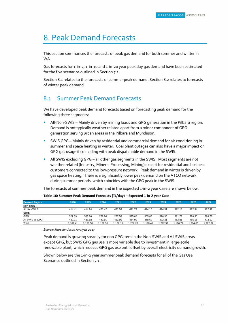
Australian Energy Market Operator Gas Demand Forecasts
51.
Peak Demand Forecasts
This section summarises the forecasts of peak gas demand for both summer and winter in
WA.
Gas forecasts for 1-in-2, 1-in-10 and 1-in-20 year peak day gas demand have been estimated
for the five scenarios outlined in Section 7.1.
Section 8.1 relates to the forecasts of summer peak demand. Section 8.2 relates to forecasts
of winter peak demand.
8.1 Summer Peak Demand Forecasts
We have developed peak demand forecasts based on forecasting peak demand for the
following three segments:
All-Non-SWIS – Mainly driven by mining loads and GPG generation in the Pilbara region.
Demand is not typically weather related apart from a minor component of GPG
generation serving urban areas in the Pilbara and Murchison.
SWIS GPG – Mainly driven by residential and commercial demand for air conditioning in
summer and space heating in winter. Coal plant outages can also have a major impact on
GPG gas usage if coinciding with peak dispatchable demand in the SWIS.
All SWIS excluding GPG – all other gas segments in the SWIS. Most segments are not
weather related (Industry, Mineral Processing, Mining) except for residential and business
customers connected to the low-pressure network. Peak demand in winter is driven by
gas space heating. There is a significantly lower peak demand on the ATCO network
during summer periods, which coincides with the GPG peak in the SWIS.
The forecasts of summer peak demand in the Expected 1-in-2 year Case are shown below.
Table 16: Summer Peak Demand Forecasts (TJ/day) – Expected 1-in-2 year Case
Source: Marsden Jacob Analysis 2017
Peak demand is growing steadily for non GPG item in the Non-SWIS and All SWIS areas
except GPG, but SWIS GPG gas use is more variable due to investment in large-scale
renewable plant, which reduces GPG gas use until offset by overall electricity demand growth.
Shown below are the 1-in-2 year summer peak demand forecasts for all of the Gas Use
Scenarios outlined in Section 7.1.
Demand Region 2018 2019 2020 2021 2022 2023 2024 2025 2026 2027
Non-SWIS
All Non-SWIS 414.41 414.24 421.42 421.58 421.73 424.16 424.31 422.18 422.34 422.92
SWIS
GPG 327.69 303.66 279.96 287.58 325.65 305.65 316.30 311.73 326.36 326.78
All SWIS ex GPG 439.31 438.68 449.91 453.00 454.90 468.60 472.31 462.81 466.15 473.12
Total 1,181.41 1,156.58 1,151.30 1,162.16 1,202.28 1,198.41 1,212.92 1,196.72 1,214.85 1,222.82
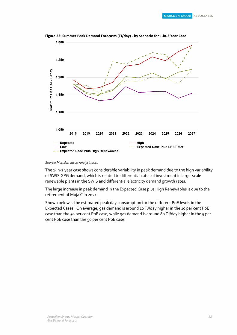
Australian Energy Market Operator Gas Demand Forecasts
52.
Figure 32: Summer Peak Demand Forecasts (TJ/day) - by Scenario for 1-in-2 Year Case
Source: Marsden Jacob Analysis 2017
The 1-in-2 year case shows considerable variability in peak demand due to the high variability
of SWIS GPG demand, which is related to differential rates of investment in large-scale
renewable plants in the SWIS and differential electricity demand growth rates.
The large increase in peak demand in the Expected Case plus High Renewables is due to the
retirement of Muja C in 2021.
Shown below is the estimated peak day consumption for the different PoE levels in the
Expected Cases. On average, gas demand is around 10 TJ/day higher in the 10 per cent PoE
case than the 50 per cent PoE case, while gas demand is around 80 TJ/day higher in the 5 per
cent PoE case than the 50 per cent PoE case.

Australian Energy Market Operator Gas Demand Forecasts
53.
Figure 33: Summer Peak Gas Demand (TJ/day) - by POE Levels for Expected Cases
Source: Marsden Jacob Analysis 2017
Summer peak gas demand for all 10 per cent PoE cases are shown below. In the Expected
Case, peak demand varies from 1151 TJ/day to 1223 TJ/day.
Figure 34: Summer Peak Gas Demand (TJ/day) - 10 Per Cent POE Cases
Source: Marsden Jacob Analysis 2017
Summer peak gas demand for all 5 per cent PoE cases are shown below. In the Expected
Case, peak demand varies from 1168 TJ/day to 1243 TJ/day. The summer peak gas demand
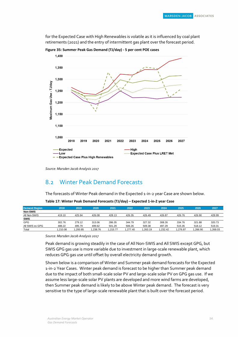
Australian Energy Market Operator Gas Demand Forecasts
54.
for the Expected Case with High Renewables is volatile as it is influenced by coal plant
retirements (2021) and the entry of intermittent gas plant over the forecast period.
Figure 35: Summer Peak Gas Demand (TJ/day) - 5 per cent POE cases
Source: Marsden Jacob Analysis 2017
8.2 Winter Peak Demand Forecasts
The forecasts of Winter Peak demand in the Expected 1-in-2 year Case are shown below.
Table 17: Winter Peak Demand Forecasts (TJ/day) – Expected 1-in-2 year Case
Source: Marsden Jacob Analysis 2017
Peak demand is growing steadily in the case of All Non-SWIS and All SWIS except GPG, but
SWIS GPG gas use is more variable due to investment in large-scale renewable plant, which
reduces GPG gas use until offset by overall electricity demand growth.
Shown below is a comparison of Winter and Summer peak demand forecasts for the Expected
1-in-2 Year Cases. Winter peak demand is forecast to be higher than Summer peak demand
due to the impact of both small-scale solar PV and large-scale solar PV on GPG gas use. If we
assume less large-scale solar PV plants are developed and more wind farms are developed,
then Summer peak demand is likely to be above Winter peak demand. The forecast is very
sensitive to the type of large-scale renewable plant that is built over the forecast period.
Demand Region 2018 2019 2020 2021 2022 2023 2024 2025 2026 2027
Non-SWIS
All Non-SWIS 419.10 425.94 426.08 428.13 426.35 426.49 426.87 426.76 426.90 428.99
SWIS
GPG 302.76 279.12 313.06 286.35 344.79 327.32 308.26 334.76 321.88 320.73
All SWIS ex GPG 488.22 495.79 499.62 501.29 506.26 509.38 497.29 515.35 518.12 519.31
Total 1,210.08 1,200.85 1,238.76 1,215.77 1,277.40 1,263.19 1,232.42 1,276.87 1,266.90 1,269.03
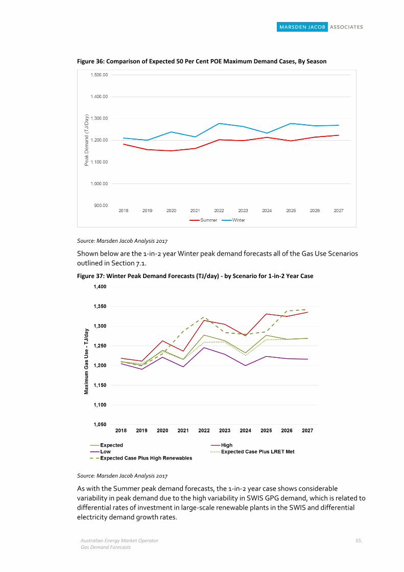
Australian Energy Market Operator Gas Demand Forecasts
55.
Figure 36: Comparison of Expected 50 Per Cent POE Maximum Demand Cases, By Season
Source: Marsden Jacob Analysis 2017
Shown below are the 1-in-2 year Winter peak demand forecasts all of the Gas Use Scenarios
outlined in Section 7.1.
Figure 37: Winter Peak Demand Forecasts (TJ/day) - by Scenario for 1-in-2 Year Case
Source: Marsden Jacob Analysis 2017
As with the Summer peak demand forecasts, the 1-in-2 year case shows considerable
variability in peak demand due to the high variability in SWIS GPG demand, which is related to
differential rates of investment in large-scale renewable plants in the SWIS and differential
electricity demand growth rates.
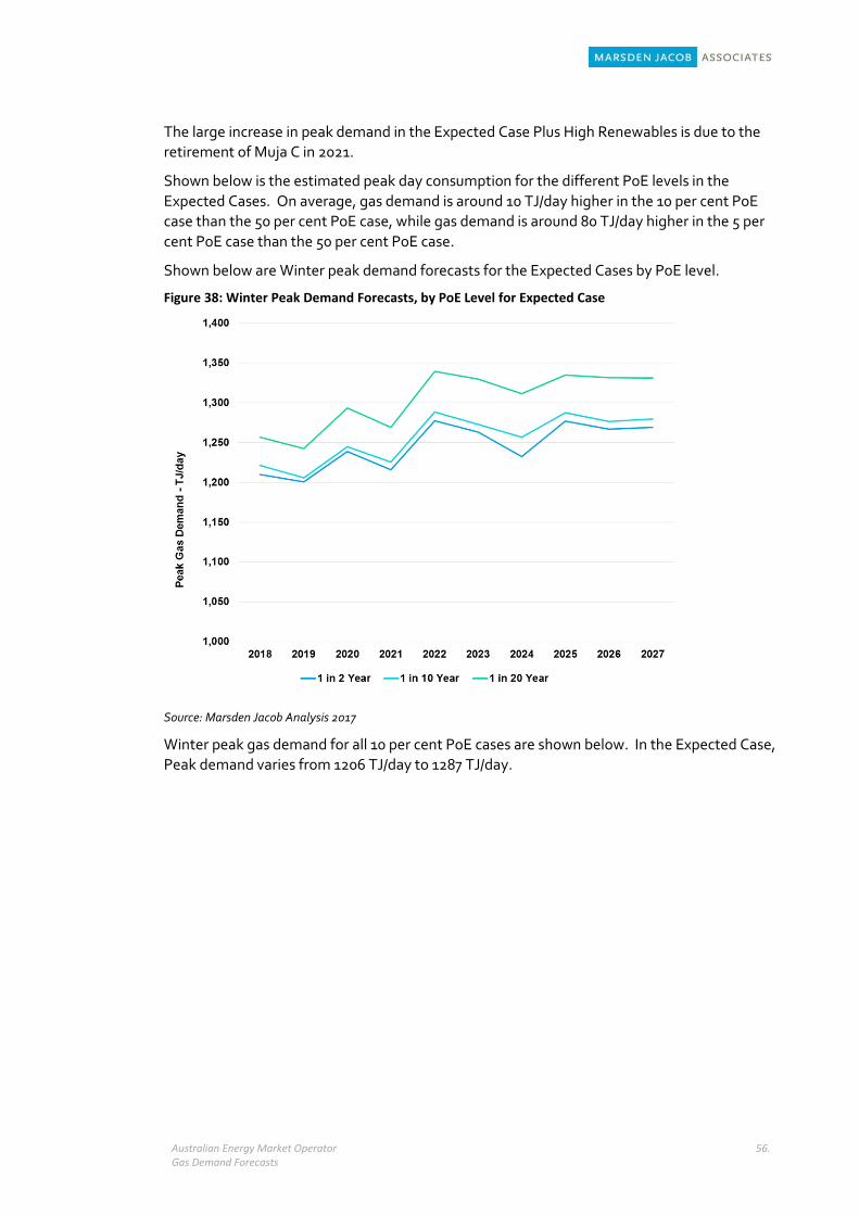
Australian Energy Market Operator Gas Demand Forecasts
56.
The large increase in peak demand in the Expected Case Plus High Renewables is due to the
retirement of Muja C in 2021.
Shown below is the estimated peak day consumption for the different PoE levels in the
Expected Cases. On average, gas demand is around 10 TJ/day higher in the 10 per cent PoE
case than the 50 per cent PoE case, while gas demand is around 80 TJ/day higher in the 5 per
cent PoE case than the 50 per cent PoE case.
Shown below are Winter peak demand forecasts for the Expected Cases by PoE level.
Figure 38: Winter Peak Demand Forecasts, by PoE Level for Expected Case
Source: Marsden Jacob Analysis 2017
Winter peak gas demand for all 10 per cent PoE cases are shown below. In the Expected Case,
Peak demand varies from 1206 TJ/day to 1287 TJ/day.
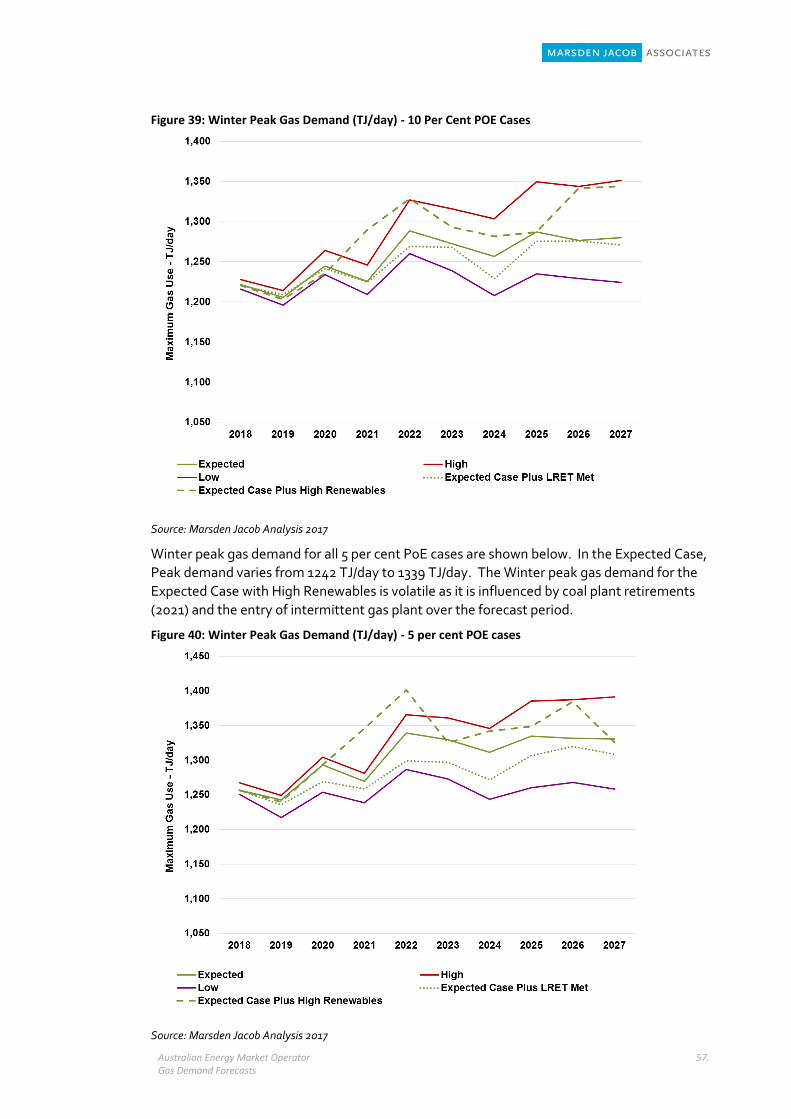
Australian Energy Market Operator Gas Demand Forecasts
57.
Figure 39: Winter Peak Gas Demand (TJ/day) - 10 Per Cent POE Cases
Source: Marsden Jacob Analysis 2017
Winter peak gas demand for all 5 per cent PoE cases are shown below. In the Expected Case,
Peak demand varies from 1242 TJ/day to 1339 TJ/day. The Winter peak gas demand for the
Expected Case with High Renewables is volatile as it is influenced by coal plant retirements
(2021) and the entry of intermittent gas plant over the forecast period.
Figure 40: Winter Peak Gas Demand (TJ/day) - 5 per cent POE cases
Source: Marsden Jacob Analysis 2017
Australian Energy Market Operator Gas Demand Forecasts
58.
Appendix One: SWIS GPG Modelling Assumptions
A1. Inflation
Inflation is measured by changes in the Consumer Price Index (CPI) for Perth on an annual
basis in the model. The assumption used in the analysis is that prices will increase by 2.5 per
cent throughout the forecast period, which is based on the mid-point of the Reserve Bank
inflation target rate.
A2. Exchange Rates
Changes in the value of the Australian Dollar (AUD) can have a significant impact on future
technology costs and domestic gas prices in WA.
First, a falling AUD increases the cost of importing PV equipment (e.g. panels and inverters)
and wind turbines from overseas. Second, increases in the value of the United States Dollar
(USD) against the AUD, increases LNG netback prices and can result in an increase in
domestic gas prices (denominated in AUD).
For our analysis, we have assumed a constant exchange rate of 0.75 USD/AUD for the period
2018 to 2027.
A3. Environmental Policies
The Commonwealth Government is currently influencing future generation investment in
various energy markets through the Large-Scale Renewable Target (LRET) Scheme, the
Small-scale Renewable Energy Scheme (SRES), and the Emissions Reductions Fund (ERF).
A3.1 LRET
The LRET imposes a legislative obligation on electricity retailers (and major customers)12 to
source a given proportion of electricity sales from renewable generation sources. The revised
target for large-scale renewable generation was set at 33,000 GWh by 2020 and must be
supplied each year until the end of calendar year 2030.
To meet their obligations under the scheme, retailers purchase large-scale generation
certificates (LGCs) from accredited renewable generators and then surrender them to the
Clean Energy Regulator (CER). Each certificate represents one megawatt hour (MWh) of
additional renewable energy, are tradable and can be ‘banked' in unlimited quantities for use
in later years. Liable entities can also effectively ‘borrow’ from future certificate surrenders
(this is limited to 10 per cent of an entity’s annual liability). A penalty price (non-tax
deductable) applies to retailers for not submitting required certificates.
Typically, renewable energy projects enter into long term power purchase agreements with
electricity retailers to help underwrite the project. However, there is also a spot LGC market
12 Emissions Intensive Trade Exposed (EITE) industry are exempt from paying the liabilities of the LRET.
Australian Energy Market Operator Gas Demand Forecasts
59.
which enables renewable suppliers and retailers to trade around their renewable energy
contract positions.
In our modelling of GPG gas use in the WEM, we have assumed that WA must meet its pro-
rated share of the Australian wide target for renewable generation by 2020. That is, around
3,267 GWh/annum.
A3.2 Emission Reduction Fund
The Federal Coalition Government abolished carbon pricing and introduced a ‘Direct Action
plan’ in 2014. This involved establishing an ERF, under which the government pays for
emissions abatement through auctions run by the CER. Five auctions were held to April 2017,
spending $2.2 billion to abate 189 million tonnes of carbon13. To date, only one electricity
generation project has successfully participated in the scheme. The project will convert waste
gas from a coal mine to electricity.
In short, the ERF is not having any significant impact on the generation mix in Australia and is
ignored in the WEM modelling.
A3.3 Small-scale Renewable Energy Scheme (SRES)
The SRES places an obligation on retailers to purchase Small-scale Technology Certificates
(STCs) based on a projection of the growth in small-scale technology generators the year
before. A cap on STC prices is set at $40/MWh (tax deductable). STCs are surrendered to the
CER.
The intention is to support the development of small scale technology generation such as
rooftop PV, solar water heaters and heat pumps. Currently the price of STC’s are trading at
near the cap price of $40.
The scheme provides a capital subsidy to residential and commercial customers installing
rooftop PV systems that meet the following criteria:
Solar panel system that has a capacity of no more than 100kW, and a total annual
electricity output less than 250MWh;
Wind system that has a capacity of no more than 10kW, and a total annual electricity
output of less than 25MWh; or
Hydro system that has a capacity of no more than 6.4kW, and a total annual electricity
output of less than 25MWh.
The scheme finishes in December 2030.
A4. Demand and Consumption Forecasts
Annual energy consumption (GWh) and demand forecasts (MW) have been based on the 5-
year average growth rates sourced from the AEMO 2017 Electricity Statement of
Opportunities to project the electricity demand for the whole study period (10 years). This is
due to perceiving AEMO’s 10-year annual growth forecast as too ambitious. Thus, for this
project, the following cases (with the corresponding 10-year average growth rates) were
constructed:
13 Australian Energy Regulator 2017, State of the Energy Market, May. Available from: https://www.aer.gov.au.
[15 September 2017].
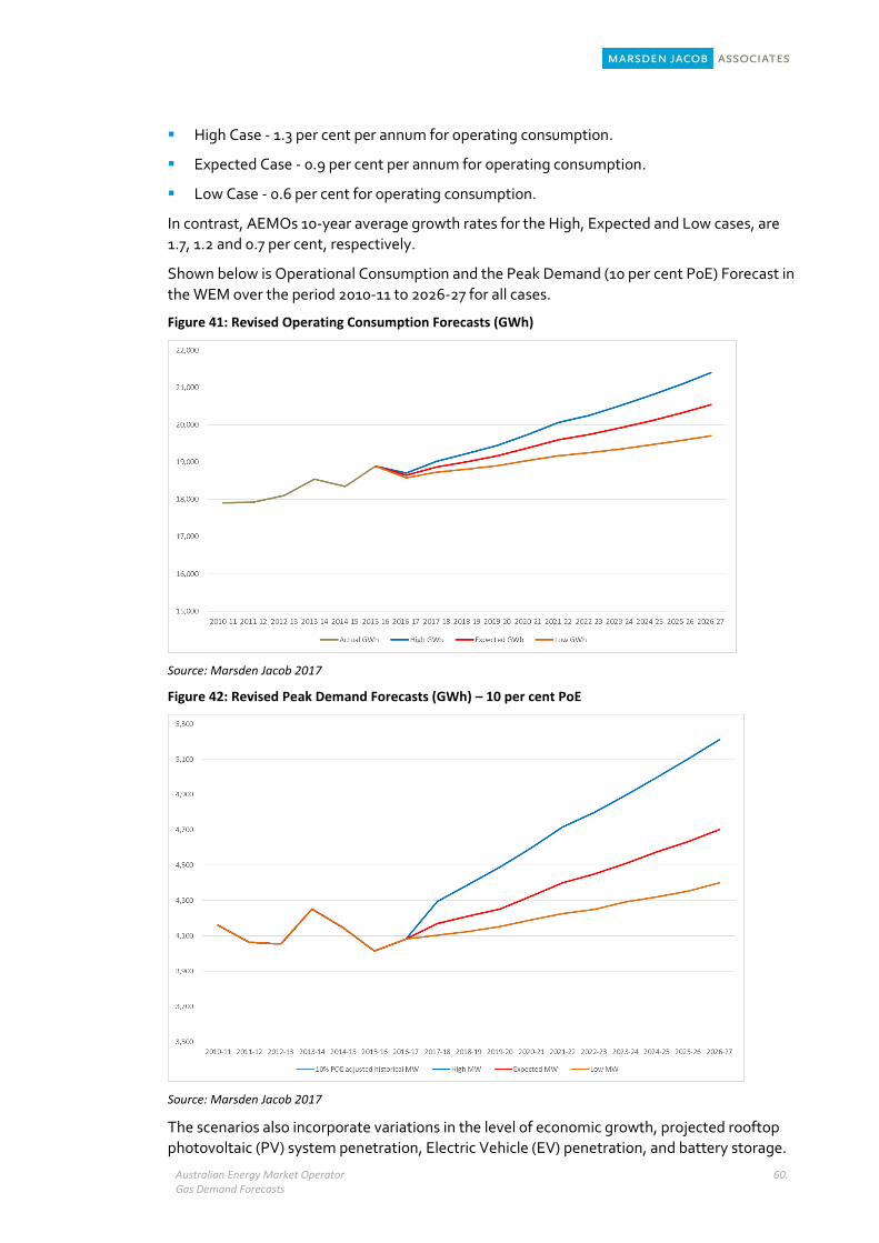
Australian Energy Market Operator Gas Demand Forecasts
60.
High Case - 1.3 per cent per annum for operating consumption.
Expected Case - 0.9 per cent per annum for operating consumption.
Low Case - 0.6 per cent for operating consumption.
In contrast, AEMOs 10-year average growth rates for the High, Expected and Low cases, are
1.7, 1.2 and 0.7 per cent, respectively.
Shown below is Operational Consumption and the Peak Demand (10 per cent PoE) Forecast in
the WEM over the period 2010-11 to 2026-27 for all cases.
Figure 41: Revised Operating Consumption Forecasts (GWh)
Source: Marsden Jacob 2017
Figure 42: Revised Peak Demand Forecasts (GWh) – 10 per cent PoE
Source: Marsden Jacob 2017
The scenarios also incorporate variations in the level of economic growth, projected rooftop
photovoltaic (PV) system penetration, Electric Vehicle (EV) penetration, and battery storage.
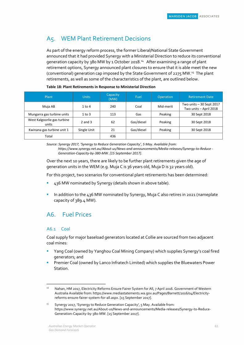
Australian Energy Market Operator Gas Demand Forecasts
61.
A5. WEM Plant Retirement Decisions
As part of the energy reform process, the former Liberal/National State Government
announced that it had provided Synergy with a Ministerial Direction to reduce its conventional
generation capacity by 380 MW by 1 October 2018.14 After examining a range of plant
retirement options, Synergy announced plant closures to ensure that it is able meet the new
(conventional) generation cap imposed by the State Government of 2275 MW.15 The plant
retirements, as well as some of the characteristics of the plant, are outlined below.
Table 18: Plant Retirements in Response to Ministerial Direction
Plant Units Capacity
(MW) Fuel Operation Retirement Date
Muja AB 1 to 4 240 Coal Mid-merit Two units – 30 Sept 2017
Two units – April 2018
Mungarra gas turbine units 1 to 3 113 Gas Peaking 30 Sept 2018
West Kalgoorlie gas turbine units
2 and 3 62 Gas/diesel Peaking 30 Sept 2018
Kwinana gas turbine unit 1 Single Unit 21 Gas/diesel Peaking 30 Sept 2018
Total 436
Source: Synergy 2017, ‘Synergy to Reduce Generation Capacity’, 5 May. Available from: https://www.synergy.net.au/About-us/News-and-announcements/Media-releases/Synergy-to-Reduce -Generation-Capacity-by-380-MW. [15 September 2017].
Over the next 10 years, there are likely to be further plant retirements given the age of
generation units in the WEM (e.g. Muja C is 36 years old, Muja D is 32 years old).
For this project, two scenarios for conventional plant retirements has been determined:
436 MW nominated by Synergy (details shown in above table).
In addition to the 436 MW nominated by Synergy, Muja C also retires in 2021 (nameplate
capacity of 389.4 MW).
A6. Fuel Prices
A6.1 Coal
Coal supply for major baseload generators located at Collie are sourced from two adjacent
coal mines:
Yang Coal (owned by Yanghou Coal Mining Company) which supplies Synergy’s coal fired
generators; and
Premier Coal (owned by Lanco Infratech Limited) which supplies the Bluewaters Power
Station.
14 Nahan, HM 2017, Electricity Reforms Ensure Fairer System for All, 7 April 2016. Government of Western
Australia Available from: https://www.mediastatements.wa.gov.au/Pages/Barnett/2016/04/Electricity-reforms-ensure-fairer-system-for-all.aspx. [15 September 2017].
15 Synergy 2017, ‘Synergy to Reduce Generation Capacity’, 5 May. Available from: https://www.synergy.net.au/About-us/News-and-announcements/Media-releases/Synergy-to-Reduce-Generation-Capacity-by-380-MW. [15 September 2017].
Australian Energy Market Operator Gas Demand Forecasts
62.
In 2014-15, coal production was at 6.5 million tonnes (per annum) and the average price of
coal was $45.90/tonne.16 WA coal has a heating value of 19.5 MJ/tonne, which implied a
delivered price of coal of around $2.36/GJ in 2014-15. Typically, coal contracts are escalated at
CPI.
In October 2014, the Minister for Energy announced an increase in the price paid by Synergy
for coal from Premier Coal of $7/tonne. We have assumed that this price increase takes effect
in 2016-17. Incorporating annual CPI increases and the one-off increase in contract coal price
with Premier Coal, we estimate that prices in 2016-17 will be $2.91/GJ (2017 dollars). Because
of poorer quality coal that has been mined in recent times, we have assumed that the real
price of coal increases by 1 per cent per annum over the forecast period; reflecting the
declining quality of the two existing mines.
A6.2 Long Term Gas Prices
In the long term, gas prices will be less likely to reflect contract values and be reflective of
underlying demand and supply conditions. Given that WA has abundant conventional gas
reserves (92 per cent of Australia’s reserves) and is served by domestic gas only and joint
LNG/domgas facilities, prices will depend on which supply source is ‘marginal’(i.e. which
facility is required to meet incremental demand).
If joint LNG/domgas facilities are the marginal supplier, then domestic gas prices will reflect
the price foregone in making LNG shipments. This is referred to as an LNG netback price and
is outlined below.
In the ASEAN market, gas prices (FOB)17 are oil linked through a formula (s curve):
Gas price (FOB) = slope × oil price (USD/MMBTU) + constant.18
The domestic gas price was determined using the expected future coefficients in the above
equation.
The netback price is based on a financial equivalence of selling gas via export to selling gas
domestically at specified locations. There are two version of netback prices – the short run
and long run netback price.
Once LNG plants are developed, capital costs are sunk and can be excluded from the netback
calculation. That is, only the operating cost of LNG production (~$USD 1/GJ) can be deducted
from Gas Price (FOB). This is referred to as “short-run netback” and is currently the accepted
approach for establishing domestic gas prices on the eastern seaboard.
If the productions plants are not yet developed, capital costs are not sunk and can be included
in the netback calculation. That is, $USD 5/GJ can be deducted to calculate the long run
netback price of gas. This represents the maximum cost gas prior to the investment decision
and is referred to as the “long-run netback price”.
Using netback prices, we can establish a range of prices that may be relevant for establishing
long run domestic gas prices from joint LNG and domestic gas facilities.
16 Department of Mines, Industry Regulation and Safety 2015, Statistics Digest 20114-15, Government of
Western Australia. Available from: http://www.dmp.wa.gov.au/documents/Stats_Digest_2014-15.pdf. [15
September 2017].
17 Free on Board
18 In our model, the slope = 0.13 and the constant = 0.3.
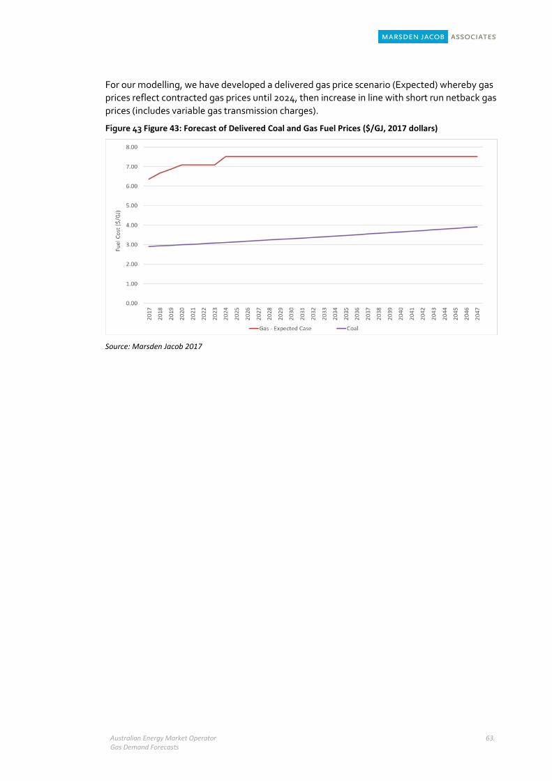
Australian Energy Market Operator Gas Demand Forecasts
63.
For our modelling, we have developed a delivered gas price scenario (Expected) whereby gas
prices reflect contracted gas prices until 2024, then increase in line with short run netback gas
prices (includes variable gas transmission charges).
Figure 43 Figure 43: Forecast of Delivered Coal and Gas Fuel Prices ($/GJ, 2017 dollars)
Source: Marsden Jacob 2017