The determinants of economic growthin European regions∗

Jesus Crespo Cuaresma†

WU, IIASA, WIC and WIFO

Gernot Doppelhofer‡

NHH

Martin Feldkircher§

OeNB

Abstract

This paper uses Bayesian Model Averaging (BMA) to find robust determinants ofeconomic growth in a new dataset of 255 European regions between 1995 and 2005. Thepaper finds that income convergence between countries is dominated by the catching-up ofregions in new member states in Central and Eastern Europe (CEE), whereas convergencewithin countries is driven by regions in old EU member states. Regions containing capitalcities are growing faster, particularly in CEE countries, as do regions with a large shareof workers with higher education. The results are robust to allowing for spatial spilloversamong European regions.

Keywords: Bayesian Model Averaging (BMA), Spatial Autoregressive (SAR) model, deter-minants of economic growth, European regions.

JEL Classifications: C11, C21, R11, O52.

∗ This paper was prepared as a background study to the statistical analysis on the factors of regional economic growth coor-dinated by The Vienna Institute for International Economic Studies (www.wiiw.ac.at) in the framework of the project ”Analysisof the Main Factors of Regional Growth: An in-depth study of the best and worst performing European regions” (contract no.2007.CE.16.0.AT.029). Financial support from European Community, DG Regional Policy, is gratefully acknowledged. The au-thors would like to thank two anonymous referees as well as Carlo Altavilla, Harald Badinger, Roger Bivand, Manfred Fischer,Sylvia Fruhwirth-Schnatter, Jim LeSage, Robert Stehrer, Stefan Zeugner and participants of the WIIW Workshop on RegionalGrowth, CESifo Macro Area Conference, III World Conference of Spatial Econometrics in Barcelona and the Bergen Econometricsgroup for helpful comments. The opinions in this paper are those of the authors and do not necessarily coincide with those of theOesterreichische Nationalbank or the EU Commission.†Department of Economics, Vienna University of Economics and Business (WU). Augasse 2-6, 1090 Vienna,

Austria; World Population Program, International Institute of Applied Systems Analysis (IIASA), WittgensteinCentre for Demography and Global Human Capital (WIC) and Austrian Institute for Economic Research(WIFO). jcrespo@wu.ac.at.‡Department of Economics, Norwegian School of Economics (NHH). Helleveien 30, 5045 Bergen, Norway.

gernot.doppelhofer@nhh.no.§Oesterreichische Nationalbank, Otto-Wagner-Platz 3, 1090 Vienna, Austria.

martin.feldkircher@oenb.at.

1

1 Introduction

This paper investigates determinants of regional economic growth based on a new data set of255 EU regions at the NUTS (Nomenclature of Territorial Units) level 2 of disaggregation span-ning the period 1995-2005. The paper uses Bayesian Model Averaging to assess the robustnessof growth determinants in a systematic way, drawing explicit attention to the spatial interac-tions among European regions. The paper also investigates potential parameter heterogeneitydue to the inclusion of regions from member countries in Central and Eastern Europe, whichexperienced a deep economic transformation process in the period under study. This studypresents to the best knowledge of the authors the most comprehensive empirical investigationhitherto of the robustness of economic growth determinants in European regions.

Following Barro (1991), several studies have included a large number of explanatory variablesin so-called ’kitchen sink’ regressions based on cross-country data sets.1 A problem with thisapproach is that theories of economic growth are often not mutually exclusive and the valid-ity of one theory does not necessarily imply that another theory is false. Brock and Durlauf(2001) refer to this problem as ’open-endedness’ of growth theories. Empirical models of eco-nomic growth are therefore plagued by problems of model uncertainty concerning the choiceof explanatory variables and model specification. Levine and Renelt (1992) questioned therobustness of growth determinants by using a version of extreme bounds analysis (EBA) devel-oped by Leamer (1983). Sala-i-Martin (1997) criticizes the extreme bounds as being too strictand proposes to analyze the entire distribution of coefficients of interest, which supported theimportance of a wider set of growth determinants.

A recent and quickly growing literature addresses this problem of model uncertainty in growthempirics systematically by using Bayesian Model Averaging (henceforth BMA).2 Fernandezet al. (2001b) investigate the robustness of the growth determinants by using BMA on thedataset collected by Sala-i-Martin (1997). Following Leamer (1978), Sala-i-Martin et al. (2004)use Bayesian Averaging of Classical Estimates (BACE) which uses least-squares (classical)estimates and sample-dominated model weights that are positively related to the Bayesian In-formation Criterion (BIC) developed by Schwarz (1978).3 Other studies study the importanceof parameter heterogeneity in the uncertain growth process (see Crespo Cuaresma and Doppel-hofer (2007), or Doppelhofer and Weeks (2009)). Despite this focus on various aspects of modeluncertainty, the literature paid little attention to regional aspects of the uncertain growth pro-cess.

A number of recent studies have investigated model uncertainty in the context of robustnessof growth determinants and income convergence patterns at the regional level. The empiricalassessment of regional growth determinants has the added complication that spatial correlationis present in the data to a much higher extent than in cross-country data. Recently, a branch

1Barro and Sala-i-Martin (2004) give an excellent overview of empirical analysis for regional data (Chapter11) and cross-sections of countries (Chapter 12).

2See Hoeting et al. (1999) for an excellent tutorial introduction to BMA and the survey by Doppelhofer(2008) that discusses both Bayesian and frequentist techniques.

3Raftery (1995) also proposes to combine BIC model weights and maximum likelihood estimates for modelselection, with a method which differs from Sala-i-Martin et al. (2004) in the specification of prior probabilitiesover the model space and sampling method.

2

of literature has developed Bayesian tools for the analysis of spatially correlated data undermodel uncertainty. LeSage and Parent (2007) give an excellent introduction to BMA for spatialeconometric models, and LeSage and Fischer (2008) apply BMA to investigate determinants ofincome in EU regions, with particular emphasis on sectoral factors. Knowledge spillovers frompatent activity between EU regions, one of the most important growth determinants accordingto endogenous growth theory, is the focus of the analysis in LeSage and Parent (2008).

Many other empirical studies analyze regional growth determinants and income convergencein Europe but do not deal with the issue of model uncertainty and spatial spillovers simul-taneously.4 Boldrin and Canova (2001), for instance, investigate income convergence in EUregions and its relationship to regional policies, concluding with a critical assessment of re-gional economic policies. Becker et al. (2008) find evidence for growth, but not employmenteffects of regions receiving structural funds as so-called Objective 1 regions. Canova (2004)and Ertur et al. (2006) test for convergence clubs in European regions and finds evidence forconvergence poles characterized by different economic conditions. Corrado et al. (2005) usean alternative technique to identify clusters of convergence in European regions and sectors.Carrington (2003) investigates convergence among EU regions and finds evidence of negativespatial spillovers among neighboring regions. Basile (2008) estimates a semiparametric spa-tial model for European regions and finds evidence for nonlinear effects associated with initialincome and human capital investments, as well as some indication for global and local spillovers.

This paper contributes to the literature on determinants of regional growth in several aspects.First, we investigate a set of 50 possible growth determinants in 255 NUTS 2 regions of theEU. Compared to the limited set of variables considered in the existing empirical literature, thepaper rigorously assesses model uncertainty over a much larger set of determinants of regionalgrowth. Second, the paper uses BMA to investigate the robustness of determinants of regionalgrowth between and within countries, as well as allowing for spatial spillovers. In particular,three different specifications are estimated to describe the growth process in EU regions: (1)the baseline case of a pure cross-section of EU regions, (2) the baseline plus country fixed effects,and (3) the baseline combined with a spatial autoregressive (SAR) structure.5 Third, this paperuses a particular prior structure for interaction terms that fulfills the strong heredity principleput forward by Chipman (1996) when designing priors over the model space for related variables(see Crespo Cuaresma (2011) for a recent discussion on the use of interaction terms in BMA).Thus, the specification allows for heterogeneous effects of selected growth determinants in recentaccession countries in Central and Eastern Europe (CEE) – Bulgaria, Czech Republic, Estonia,Hungary, Latvia, Lithuania, Poland, Romania, Slovenia and Slovak Republic –, and also incapital cities. Finally, the paper allows for uncertainty over spatial weights by conducting asensitivity analysis with respect to alternative spatial distance measures.

The main findings of the paper can be summarized as follows:

1. Conditional income convergence is a robust driving force of income growth across Euro-pean regions. In the cross-section of regions, there is evidence for conditional convergencewith a speed of around two percent. However, the precision of the estimated speed of con-vergence is strongly affected by the growth experience of CEE countries. The convergenceprocess between European regions is dominated by the catching up process of regions in

4For an overview of convergence in EU regions at NUTS-2 level see European Commission (2008).5See Anselin (1988) and LeSage and Pace (2009) for textbook discussions of the SAR model.

3

’new’ EU member states in CEE countries, whereas convergence within countries is mostlya characteristic of regions in ’old’ EU member states.

2. Regions with capital cities grow on average by one percentage point faster than non-capitalcity regions. This result, however, hides very strong differences between the experience ofold and new EU member states. Regions containing capital cities in Central and EasternEurope grew on average 1.8 percentage points faster, compared to only 0.4 percentagegrowth bonus in capital regions in old EU member states. Together with the observedconvergence patterns in EU regions, this observations lends empirical support to theso-called ’Williamson hypothesis’. According to Williamson (1965), economic growthconcentrates in regions with urban agglomerations as the catching-up process progresses,reverting the process in later stages of development. While this effect is very robust, itshould be noted that these growth patterns may be related to the fact that the periodunder analysis (1995-2005) was characterized by rapid income growth in Eastern Europe.

3. Human capital, measured as population share of workers with higher (tertiary) education,has a robust positive association with regional economic growth. The estimates implythat an increase of 10 percent in the population share of workers with higher education isassociated with a 0.6 percentage points higher annual growth rate of GDP per capita. Thepositive effect of human capital remains a robust determinant of regional growth withincountries, but the parameter is not as well estimated as in the case without fixed countryeffects.

4. Allowing for spatial autocorrelation a priori, the paper finds evidence for positive spatialspillovers (growth clusters) in EU regions. However, spatial lags of growth determinantsunder consideration do not play a substantial role in explaining economic growth in Euro-pean regions. The spatial spillovers are not operating through the explanatory variablesat hand, but rather reflect some residual spatial effects which cannot be accounted by theexplanatory variables or their spatial lags.

5. Statistical and economic inference on the determinant of regional economic growth isrobust to alternative spatial weighting schemes for the economic growth spillovers. Thisrobustness is also supported by a recent study by Crespo Cuaresma and Feldkircher(2010), which uses a different method to assess spatial link uncertainty in the regionalgrowth process and investigates a wider set of weighting matrices.

The paper is structured as follows. Section 2 presents the setting of the BMA exercise carriedout in the paper. Section 3 presents the empirical results concerning the robustness of growthdeterminants in the EU at the regional level and checks for the robustness of the results to varia-tions in the spatial weighting matrix and in the nature of the potential parameter heterogeneity.Section 4 concludes.

2 The econometric model: Specification and prior struc-

tures

The robustness of regional growth determinants is analyzed using three different specifications.First, the baseline case pools the full cross-section of regions, taking into account variation ofregional growth both between and within countries. Second, the baseline case with country

4

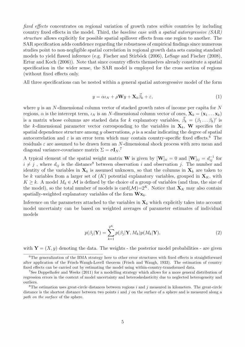
fixed effects concentrates on regional variation of growth rates within countries by includingcountry fixed effects in the model. Third, the baseline case with a spatial autoregressive (SAR)structure allows explicitly for possible spatial spillover effects from one region to another. TheSAR specification adds confidence regarding the robustness of empirical findings since numerousstudies point to non-negligible spatial correlation in regional growth data sets causing standardmodels to yield flawed inference (e.g. Fischer and Stirbock (2006), LeSage and Fischer (2008),Ertur and Koch (2006)). Note that since country effects themselves already constitute a spatialspecification in the wider sense, the SAR model is employed for the cross section of regions(without fixed effects only.

All three specifications can be nested within a general spatial autoregressive model of the form

y = αιN + ρWy + Xk~βk + ε, (1)

where y is an N -dimensional column vector of stacked growth rates of income per capita for Nregions, α is the intercept term, ιN is an N -dimensional column vector of ones, Xk = (x1 . . .xk)

is a matrix whose columns are stacked data for k explanatory variables, ~βk = (β1 . . . βk)′ is

the k-dimensional parameter vector corresponding to the variables in Xk, W specifies thespatial dependence structure among y observations, ρ is a scalar indicating the degree of spatialautocorrelation and ε is an error term which may contain country-specific fixed effects.6 Theresiduals ε are assumed to be drawn form an N -dimensional shock process with zero mean anddiagonal variance-covariance matrix Σ = σIN .7

A typical element of the spatial weight matrix W is given by [W]ii = 0 and [W]ij = d−1ij for

i 6= j , where dij is the distance8 between observation i and observation j. The number andidentity of the variables in Xk is assumed unknown, so that the columns in Xk are taken tobe k variables from a larger set of (K) potential explanatory variables, grouped in XK , withK ≥ k. A model Mk ∈M is defined by the choice of a group of variables (and thus, the size ofthe model), so the total number of models is card(M)=2K . Notice that XK may also containspatially-weighted explanatory variables of the form Wxk.

Inference on the parameters attached to the variables in Xk which explicitly takes into accountmodel uncertainty can be based on weighted averages of parameter estimates of individualmodels

p(βj|Y) =2K∑k=1

p(βj|Y,Mk)p(Mk|Y), (2)

with Y = (X, y) denoting the data. The weights - the posterior model probabilities - are given

6The generalization of the BMA strategy here to other error structures with fixed effects is straightforwardafter application of the Frisch-Waugh-Lovell theorem (Frisch and Waugh, 1933). The estimation of countryfixed effects can be carried out by estimating the model using within-country-transformed data.

7See Doppelhofer and Weeks (2011) for a modelling strategy which allows for a more general distribution ofregression errors in the context of model uncertainty and heteroskedasticity due to neglected heterogeneity andoutliers.

8The estimation uses great-circle distances between regions i and j measured in kilometers. The great-circledistance is the shortest distance between two points i and j on the surface of a sphere and is measured along apath on the surface of the sphere.

5

by

p(Mj|Y) =p(Y|Mj)p(Mj)∑2K

k=1 p(Y|Mk)p(Mk). (3)

For the sake of illustration, consider the particular case of two models. In this case, the formerexpression boils down to the product of the Bayes factor p(Y|M1)/p(Y|M2) with the prior oddsp(M1)/p(M2). Since the Bayes factor involves the marginal likelihoods unter the respectivemodels it serves as a measure of differences in fit (with a penalty for model size embedded).

Model weights can thus be obtained using the marginal likelihood of each individual modelafter eliciting a prior over the model space. The marginal likelihood of model Mj is in turngiven by

p(Y|Mj) =

∫ ∞0

∫ ∞−∞

∫ ∞−∞

∫ ∞−∞

p(Y|α, ~βk, ρ, σ,Mj)p(α, ~βk, ρ, σ|Mj) dα d~βk dρ dσ. (4)

The priors for the regression model provided in equation (1) are elicited by using a noninforma-tive improper prior on the parameters common in all models, α and σ, and by using so-calledg-prior (Zellner, 1986) on the β-coefficients:

p(~βk|α, ρ, σ,Mj) ∼ N(βk, σ2g(X′kXk)

−1),

Note that g scales up prior variance of β-coefficients reflecting the strength of the prior beliefregarding the regression coefficients. In the application, prior coefficient means are set to zeroreflecting an agnostic prior about the sign of coefficients, βk = ~0, and following Fernandez et al.(2001a) the hyperparameter for the g-prior is set to g = max{N,K2}, which in our case impliesthat g = K2 for all the settings presented below. This so-called benchmark prior over g impliesfor linear regression models that the relative size of the sample as compared to the number ofcandidate regressors will determine whether models are compared based on the BIC (BayesianInformation Criterion, Schwarz (1978)) or RIC (Risk Inflation Criterion, Foster and George

(1994)). As in LeSage and Parent (2007), this paper combines a benchmark prior for ~βk witha beta prior distribution for ρ.

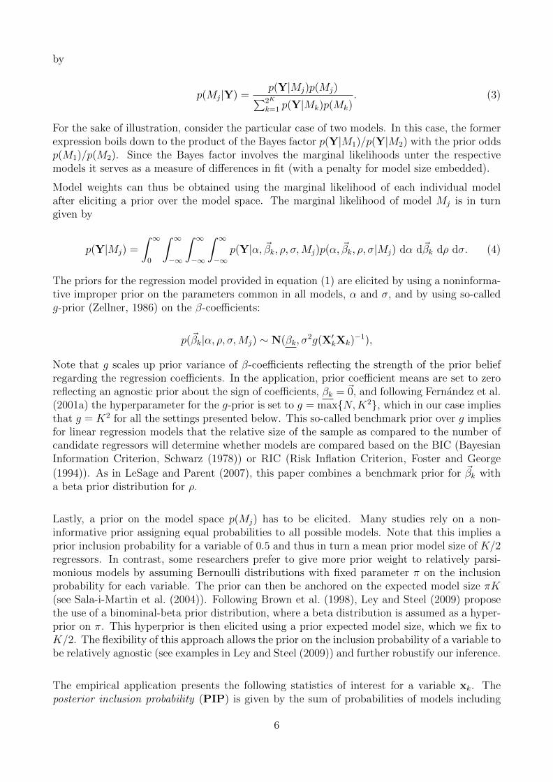
Lastly, a prior on the model space p(Mj) has to be elicited. Many studies rely on a non-informative prior assigning equal probabilities to all possible models. Note that this implies aprior inclusion probability for a variable of 0.5 and thus in turn a mean prior model size of K/2regressors. In contrast, some researchers prefer to give more prior weight to relatively parsi-monious models by assuming Bernoulli distributions with fixed parameter π on the inclusionprobability for each variable. The prior can then be anchored on the expected model size πK(see Sala-i-Martin et al. (2004)). Following Brown et al. (1998), Ley and Steel (2009) proposethe use of a binominal-beta prior distribution, where a beta distribution is assumed as a hyper-prior on π. This hyperprior is then elicited using a prior expected model size, which we fix toK/2. The flexibility of this approach allows the prior on the inclusion probability of a variable tobe relatively agnostic (see examples in Ley and Steel (2009)) and further robustify our inference.

The empirical application presents the following statistics of interest for a variable xk. Theposterior inclusion probability (PIP) is given by the sum of probabilities of models including

6

variable xk. A PIP close to unity indicates the importance of the respective variable in ex-plaining the process of regional growth. Note that the PIP can be interpreted as measure ofevidence of including the variable contingent on other variables being included. The posteriormean of the distribution of βk (PM) is the sum of model-weighted means of the model specificposterior distributions of the parameter:

E(βk|Y) =2K∑l=1

p(Ml|Y)E(βk|Y,Ml).

The posterior variance of βk is the model-weighted sum of conditional variances plus an addi-tional term capturing the uncertainty of the (estimated) posterior mean across models

var(βk|Y) =2K∑l=1

p(Ml|Y)var(βk|Y,Ml) +

+2k∑l=1

p(Ml|Y)(E(βk|Y,Ml)− E(βk|Y))2.

The posterior standard deviation is defined accordingly as PSDk =√

var(βk|Y).

The posterior distributions of the β-parameters for the SAR specification are calculated forthe ρ that maximizes the integrated likelihood p(ρ|Y,W) (equation (A.2) in the TechnicalAppendix) over a grid of ρ values. The posterior distributions of interest over the model spacecan be then obtained using Markov Chain Monte Carlo Model Composition (MC3) methods ina straightforward manner (see LeSage and Parent (2007)). In particular, a random-walk step isused in every replication of the MC3 procedure, constructing an alternative model to the activeone in each step of the chain by adding or subtracting a regressor from the active model. Thechain then moves to the alternative model with probability given by the product of Bayes factorand prior odds resulting from the binomial-beta prior distribution. The posterior inferenceis based on the models visited by the Markov chain instead of on the complete (potentiallyuntractable) model space (see Fernandez et al. (2001a) for a more detailed description of thisstrategy). The Technical Appendix describes the implemented BMA procedure and the MC3

sampling method implemented in the empirical analysis in more detail.

For the evaluation of potential nonlinear effects by inclusion of interaction terms, the MC3

method is adapted as follows to ensure that Chipman’s (1996) strong heredity principle isfulfilled. Positive prior inclusion probability is assigned only to models which include no inter-action terms or models with interaction terms, but interacted variables also appearing linearly.In practice, an MC3 sampler is implemented which adds the individual interacted variableslinearly to those models in which the interaction is included, so as to ensure that only theindependent effect of the interaction is evaluated. This approach imposes a particular prior dis-tribution over the model space, removing the prior probability mass from all the models whereinteractions are present, but the corresponding linear terms are not part of the model. Thisprior probability mass is correspondingly redistributed to models where the interaction appearstogether with the interacted variables and can thus be properly interpreted. Crespo Cuaresma(2011) presents evidence that this type of interaction sampling method has better properties

7

than standard MC3 in the sense that the latter may spuriously detect interaction effects whichare not present in the data. This sampling procedure implies a particular dilution prior overthe model space which assigns zero prior probability to models containing interactions whoseparent variables are missing in the specification.9 This prior structure ensures that the inter-active effects found relate to the pure interaction term and are not masking the effect of the(potentially correlated) parent variables.

3 Empirical results

The dataset covers information on 255 European regions listed in Table B.1. The Data Appendixlists the full set of regions and available variables, together with a brief definition, descriptivestatistics and the source for each one of them. The dependent variable refers to observations ofthe average annual growth rate of each region in the period 1995-2005, deflated using nationalprice data.10 Note that three variables expressed in shares serve as reference group (denotedby asterisks (*) in Table B.2) and are therefore not included in the regressions. This results in50 explanatory variables which can be roughly divided into several thematic groups:

1. Factor accumulation and convergence: These variables correspond to the usual economicgrowth determinants implied by neoclassical growth models (initial income, populationgrowth, and investment in physical capital);

2. Human capital: Population shares of workers with high (tertiary), medium (secondary)and low (primary) educational attainment, as well as a life long learning variable;

3. Technological innovation: Patent statistics, as well as the share of workers employed inthe science and technology sector;

4. Sectoral structure and employment: Sectoral shares in GDP; employment, unemploymentand activity rates;

5. Infrastructure: Firm access to websites and telecommunications; access to sea, roads, airand rail transport;

6. Socio-geographical: Settlement structure; output, employment and population density;geographical location variables; Objective 1 regions11; capital city region.

All explanatory variables are measured at (or as close as possible) to the beginning of thesample period 1995 to capture the initial state of EU regions. Endogeneity in the relationshipbetween regional growth and several potential determinants may be a concern in empiricalwork on economic growth at the subnational level. The dataset therefore measures regressorsat (or as close as possible to) the beginning of the sample period to partly mitigate problems ofendogeneity. The estimation by least squares therefore treats the regressors as predetermined.

9See the Technical Appendix for details.10The starting year of the observation period is determined by the lack of reliable and comparable regional

data for the first part of the 1990s for Central and Eastern European countries.11Structural funds programs allocating transfers to NUTS-2 regions and associated classification into so-called

Objective 1 regions are not considered for obvious concerns about endogeneity. A recent study by Becker et al.(2008) uses a regression discontinuity approach to identify the impact of structural funds and finds growth, butno employment effects.

8

This - as well as the use of country fixed effects in the within specification - should reducethe problem of endogeneity that is potentially associated with the use of some of the potentialgrowth determinants. Given this maintained assumption, one should be careful not to attach adirect causal interpretation to the estimated effects. Alternatively, a researcher might considerto use lagged values of regressors as potential instruments, although the high persistence ofmany regressors could imply the well-known weak instruments problem. Combined with likelymeasurement errors of regional growth and its determinants, Hauk and Wacziarg (2009) warnagainst the naive use of lagged values of regressors as instrumental variables, since this couldimply larger biases than the much simpler ordinary least-squares estimator considered in thispaper.12

The paper evaluates the robustness of potential growth determinants for European regions byusing BMA in three different specifications: (1) the baseline case pools all regions and ana-lyzes variation across regions and between countries; (2) the baseline plus country fixed effectsfocusses on regional variation within countries of the EU 27; (3) the baseline combined witha spatial autoregressive (SAR) specification is employed to capture growth spillovers amongEU regions with different choices for the spatial weight matrix W. The evaluation of nonlin-earities in the regional growth processes is assessed using interactions of pairs of variables asextra explanatory variables. Model averaging in a model space which includes specificationswith interacted variables takes place imposing the strong heredity principle by modifying thestandard MC3 sampler as described in the Technical Appendix.

We present the empirical findings based on the three different model specifications discussedabove. In the tables we report the posterior inclusion probabilities (PIP) of each regressor,together with the mean (PM) and standard deviation (PSD) of the posterior distribution forthe associated parameter. The results are obtained from three million draws of the MC3 sampler,after a burn-in phase of two million iterations. We use in all cases a binomial-beta prior wherethe expected model size equals K/2 regressors.13 For easier readability, we restrict the variablesshown in the tables to those that have a posterior inclusion probability above 0.5 (which we labelrobust in at least one of the specifications used.14 Such robust variables have a higher inclusionprobability after observing the data than their prior inclusion probability. One can use the scalesproposed by Kass and Raftery (1995), to classify evidence of robustness of growth determinantsinto four categories (see also Eicher et al. (2011)): weak (50-75% PIP), substantial (75-95%),strong (95-99%) and decisive (99%+) evidence.15 Alternatively, the economic significance ofgrowth determinants can also be assessed by looking at their transformed coefficients, definedas PM/PSD. Masanjala and Papageorgiou (2008), for instance, label explanatory variables withabsolute values of transformed coefficients greater than 1.3 as ’effective’.16

12Unfortunately, our dataset does not contain lagged observations of the data, we therefore leave extensionsin this dimension to future work.

13The hyperparameters for the binomial-beta distribution are set to a = b = 1.14The full set of results is available from the authors upon request.15Note that this scale is based on a prior inclusion probability of 0.5 for each regressor which is implied by

the binomial-beta prior anchored around an expected model size of K/2. The variables are sorted by posteriorinclusion probabilities in the first set of columns in each Table of results.

16Brock and Durlauf (2001) provide decision-theoretic foundations for using such transformed coefficients.Even though the particular cutoff values for PIPs and transformed coefficients are specific to the assumed priorstructure, the results are robust to alternative choice of prior parameters.

9

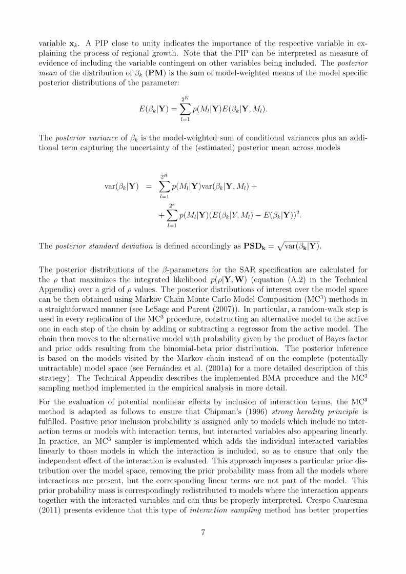
Model 1 Model 2 Model 3PIP PM PSD PIP PM PSD PIP PM PSD

Capital city 1.000 0.018 0.002 0.984 0.011 0.003 1.000 0.004 0.003Initial income 1.000 -0.020 0.002 0.245 -0.003 0.005 0.387 -0.004 0.005Higher education workers (share) 0.977 0.048 0.012 0.999 0.063 0.011 0.996 0.053 0.010

0.001 0.003 0.000 0.001Distance to Frankfurt 0.005 0.001 0.000 0.388 0.001 0.000 0.590 0.001 0.000CEE Dummy InteractionsCEE dummy 0.982 0.019 0.006 1.000 0.016 0.005CEE dummy × Capital city 0.996 0.018 0.004Share of post. prob. (best model) 0.53 0.31 0.46Share of post. prob. (best 25 models) 0.89 0.86 0.86Share of post. prob. (best 50 models) 0.92 0.90 0.90

PIP stands for ’posterior inclusion probability’, PM stands for ’posterior mean’ and PSD stands for ’posterior standard deviation’.

All calculations based on MC3 sampling with 2,000,000 burn-ins and 3,000,000 posterior draws. Model 1: Cross section of regions

(baseline). Model 2: Cross section of regions including the CEE dummy variable and related interaction terms. Model 3: Cross

section of regions further including the interaction term of the capital city dummy with the CEE dummy variable. Under models

2 and 3 the ’strong heredity prior’ has been employed.

Table 1: BMA results for baseline setting

Model 1 Model 2 Model 3Intercept 0.205∗∗∗ 0.001 0.001

(0.012) (0.002) (0.002)Capital city 0.018∗∗∗ 0.009∗∗∗ 0.009∗∗∗

(0.002) (0.002) (0.002)Initial income -0.020∗∗∗

(0.001)Higher education workers (share) 0.048∗∗∗ 0.059∗∗∗ 0.059∗∗∗

(0.009) (0.009) (0.009)Distance to Frankfurt 0.001∗∗∗ 0.001∗∗∗

(0.000) (0.000)CEE dummy 0.023∗∗∗ 0.023∗∗∗

(0.002) (0.002)Observations 255 255 255Adjusted R2 0.567 0.597 0.597Moran’s I test (p-value) 0.001 0.011 0.011Shapiro-Wilk test (p-value) 0.001 0.001 0.001

Standard errors in parenthesis, ∗∗∗ indicates significance at the 1% level. Moran’s I test and the Shapiro-Wilk test have as a null

hypothesis the absence of spatial autocorrelation and residual normality, respectively.

Table 2: Models with highest posterior probability: baseline setting

10

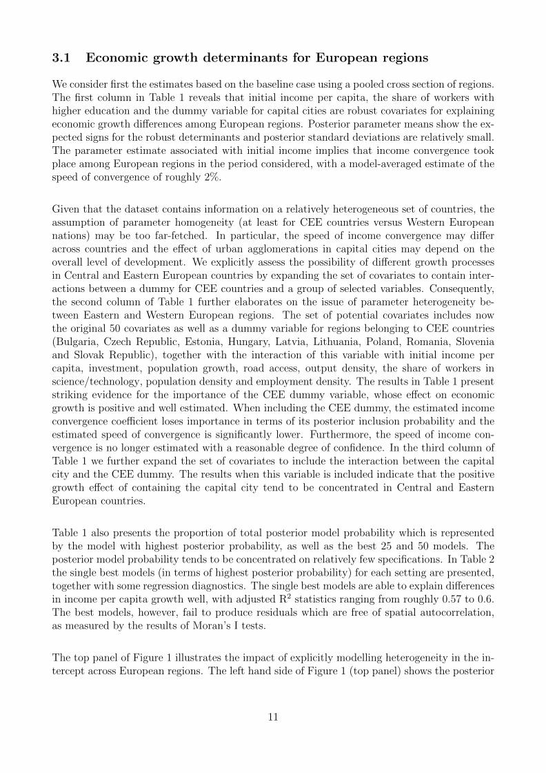
3.1 Economic growth determinants for European regions

We consider first the estimates based on the baseline case using a pooled cross section of regions.The first column in Table 1 reveals that initial income per capita, the share of workers withhigher education and the dummy variable for capital cities are robust covariates for explainingeconomic growth differences among European regions. Posterior parameter means show the ex-pected signs for the robust determinants and posterior standard deviations are relatively small.The parameter estimate associated with initial income implies that income convergence tookplace among European regions in the period considered, with a model-averaged estimate of thespeed of convergence of roughly 2%.

Given that the dataset contains information on a relatively heterogeneous set of countries, theassumption of parameter homogeneity (at least for CEE countries versus Western Europeannations) may be too far-fetched. In particular, the speed of income convergence may differacross countries and the effect of urban agglomerations in capital cities may depend on theoverall level of development. We explicitly assess the possibility of different growth processesin Central and Eastern European countries by expanding the set of covariates to contain inter-actions between a dummy for CEE countries and a group of selected variables. Consequently,the second column of Table 1 further elaborates on the issue of parameter heterogeneity be-tween Eastern and Western European regions. The set of potential covariates includes nowthe original 50 covariates as well as a dummy variable for regions belonging to CEE countries(Bulgaria, Czech Republic, Estonia, Hungary, Latvia, Lithuania, Poland, Romania, Sloveniaand Slovak Republic), together with the interaction of this variable with initial income percapita, investment, population growth, road access, output density, the share of workers inscience/technology, population density and employment density. The results in Table 1 presentstriking evidence for the importance of the CEE dummy variable, whose effect on economicgrowth is positive and well estimated. When including the CEE dummy, the estimated incomeconvergence coefficient loses importance in terms of its posterior inclusion probability and theestimated speed of convergence is significantly lower. Furthermore, the speed of income con-vergence is no longer estimated with a reasonable degree of confidence. In the third column ofTable 1 we further expand the set of covariates to include the interaction between the capitalcity and the CEE dummy. The results when this variable is included indicate that the positivegrowth effect of containing the capital city tend to be concentrated in Central and EasternEuropean countries.

Table 1 also presents the proportion of total posterior model probability which is representedby the model with highest posterior probability, as well as the best 25 and 50 models. Theposterior model probability tends to be concentrated on relatively few specifications. In Table 2the single best models (in terms of highest posterior probability) for each setting are presented,together with some regression diagnostics. The single best models are able to explain differencesin income per capita growth well, with adjusted R2 statistics ranging from roughly 0.57 to 0.6.The best models, however, fail to produce residuals which are free of spatial autocorrelation,as measured by the results of Moran’s I tests.

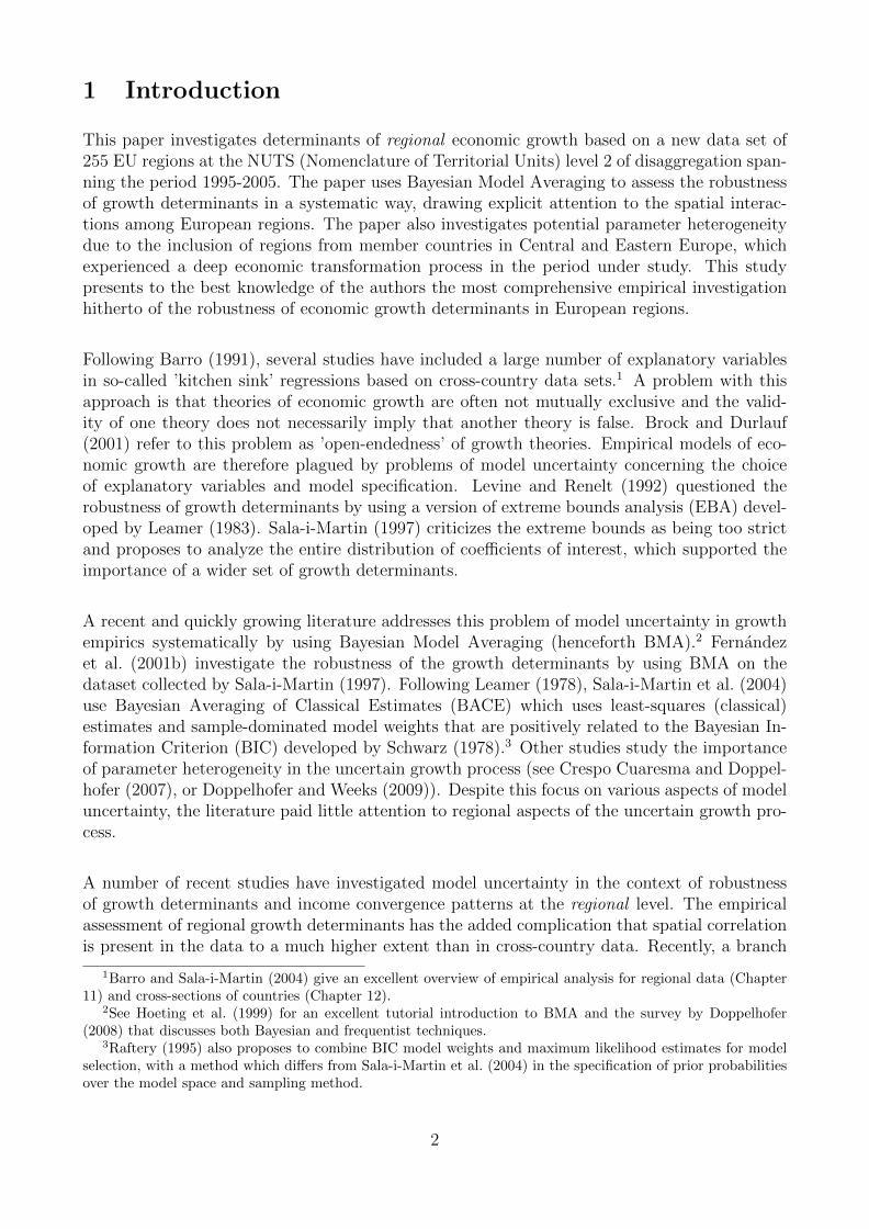
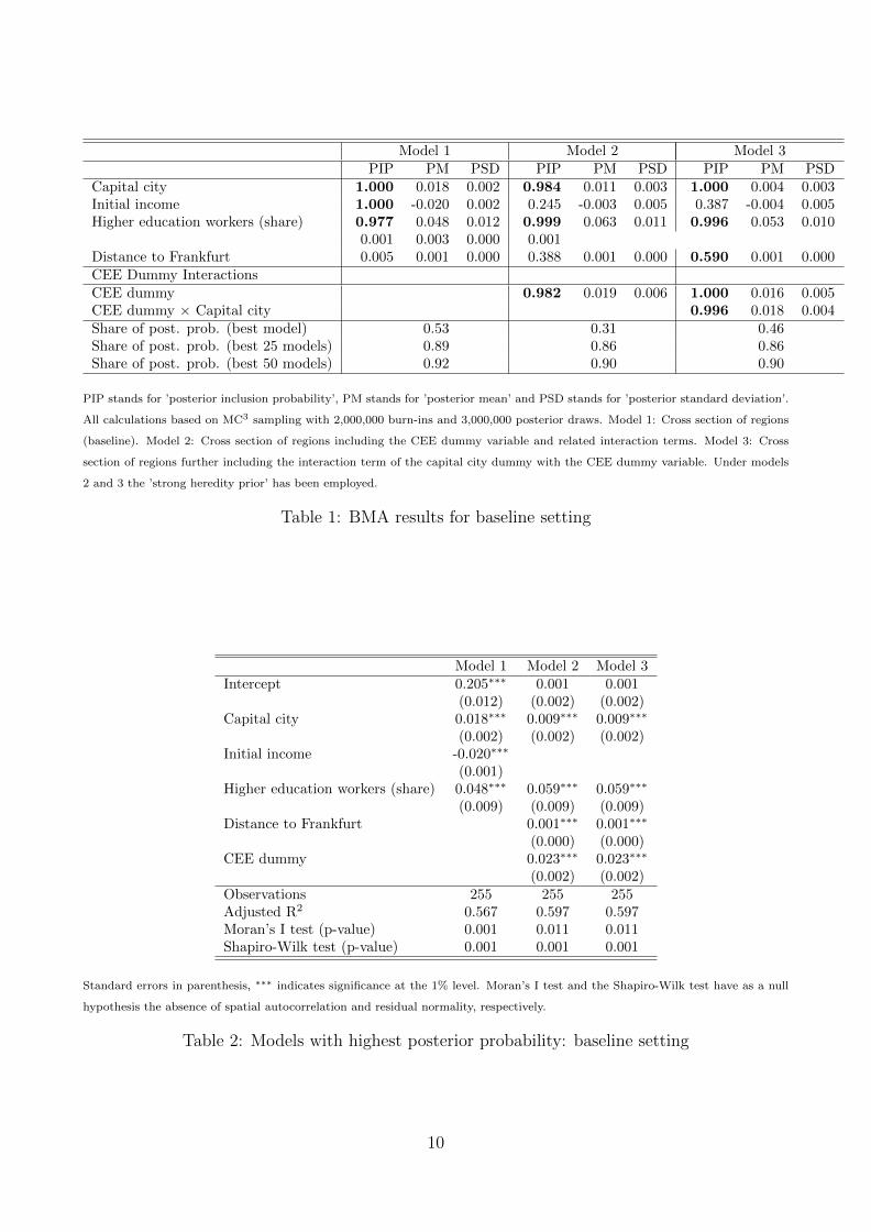
The top panel of Figure 1 illustrates the impact of explicitly modelling heterogeneity in the in-tercept across European regions. The left hand side of Figure 1 (top panel) shows the posterior

11

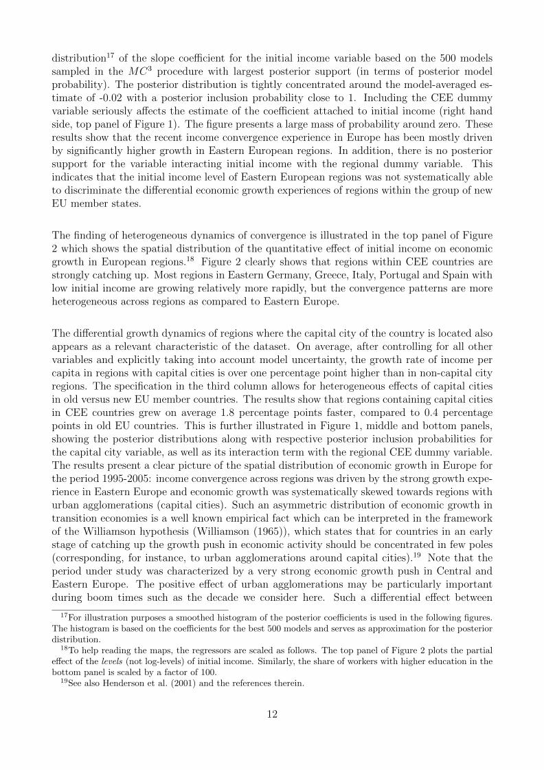
distribution17 of the slope coefficient for the initial income variable based on the 500 modelssampled in the MC3 procedure with largest posterior support (in terms of posterior modelprobability). The posterior distribution is tightly concentrated around the model-averaged es-timate of -0.02 with a posterior inclusion probability close to 1. Including the CEE dummyvariable seriously affects the estimate of the coefficient attached to initial income (right handside, top panel of Figure 1). The figure presents a large mass of probability around zero. Theseresults show that the recent income convergence experience in Europe has been mostly drivenby significantly higher growth in Eastern European regions. In addition, there is no posteriorsupport for the variable interacting initial income with the regional dummy variable. Thisindicates that the initial income level of Eastern European regions was not systematically ableto discriminate the differential economic growth experiences of regions within the group of newEU member states.

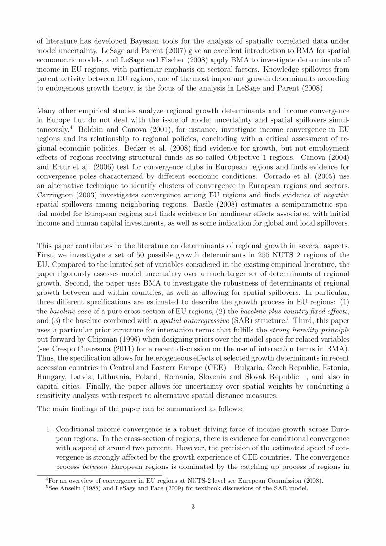
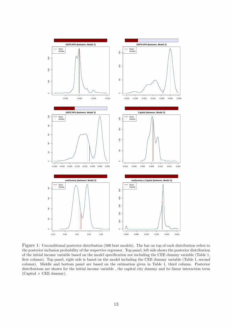
The finding of heterogeneous dynamics of convergence is illustrated in the top panel of Figure2 which shows the spatial distribution of the quantitative effect of initial income on economicgrowth in European regions.18 Figure 2 clearly shows that regions within CEE countries arestrongly catching up. Most regions in Eastern Germany, Greece, Italy, Portugal and Spain withlow initial income are growing relatively more rapidly, but the convergence patterns are moreheterogeneous across regions as compared to Eastern Europe.

The differential growth dynamics of regions where the capital city of the country is located alsoappears as a relevant characteristic of the dataset. On average, after controlling for all othervariables and explicitly taking into account model uncertainty, the growth rate of income percapita in regions with capital cities is over one percentage point higher than in non-capital cityregions. The specification in the third column allows for heterogeneous effects of capital citiesin old versus new EU member countries. The results show that regions containing capital citiesin CEE countries grew on average 1.8 percentage points faster, compared to 0.4 percentagepoints in old EU countries. This is further illustrated in Figure 1, middle and bottom panels,showing the posterior distributions along with respective posterior inclusion probabilities forthe capital city variable, as well as its interaction term with the regional CEE dummy variable.The results present a clear picture of the spatial distribution of economic growth in Europe forthe period 1995-2005: income convergence across regions was driven by the strong growth expe-rience in Eastern Europe and economic growth was systematically skewed towards regions withurban agglomerations (capital cities). Such an asymmetric distribution of economic growth intransition economies is a well known empirical fact which can be interpreted in the frameworkof the Williamson hypothesis (Williamson (1965)), which states that for countries in an earlystage of catching up the growth push in economic activity should be concentrated in few poles(corresponding, for instance, to urban agglomerations around capital cities).19 Note that theperiod under study was characterized by a very strong economic growth push in Central andEastern Europe. The positive effect of urban agglomerations may be particularly importantduring boom times such as the decade we consider here. Such a differential effect between

17For illustration purposes a smoothed histogram of the posterior coefficients is used in the following figures.The histogram is based on the coefficients for the best 500 models and serves as approximation for the posteriordistribution.

18To help reading the maps, the regressors are scaled as follows. The top panel of Figure 2 plots the partialeffect of the levels (not log-levels) of initial income. Similarly, the share of workers with higher education in thebottom panel is scaled by a factor of 100.

19See also Henderson et al. (2001) and the references therein.

12

−0.025 −0.020 −0.015 −0.010

010

020

030

0

GDPCAP0 (between, Model 1)

MeanMedian

−0.025 −0.020 −0.015 −0.010 −0.005 0.000 0.005

050

100

150

GDPCAP0 (between, Model 2)

MeanMedian

−0.030 −0.025 −0.020 −0.015 −0.010 −0.005 0.000 0.005

020

4060

8010

0

GDPCAP0 (between, Model 3)

MeanMedian

−0.010 −0.005 0.000 0.005 0.010 0.015 0.020

050

100

150

200

Capital (between, Model 3)

MeanMedian

−0.01 0.00 0.01 0.02 0.03

020

4060

80

ceeDummy (between, Model 3)

MeanMedian

0.000 0.005 0.010 0.015 0.020 0.025

010

020

030

040

050

0

ceeDummy.x.Capital (between, Model 3)

MeanMedian

Figure 1: Unconditional posterior distribution (500 best models). The bar on top of each distribution refers tothe posterior inclusion probability of the respective regressor. Top panel, left side shows the posterior distributionof the initial income variable based on the model specification not including the CEE dummy variable (Table 1,first column). Top panel, right side is based on the model including the CEE dummy variable (Table 1, secondcolumn). Middle and bottom panel are based on the estimation given in Table 1, third column. Posteriordistributions are shown for the initial income variable , the capital city dummy and its linear interaction term(Capital × CEE dummy).

13

under −1.15−1.15 − −1.02−1.02 − −0.86−0.86 − −0.62over −0.62

under 0.290.29 − 0.520.52 − 0.680.68 − 0.81over 0.81

Figure 2: Spatial distribution of the estimated effect due to income convergence and human capital accumula-tion for the cross section specification (Table 1, third column). Top panel shows the spatial distribution of thecoefficient on GDP per capita, the bottom panel the one for a human capital proxy.

14

Eastern and Western Europe further stresses the importance of modelling the regional growthprocess in Europe using data generating processes which allow for such heterogeneity.

The positive effect of human capital on economic growth is reflected in a robust positive pa-rameter estimate attached to the variable measuring the share of workers with higher (tertiary)education. The size of the model averaged estimate in the model with interactions (third set ofcolumns in Table 1) implies that on average a ten percent increase of the share of the workingage population with tertiary education is associated with a 0.5 percent higher growth rate ofGDP per capita. Compared to the sample average growth rate of 2.2 percent for all regionsin the sample, the effect is quantitatively substantial. The bottom panel of Figure 2 showsthe regional distribution of mean estimates of the effect of the human capital variable acrossregions. The strongest effects of human capital on economic growth are located in the centralregions in Germany, Benelux countries and Scandinavia as well as Southern regions in the UK.When comparing economic effects of education (and other growth determinants), the modelassumes that EU regions have similar access to technologies (Vandenbussche et al. (2006)). Inprinciple, some of the variation in the shares of workers with higher education - measured asthose who completed tertiary education - might be attributed to the fact that education sys-tems vary across countries. The next subsection shows that human capital remains importantin explaining growth differences also in the specification including country-fixed effects, whereheterogeneity in national education systems is controlled for.

As explained above and reported in Table 1, when parameter heterogeneity between old and newmember states is allowed for, the evidence concerning robust convergence decreases, reflectedalso in the mean of the posterior distribution of the coefficient associated with initial income.The results of the most general specification setting therefore confirm the importance of humancapital formation as an engine of economic growth among European regions and the over-proportional growth performance of regions containing the capital city. On the other hand, thestrong growth performance of emerging economies in Central Eastern Europe appears as themain responsible for the existence of robust income convergence across regions in Europe andfor the evidence of convergence poles at the regional level in Europe in the period 1995-2005.

3.2 Regional growth determinants within countries

The results shown in Table 3 are based on BMA with models containing country fixed effectsthat concentrate on regional differences of growth and its determinants within countries. Thespecification can therefore account for unobserved time-invariant country specific characteristicsthat could affect the process of economic growth. Note that in this specification the dynamicsof income convergence, associated with the coefficient of initial income per capita, should beinterpreted as taking place in regions within a country towards a country-specific steady state20.Comparing the results in Tables 1 and 3, CEE regions contributed mostly to the regional incomeconvergence process between countries, whereas income convergence within countries is mostlya characteristic of old EU member states. This evidence is in line with the trends in income

20Note that the CEE dummy variable is not identified when including fixed effects. We consequently excludethe CEE dummy for the estimations provided in Table 3 and do not employ the strong heredity prior for thelinear interaction terms. Furthermore note that the capital city dummy does not suffer from identificationproblems since the case that all regions of a country (when there is more than one) contain national capitalcities is ruled out by definition.

15

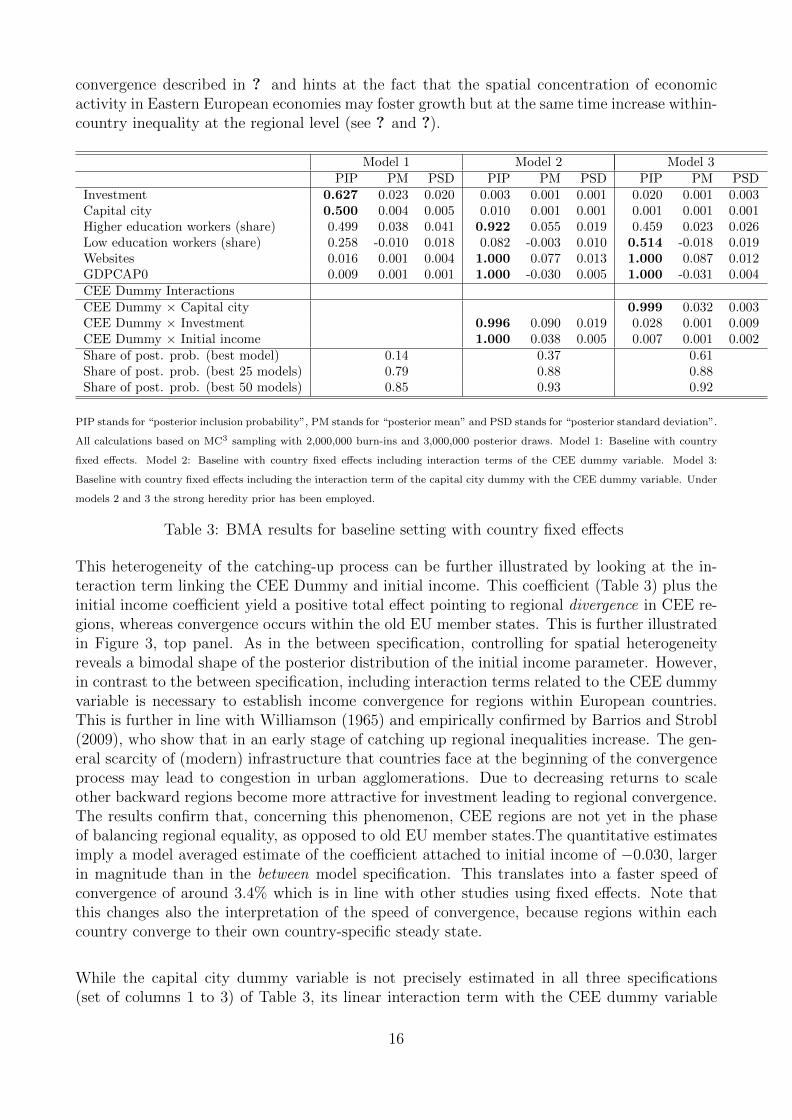
convergence described in ? and hints at the fact that the spatial concentration of economicactivity in Eastern European economies may foster growth but at the same time increase within-country inequality at the regional level (see ? and ?).

Model 1 Model 2 Model 3PIP PM PSD PIP PM PSD PIP PM PSD

Investment 0.627 0.023 0.020 0.003 0.001 0.001 0.020 0.001 0.003Capital city 0.500 0.004 0.005 0.010 0.001 0.001 0.001 0.001 0.001Higher education workers (share) 0.499 0.038 0.041 0.922 0.055 0.019 0.459 0.023 0.026Low education workers (share) 0.258 -0.010 0.018 0.082 -0.003 0.010 0.514 -0.018 0.019Websites 0.016 0.001 0.004 1.000 0.077 0.013 1.000 0.087 0.012GDPCAP0 0.009 0.001 0.001 1.000 -0.030 0.005 1.000 -0.031 0.004CEE Dummy InteractionsCEE Dummy × Capital city 0.999 0.032 0.003CEE Dummy × Investment 0.996 0.090 0.019 0.028 0.001 0.009CEE Dummy × Initial income 1.000 0.038 0.005 0.007 0.001 0.002Share of post. prob. (best model) 0.14 0.37 0.61Share of post. prob. (best 25 models) 0.79 0.88 0.88Share of post. prob. (best 50 models) 0.85 0.93 0.92

PIP stands for “posterior inclusion probability”, PM stands for “posterior mean” and PSD stands for “posterior standard deviation”.

All calculations based on MC3 sampling with 2,000,000 burn-ins and 3,000,000 posterior draws. Model 1: Baseline with country

fixed effects. Model 2: Baseline with country fixed effects including interaction terms of the CEE dummy variable. Model 3:

Baseline with country fixed effects including the interaction term of the capital city dummy with the CEE dummy variable. Under

models 2 and 3 the strong heredity prior has been employed.

Table 3: BMA results for baseline setting with country fixed effects

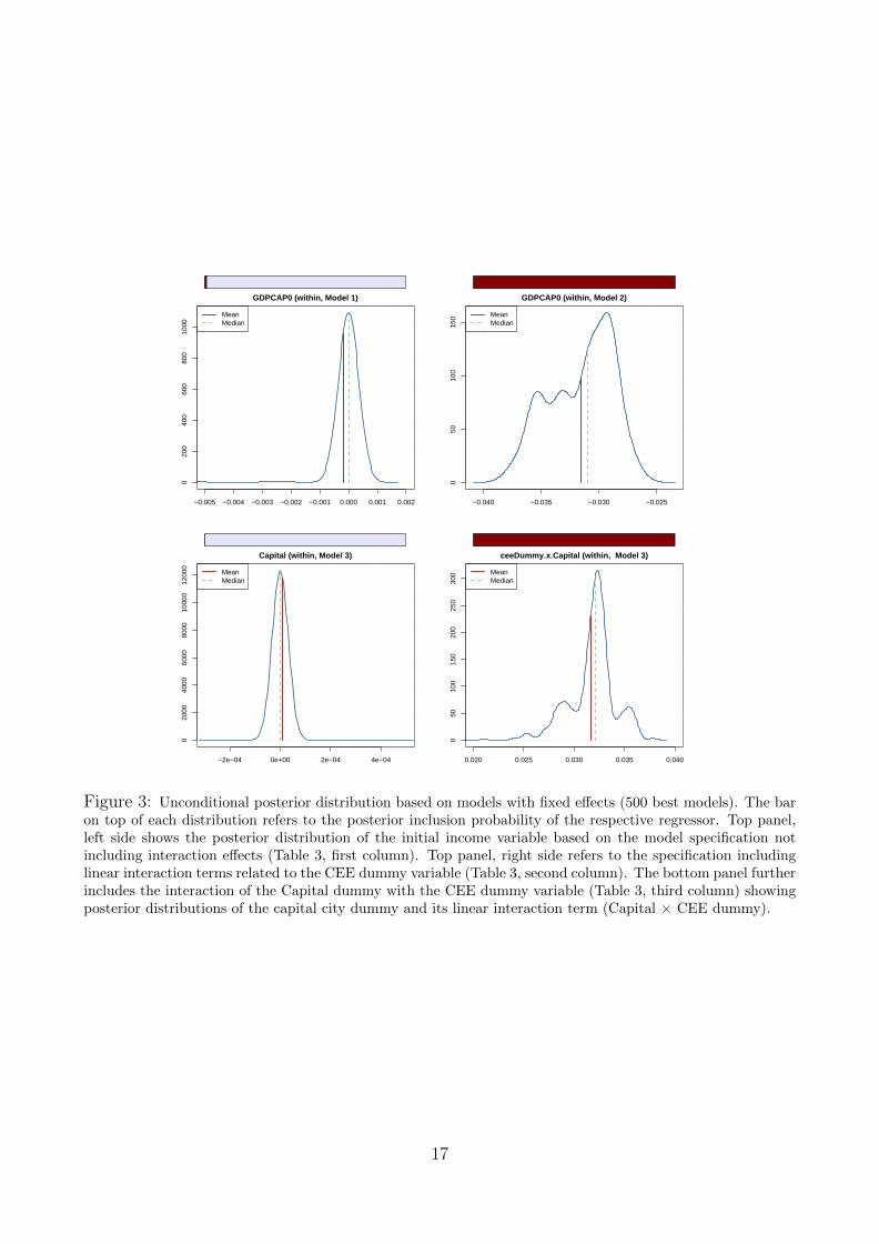
This heterogeneity of the catching-up process can be further illustrated by looking at the in-teraction term linking the CEE Dummy and initial income. This coefficient (Table 3) plus theinitial income coefficient yield a positive total effect pointing to regional divergence in CEE re-gions, whereas convergence occurs within the old EU member states. This is further illustratedin Figure 3, top panel. As in the between specification, controlling for spatial heterogeneityreveals a bimodal shape of the posterior distribution of the initial income parameter. However,in contrast to the between specification, including interaction terms related to the CEE dummyvariable is necessary to establish income convergence for regions within European countries.This is further in line with Williamson (1965) and empirically confirmed by Barrios and Strobl(2009), who show that in an early stage of catching up regional inequalities increase. The gen-eral scarcity of (modern) infrastructure that countries face at the beginning of the convergenceprocess may lead to congestion in urban agglomerations. Due to decreasing returns to scaleother backward regions become more attractive for investment leading to regional convergence.The results confirm that, concerning this phenomenon, CEE regions are not yet in the phaseof balancing regional equality, as opposed to old EU member states.The quantitative estimatesimply a model averaged estimate of the coefficient attached to initial income of −0.030, largerin magnitude than in the between model specification. This translates into a faster speed ofconvergence of around 3.4% which is in line with other studies using fixed effects. Note thatthis changes also the interpretation of the speed of convergence, because regions within eachcountry converge to their own country-specific steady state.

While the capital city dummy variable is not precisely estimated in all three specifications(set of columns 1 to 3) of Table 3, its linear interaction term with the CEE dummy variable

16

−0.005 −0.004 −0.003 −0.002 −0.001 0.000 0.001 0.002

020

040

060

080

010

00

GDPCAP0 (within, Model 1)

MeanMedian

−0.040 −0.035 −0.030 −0.025

050

100

150

GDPCAP0 (within, Model 2)

MeanMedian

−2e−04 0e+00 2e−04 4e−04

020

0040

0060

0080

0010

000

1200

0

Capital (within, Model 3)

MeanMedian

0.020 0.025 0.030 0.035 0.040

050

100

150

200

250

300

ceeDummy.x.Capital (within, Model 3)

MeanMedian

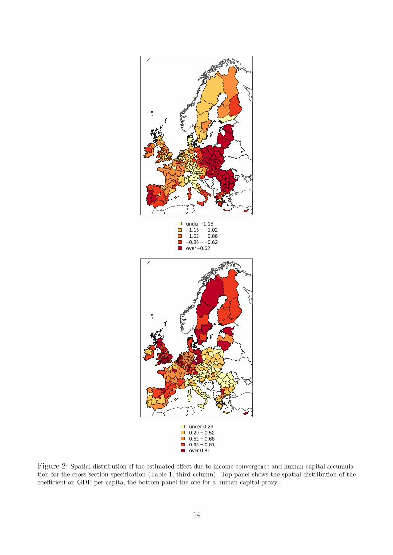
Figure 3: Unconditional posterior distribution based on models with fixed effects (500 best models). The baron top of each distribution refers to the posterior inclusion probability of the respective regressor. Top panel,left side shows the posterior distribution of the initial income variable based on the model specification notincluding interaction effects (Table 3, first column). Top panel, right side refers to the specification includinglinear interaction terms related to the CEE dummy variable (Table 3, second column). The bottom panel furtherincludes the interaction of the Capital dummy with the CEE dummy variable (Table 3, third column) showingposterior distributions of the capital city dummy and its linear interaction term (Capital × CEE dummy).

17

receives a high posterior inclusion probability in the third specification. This implies - as inthe between specification - that regions hosting a capital city that are further located in CEEreceive an additional growth bonus. Figure 3 corroborates our findings: The top panel, leftside, shows the posterior distribution of the parameter for initial income. After controllingfor spatial heterogeneity (in terms of East / West-specific parameters) by including linearinteraction terms related to the CEE dummy variable income convergence appears robust inthe data: The corresponding graph in Figure 3, top panel, right side shows a bimodal posteriordistribution with both mean and median negative indicating income convergence taking place.The bottom panel, left and right side shows the posterior distribution of the parameters for thecapital city as well as the corresponding linear interaction term with the CEE dummy variable.The distribution illustrates that CEE regions with a capital city tend to perform relativelybetter than other regions, with an additional and sizable bonus implied by the right shift of thedistribution shown at the bottom right panel of Figure 3.

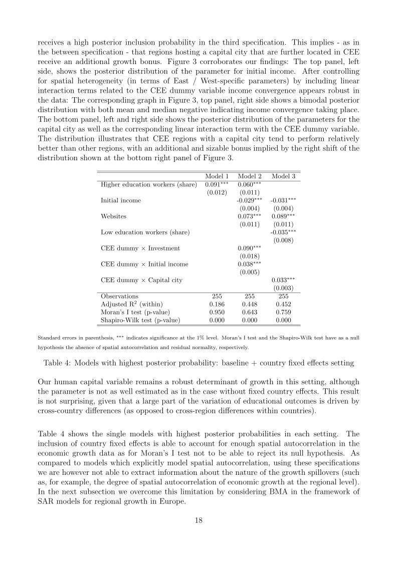
Model 1 Model 2 Model 3Higher education workers (share) 0.091∗∗∗ 0.060∗∗∗

(0.012) (0.011)Initial income -0.029∗∗∗ -0.031∗∗∗

(0.004) (0.004)Websites 0.073∗∗∗ 0.089∗∗∗

(0.011) (0.011)Low education workers (share) -0.035∗∗∗

(0.008)CEE dummy × Investment 0.090∗∗∗

(0.018)CEE dummy × Initial income 0.038∗∗∗

(0.005)CEE dummy × Capital city 0.033∗∗∗

(0.003)Observations 255 255 255Adjusted R2 (within) 0.186 0.448 0.452Moran’s I test (p-value) 0.950 0.643 0.759Shapiro-Wilk test (p-value) 0.000 0.000 0.000

Standard errors in parenthesis, ∗∗∗ indicates significance at the 1% level. Moran’s I test and the Shapiro-Wilk test have as a null

hypothesis the absence of spatial autocorrelation and residual normality, respectively.

Table 4: Models with highest posterior probability: baseline + country fixed effects setting

Our human capital variable remains a robust determinant of growth in this setting, althoughthe parameter is not as well estimated as in the case without fixed country effects. This resultis not surprising, given that a large part of the variation of educational outcomes is driven bycross-country differences (as opposed to cross-region differences within countries).

Table 4 shows the single models with highest posterior probabilities in each setting. Theinclusion of country fixed effects is able to account for enough spatial autocorrelation in theeconomic growth data as for Moran’s I test not to be able to reject its null hypothesis. Ascompared to models which explicitly model spatial autocorrelation, using these specificationswe are however not able to extract information about the nature of the growth spillovers (suchas, for example, the degree of spatial autocorrelation of economic growth at the regional level).In the next subsection we overcome this limitation by considering BMA in the framework ofSAR models for regional growth in Europe.

18

3.3 Growth spillovers in Europe - Robust growth determinants un-der spatial autocorrelation

The model with country fixed effects presented above assesses the issue of spatial correlation ofincome growth by assuming a country-specific intercept, common to all regions within a nation,in the economic growth process. To the extent that country borders are not a large obstaclein the growth process of EU regions, using membership of regions in countries may not be thebest way of modeling spatial relationships in the dataset. Alternatively, actual geographicaldistance can be used in the framework of SAR models such as those presented above to relatethe growth process of different regions.

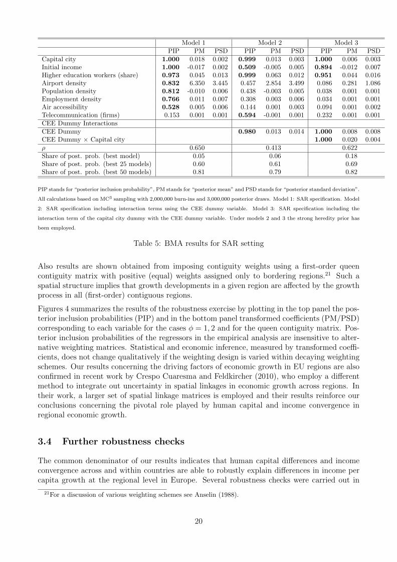
Table 5 presents the results of the BMA exercise for the class of SAR models, using inversedistances to construct the matrix of spatial weights W. The number of robust variables whenspatial autocorrelation is explicitly modeled is higher than in any other setting. The modelaveraged estimate of the spatial autocorrelation parameter ρ reveals positive spatial autocor-relation in income growth across European regions. The results obtained in the specificationswithout spatial autocorrelation are still present in the estimates from the SAR specification:regions with capital cities, regions with lower income and regions with a relatively educatedlabor force tend to present higher growth rates of income. Strikingly, initial income appearsalso as robust in the preferred specification that allows for capital city effects together withregional heterogeneity captured by the CEE dummy variable. This finding contrasts the resultsof the linear model and underscores the importance of ’correct’ modeling of spatial correlation.

The posterior estimates using the SAR specification are close to the ones using the linear regres-sion model. In particular, regions containing capital cities in CEE countries grew on average 2percentage points faster, compared to 0.6 percentage points in old EU countries. Furthermore,a ten percent increase of the share of workers with higher education is associated with a 0.4percent higher growth rate of GDP per capita, a finding that is very close to that reportedin Section 3.1. As for the specifications above, we also present the models with the highestposterior probability, which are shown in Table 6. For the case of SAR specifications, the pos-terior model probability appears more spread across models than in the cases without spatialautoregressive terms, and there appears to be a large degree of variability in spatial autocorre-lation estimates (see the differences in estimates of ρ in Table 6. Thus, a rigorous assessment ofmodel uncertainty is important when considering spatial models for regional economic growthin Europe.

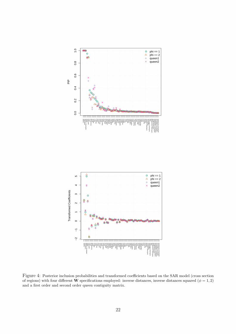
Since economic theory does not offer much guidance concerning a particular choice of spatialweighting matrix W, the paper finally assesses the robustness of the findings with respect tothe choice of the spatial link matrix. While the inverse distance matrix used hitherto is arecurrent choice in spatial econometric applications, it can be thought of as a special case of amore general weighting matrix W(φ) with a characteristic element

[W]ij = [dij]−φ, (5)

where dij is the distance between regions i and j and the parameter φ embodies the sensitivityof weights to distance, and thus the decay of the weighting scheme. The benchmark value(φ = 1) implies that weights are an inverse function of distance, while higher values of φ lead toa stronger decay of weights with distance. To test the sensitivity of results, the BMA exerciseis repeated for parameter value φ = 2, which implies a faster decay of weights with distance.

19

Model 1 Model 2 Model 3PIP PM PSD PIP PM PSD PIP PM PSD

Capital city 1.000 0.018 0.002 0.999 0.013 0.003 1.000 0.006 0.003Initial income 1.000 -0.017 0.002 0.509 -0.005 0.005 0.894 -0.012 0.007Higher education workers (share) 0.973 0.045 0.013 0.999 0.063 0.012 0.951 0.044 0.016Airport density 0.832 6.350 3.445 0.457 2.854 3.499 0.086 0.281 1.086Population density 0.812 -0.010 0.006 0.438 -0.003 0.005 0.038 0.001 0.001Employment density 0.766 0.011 0.007 0.308 0.003 0.006 0.034 0.001 0.001Air accessibility 0.528 0.005 0.006 0.144 0.001 0.003 0.094 0.001 0.002Telecommunication (firms) 0.153 0.001 0.001 0.594 -0.001 0.001 0.232 0.001 0.001CEE Dummy InteractionsCEE Dummy 0.980 0.013 0.014 1.000 0.008 0.008CEE Dummy × Capital city 1.000 0.020 0.004ρ 0.650 0.413 0.622Share of post. prob. (best model) 0.05 0.06 0.18Share of post. prob. (best 25 models) 0.60 0.61 0.69Share of post. prob. (best 50 models) 0.81 0.79 0.82

PIP stands for “posterior inclusion probability”, PM stands for “posterior mean” and PSD stands for “posterior standard deviation”.

All calculations based on MC3 sampling with 2,000,000 burn-ins and 3,000,000 posterior draws. Model 1: SAR specification. Model

2: SAR specification including interaction terms using the CEE dummy variable. Model 3: SAR specification including the

interaction term of the capital city dummy with the CEE dummy variable. Under models 2 and 3 the strong heredity prior has

been employed.

Table 5: BMA results for SAR setting

Also results are shown obtained from imposing contiguity weights using a first-order queencontiguity matrix with positive (equal) weights assigned only to bordering regions.21 Such aspatial structure implies that growth developments in a given region are affected by the growthprocess in all (first-order) contiguous regions.

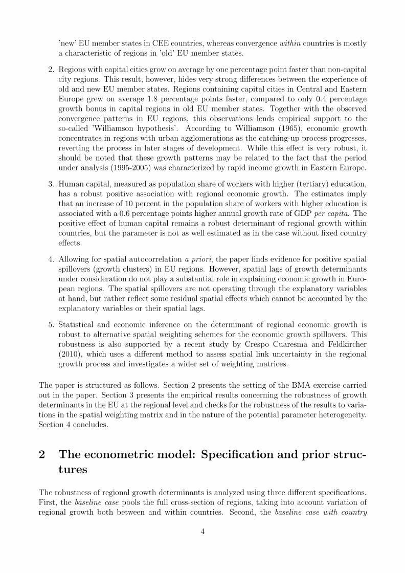
Figures 4 summarizes the results of the robustness exercise by plotting in the top panel the pos-terior inclusion probabilities (PIP) and in the bottom panel transformed coefficients (PM/PSD)corresponding to each variable for the cases φ = 1, 2 and for the queen contiguity matrix. Pos-terior inclusion probabilities of the regressors in the empirical analysis are insensitive to alter-native weighting matrices. Statistical and economic inference, measured by transformed coeffi-cients, does not change qualitatively if the weighting design is varied within decaying weightingschemes. Our results concerning the driving factors of economic growth in EU regions are alsoconfirmed in recent work by Crespo Cuaresma and Feldkircher (2010), who employ a differentmethod to integrate out uncertainty in spatial linkages in economic growth across regions. Intheir work, a larger set of spatial linkage matrices is employed and their results reinforce ourconclusions concerning the pivotal role played by human capital and income convergence inregional economic growth.

3.4 Further robustness checks

The common denominator of our results indicates that human capital differences and incomeconvergence across and within countries are able to robustly explain differences in income percapita growth at the regional level in Europe. Several robustness checks were carried out in

21For a discussion of various weighting schemes see Anselin (1988).

20

Model 1 Model 2 Model 3Intercept 0.1640∗∗∗ 0.0224∗∗ -0.0228

(0.0229) (0.0104) (0.0160)Air accessibility 0.0129∗∗∗

(0.0029)Road accessibility -0.0139∗∗∗ -0.0031 -0.0041∗∗∗

(0.0025) (0.0023) (0.0013)Capital city 0.0152∗∗∗ 0.0112∗∗∗ 0.0106∗∗∗

(0.0019) (0.0019) (0.0018)Initial income -0.0126∗∗∗

(0.0021)Coastal -0.0024∗

(0.0013)Pentagon 0.0071∗∗∗

(0.0020)Low education workers (share) -0.0308∗∗∗ -0.0113∗

(0.0047) (0.0059)Telecommunications (firms) -0.0027∗∗∗ -0.0025∗∗∗ -0.0026∗∗∗

(0.0007) (0.0006) (0.0005)Distance to Frankfurt 0.0001

(0.0001)Higher education workers (share) 0.0555∗∗∗ 0.0745∗∗∗

(0.0112) (0.0091)Activity rate (higher education) 0.0458∗∗

(0.0179)CEE dummy 0.0173∗∗∗ 0.0185∗∗∗

(0.0024) (0.0020)ρ -0.013 0.035 0.104

(0.316) (0.349) (0.324)Observations 255 255 255Shapiro-Wilk test (p-value) 0.010 0.000 0.000

Standard errors in parenthesis, ∗∗∗(∗∗)[∗] indicates significance at the 1% (5%)[10%] level. The Shapiro-Wilk test has as a null

hypothesis residual normality.

Table 6: Models with highest posterior probability: SAR setting

21

●●●

●

●

●

●●

●

●●

●

●●●●●●●●●●●●●●●●●●●●●●●●●●●●●●●●●●●●●●●●●●●●●●●●0.

00.

20.

40.

60.

81.

0

PIP

● phi == 1phi == 2queen1queen2

Cap

ital

ceeD

umm

yce

eDum

my.

x.C

apita

lS

hSH

GD

PC

AP

0IN

TF

Acc

essR

oad

gPO

PA

irpor

tsT

ELF

Dis

tde7

1U

RL0

shG

FC

FA

cces

sAir

AR

H0

Airp

ortD

ens

UR

T0

Sea

port

sR

egC

oast

Con

nect

Air

Reg

Obj

1P

aten

tHT

Reg

Pen

t27

ER

EH

0U

RH

0P

aten

tICT

PO

PD

EN

S0

ShA

B0

Dis

tCap

EM

PD

EN

S0

ER

ET

0R

oadD

ens

ER

EL0

ShL

LLS

hSL

Pat

entT

ShC

E0

Pat

entB

IOP

aten

tShH

TA

RT

0P

aten

tShI

CT

Con

nect

Sea

TE

LHH

RS

Tco

reO

UT

DE

NS

0P

aten

tShB

IOA

RL0

Tem

pR

ailD

ens

Haz

ard

ceeD

umm

y.x.

shG

FC

FR

egB

oard

erce

eDum

my.

x.G

DP

CA

P0

Set

tlce

eDum

my.

x.A

cces

sRoa

dce

eDum

my.

x.gP

OP

ceeD

umm

y.x.

PO

PD

EN

S0

ceeD

umm

y.x.

EM

PD

EN

S0

ceeD

umm

y.x.

HR

ST

core

ceeD

umm

y.x.

OU

TD

EN

S0

●

●

●

●

●

●

●

●●

●

●

●

●●●●

●

●

●●

●●●●●●

●

●

●

●●●●●●●●●●

●●●●●●●●●●●

●●●●●●●●●●

−2

−1

01

23

45

Tra

nsfo

rmed

Coe

ffici

ents

● phi == 1phi == 2queen1queen2

Cap

ital

ceeD

umm

yce

eDum

my.

x.C

apita

lS

hSH

GD

PC

AP

0IN

TF

Acc

essR

oad

gPO

PA

irpor

tsT

ELF

Dis

tde7

1U

RL0

shG

FC

FA

cces

sAir

AR

H0

Airp

ortD

ens

UR

T0

Sea

port

sR

egC

oast

Con

nect

Air

Reg

Obj

1P

aten

tHT

Reg

Pen

t27

ER

EH

0U

RH

0P

aten

tICT

PO

PD

EN

S0

ShA

B0

Dis

tCap

EM

PD

EN

S0

ER

ET

0R

oadD

ens

ER

EL0

ShL

LLS

hSL

Pat

entT

ShC

E0

Pat

entB

IOP

aten

tShH

TA

RT

0P

aten

tShI

CT

Con

nect

Sea

TE

LHH

RS

Tco

reO

UT

DE

NS

0P

aten

tShB

IOA

RL0

Tem

pR

ailD

ens

Haz

ard

ceeD

umm

y.x.

shG

FC

FR

egB

oard

erce

eDum

my.

x.G

DP

CA

P0

Set

tlce

eDum

my.

x.A

cces

sRoa

dce

eDum

my.

x.gP

OP

ceeD

umm

y.x.

PO

PD

EN

S0

ceeD

umm

y.x.

EM

PD

EN

S0

ceeD

umm

y.x.

HR

ST

core

ceeD

umm

y.x.

OU

TD

EN

S0

Figure 4: Posterior inclusion probabilities and transformed coefficients based on the SAR model (cross sectionof regions) with four different W specifications employed: inverse distances, inverse distances squared (φ = 1, 2)and a first order and second order queen contiguity matrix.

22

order to ensure that our results do not depend on the particular setting put forward in this study.

To further investigate the transmission channels of growth spillovers, we allowed spatial spilloversto occur via the explanatory variables, as in the unrestricted Spatial Durbin model. Thus, thebenchmark setting and the benchmark with country fixed effects setting were re-estimated withan enlarged set of potential growth determinants by introducing spatial lags of the potentialcovariates. The results presented above are left unchanged under the enlarged set of variables.22

The spatially lagged explanatory variables do not appear as robust determinants of regionalgrowth. This suggests that the positive correlation found from the SAR specification is drivenby other factors not captured by the variables under consideration.

A further criticism that could be exercised on our analysis is related to the fact that manyof our covariates are highly correlated. This could lead to multicollinearity problems in sin-gle specifications which would lead to inflated estimates of the uncertainty surrounding singleparameter estimates. Some solutions to deal with correlated regressors in the framework ofBMA have been proposed in the literature. In particular, Durlauf et al. (2008) propose to use adilution prior of the type put forward in George (2007). They propose to use the determinantof the correlation matrix of regressors multiplicatively in the prior model probability. Thisdilution prior punishes models that contain highly collinear variables. The determinant of anuncorrelated set of regressors will be close to 1, while highly correlated regressors will result ina determinant close to 0. We repeated our analysis using this prior specification and the resultsdid not change qualitatively as compared to those presented above. Our results appear thusalso robust to the explicit assessment of potential multicollinearity among covariates.

4 Conclusions

This paper analyzes the nature of robust determinants of economic growth in EU regions inthe presence of model uncertainty using model averaging techniques. The paper contains someimportant novelties compared to previous studies on the topic. On the one hand, the paperuses the most comprehensive dataset existing (to the knowledge of the authors) on potentialdeterminants of economic growth in European regions. On the other hand, the paper appliesthe most recent Bayesian Model Averaging techniques to assess the issue of robustness of growthdeterminants. In particular, the empirical estimation framework allows for spatial autoregres-sive structures, hyperpriors on model size to robustify the prior choice on the model spaceand introduce a new methodology to treat the issue of subsample parameter heterogeneity viainteraction terms.

The results imply that conditional income convergence appears to be a robust driving forceof income growth across European regions. Between EU regions of different countries, thiscatching-up process has been fuelled by the growth experience in Eastern Europe. Convergencewithin countries, on the other hand, is concentrated in Western European economies. Regionswith capital cities exhibit a significantly higher growth performance than other regions (be-

22Detailed BMA results for the setting with an enlarged set of covariates are available upon request from theauthors.

23

tween specification) and this asymmetry is particularly sizable in Eastern European economies(between and within specification), which lends further support to the differential regional dy-namics proposed by the Williamson hypothesis in the catching-up process. The importance ofeducation as a growth engine appears also clearly in the data, which show that a higher shareof educated workers in the labor force is positively associated with regional economic growth.The paper also finds evidence for positive spatial economic growth spillovers among EU regions.

The BMA method used in the paper allows for further generalizations which can be very fruitfulas future research avenues: (a) exploiting alternative spatial weights matrices, as is done inCrespo Cuaresma and Feldkircher (2010), can help us further understand the nature of economicgrowth spillovers in Europe; (b) combining the methods proposed here with BMA settings whichallow for nonlinear data generating processes (see e.g. Crespo Cuaresma and Doppelhofer(2007)) could shed light on the heterogeneity of growth processes within the European Unionbeyond the East/West differences highlighted in this study; (c) the availability of further datamay allow for the use of instrumental variable methods in the framework of BMA to explicitlyassess potential endogeneity in the link between economic growth and its determinants.

24

References

Anselin, L. (1988). Spatial Econometrics: Methods and Models. Kluwer Academic Publishers.

Barrios, S. and Strobl, E. (2009). The dynamics of regional inequalities. Regional Science andUrban Economics, 39:5:575–591.

Barro, R. J. (1991). Economic Growth in a Cross Section of Countries. The Quarterly Journalof Economics, 106, No. 2:407–443.

Barro, R. J. and Sala-i-Martin, X. (2004). Economic Growth. MIT Press.

Basile, R. (2008). Regional Economic Growth in Europe: A Semiparametric Spatial DependenceApproach. Papers in Regional Science, 87:527–544.

Becker, S. O., von Ehrlich, M., Egger, P., and Fenge, R. (2008). Going NUTS: The Effect ofEU Structural Funds on Regional Performance. Working Paper 2495, CESifo.

Boldrin, M. and Canova, F. (2001). Inequality and Convergence in Europe’s Regions: Recon-sidering European Regional Policies. Economic Policy, 16:205–253.

Brock, W. and Durlauf, S. (2001). Growth Empirics and Reality. World Bank EconomicReview, 15:229–272.

Brown, P., Vannucci, M., and Fearn, T. (1998). Multivariate Bayesian Variable Selection andPrediction. Journal of the Royal Statistical Society B, 60:627–641.

Canova, F. (2004). Testing for Convergence Clubs in Income Per Capita: A Predictive DensityApproach. International Economic Review, 45:49–77.

Carrington, A. (2003). A Divided Europe? Regional Convergence and Neighborhood SpilloverEffects. Kyklos, 56:381–393.

Chipman, H. (1996). Bayesian Variable Selection with Related Predictors. Canadian Journalof Statistics, 24:17–36.

Corrado, L., Martin, R., and Weeks, M. (2005). Identifying and Interpreting Regional Conver-gence Clusters across Europe. Economic Journal, 115:C133–C160.

Crespo Cuaresma, J. (2011). How different is Africa? A comment on Masanjala and Papageor-giou (2008). Journal of Applied Econometrics, forthcoming.

Crespo Cuaresma, J. and Doppelhofer, G. (2007). Nonlinearities in Cross-Country Growth Re-gressions: A Bayesian Averaging of Thresholds (BAT) Approach. Journal of Macroeconomics,29:541–554.

Crespo Cuaresma, J. and Feldkircher, M. (2010). Spatial Filtering, Model Uncertainty andthe Speed of Income Convergence in Europe. Working Papers 160, Working Papers 160,Oesterreichische Nationalbank (Austrian Central Bank).

Doppelhofer, G. (2008). The New Palgrave Dictionary of Economics. Second Edition, chapterModel Averaging. Palgrave Macmillan.

25

Doppelhofer, G. and Weeks, M. (2009). Jointness of Growth Determinants. Journal of AppliedEconometrics, 24(2):209–244.

Doppelhofer, G. and Weeks, M. (2011). Robust Growth Determinants. CESifo Working Paper,No. 3354.

Durlauf, S., Kourtellos, A., and Tan, C. (2008). Are Any Growth Theories Robust? EconomicJournal, 118:329–346.

Eicher, T. S., Papageorgiou, C., and Raftery, A. E. (2011). Default priors and predictiveperformance in bayesian model averaging, with application to growth determinants. Journalof Applied Econometrics, 26(1):30–55.

Ertur, C. and Koch, W. (2006). Regional Disparities in the European Union and the Enlarge-ment Process: An Exploratory Spatial Data Analysis, 1995-2000. Annals of Regional Science,40(4):723–765.

Ertur, C., Le Gallo, J., and Baumont, C. (2006). The European Regional Convergence Process,1980-1995: Do Spatial Regimes and Spatial Dependence Matter? International RegionalScience Review, 29:3–34.

European Commission (2008). Convergence of eu regions: Measures and evolution. WorkingPaper 01, Directorate General for Regional Policy.

Fernandez, C., Ley, E., and Steel, M. F. (2001a). Benchmark Priors for Bayesian Model Aver-aging. Journal of Econometrics, 100:381–427.

Fernandez, C., Ley, E., and Steel, M. F. (2001b). Model Uncertainty in Cross-Country GrowthRegressions. Journal of Applied Econometrics, 16:563–576.

Fischer, M. and Stirbock, C. (2006). Pan-European Regional Income Growth and Club-Convergence. Insights from a Spatial Econometric Perspective. Annals of Regional Science,40(3):1–29.

Foster, D. P. and George, E. I. (1994). The Risk Inflation Criterion for Multiple Regression.The Annals of Statistics, 22:1947–1975.

Frisch, R. and Waugh, F. V. (1933). Partial Time Regressions as Compared with IndividualTrends. Econometrica, 1 (4):387–401.

George, E. (2007). Discussion of Bayesian Model Averaging and Model Search Strategies byM.A. Clyde. Bayesian Statistics, pages 157–77.

Hauk, W. and Wacziarg, R. (2009). A Monte Carlo study of growth regressions. Journal ofEconomic Growth, 14:103–147.

Henderson, J. V., Shalizi, Z., and Venables, A. J. (2001). Geography and development. Journalof Economic Geography, Oxford University Press, vol. 1(1):81–105.

Hoeting, J. A., Madigan, D., Raftery, A. E., and Volinsky, C. T. (1999). Bayesian ModelAveraging: A Tutorial. Statistical Science, 14, No. 4:382–417.

Kass, R. and Raftery, A. (1995). Bayes Factors. Journal of the American Statistical Association,90:773–795.

26

Koop, G. (2003). Bayesian Econometrics. John Wiley & Sons.

Leamer, E. (1978). Specification Searches. John Wiley and Sons, New York.

Leamer, E. (1983). Let’s take the Con out of Econometrics. American Economic Review,73:31–43.

LeSage, J. and Pace, R. (2009). Introduction to Spatial Econometrics. Chapman & Hall, CRC.

LeSage, J. P. and Fischer, M. (2008). Spatial Growth Regressions, Model Specification, Esti-mation, and Interpretation. Spatial Economic Analysis, 3:275–304.

LeSage, J. P. and Parent, O. (2007). Bayesian Model Averaging for Spatial Econometric Models.Geographical Analysis, 39:3:241–267.

LeSage, J. P. and Parent, O. (2008). Using the Variance Structure of the Conditional SpatialSpecifcation to Model Knowledge Spillovers. Journal of Applied Econometrics, 23:235–256.

Levine, R. and Renelt, D. (1992). A Sensitivity Analysis of Cross-Country Growth Regressions.American Economic Review, 82:942–963.

Ley, E. and Steel, M. F. (2009). On the Effect of Prior Assumptions in Bayesian Model Averag-ing with Applications to Growth Regressions. Journal of Applied Econometrics, 24:4:651–674.

Madigan, D. and York, J. (1995). Bayesian graphical models for discrete data. InternationalStatistical Review, 63.:215–232.

Masanjala, W. H. and Papageorgiou, C. (2008). Rough and Lonely Road to Prosperity: AReexamination of the Sources of Growth in Africa Using Bayesian Model Averaging. Journalof Applied Econometrics, 23:671–682.

Pace, R. and Barry, R. (1998). Qick Computation of Spatially Autoregressive Estimators.Geographical Analysis, 29(3):232–247.

Raftery, A. E. (1995). Bayesian Model Selection in Social Research. Sociological Methodology,25:111–163.

Sala-i-Martin, X. (1997). I Just Ran 2 Million Regressions. American Economic Review,87:178–183.

Sala-i-Martin, X., Doppelhofer, G., and Miller, R. I. (2004). Determinants of Long-TermGrowth: A Bayesian Averaging of Classical Estimates (BACE) Approach. American Eco-nomic Review, 94:813–835.

Schwarz, G. (1978). Estimating the Dimension of a Model. Annals of Statistics, 6(2):461–464.

Vandenbussche, J., Aghion, P., and Meghir, C. (2006). Growth, distance to frontier and com-position of human capital. Journal of Economic Growth, 11(2):97–127.

Williamson, J. (1965). Regional inequality and the process of national development: a descrip-tion of the patters. Economic and Cultural Change, 13:1–84.

Zellner, A. (1986). Bayesian Inference and Decision Techniques: Essays in Honor of Brunode Finetti, chapter On Assessing Prior Distributions and Bayesian Regression Analysis withg-Prior Distributions. North-Holland: Amsterdam.

27

A Technical Appendix

A.1 MCMC sampler

This Section briefly discusses the MCMC sampler used throughout the paper. Exploring themodel space can be done via a range of search algorithms, here Markov Chain Monte Carlomethods are used, which have been shown to have good properties in the framework of BMA.The Markov chain is designed to wander efficiently through the model space, where it drawsattention solely to models with non-negligible posterior mass.

The sampler uses a birth/death MC3 (Madigan and York, 1995) search algorithm to explorethe model space. In each iteration step a candidate regressor is drawn from kc ∼ U(1, K).A (birth step) is adding the candidate regressor to the current model Mj if that model didnot already include kc. On the other hand, the candidate regressor is dropped if it is alreadycontained in Mj (death step). This is in the vein of Madigan and York (1995) with the newmodel always being drawn from a neighborhood of the current one differing only by a singleregressor. To compare the sampled candidate model Mi to the current one, the posterior oddsratio is calculated implying the following acceptance probability,

pij = min

[1,p(Mi)p(Y|Mi)

p(Mj)p(Y|Mj)

]. (A.1)

A.2 MCMC and interaction terms

The birth/death MCMC sampler is modified by assigning positive prior model probabilitiessolely to models that include all ’relevant’ regressors. That is, in case there are (multiplicative)interaction terms, all variables that belong to the interaction variable are forced to enter theregression equation. Candidate regressors are again drawn from kc ∼ U(1, K). Consider now alinear regression model with regressor matrix X, which contains some element(s) from the set{A, B, C, AB} and a draw of the interaction term AB. The following cases arise:

Xcurrent = {C} ⇒ Xcandidate={A,B,C,AB} (birth step)Xcurrent = {A,C} ⇒ Xcandidate={A,B,C,AB} (birth step)Xcurrent = {A,B,C} ⇒ Xcandidate={A,B,C,AB} (birth step)Xcurrent = {A,B,AB} ⇒ Xcandidate={A,B} (death step)Xcurrent = {A,B,C,AB} ⇒ Xcandidate={A,B,C} (death step)

Now suppose a single regressor A is drawn. If the current model is Xcurrent = { A, B, AB, C },variables A and AB would be dropped. Hence, models that include interaction terms withouttheir ’parent’ variables are not allowed. This sampling method fulfills Chipman’s (1996) strongheredity property, a possible guiding principle for model choice and model averaging with relatedvariables.

28

A.3 Priors on the parameters and the log-marginal posterior for theSAR model

The beta prior for ρ, Zellner’s g-prior for the coefficient vector ~β (see text), and an invertedgamma prior for the variance σ2 are elicited as follows:23

p(σ2) ∼ (s2ν/2)(ν/2)

Γ(ν/2)σ2(− ν+2

2) exp

(−νs

2

2σ2

),

p(ρ) ∼ Beta(a1, a2),

with a1 = a2 = 1.01 for the beta prior, and ν = s2 = 0 corresponding to a non-informativeprior on the variance.

The log integrated likelihood (equation (4)) is given by24

p(ρ|Y,W) = K2

(1

1 + g

)k/2|IN − ρW|[νs2 + S(ρ) +Q(ρ)]−

N+ν−12 p(ρ), (A.2)

with

K2 =Γ(N+ν−1

2

)Γ(ν/2)

(νs2)ν/2π−N−1

2 ,

S(ρ) =g

1 + g

((IN − ρW)y −Xβ(ρ)− αιN

)′ ((IN − ρW)y −Xβ(ρ)− αιN

),

Q(ρ) =1

1 + g((IN − ρW)y − αιN)′ ((IN − ρW)y − αιN) .

Here β(ρ) = βOLS conditional on a specific ρ and α denotes the OLS estimate of the interceptterm. In contrast to standard linear regression analysis, where analytical expressions for allnecessary quantities exist (see e.g. Koop (2003)), the integrated likelihood for the SAR modelstill depends on the spatial parameter ρ. Following LeSage and Parent (2007), the sampleruses numerical integration over a fine grid of ρ ∈ [−1, 1]. The numerical integration part, andespecially the calculation of the matrix determinant, results in additional computational burdenfor doing BMA in a SAR framework. It will become handy to write the SAR estimator (Paceand Barry (1998)) as the difference of two estimators,

β(ρ)SAR = βOLS − ρβd, (A.3)

βd = (X′X)−1X′Wy. (A.4)

23The use of an inverted gamma prior as opposed to employing a diffuse prior for the variance is advocatedin LeSage and Parent (2007).

24See LeSage and Parent (2007) for the exact derivation.

29

Equation A.4 illustrates that the ordinary least squares estimator is nested in the SAR speci-fication. Since OLS estimates are misleading if ρ 6= 0 and the SAR model collapses to OLS ifobservations are not spatially correlated (ρ = 0), the spatial lag term Wy is held fixed acrossSAR models. Thus the null model (without covariates) for the SAR specification is a first orderspatial autoregressive model including an intercept term.

30

B Data Appendix

AustriaBurgenland Oberosterreich TirolKarnten Salzburg WienNiederosterreich Steiermark VorarlbergBelgiumProv. Antwerpen Prov. Limburg (B) Prov. Oost-VlaanderenProv. Brabant Wallon Region de Bruxelles-Capitale Prov. Vlaams BrabantProv. Hainaut Prov. Luxembourg (B) Prov. West-VlaanderenProv. Liege Prov. NamurBulgariaSeveren tsentralen Severozapaden YugozapadenSeveroiztochen Yugoiztochen YuzhentsentralenCyprusCyprusCzech RepublicJihovychod PrahaJihozapad Severozapad Stredn? MoravaMoravskoslezsko Strednı Cechy SeverovychodDenmark25

DenmarkEstoniaEstoniaFinlandAland Ita-Suomi Pohjois-SuomiEtela-Suomi Lansi-SuomiFranceAlsace Champagne-Ardenne LorraineAquitaine Corse Midi-PyreneesAuvergne Franche-Comte Nord - Pas-de-CalaisBasse-Normandie Haute-Normandie Pays de la Loire

Bourgogne Ile de France PicardieBretagne Languedoc-Roussillon Poitou-CharentesCentre Limousin Provence-Alpes-Cote d’Azur

Rhone-AlpesGermanyArnsberg Hamburg OberfrankenBerlin Hannover OberpfalzBrandenburg - Nordost Karlsruhe Rheinhessen-PfalzBrandenburg - Sudwest Kassel SaarlandBraunschweig Koblenz Schleswig-HolsteinBremen Koln SchwabenChemnitz Leipzig StuttgartDarmstadt Luneburg ThuringenDetmold Mecklenburg-Vorpommern TrierDresden Mittelfranken TubingenDusseldorf Munster UnterfrankenFreiburg Niederbayern Weser-EmsGiessen OberbayernGreeceAnatoliki Makedonia, Thraki Ipeiros Sterea ElladaAttiki Kentriki Makedonia ThessaliaDytiki Ellada Kriti Voreio AigaioDytiki Makedonia Notio AigaioIonia Nisia PeloponnisosHungary

Del-Alfold Eszak-Magyarorszag Nyugat-DunantulDel-Dunantul Kozep-Dunantul

Eszak-Alfold Kozep-MagyarorszagIrelandBorder, Midlands and WesternSouthern and EasternItalyAbruzzo Liguria

25Since our dataset is based on the 2003 NUTS definitions, we consider Denmark to be composed by a singleNUTS2 region for our empirical analysis, although the current classification assigns five regions to the country atthis level of subnational disaggregation- Hovedstaden, Sjlland, Southern Denmark, Midtjylland and Nordjylland.

31

Basilicata Lombardia SardegnaCalabria Marche SiciliaCampania Molise ToscanaEmilia-Romagna Piemonte UmbriaFriuli-Venezia Giulia Bolzano-Bozen Valle d’AostaLazio Trento Veneto

PugliaLatviaLatviaLithuaniaLithuaniaLuxembourgLuxembourg (Grand-Duche)MaltaMaltaNetherlandsDrenthe Groningen OverijsselFlevoland Limburg (NL) UtrechtFriesland Noord-Brabant ZeelandGelderland Noord-Holland Zuid-HollandPolandDolnoslaskie Malopolskie SlaskieKujawsko-Pomorskie Mazowieckie SwietokrzyskieL?dzkie Opolskie Warminsko-MazurskieLubelskie Podkarpackie WielkopolskieLubuskie Podlaskie Zachodniopomorskie

PomorskiePortugalAlentejo Centro (PT) NorteAlgarve LisboaRomaniaBucuresti - Ilfov Nord-Vest Sud-Vest OlteniaCentru Sud - Muntenia VestNord-Est Sud-EstSlovak RepublicBratislavsky kraj Vychodne SlovenskoStredne Slovensko Zapadne SlovenskoSloveniaSloveniaSpainAndalucia Comunidad de Madrid La RiojaAragon Comunidad Foral de Navarra Pais VascoCantabria Extremadura Principado de AsturiasCastilla y Leon Galicia Region de MurciaCastilla-la Mancha Illes Balears Comunidad ValencianaCatalunaSweden

Mellersta Norrland Ovre Norrland Sydsverige

Norra Mellansverige Sm◦aland med oarna Vastsverige

Ostra Mellansverige StockholmUnited KingdomBedfordshire, Hertfordshire Essex North YorkshireBerkshire, Bucks and Oxfordshire Gloucestershire, Wiltshire and Northern IrelandCheshire Greater Manchester Northumberland, Tyne and WearCornwall and Isles of Scilly Hampshire and Isle of Wight Outer LondonCumbria Herefordshire, Worcestershire and Warks Shropshire and StaffordshireDerbyshire and Nottinghamshire Inner London South Western ScotlandDevon Kent South YorkshireDorset and Somerset Lancashire Surrey, East and West SussexEast Anglia Leicestershire, Rutland and Northants Tees Valley and DurhamEast Riding and North Lincolnshire Lincolnshire West MidlandsEast Wales Merseyside West Wales and The ValleysEastern Scotland North Somerset West Yorkshire

Table B.1: Sample of 255 European regions (NUTS level 2) used inthe analysis

32

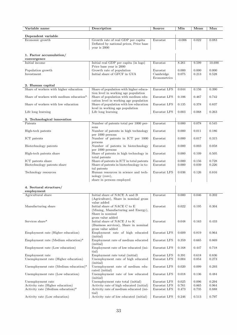
Variable name Description Source Min Mean Max

Dependent variableEconomic growth Growth rate of real GDP per capita Eurostat -0.006 0.022 0.083

Deflated by national prices, Price baseyear is 2000

1. Factor accumulation/convergenceInitial income Initial real GDP per capita (in logs) Eurostat 8.261 9.599 10.690

Price base year is 2000Population growth Growth rate of population Eurostat 0.000 0.000 0.000Investment Initial share of GFCF in GVA Cambridge 0.075 0.213 0.528

Econometrics

2. Human capitalShare of workers with higher education Share of population with higher educa-

tion level in working age populationEurostat LFS 0.044 0.156 0.390

Share of workers with medium education* Share of population with medium edu-cation level in working age population

Eurostat LFS 0.106 0.467 0.742

Share of workers with low education Share of population with low educationlevel in working age population

Eurostat LFS 0.135 0.378 0.837

Life long learning Life long learning Eurostat LFS 0.003 0.068 0.263

3. Technological innovationPatents Number of patents total per 1000 per-

sonsEurostat 0.000 0.078 0.545

High-tech patents Number of patents in high technologyper 1000 persons

Eurostat 0.000 0.011 0.186

ICT patents Number of patents in ICT per 1000persons

Eurostat 0.000 0.017 0.315

Biotechnology patents Number of patents in biotechnologyper 1000 persons

Eurostat 0.000 0.003 0.058

High-tech patents share Share of patents in high technology intotal patents

Eurostat 0.000 0.109 0.505

ICT patents share Share of patents in ICT in total patents Eurostat 0.000 0.156 0.728Biotechnology patents share Share of patents in biotechnology in to-

tal patentsEurostat 0.000 0.039 0.226

Technology resources Human resources in science and tech-nology (core),

Eurostat LFS 0.036 0.126 0.816

share in persons employed

4. Sectoral structure/employmentAgricultural share Initial share of NACE A and B Eurostat 0.000 0.046 0.202

(Agriculture), Share in nominal grossvalue added

Manufacturing share Initial share of NACE C to E Eurostat 0.022 0.195 0.304(Mining, Manufacturing and Energy),Share in nominalgross value added

Services share* Initial share of NACE J to K Eurostat 0.048 0.163 0.433(Business services), Share in nominalgross value added

Employment rate (Higher education) Employment rate of high educated(initial)

Eurostat LFS 0.609 0.819 0.964

Employment rate (Medium education)* Employment rate of medium educated(initial)

Eurostat LFS 0.359 0.665 0.869

Employment rate (Low education) Employment rate of low educated (ini-tial)

Eurostat LFS 0.168 0.447 0.718

Employment rate Employment rate total (initial) Eurostat LFS 0.391 0.618 0.836Unemployment rate (Higher education) Unemployment rate of high educated

(initial)Eurostat LFS 0.004 0.054 0.273

Unemployment rate (Medium education)* Unemployment rate of medium edu-cated (initial)

Eurostat LFS 0.020 0.099 0.293

Unemployment rate (Low education) Unemployment rate of low educated(initial)

Eurostat LFS 0.018 0.136 0.484

Unemployment rate Unemployment rate total (initial) Eurostat LFS 0.025 0.096 0.294Activity rate (Higher education) Activity rate of high educated (initial) Eurostat LFS 0.761 0.865 0.964Activity rate (Medium education)* Activity rate of medium educated (ini-

tial)Eurostat LFS 0.473 0.735 0.888

Activity rate (Low education) Activity rate of low educated (initial) Eurostat LFS 0.246 0.513 0.797

33

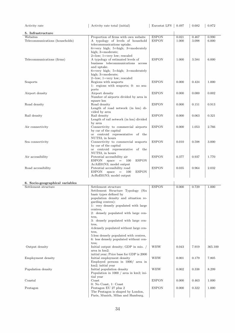
Activity rate Activity rate total (initial) Eurostat LFS 0.497 0.682 0.872

5. InfrastructureWebsites Proportion of firms with own website ESPON 0.021 0.467 0.990Telecommunications (households) A typology of levels of household

telecommunications uptake.ESPON 1.000 3.098 6.000

6=very high; 5=high; 3=moderatelyhigh; 3=moderate;2=low; 1=very low; rescaled

Telecommunications (firms) A typology of estimated levels of ESPON 1.000 3.584 6.000business telecommunications accessand uptake.6=very high; 5=high; 3=moderatelyhigh; 3=moderate;2=low; 1=very low; rescaled

Seaports Regions with seaports ESPON 0.000 0.424 1.0001: regions with seaports; 0: no sea-ports

Airport density Airport density ESPON 0.000 0.000 0.002Number of airports divided by area insquare km

Road density Road density ESPON 0.000 0.151 0.913Length of road network (in km) di-vided by area

Rail density Rail density ESPON 0.000 0.063 0.321Length of rail network (in km) dividedby area

Air connectivity Connectivity to commercial airportsby car of the capital

ESPON 0.000 1.053 2.766

or centroid representative of theNUTS3, in hours

Sea connectivity Connectivity to commercial seaportsby car of the capital

ESPON 0.010 0.598 3.000

or centroid representative of theNUTS3, in hours

Air accessibility Potential accessibility air ESPON 0.377 0.937 1.770ESPON space = 100 ESPONAcAiE01N3; model output

Road accessibility Potential accessibility road ESPON 0.035 0.964 2.032ESPON space = 100 ESPONAcRoE01N3; model output

6. Socio-geographical variablesSettlement structure Settlement structure ESPON 0.000 0.729 1.000

Settlement Structure Typology (Sixbasic types defined bypopulation density and situation re-garding centres):1: very densely populated with largecentres,2: densely populated with large cen-tres,3: densely populated with large cen-tres,4:densely populated without large cen-tres,5:less densely populated with centres,6: less densely populated without cen-tres;

Output density Initial output density; GDP in mio. /area in km2;

WIIW 0.043 7.919 365.100

initial year; Price base for GDP is 2000Employment density Initial employment density WIIW 0.001 0.179 7.805

Employed persons in 1000/ area inkm2; initial year

Population density Initial population density WIIW 0.002 0.338 8.299Population in 1000 / area in km2; ini-tial year

Coastal Coast ESPON 0.000 0.463 1.0000: No Coast, 1: Coast

Pentagon Pentagon EU 27 plus 2 ESPON 0.000 0.322 1.000The Pentagon is shaped by London,Paris, Munich, Milan and Hamburg.

34

Objective 1 Objective 1 regions ESPON 0.000 0.408 1.000Based on COM ’Second progress re-port on economicand social cohesion’ (30 January 2003)

Capital city Capital city 0.000 0.106 1.0000: region without capital cities; 1: cap-ital cities

Airports Number of airports ESPON 0.000 1.608 17.000Temperature Extreme temperatures, 2=Low

(Mean=2-2,75),ESPON 2.000 2.424 4.000

3=Moderate (Mean=2,75-3,25),4=High (Mean=3,25-3,50);calculated from NUTS3 digit; weightedby population shares

Hazard Sum of all weighted hazard values ESPON 100.000 232.000 307.300alculated from NUTS3; weighted bypopulation shares

Distance to Frankfurt Distance to Frankfurt in kmDistance to capital Distance to capital city in km 0.000 241.400 883.100

Table B.2: Data Description. Data are from ESPON (EuropeanSpatial Planning Observation Network), Cambridge Econometrics ,WIIW, Eurostat and Eurostat LFS (Eurostat Labor Force Survey).Variables expressed in shares additionally denoted by asterisks (*)are not included in the regressions and hence serve as a referencegroup.

35