The consumption-based determinants of theterm structure of discount rates1

Christian GollierUniversity of Toulouse and EIF

May 25, 2007

1An earlier version of this paper was entitled ”Transitory shocks to GNP andthe consumption-based term structure of interest rates”. I am indebted to JohnCampbell, Martin Weitzman and to two referees for helpful comments.

Abstract

The rate of return of a zero-coupon bond with maturity T is determinedby our expectations about the mean (+), variance (-) and skewness (+) ofthe growth of aggregate consumption between 0 and T . The shape of theyield curve is thus determined by how these moments vary with T . We firstexamine growth processes in which a higher past economic growth yields afirst-degree dominant shift in the distribution of the future economic growth,as assumed for example by Vasicek (1977). We show that when the growthprocess exhibits such a positive serial dependence, then the yield curve isdecreasing if the representative agent is prudent (u000 > 0), because of theincreased risk that it yields for the distant future. A similar definition isproposed for the concept of second-degree stochastic dependence, as observedfor example in the Cox-Ingersoll-Ross model, with the opposite comparativestatic property holding under temperance (u0000 < 0), because the change indownside risk (or skweness) that it generates. Finally, using these theoreticalresults, we propose two arguments in favor of using a smaller rate to discountcash-flows with very large maturities, as those associated to global warmingor nuclear waste management.Keywords: Stochastic dependence, yield curve, far distant future, pru-

dence, temperance, downside risk.JEL Classification: G12, E43, Q51

1 Introduction

How much effort are we ready to make today to improve the future? House-holds are faced with this question when they plan their savings for retirement,whereas entrepreneurs have to determine whether to undertake new invest-ment projects. At the collective level, one needs to determine, for example,whether to limit the national budget deficit, or whether to invest in the ed-ucation system. In a recent past, similar questions emerged, but with thestriking innovation of being related to the far-distant future. Exploring theuniverse, protecting the biodiversity, limiting the extraction of exhaustibleresources, dealing with nuclear wastes and global warming are a few exam-ples of policy questions that confront us to our attitude towards improvingthe welfare of human beings that will live in hundreds or thousands years inthe future. These valuation questions are all solved by the selection of thediscount rate.As is well-known, the use of a single rate to discount sure cash-flows at

all maturities implies that costs and benefits occurring, say, in more than100 years are typically irrelevant for the decision, because of the exponentialnature of discounting. This is why for example the so-called ”CopenhagenConsensus”1 ranked all projects linked to the prevention of global warmingat the lowest priority level based on standard cost-benefit analyses with aconstant discount rate. The problem is that there is a priori no scientific rea-son to believe that one should discount all maturities at the same rate. Thetradition of using a constant rate in cost-benefit analysis should not be seenas a dogma, but rather as a useful practical simplification. Various authors— among whom Weitzman (1998, 2001, 2004) is the most vocal — claimedthat one should opt for discount rates that are decreasing with the maturityof the cash flows under scrutiny. Weitzman (2004) in particular develops anargument for selecting a zero discount rate for maturities around 50 years,the discount rate becoming even negative for longer time horizons. Of course,adopting such recommendations would massively reallocate our collective in-vestments towards those benefiting to distant generations, potentially at thedetriment of actions with more immediate benefits such as fighting malariaand promoting education in developing countries. It is therefore important

1It is the outcome of a conference held in Copenhagen in May 2004 aimed at rankinga set of various collective investment projects, including fighting AIDS and malaria indeveloping countries, water management, biodiversity, education,....

1

to have a good understanding of the reasons why we should adopt such de-creasing discount rates.Since the seminal contribution of Vasicek (1977), economists have inten-

sively explored how efficient discount rates should vary with the maturity ofthe corresponding cash payment. The immense literature on the term struc-ture of interest rates has produced an important corpus of knowledge aboutthis question. It is quite unfortunate that researchers discussing this questionin the various forums of environmental economics do not take advantage ofthe existence of this vast literature.2 There are several reasons for that. First,most papers on the yield curve are aimed at explaining the observed shapeof that curve, whereas environmental economists have a much more norma-tive approach. Notice however that the absence of frictions in the standardmodels on the term structure implies that the equilibrium interest rates arealso the socially efficient discount rates to be used in cost-benefit analysis.Second, researchers in finance are usually interested in pricing traded assets,which implies that their time-horizon is limited by the largest maturity ofexisting liquid markets for risk-free assets, which does not exceed 30 years.Last but not least, this literature is highly complex, and it does usuallynot provide intuition to the underlying phenomena. This is well summarizedby Piazzesi (2005): ”The quest for understanding what moves bond yieldshas produced an enormous literature with its own journals and graduatecourses. Those who want to join the quest are faced with considerable obsta-cles. The literature has evolved mostly in continuous time, where stochasticcalculus reigns and partial differential equations spit fire. The knights inthis literature are fighting for different goals, which makes it often difficult tocomprehend why the quest is moving in certain directions.” This quest leadsto the (preliminary) conclusion that the shape of the yield curve is governedby the dynamics of the short term interest rate (and maybe a few otherstochastic factors) that may entails mean reversion together with temporaryand permanent shocks. Because the term structure is obtained by arbitrageusing an exogenously given dynamic process for the price kernel, this rea-soning is usually not based on individual preferences. It is therefore not aneasy starting block to explain to public decision-makers how much effort our

2See for example the collective book edited by Portney and Weyant (1999) on discount-ing. See also Arrow et al. (1996), Weitzman (1998, 2001), Newell and Pizer (2003) andGroom, Koundouri, Panopoulou and Pantelidis (2004).

2

generation should undertake to improve the welfare of future generations.The aim of this paper is twofold. First, we exhibit the fundamental

determinants of the shape of the yield curve based on the preferences of therepresentative agent and on the stochastic process of aggregate consumptionin the economy. Second, we examine realistic dynamic growth processes thatare relevant to determine the very long discount rates. We consider theclassical Lucas (1978)’s tree economy with an exogenous growth process toexamine these questions.The efficient interest rate associated to time horizon t is decreasing in

our willingness to save in order to finance consumption at that date, whichitself depends upon our expectations about the growth of our incomes over[0, t]. Therefore, the term structure of interest rates provides a rich set ofinformation about these expectations. For example, when consumers expectan increase in their future incomes, they want to cash this benefit imme-diately by reducing their saving. This raises the equilibrium interest rate.This wealth effect relies on the standard assumption that consumers wantto smooth their consumption over time. It explains why the yield curve isupward sloping when the representative agent expects an accelerating growthrate in the future (Estrella and Hardouvelis (1991)).Among the many difficulties to extract testable hypothesis about the

relationship between the term structure and expectations about the futureeconomic activity, the most important one is due to uncertainty. Since Leland(1968), we know that uncertainty about future incomes raises the prudentconsumers’ willingness to save. This precautionary effect tends to reduce theinterest rate. This implies for example that the anticipation of a deterministicreduction in the volatility of growth yields an increasing yield curve (Barsky(1989)). It is interesting to examine how does the accumulation of risk forlonger time horizons influence the determination of the corresponding interestrate. Because longer horizons mean larger expected consumption, peoplewant to save less for these better times. On the contrary, longer horizons alsomean more risk, which implies that consumers want to save more for thesemore uncertain times. Which of these wealth and precautionary effects willdominate the other? If the wealth effect dominates the precautionary effect,then the yield curve must be increasing.The simplest case is when the growth of the economy follows a station-

ary random process. In this case, both the expected log consumption andits variance increases proportionally with the time horizon. It implies that

3

the wealth effect and the precautionary effect exactly compensate each otherwhen the representative agent has a constant relative risk aversion (CRRA).As is well-known (see for example Mankiw (1981)), CRRA combined withan i.i.d. consumption growth process implies that the yield curve is com-pletely flat. In sections 3 and 4 of this paper, we show how the existence ofserial correlations in the growth rate of the economy affects the shape of theyield curve. We define two types of serial correlations. Positive first-degreestochastic dependence (FSD) occurs when an increase in the first subperiodgrowth rate induces a first-degree stochastic improvement in the conditionaldistribution of the growth rate in the second subperiod. Such a positive serialdependence in the growth of the economy tends to magnify the long-term riskon consumption relative to the short-term risk. It implies that the prudentrepresentative agent will want to rebalance her efforts towards the longertime horizons, thereby tending to reduce long interest rates. This is for-mally shown in section 3 in a much simpler and more intuitive way thantraditionally done in the existing literature. It is also more general in thesense that our result only requires that the representative agent be prudent.FSD dependence is the main feature of the two classical models of the termstructure, namely Vasicek (1977) and Cox, Ingersoll and Ross (1985a,b).There is positive second-degree stochastic dependence (SSD) in growth

rates if an increase in the first subperiod rate yields an increase in risk inthe conditional distribution of growth in the second subperiod. This tendsto raise the skewness of the distribution of future consumption. Ex ante, itreduces the expected marginal utility of wealth at that maturity if the fourthderivative of the utility function is negative, a condition that is satisfied forCRRA preferences. This tends to reduce the willingness to purchase morezero-coupon bonds associated to long maturities, thereby raising their rate ofreturn. This is proved in section 4. Notice that the main feature of the Cox-Ingersoll-Ross model is to add some SSD dependence in the Vasicek model.The link of our results to these two classical models are made more explicitin section 5.In section 6, we examine two specific stochastic processes with positive

FSD dependence that are realistic representations of the uncertainty facedby Humanity in the very long run. The first stochastic process for aggregateconsumption has a drift that can take two possible values. A switch fromone drift to the other can occur at each period with a very small probability.This is aimed at modeling the kind of event that we experienced with the

4

industrial revolution at the end of the 18th century, where the drift changedquite abruptly from the secular 0% per year to 2% per year since then.Our model formalizes the risk of a switch in the opposite direction — ”TheLimit to Growth” — due for example to the scarcity of natural resources orto the extinction of scientific progresses. We show that the positive FSDdependence that this stochastic process yields a strong negative effect on therate at which we should discount far-distant cash-flows. In the second modelof long-term uncertainty inspired from Weitzman (2004), we assume thatthe drift is unique but unknown. As time goes by, one will use Bayes rule toupdate the beliefs about the true value of the drift. This stochastic processalso yields positive FSD dependence — and thus decreasing discount rates —for the simple reason that a good news in the short term is a good news forthe secular distribution of growth.

2 The term structure

The preferences of the representative agent in the economy are representedby her utility function u and by her rate of pure preference for the present δ.The utility function u on consumption is assumed to be three times differ-entiable, increasing and concave. Let ect denote consumption at date t. Theequilibrium per period rate of return at date 0 for a zero-coupon bond matur-ing at date t is denoted rt. To be in equilibrium, investing marginally in suchan asset should leave the expected discounted utility of the representativeagent unchanged. This condition is written as

e−δtEu0 (ect) ertt = u0(c0), (1)

which is the standard Euler equation for the consumption-saving problem.On the right-hand side of this equality, u0(c0) is the welfare cost of reduc-ing consumption by one monetary unit, which is invested in the zero-couponbond. The left-hand side is the welfare benefit that such investment yields.Consumption at date t is increased by ertt, which yields an increase in ex-pected utility by Eu0 (ect) ertt, which must be discounted at rate δ to takeaccount of the delay. The classical consumption-based pricing formula is

5

obtained by rewriting condition (1) as

rt = δ − 1tln

Eu0(ect)u0(c0)

. (2)

Two factors determine by how much the risk-free rate exceeds the rate ofpure preference for the present δ. The first factor is a wealth effect. If weexpect to consume more in the future, i.e., if Eect > c0, the marginal utility ofone more euro in the future is smaller than the marginal utility of one moreeuro immediately: u0(Eect) < u0(c0). It implies that −t−1 ln(u0(Eect)/u0(c0))is positive. This positive wealth effect is increasing in the expected growthrate of consumption over the entire period [0, t] and in the rate at whichmarginal utility is decreasing with consumption, which is measured by theindex of relative risk aversion R(c) = −cu00(c)/u0(c). The intuition is thathigher expectations about future incomes reduces the willingness to save,thereby raising the equilibrium interest rate.But, except when marginal utility is linear, Eu0(ect) is not equal to u0(Eect),

which introduces a second factor to the determination of interest rates. Whenthe representative agent is prudent, i.e., when marginal utility is convex, theuncertainty surrounding future consumption raises the expected marginalutility: Eu0(ect) > u0(Eect). This raises the willingness to save, thereby yield-ing a reduction of the equilibrium interest rate. This precautionary effectgoes opposite to the wealth effect. It is increasing in the riskiness of futureconsumption and in the index of convexity of marginal utility, which is de-fined as relative prudence P (c) = −cu000(c)/u00(c). We can make thesedifferent factors more explicit by using second-order Taylor approximationsof u0(zt) in the above equality. This technique yields

rt ' δ +R(c0)Eect − c0

tc0− 12R(c0)P (c0)

V ar(ect/c0)t

, (3)

where the three terms in the right-hand side measure respectively the impa-tience effect, the wealth effect and the precautionary effect. This approxi-mation is exact for the instantaneous rate r0.The term structure of interest rate is determined by how these two con-

flicting factors are compounded over time. A more distant future usu-ally yields a larger expected consumption and a larger uncertainty. Therisk-averse and prudent representative agent’s willingness to purchase zero-

6

coupon bonds with that long maturity is reduced by the larger expected con-sumption, and is increased by the larger uncertainty. Therefore, as suggestedby approximation (3), an increasing (decreasing) yield curve is obtained if thewealth effect becomes more (less) dominant compared to the precautionaryeffect when considering longer time horizons.To illustrate, let us consider a simple case. Suppose that u(c) = c1−γ/(1−

γ), which implies that R(c) = γ and P (c) = γ + 1 for all c. Suppose alsothat the logarithm of consumption follows a stationary Brownian motion:3

d ln ct = µdt+ σdzt, (4)

where µ and σ are two scalars measuring respectively the mean and standarddeviation of the change in log consumption.

Proposition 1 Suppose that relative risk aversion is a constant γ and thatthe log of consumption follows a stationary Brownian motion with trend µand volatility σ. Then, the yield curve is flat with rt = r0 = δ+ γµ− 0.5γ2σ2for all t.

Proof: Because u0(c) = c−γ, we have that

Eu0(ect)u0(c0)

= E exp [−γ (lnect − ln c0)]By assumption, lnect−ln c0 is normally distributed with mean µt and varianceσ2t. We can thus rewrite the above equation as

Eu0(ect)u0(c0)

=1

σ√2πt

Zexp(−γz) exp

µ−(z − µt)2

2σ2t

¶dz.

This can be rewritten as

Eu0(ect)u0(c0)

= exp

µ−γµµt− γσ2t

2

¶¶ ∙1

σ√2πt

Zexp

µ−(z − (µt− γσ2t))2

2σ2t

¶dz

¸.

The bracketed term is the integral of the normal density function with meanµt− γσ2t and variance σ2t. This equals unity. Thus we obtain that

Eu0(ect)u0(c0)

= exp£−γ¡µt− 0.5γσ2t

¢¤.

3Using Ito’s Lemma, this is equivalent to assume that dc/c = (µ+ 0.5σ2)dt+ σdz.

7

Thus, using equation (2) yields4

rt = δ + γµ− 0.5γ2σ2. ¥ (5)

This formula is equivalent to those obtained by Mankiw (1981), Hansenand Singleton (1983), Breeden (1986) and Campbell (1986). It shows thatwhen relative risk aversion is constant(CRRA) and the growth rate of theeconomy follows a stationary Brownian motion, a longer time horizon yieldsan increase in the wealth effect and an increase in the precautionary effectthat exactly compensate each other, yielding a flat yield curve.Gollier (2002 a,b) characterized the conditions on preferences that im-

ply a monotone yield curve under the assumption of a stationary Brownianmotion. For example, he shows that increasing relative risk aversion impliesan increasing yield curve if the probability of recession is small enough. Inthis paper, we follow a more standard strategy which consists in relaxing theassumption of a stationary Brownian motion. This is relaxed by assumingthat the mean µ and/or the volatility σ of the consumption growth processare path-dependent, i.e., that the growth at time t depends upon the growthin the periods preceding t. In a word, we assume that future growth rates arepredictable. The typical methodology in the literature on the term structureof interest rates is to assume the following time series model:

d ln ct = µ(s)dt+ σc(s)dzt,

ds = g(s)dt+ σs(s)dzt.

Both the mean and the volatility of the growth rate of the economy areaffected by a state variable (also called a ”factor”) s that itself follows apotentially non-stationary Brownian motion. The special case of a deter-ministic process for the state variable (σs = 0) is easy to treat using theabove integration method. For example, when σc(s) ≡ σ, we easily obtain inthe CRRA case that

rt = δ + γm(t)− 0.5γ2σ2, (6)

4We can reconcile equations (3) and (5) by observing that the growth rate of expectedconsumption equals µ+ 0.5σ2. This implies that equation (5) can be rewritten as

rt = δ +RdEctct− 0.5RPσ2.

This proves that approximation (3) is exact in this case.

8

where m(t) = t−1R t0µ(s(τ))dτ is the mean change in log consumption in

period [0, t], and s(τ) is the solution of the differential equation s0 = g(s)with initial condition s(0) = s0. Only the wealth effect is affected by thedeterministic change in the expectation µ about the growth rate of the econ-omy. These changes in expectation explain why the yield curve is usuallynot flat for short and medium time-horizons. For example, the expectationof an accelerating growth implies an increasing yield curve. Observe from (6)that the unpredictable shocks in changes in log consumption have no effecton the shape of the yield curve. It only shifts it downwards.The complexity of the theory on the yield curve comes from the stochastic

component of the motion of the state variable s (σs 6= 0). In this paper, weisolate two effects of these predictable changes in expectations. Suppose firstthat the volatility σc of the growth rate of the economy is constant. Whenσc and σs have the same sign, and when µ is increasing in s, the expectedfuture growth rate of consumption is positively correlated with the short-term growth rate. More precisely, an increase in the stochastic componentdzt of the short-term growth yields a first-degree stochastic dominant shiftin the future growth rate. In section 3, we examine the effect of this positivecorrelation on the shape of the yield curve. Alternatively, suppose that theexpected growth rate µ of the economy is state-independent, and that thevolatility of the growth rate is increasing in the state variable. Then, ifσc and σs have the same sign, the volatility of the future growth rate ofthe economy is positively correlated with the short-term growth rate. Moreprecisely, an increase in the growth rate dzt in the short run yields a second-degree stochastic shift in the future growth rate. We examine the effect ofthis type of statistical relations on the shape of the yield curve in section 4.

3 First-degree stochastic dependence

In this section, we consider an arbitrary stochastic process for ect. We examinethe effect of positive serial dependence in changes in consumption on theinterest rate associated to maturity T. To do so, let us split period [0, T ]into two subperiods [0, t] and [t, T ]. Consider a random vector (ex1, ex2) whereex1 and ex2 denote the change in consumption respectively in period [0, t] and[t, T ]. It implies that consumption at date T equals c0+ex1+ex2. Let F denotethe distribution function of (ex1, ex2), and let F1 and F2 denote, respectively,

9

the marginal distributions of ex1 and ex2. Let also F2|1 be the conditionaldistribution of ex2 : F2|1(x1, x2) = Pr[ex2 < x2 | ex1 = x1]. We suppose thatthis distribution function exists.

Definition 1 Consider a pair of random variables (ex1, ex2). We say thatthere is positive FSD dependence between ex1 and ex2 if F2|1 is nonincreasingin x1 for all x2.

In other words, an increase in x1 generates a first-order stochastic dom-inant shift in the conditional distribution of ex2. In the statistical literature,this notion is referred to as the ”stochastic increasing positive dependence”,because ex2 is more likely to take on larger value when x1 increases (see forexample Joe (1997)). Milgrom (1981) uses this concept to define the notionof a good news. An example of stochastic process that satisfies the FSDproperty is the AR(1) process ex2 = φex1 + eε with a positive φ.The long-term interest rate in such an economy equals

rT = δ − 1

Tln

Eu0(c0 + ex1 + ex2)u0(c0)

. (7)

We want to compare this rate to the one that would prevail in an economywith the same marginal distributions for ex1 and ex2, but with no serial de-pendence between them. In the economy without any serial dependence, thelong-term interest rate would equal

riT = δ − 1

Tln

Eu0(c0 + ex1 + exi2)u0(c0)

, (8)

where (ex1, exi2) is a vector of independent random variables with distributionF1 and F2, respectively. Interest rate r

iT would be what one would obtain from

the calibrated model by assuming independence and by using the observedvariance of annual changes in consumption as the estimation of V ar(∆c).We want to determine the conditions under which rT is smaller than riT ,when ex2 exhibits positive FSD dependence with respect to ex1. There is asimple intuition for why this should be the case. The existence of a positivedependence in the changes in consumption tends to magnify the long-termrisk compared to short-term risks. This induces the prudent representativeagent to purchase more zero-coupon bonds with a long maturity, thereby

10

reducing the equilibrium long-term rate. Comparing (7) and (8) implies thatrT is smaller than riT if

Eu0(c0 + ex1 + ex2) ≥ Eu0(c0 + ex1 + exi2). (9)

The following Lemma is useful to examine this problem.

Lemma 1 Consider a differentiable bivariate function h . The following twoconditions are equivalent:

1. For any pair of random variables (ex1, ex2) that satisfies positive first-order dependence, we have that

Eh(ex1, ex2) ≥ Eh(ex1, exi2) (10)

2. h is supermodular, i.e., ∂h/∂x2 is increasing in x1.

Proof: See the appendix.5

Tchen (1980) showed a closely related result: If condition (10) is satisfiedfor all supermodular functions, then F (x1, x2) ≤ F1(x1)F2(x2) for all (x1, x2),i.e., (ex1, ex2) are ”positive quadrant dependent”, a concept weaker than FSDdependence.6 Shaked and Shanthikumar (2007) generalize these propertiesof ”supermodular orders” to more than two random variables.Applying this lemma to condition (9) requires using function h(x1, x2) =

u0(c0 + x1 + x2). It is supermodular if the representative agent is prudent.

Proposition 2 The presence of any positive first-order stochastic depen-dence in changes in consumption reduces the long-term risk-free rate if andonly if the representative agent is prudent.

This result confirms our intuition: positive FSD dependence in changes inconsumption raises the riskiness of consumption at date T, without changingits expected value. Under prudence, this reduces the interest rate associatedto maturity T . It tends to generate a downward-sloping yield curve.

5We can also prove that if h is supermodular, then condition (10) is satisfied if andonly if (ex1, ex2) exhibits positive FSC.

6See Joe (1997), Theorem 2.3.

11

It would have been more fashioned to define ex1 and ex2 as the (conditional)changes in log consumption over respectively subperiods [0, t] and [t, T ]. Thischange the nature of the comparative static exercise because the expectationof the log consumption is not the same as the log of the expectation ofconsumption. Because ecT = c0e

x1+x2 when xi denotes the change in logconsumption, we can use Lemma 1 to obtain the following alternative result.Observe that h(x1, x2) = u0(c0e

x1+x2) is supermodular if relative prudenceP (c) = −cu000(c)/u00(c) is larger than unity.

Proposition 3 The presence of any positive first-order stochastic depen-dence in changes in log consumption reduces the long-term risk-free rate ifand only if relative prudence is larger than unity.

Similarly, the long-term risk-free rate is increased by any negative FSDdependence if and only if relative prudence is larger than unity. Observe thatwhen relative risk aversion is constant (u(c) = c1−γ/(1−γ)), relative prudenceis also constant and is equal to relative risk aversion plus one. Thus, CRRAimplies that relative prudence is always larger than unity. When relative riskaversion is constant, positive (negative) FSD dependence in changes in logconsumption always reduces (raises) the long-term risk-free rate relative tothe benchmark of independent growth rates.

Corollary 1 Suppose that u is a power function and that changes in logconsumption (ex1, ex2) have the same marginals and exhibit positive first-orderstochastic dependence. It implies that the yield curve is decreasing: rT ≤ rt.

Proof: It is easy to check that the yield curve is flat (rit = riT ) in theeconomy with the independent growth rate (ex1, exi2). Because rt = rit andrT ≤ riT from Proposition 3, we obtain that rT ≤ rt in the economy with thepositively correlated growth rates (ex1, ex2). ¥Notice that positive FSD dependence alone is not sufficient to obtain a de-

creasing yield curve. The above corollary relied on the additional assumptionthat relative risk aversion is constant. More generally, going back to Propo-sition 3, relative prudence must be larger than unity to obtain that positiveFSD influences the long rate downwards. It is easy to exhibit utility func-tions that are concave but whose relative prudence is not larger than unity.For example, the simplest departure of CRRA with u(c) = (c+k)1−g/(1−g),

12

k > 0, implies a relative prudence P (c) = (1+g)c/(c+k). For such a concaveutility function, relative prudence tends to zero with c. At early stages ofits development, this economy may have an upward sloping yield curve evenif growth rates are positively FSD dependent. This comes from an implicitwealth increase. Observe that in spite of the fact that the dependence of(ex1, ex2) does not affect the expected cumulative change in log consumption, the expected cumulative change in the level of consumption is increasedby the presence of positive FSD dependence. This can be checked by usingfunction h(x1, x2) = ex1+x2 in the Lemma. This implicit increase in expectedfuture incomes reduces the willingness to save for the long term, and it re-quires an increase in the corresponding interest rate. Therefore, one needsa sufficiently strong precautionary effect to dominate this opposite wealtheffect. By Proposition 3, it requires that relative prudence be larger thanunity.

4 Second-degree stochastic dependence

A natural extension of this work is to examine economies where the changesin consumption ex1 and ex2 are statistically related according to the positivesecond-degree stochastic dependence (SSD) property. This is the case whenan increase in the first period change in consumption raises the risk associ-ated to the second period change in consumption in the sense of Rothschildand Stiglitz (1970). In other words, the volatility of economic growth is in-creased after a boom, and it is reduced after a downturn. An example ofsuch heteroskedastic process is ex2 = µ+ex1eε, with Eeε = 0 and eε independentof ex1.Definition 2 Consider a pair of random variables (ex1, ex2). We say thatthere is a positive SSD dependence between ex1 and ex2 if q(x2 | x1) = R x2 F2|1(x1, y)dyis non-decreasing in x1 for all x2, and if E [ex2 | x1] is independent of x1.We want to determine the effect of such statistical relationship in changes

in consumption over time on the long-term interest rate. As in the previoussection, we compare an economy (ex1, ex2) with positive SSD dependence withanother one (ex1, exi2) in which changes in consumption are serially indepen-dent with the same marginals. The following Lemma is helpful to solve thisproblem.

13

Lemma 2 Consider a twice differentiable bivariate function h . The follow-ing two conditions are equivalent:

1. For any pair of random variables (ex1, ex2) that satisfies positive second-order dependence, we have that

Eh(ex1, ex2) ≥ Eh(ex1, exi2) (11)

2. −∂h/∂x2 is supermodular, i.e., if ∂2h/∂x22 is non-increasing in x1.

Proof: See the appendix.Notice that if we apply this lemma to function h(x1, x2) = v(x1 + x2) for

any function v with a convex first derivative, we obtain the result that, underpositive SSD, ex1+ ex2 is a downside reduction in risk with respect to ex1+ exi2,as defined by Geiss, Menezes and Tressler (1980). It implies that these twosums have the same mean and the same variance, but the first has a largerskewness than the second. This is not a surprise since a downside reductionin risk is obtained by transferring zero-mean lotteries from low wealth statesto larger wealth levels, as explained by Eeckhoudt, Gollier and Schneider(1995).Applying this to the term structures given by (7) and (8) with h(x1, x2) =

u0(c0 + x1 + x2), we obtain the following Proposition.

Proposition 4 The presence of any positive second-degree stochastic depen-dence in changes in consumption raises the long-term risk-free rate if andonly if the third derivative of the utility function is non-increasing.

Observe that condition u0000 ≤ 0 — which is sometimes referred to as ”tem-perance” — is quite natural. It is necessary for the intuitive property thatabsolute prudence −u000/u00 is decreasing in wealth, as explained by Kimball(1990). Moreover, all CRRA functions satisfy this condition. There is asimple intuition for why a positive SSD in ∆c should raise the equilibriumlong-term rate. Indeed, a positive SSD implies an increase in skewness ofecT = c0+ex1+ex2. When u0000 is negative, the increased skewness in ecT reducesEu0(ecT ), which yields a reduction in the demand for the zero-coupon bondwhich matures at T. This raises its equilibrium rate of return. The assump-tion that the fourth derivative of the utility function is negative is compatible

14

with decreasing prudence (Kimball (1990)), and with risk vulnerability (Gol-lier and Pratt (1996)), two very intuitive behavioral assumptions.As in the previous section, we could have defined ex1 and ex2 as the

changes in log consumption. We should then use Lemma 2 with h(x1, x2) =u0(c0e

x1+x2). This yields the following result.

Proposition 5 Suppose that u is four times differentiable. The presence ofany positive second-order stochastic dependence in changes in log consump-tion raises the long-term risk-free rate if and only if f(c) = u00(c)+3cu000(c)+c2u0000(c) is uniformly negative.

When relative risk aversion is constant, f(c) equals −γ3c−γ−1 which isuniformly negative. This implies that a positive SSD dependence in ∆ ln calways raises the long-term interest rate for that family of utility functions.This tends to generate an upward-sloping yield curve. The proof of thefollowing corollary parallels the one of Corollary 1 and is therefore skipped.

Corollary 2 Suppose that u is a power function and that changes in logconsumption (ex1, ex2) have the same marginals and exhibit positive second-order stochastic dependence. It implies that the yield curve is increasing:rT ≥ rt.

Notice that condition f ≥ 0 in Proposition 5 adds the two terms u00 and3cu000 to condition u0000 < 0 in Proposition 4. The first additional term isdue to the fact that making changes in log consumption serially independentraises the expected consumption at T. This reinforces the initial reason fora longer long-term rate. Also, it yields an increase in the second moment ofecT . Under prudence, this tends to reduce the long-term rate. This explainsthe opposite term 3cu000 > 0 in the definition of function f . As said above,the two negative terms must always dominate this positive term in the caseof CRRA.

5 Relations with the existing literature on

the term structure

Our aim in this section is not to provide a survey of the enormous existingliterature on the term structure of interest rates. Rather, we want here to

15

illustrate our results by comparing them to those of the two most famoustime series models used in this literature: Vasicek (1977) and Cox, Ingersolland Ross (1985a,b). In most existing models of the term structure, the statevariable is the instantaneous interest rate r0. For example, in the modelof Vasicek (1977), the time series model for the stochastic discount factorΛ(t) = e−δtu0(ct)/u

0(c0) takes the following form:

dΛ

Λ= −r0dt− σΛdz

dr0 = φ(r − r0)dt+ σrdz.

The term structure is then obtained by rewriting the equilibrium condition(1) as rt = −t−1 lnEΛt. Parameter σr is the conditional volatility of theinstantaneous interest rate. Parameter φ controls mean reversion: if φ = 0,the instantaneous risk-free rate r0 exhibits no tendency to return to anyspecific value. When φ > 0, the instantaneous rate r0 is expected to returnto its mean r at rate φ. With a typical value of φ = 0.3 year−1, 7 this yieldsa half-life time of 2.3 years for a shock on the instantaneous interest rate.Assuming that u0(c) = c−γ, this model can be rewritten as8

d ln c =r0 − δ + 0.5σ2Λ

γdt+

σΛγdz (12)

dr0 = φ(r − r0)dt+ σrdz.

Campbell (1986) examines a more general (discrete) version of this modelin which the first difference of the log endowment follows a univariate, sta-tionary stochastic process with a constant drift. We recognize in equation(12) various elements affecting the yield curve. First, we observe that theconditional volatility of the growth rate of consumption is a constant σΛ/γ.This excludes the existence of SSD dependence. Second, when φ 6= 0, thereis a deterministic component in the expectations about the future growth of

7For example, Backus, Foresi and Telmer (1998) consider φ = 0.024 month−1.8By Ito’s Lemma, the reader can check that

−δdt− γd ln c = d lnΛ =dΛ

Λ− 0.5σ2Λdt.

16

the economy. When the current level of r0 is below r, one anticipates an ac-celerating economic growth, which makes the yield curve increasing for shortand medium maturities. In fact, when there is no serial dependence (σr = 0),using equation (6) yields

rt = r + (r0 − r)1− e−φt

φt(13)

The mean yield curve, which is obtained by taking r0 = r, is completelyflat in that case. Thus, a non-zero slope to the mean yield curve can beobtained only by introducing some permanency to shocks on ln c. Indeed,when σr 6= 0 and has the same sign as σΛ, there is positive FSD dependencein the time series of ∆ ln c. As claimed by Proposition 3, this tends toreduce the long-term interest rates, thereby yielding a reduction in the slopeof the yield curve. This is confirmed by the analytical solution obtainedby Vasicek (1977) which adds a third term υt in the right-hand side of(13), with υt being negative and decreasing in t when σrσΛ is positive.9 Inorder to explain the upward-sloping mean yield curve, as documented forexample by Backus, Foresi and Telmer (1998), one needs to have negativeFSD dependences in ∆ ln c. Assuming without loss of generality that σr ispositive, this requires that σΛ/γ be sufficiently negative. This sheds light onwhy ”a little experimentation tells us that σΛ governs the average slope ofthe yield curve, with negative values required to produce an upward slopewe observe in the data” (Backus, Foresi and Telmer (1998)).The Cox-Ingersol-Ross (CIR) model adds a square root terms in the

volatility, which makes it time-varying:

d ln c =r − δ + 0.5σ2Λ

γdt+

σΛ√r

γdz (14)

dr = φ(r − r)dt+ σr√rdz.

This implies that a positive shock on the state variable r increases both theshort term expected growth of the log consumption and its future volatility.

9Vasicek (1977) obtained

υt =

∙σ2r2φ2

+σrσΛφ

¸ ∙1− e−φt

φt− 1¸+

σ2r4φ3

¡1− e−φt

¢2t

.

17

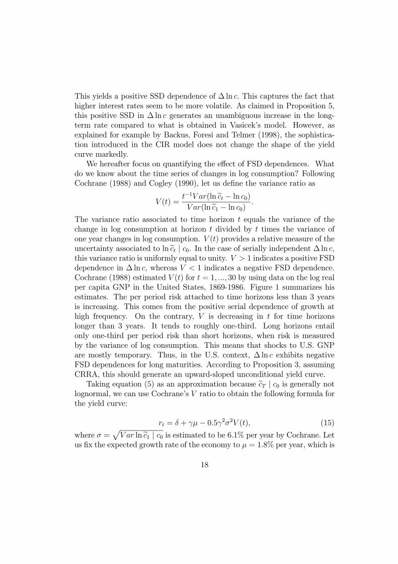
This yields a positive SSD dependence of ∆ ln c. This captures the fact thathigher interest rates seem to be more volatile. As claimed in Proposition 5,this positive SSD in ∆ ln c generates an unambiguous increase in the long-term rate compared to what is obtained in Vasicek’s model. However, asexplained for example by Backus, Foresi and Telmer (1998), the sophistica-tion introduced in the CIR model does not change the shape of the yieldcurve markedly.We hereafter focus on quantifying the effect of FSD dependences. What

do we know about the time series of changes in log consumption? FollowingCochrane (1988) and Cogley (1990), let us define the variance ratio as

V (t) =t−1V ar(lnect − ln c0)V ar(lnec1 − ln c0) .

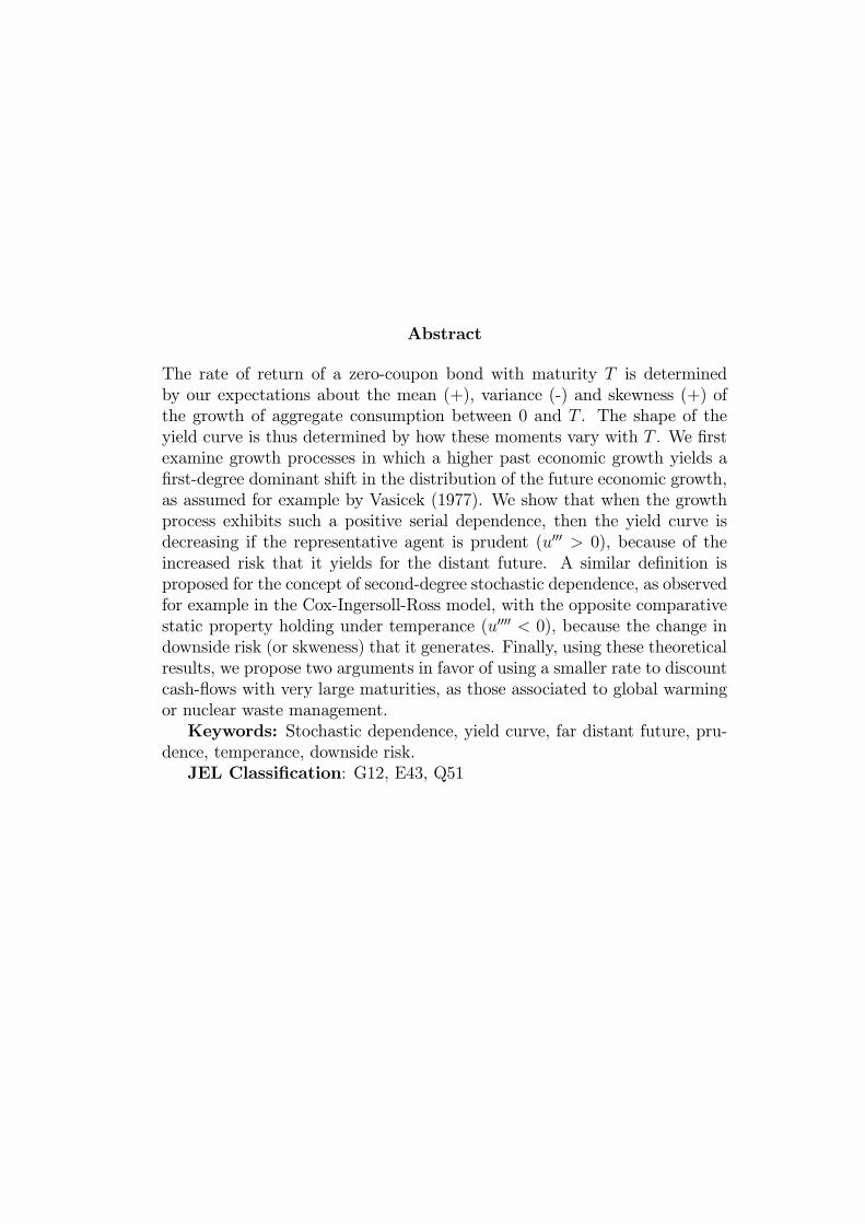
The variance ratio associated to time horizon t equals the variance of thechange in log consumption at horizon t divided by t times the variance ofone year changes in log consumption. V (t) provides a relative measure of theuncertainty associated to lnect | c0. In the case of serially independent ∆ ln c,this variance ratio is uniformly equal to unity. V > 1 indicates a positive FSDdependence in ∆ ln c, whereas V < 1 indicates a negative FSD dependence.Cochrane (1988) estimated V (t) for t = 1, ..., 30 by using data on the log realper capita GNP in the United States, 1869-1986. Figure 1 summarizes hisestimates. The per period risk attached to time horizons less than 3 yearsis increasing. This comes from the positive serial dependence of growth athigh frequency. On the contrary, V is decreasing in t for time horizonslonger than 3 years. It tends to roughly one-third. Long horizons entailonly one-third per period risk than short horizons, when risk is measuredby the variance of log consumption. This means that shocks to U.S. GNPare mostly temporary. Thus, in the U.S. context, ∆ ln c exhibits negativeFSD dependences for long maturities. According to Proposition 3, assumingCRRA, this should generate an upward-sloped unconditional yield curve.Taking equation (5) as an approximation because ecT | c0 is generally not

lognormal, we can use Cochrane’s V ratio to obtain the following formula forthe yield curve:

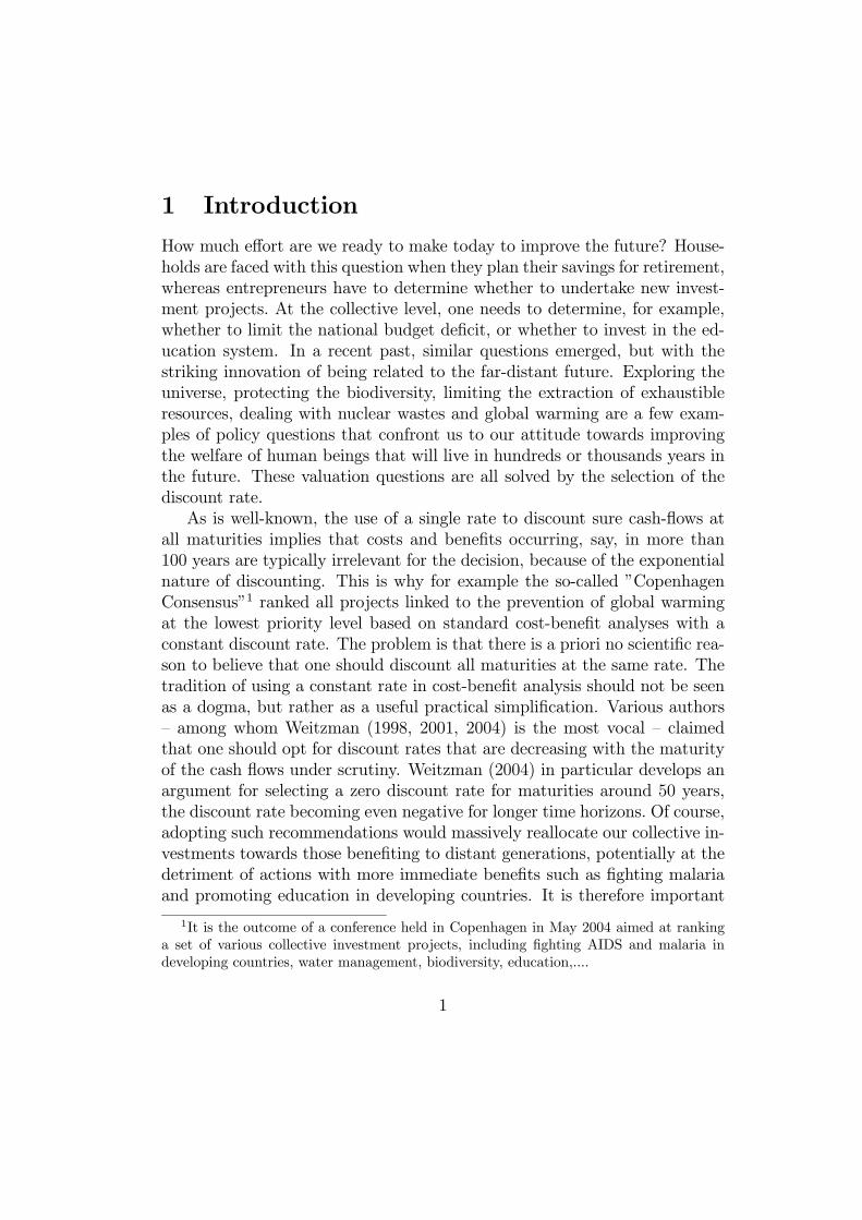
rt = δ + γµ− 0.5γ2σ2V (t), (15)

where σ =pV ar lnec1 | c0 is estimated to be 6.1% per year by Cochrane. Let

us fix the expected growth rate of the economy to µ = 1.8% per year, which is

18

0

0,2

0,4

0,6

0,8

1

1,2

1,4

0 5 10 15 20 25 30t

V(t)

Figure 1: The variance ratio for the log real per capita GNP, 1869-1986.(Source: Cochrane (1988)).

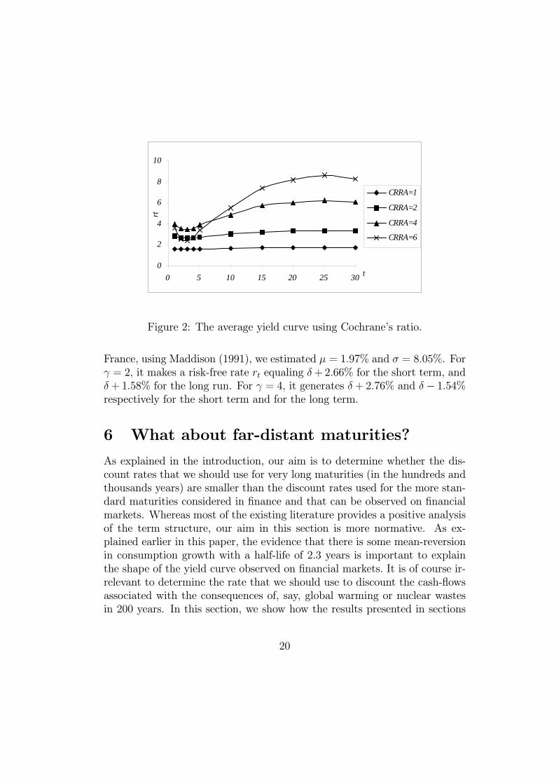
the average growth rate of real per capita consumption in the United Statesover the period 1889-1978 (Kocherlakota (1996)). In Figure 2, we draw theyield curve rt − δ computed from equation (15) for four different degrees ofrelative risk aversion: γ = 1, 2, 4 and 6. The upward-sloping shape of theaverage yield curve is familiar. Using U.S. monthly data from January 1952to February 1991, Backus, Foresi and Telmer (1998) estimated the mean 1-month yield to be 5.314%, going up to 6.693% for the yield corresponding toa 10-year maturity.Cogley (1990) showed that the pattern of the variance ratio exhibits much

differences across countries. In fact, the evidence indicates that the relativestability of long-term growth is unique to the United States. Using annualreal per capita GDP, 1871-1985, he computed the variance ratio V (20) fora twenty years horizon. He found 0.77 for Canada, which means that, asin the U.S. but at a smaller degree, this country should have a mean 20-year maturity yield that is larger than the short-term yield. He also found0.97 for Sweden, 1.03 for the United Kingdom, and 1.09 for Denmark. Theyield curve should be almost flat in these countries. But he also obtained1.4 for Australia, 1.84 for France and 2.02 for Italy. In these countries,the per-period growth risk is increasing with time horizon. It implies thatthe long-term interest rate should be smaller than the short-term one. For

19

0

2

4

6

8

10

0 5 10 15 20 25 30 t

rt

CRRA=1

CRRA=2

CRRA=4

CRRA=6

Figure 2: The average yield curve using Cochrane’s ratio.

France, using Maddison (1991), we estimated µ = 1.97% and σ = 8.05%. Forγ = 2, it makes a risk-free rate rt equaling δ+2.66% for the short term, andδ+ 1.58% for the long run. For γ = 4, it generates δ+ 2.76% and δ− 1.54%respectively for the short term and for the long term.

6 What about far-distant maturities?

As explained in the introduction, our aim is to determine whether the dis-count rates that we should use for very long maturities (in the hundreds andthousands years) are smaller than the discount rates used for the more stan-dard maturities considered in finance and that can be observed on financialmarkets. Whereas most of the existing literature provides a positive analysisof the term structure, our aim in this section is more normative. As ex-plained earlier in this paper, the evidence that there is some mean-reversionin consumption growth with a half-life of 2.3 years is important to explainthe shape of the yield curve observed on financial markets. It is of course ir-relevant to determine the rate that we should use to discount the cash-flowsassociated with the consequences of, say, global warming or nuclear wastesin 200 years. In this section, we show how the results presented in sections

20

3 and 4 are useful to make recommendations for such long time horizons.We examine two possible dynamic processes governing the long-term

growth of the economy. The first one involves Poisson jumps, whereas theother one exhibits some parameter uncertainty.

6.1 Two-state jumps in the growth of consumption

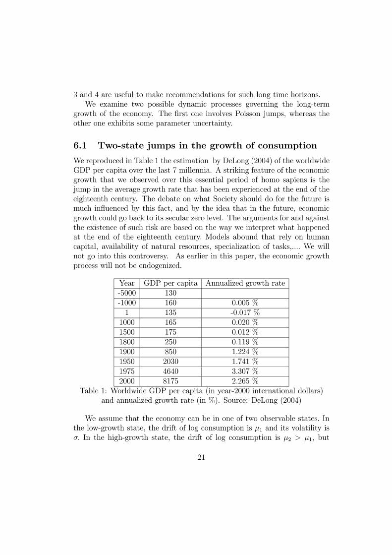
We reproduced in Table 1 the estimation by DeLong (2004) of the worldwideGDP per capita over the last 7 millennia. A striking feature of the economicgrowth that we observed over this essential period of homo sapiens is thejump in the average growth rate that has been experienced at the end of theeighteenth century. The debate on what Society should do for the future ismuch influenced by this fact, and by the idea that in the future, economicgrowth could go back to its secular zero level. The arguments for and againstthe existence of such risk are based on the way we interpret what happenedat the end of the eighteenth century. Models abound that rely on humancapital, availability of natural resources, specialization of tasks,.... We willnot go into this controversy. As earlier in this paper, the economic growthprocess will not be endogenized.

Year GDP per capita Annualized growth rate-5000 130-1000 160 0.005 %1 135 -0.017 %1000 165 0.020 %1500 175 0.012 %1800 250 0.119 %1900 850 1.224 %1950 2030 1.741 %1975 4640 3.307 %2000 8175 2.265 %

Table 1: Worldwide GDP per capita (in year-2000 international dollars)and annualized growth rate (in %). Source: DeLong (2004)

We assume that the economy can be in one of two observable states. Inthe low-growth state, the drift of log consumption is µ1 and its volatility isσ. In the high-growth state, the drift of log consumption is µ2 > µ1, but

21

the volatility remains the same. The economy switches from one state tothe other each time a Poisson event occurs. In discrete time, the model iswritten as

lnect+1 = ln ct + µt + σeεtµt+1 = (µt, 1− π;µ

0t, π),

where µ0t is µ2 if µt = µ1, otherwise µ0t = µ1. We assume that eεt is standard

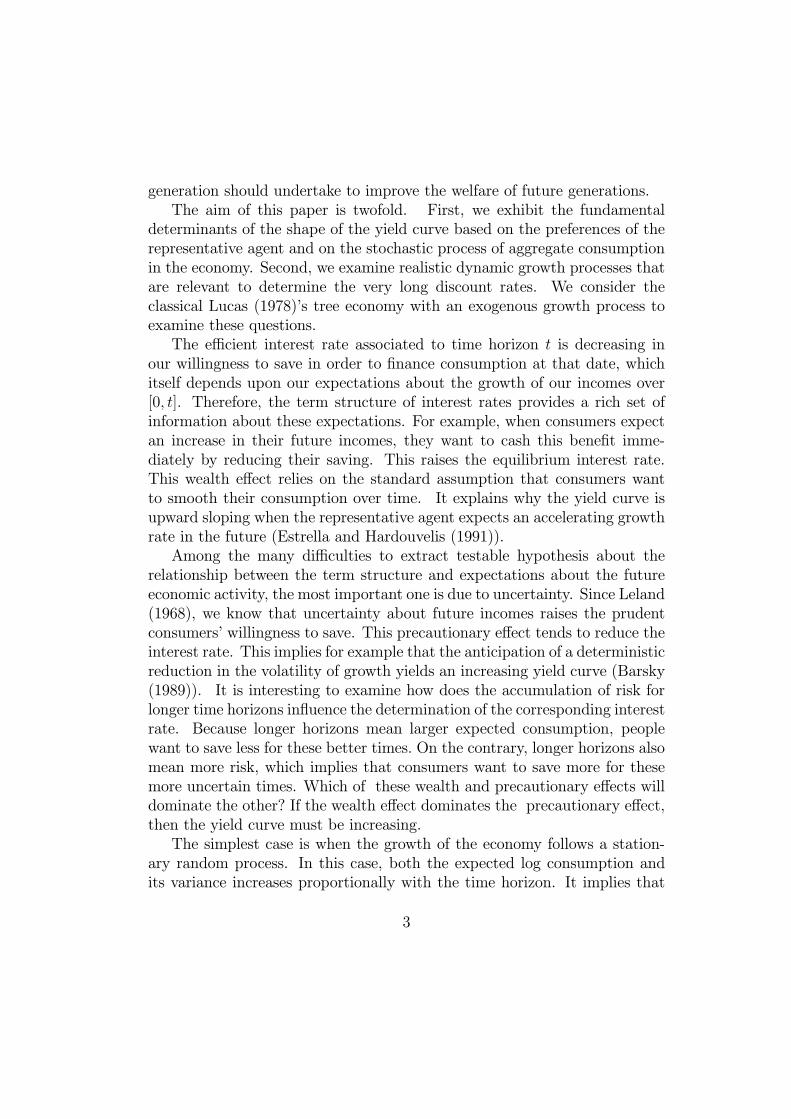
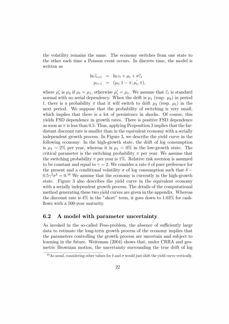
normal with no serial dependency. When the drift is µ1 (resp. µ2) in periodt, there is a probability π that it will switch to drift µ2 (resp. µ1) in thenext period. We suppose that the probability of switching is very small,which implies that there is a lot of persistence in shocks. Of course, thisyields FSD dependence in growth rates. There is positive FSD dependenceas soon as π is less than 0.5. Thus, applying Proposition 3 implies that the far-distant discount rate is smaller than in the equivalent economy with a seriallyindependent growth process. In Figure 3, we describe the yield curve in thefollowing economy: In the high-growth state, the drift of log consumptionis µ2 = 2% per year, whereas it is µ1 = 0% in the low-growth state. Thecritical parameter is the switching probability π per year. We assume thatthe switching probability π per year is 1%. Relative risk aversion is assumedto be constant and equal to γ = 2. We consider a rate δ of pure preference forthe present and a conditional volatility σ of log consumption such that δ −0.5γ2σ2 = 0.10 We assume that the economy is currently in the high-growthstate. Figure 3 also describes the yield curve in the equivalent economywith a serially independent growth process. The details of the computationalmethod generating these two yield curves are given in the appendix. Whereasthe discount rate is 4% in the ”short” term, it goes down to 1.03% for cash-flows with a 500-year maturity.

6.2 A model with parameter uncertainty

As invoked in the so-called Peso-problem, the absence of sufficiently largedata to estimate the long-term growth process of the economy implies thatthe parameters controlling the growth process are uncertain and subject tolearning in the future. Weitzman (2004) shows that, under CRRA and geo-metric Brownian motion, the uncertainty surrounding the true drift of log

10As usual, considering other values for δ and σ would just shift the yield curve vertically.

22

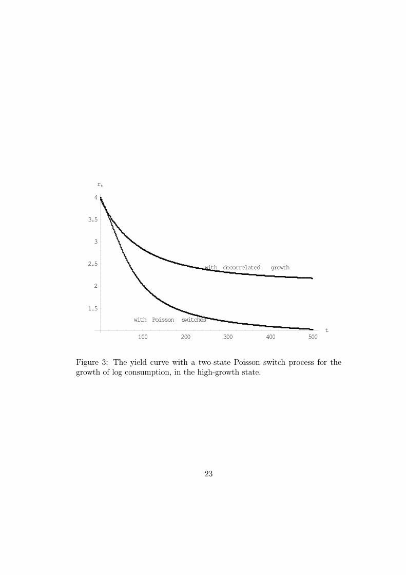
100 200 300 400 500t

1.5

2

2.5

3

3.5

4

rt

with decorrelated growth

with Poisson switches

Figure 3: The yield curve with a two-state Poisson switch process for thegrowth of log consumption, in the high-growth state.

23

consumption justifies selecting a smaller rate to discount distant cash-flows.In this section, we explain this phenomenon and we provide a more gen-eral model than in Weitzman (2004). The intuition for why the uncertaintysurrounding the drift of the growth process justifies selecting a smaller longdiscount rate is immediate from Proposition 2. Indeed, the observation ofa high growth in the short run induces the representative agent to reviseher expectations about the distribution of growth upwards. Thus, Bayesianlearning generates positive FSD dependence in the perceived growth process.This magnifies the long-term risk, thereby inducing the prudent representa-tive agent to make more effort for the distant future. As shown by Proposition2, this result requires no other restriction on preferences than prudence.We suppose that the growth process is stationary. Let ex(θ) denote the per-

period change in log consumption, conditional to parameter θ. The currentprior beliefs of the representative agent are described by the distribution ofrandom variable eθ. Under CRRA preferences, the current yield curve takesthe following form:11

rt = δ − 1tlnEα(eθ)t, (16)

where function α is defined as

α(θ) = Ee−γx(θ). (17)

Using Jensen’s inequality, we directly get the following result, which is relatedto Proposition 3.

Proposition 6 Suppose that the representative agent has CRRA preferences,and that the process of log consumption is stationary with an unknown pa-rameter θ. Under such circumstances, the socially efficient discount rate rtis non-increasing with time horizon t. It tends to the smallest possible rateminθ [δ − lnα(θ)] when t tends to infinity.

Proof: Observe first that function g(x) = x lnx is convex. Then, usingJensen’s inequality, we have that

t2Ehα(eθ)ti ∂rt

∂t=hEα(eθ)ti hlnEα(eθ)ti−E

hα(eθ)t lnα(eθ)ti

11In the economy with serial independence, we just have brt = δ − lnEα(eθ).24

is nonpositive. Thus, rt is non-increasing in t. Moreover, as is well-known,

when t tends to infinity,hEα(eθ)ti1/t tends to maxθ α(θ), which implies that

rt tends to δ − lnmaxθ α(θ).¥Notice that rt is strictly decreasing in t as soon as there exists two values

of the parameter, θ and θ0 such that α(θ) 6= α(θ0). This result and its proof isreminiscent — but is conceptually different — of a recommendation in Weitz-man (1998) for why ”the far-distant future should be discounted at its lowestpossible rate”. Notice also that the above result does not require any condi-tion on the distribution of changes in log consumption ex(θ), or on the priordistribution of parameter eθ. Weitzman (2004) assumes that ex(θ) is normalwith a known volatility σ, which implies that α(θ) = exp(−γµ(θ)+0.5γ2σ2).It implies in turn that the discount rate tends to δ− 0.5γ2σ2 + γminθ µ(θ).

Because he also assumes that µ(eθ) is normally distributed, the discount rategoes to minus infinity for large maturities under this specification!12

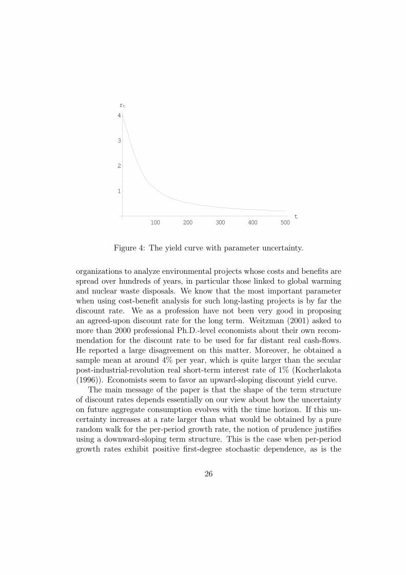
More realistic specifications of the per-period growth process and/or ofthe prior beliefs are thus welcomed. Equations (16) and (17) provide thissimple and flexible framework. Consider for example the following numericalillustration. The relative risk aversion of the representative agent equalsγ = 2. The change in log consumption is normal with conditional standarddeviation σ(θ)=6.1%, whereas we assume that δ − 0.5γ2σ2 = 0. The drift µis unknown, but it is either 3% or 0%. The prior belief is that there is a 2/3probability that the true drift is 3%, yielding an expected drift of 2%. If itwould be 3% for sure, the yield curve would be flat at 6%, whereas it wouldbe equal to 0% in the low-growth scenario. In Figure 4, we draw the yieldcurve given the current parameter uncertainty. The learning process inducesSociety to use today a 0.22% rate per year to discount cash-flows realized in500 years, whereas a discount rate of 4.0% per year is used for immediatebenefits and costs.

7 Conclusion

A correct assessment of how much Society should invest for its own future iscentral to economic analysis. Many of us are now cooperating with various

12If µ(eθ) is normally distributed with mean µ and variance σ20 , we obtain that rt =δ + γµ− 0.5γ2(σ2 + tσ20) which decreases linearly with the time horizon.

25

100 200 300 400 500t

1

2

3

4

rt

Figure 4: The yield curve with parameter uncertainty.

organizations to analyze environmental projects whose costs and benefits arespread over hundreds of years, in particular those linked to global warmingand nuclear waste disposals. We know that the most important parameterwhen using cost-benefit analysis for such long-lasting projects is by far thediscount rate. We as a profession have not been very good in proposingan agreed-upon discount rate for the long term. Weitzman (2001) asked tomore than 2000 professional Ph.D.-level economists about their own recom-mendation for the discount rate to be used for far distant real cash-flows.He reported a large disagreement on this matter. Moreover, he obtained asample mean at around 4% per year, which is quite larger than the secularpost-industrial-revolution real short-term interest rate of 1% (Kocherlakota(1996)). Economists seem to favor an upward-sloping discount yield curve.The main message of the paper is that the shape of the term structure

of discount rates depends essentially on our view about how the uncertaintyon future aggregate consumption evolves with the time horizon. If this un-certainty increases at a rate larger than what would be obtained by a purerandom walk for the per-period growth rate, the notion of prudence justifiesusing a downward-sloping term structure. This is the case when per-periodgrowth rates exhibit positive first-degree stochastic dependence, as is the

26

case with persistent shocks to growth rates, or when the drift of aggregateconsumption is unknown. Our calibrations induce us to recommend usingan average yearly discount rate of 4% for short-term cash-flows, and a yearlydiscount rate between 1% and 2% for time horizons exceeding 400 years.

27

REFERENCES

Arrow, K.J., W.R. Cline, K.-G. Maler, M. Munasinghe, R. Squitieriand J.E. Stiglitz, (1996), Intertemporal equity, discountingand economic efficiency, in Climate Change 1995 - Economicand Social Dimensions of Climate Change, eds J.P. Bruce, H.Lee and E.F. Haites, Cambridge University Press, CambridgeU.K..

Backus, D., S. Foresi and C. Telmer, (1998), Discrete-time modelsof bond pricing, NBER Working Paper 6736.

Barsky, R.B., (1989), Why don’t the prices of stocks and bondsmove together?, American Economic Review, 79, 1132-1145.

Campbell, (1986), Bond and stock returns in a simple exchangemodel, Quarterly Journal of Economics, 101, 785-804.

Cochrane, J.H., (1988), How big is the random walk in GNP?,Journal of Political Economy, 96, 893-920.

Cochrane, J., (2001), Asset Pricing, Princeton University Press.

Cogley, T., (1990), International evidence on the size of the ran-dom walk in output, Journal of Political Economy, 98, 501-518.

Cox, J., Ingersoll, J., and S. Ross, (1985a), A theory of the termstructure of interest rates, Econometrica, 53, 385-403.

Cox, J., Ingersoll, J., and S. Ross, (1985b), An intertemporalgeneral equilibrium model of asset prices, Econometrica, 53,363-384.

Breeden, D.T., (1986), Consumption, production, inflation, andinterest rates: A synthesis, Journal of Financial Economics,16, 3-40.

DeLong, B.J., (2004), Chapter 5: The reality of economic growth:History and prospect, http://www.j-bradford-delong.net.

Eeckhoudt, L., C. Gollier. and T. Schneider, (1995), Risk aver-sion, prudence and temperance: A unified approach, Eco-nomics Letters, 48, 331-336.

28

Estrella, A., and G.A. Hardouvelis, (1991), The term structureas a predictor of real economic activity, Journal of Finance,46, 555-576.

Geiss, C. , C. Menezes and J. Tressler, (1980), Increasing Down-side Risk, American Economic Review, 70, 5, 921-931.

Gollier, C., (2002a), Discounting an uncertain future, Journal ofPublic Economics, 85, 149-166.

Gollier, C., (2002b), Time horizon and the discount rate, Journalof Economic Theory, 107, 463-473.

Gollier, C. and J.W. Pratt, (1996), Risk vulnerability and thetempering effect of background risk, Econometrica, 64, 1109-1124.

Groom, B., Koundouri, P., Panipoulou, K., and T., Pantelides,(2007), Discounting the Distant Future: Howmuch does modelselection affect the certainty equivalent rate? Journal of Ap-plied Econometrics. 22:641-656.

Hansen, L. and K. Singleton, (1983), Stochastic consumption,risk aversion and the temporal behavior of assets returns,Journal of Political Economy, 91, 249-265.

Joe, H., (1997), Multivariate models and dependence concepts,Chapman and Hall/CRC.

Kimball, M.S., (1990), Precautionary savings in the small and inthe large, Econometrica, 58, 53-73.

Kocherlakota, N.R., (1996), The Equity Premium: It’s Still aPuzzle, Journal of Economic Literature, 34, 42-71.

Lehmann, E.L., (1966), Some concepts of dependence, Annals ofMathematical Statistics, 37, 1137-1153.

Leland, H., (1968), Savings and uncertainty: The precautionarydemand for savings, Quarterly Journal of Economics, 45, 621-36.

Lucas, R., (1978), Asset prices in an exchange economy, Econo-metrica, 46, 1429-46.

29

Maddison, A., (1991), Phases of Economic Development, OxfordEconomic Press.

Mankiw, G., (1981), The permanent income hypothesis and thereal interest rate, Economic Letters, 7, 307-311.

Milgrom, P., (1981), Good news and bad news: Representationtheorems and applications, Bell Journal of Economics, 12,380-91.

Newell, R., and W. Pizer, (2003), Discounting the benefits of cli-mate change mitigation: How much uncertain rates increasevaluations?, Journal of Environmental Economics and Man-agement, 46 (1), 52-71.

Piazzesi, M., (2005), Affine term structure models, in Handbookof Financial Econometrics, Y. Ait-Sahalia and L.P. Hanseneds, Elsevier.

Portney, P.R., and J. P. Weynant, eds., (1999), Discounting andintergenerational equity, Resources for the future, Washing-ton, D.C..

Rothschild, M. and J. Stiglitz, (1970), Increasing risk: I. A defi-nition, Journal of Economic Theory, 2, 225-243.

Shaked, M., and J.G. Shanthikumar, (2007), Stochastic Orders,Springer series in statistics.

Tchen, A.H., (1980), Inequalities for distributions with givenmarginals, Annals of Probability, 8, 814-827.

Vasicek, 0., (1977), An equilibrium characterization of the termstructure, Journal of Financial Economics, 5, 177-188.

Weitzman, M.L., (1998), Why the far-distant future should bediscounted at its lowest possible rate?, Journal of Environ-mental Economics and Management, 36, 201-208.

Weitzman, M.L., (2001), Gamma discounting, American Eco-nomic Review, 91, 260-271.

Weitzman, M.L., (2004), Statistical discounting of an uncertaindistant future, mimeo, Harvard University.

30

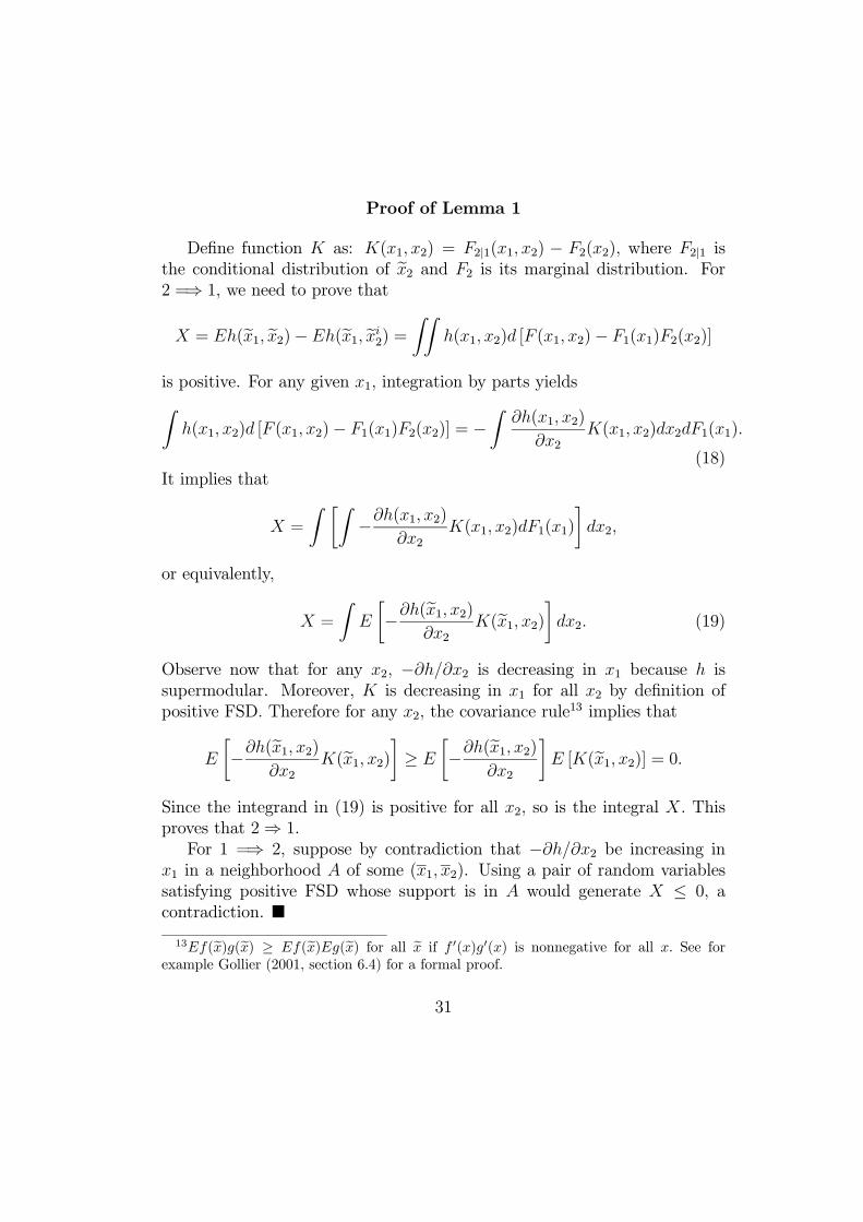
Proof of Lemma 1

Define function K as: K(x1, x2) = F2|1(x1, x2) − F2(x2), where F2|1 isthe conditional distribution of ex2 and F2 is its marginal distribution. For2 =⇒ 1, we need to prove that

X = Eh(ex1, ex2)−Eh(ex1, exi2) = ZZ h(x1, x2)d [F (x1, x2)− F1(x1)F2(x2)]

is positive. For any given x1, integration by parts yieldsZh(x1, x2)d [F (x1, x2)− F1(x1)F2(x2)] = −

Z∂h(x1, x2)

∂x2K(x1, x2)dx2dF1(x1).

(18)It implies that

X =

Z ∙Z−∂h(x1, x2)

∂x2K(x1, x2)dF1(x1)

¸dx2,

or equivalently,

X =

ZE

∙−∂h(ex1, x2)

∂x2K(ex1, x2)¸ dx2. (19)

Observe now that for any x2, −∂h/∂x2 is decreasing in x1 because h issupermodular. Moreover, K is decreasing in x1 for all x2 by definition ofpositive FSD. Therefore for any x2, the covariance rule

13 implies that

E

∙−∂h(ex1, x2)

∂x2K(ex1, x2)¸ ≥ E

∙−∂h(ex1, x2)

∂x2

¸E [K(ex1, x2)] = 0.

Since the integrand in (19) is positive for all x2, so is the integral X. Thisproves that 2⇒ 1.For 1 =⇒ 2, suppose by contradiction that −∂h/∂x2 be increasing in

x1 in a neighborhood A of some (x1, x2). Using a pair of random variablessatisfying positive FSD whose support is in A would generate X ≤ 0, acontradiction. ¥13Ef(ex)g(ex) ≥ Ef(ex)Eg(ex) for all ex if f 0(x)g0(x) is nonnegative for all x. See for

example Gollier (2001, section 6.4) for a formal proof.

31

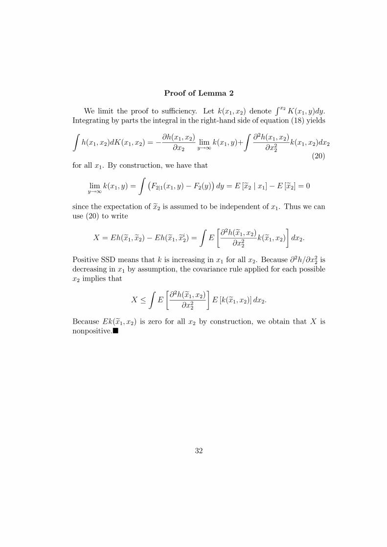
Proof of Lemma 2

We limit the proof to sufficiency. Let k(x1, x2) denoteR x2 K(x1, y)dy.

Integrating by parts the integral in the right-hand side of equation (18) yieldsZh(x1, x2)dK(x1, x2) = −

∂h(x1, x2)

∂x2limy→∞

k(x1, y)+

Z∂2h(x1, x2)

∂x22k(x1, x2)dx2

(20)for all x1. By construction, we have that

limy→∞

k(x1, y) =

Z ¡F2|1(x1, y)− F2(y)

¢dy = E [ex2 | x1]−E [ex2] = 0

since the expectation of ex2 is assumed to be independent of x1. Thus we canuse (20) to write

X = Eh(ex1, ex2)−Eh(ex1, exi2) = Z E

∙∂2h(ex1, x2)

∂x22k(ex1, x2)¸ dx2.

Positive SSD means that k is increasing in x1 for all x2. Because ∂2h/∂x22 is

decreasing in x1 by assumption, the covariance rule applied for each possiblex2 implies that

X ≤Z

E

∙∂2h(ex1, x2)

∂x22

¸E [k(ex1, x2)] dx2.

Because Ek(ex1, x2) is zero for all x2 by construction, we obtain that X isnonpositive.¥

32

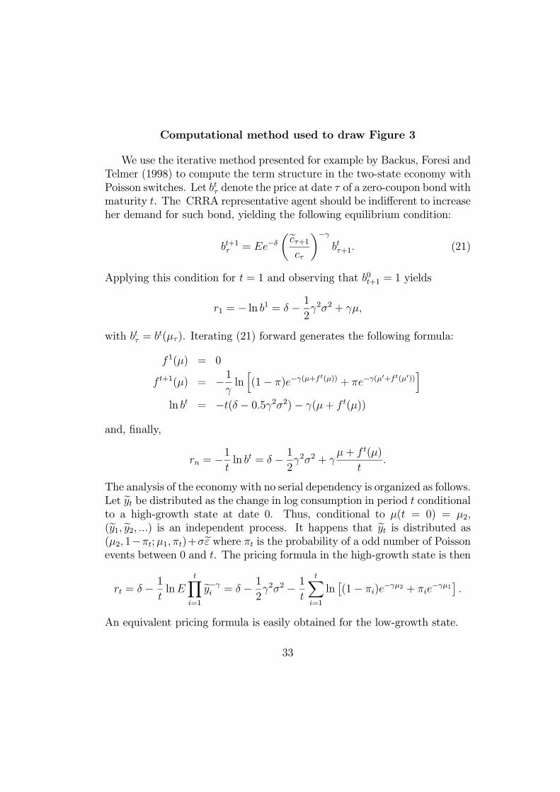
Computational method used to draw Figure 3

We use the iterative method presented for example by Backus, Foresi andTelmer (1998) to compute the term structure in the two-state economy withPoisson switches. Let btτ denote the price at date τ of a zero-coupon bond withmaturity t. The CRRA representative agent should be indifferent to increaseher demand for such bond, yielding the following equilibrium condition:

bt+1τ = Ee−δµecτ+1

cτ

¶−γbtτ+1. (21)

Applying this condition for t = 1 and observing that b0t+1 = 1 yields

r1 = − ln b1 = δ − 12γ2σ2 + γµ,

with btτ = bt(µτ ). Iterating (21) forward generates the following formula:

f1(µ) = 0

f t+1(µ) = −1γlnh(1− π)e−γ(µ+f

t(µ)) + πe−γ(µ0+ft(µ0))

iln bt = −t(δ − 0.5γ2σ2)− γ(µ+ f t(µ))

and, finally,

rn = −1

tln bt = δ − 1

2γ2σ2 + γ

µ+ f t(µ)

t.

The analysis of the economy with no serial dependency is organized as follows.Let eyt be distributed as the change in log consumption in period t conditionalto a high-growth state at date 0. Thus, conditional to µ(t = 0) = µ2,(ey1, ey2, ...) is an independent process. It happens that eyt is distributed as(µ2, 1−πt;µ1, πt)+σeε where πt is the probability of a odd number of Poissonevents between 0 and t. The pricing formula in the high-growth state is then

rt = δ − 1tlnE

tYi=1

ey−γi = δ − 12γ2σ2 − 1

t

tXi=1

ln£(1− πi)e

−γµ2 + πie−γµ1

¤.

An equivalent pricing formula is easily obtained for the low-growth state.

33