the consumer - Εθνικό και Καποδιστριακό ... · chapter 4 the consumer...

Chapter 4

The Consumer

Consumer : A person who is capable of choosing a president but inca-pable of choosing a bicycle without help from a government agency.ñ Herbert Stein, Washington Bedtime Stories (1979)

4.1 Introduction

It is now time to introduce the second of the principal economic actors in the eco-nomic system ñ the consumer. In a sense this is the heart of the microeconomics.Why else speak about ìconsumer sovereigntyî? For what else, ultimately, is theeconomyís productive activity organised?We will tackle the economic principles that apply to the analysis of the

consumer in the following broad areas:

! Analysis of preferences.

! Consumer optimisation in perfect markets.

! Consumerís welfare.

This, of course, is just an introduction to the economics of individual con-sumers and households; in this chapter we concentrate on just the consumer inisolation. Issues such as the way consumers behave en masse in the market, theissues concerning the supply by households of factors such as labour and savingsto the market and whether consumers ìsubstituteî for the market by produc-ing at home are deferred until chapter 5. The big topic of consumer behaviourunder uncertainty forms a large part of chapter 8.In developing the analysis we will see several points of analogy where we can

compare the theory of consumer with the theory of the Örm. This can make lifemuch easier analytically and can give us several useful insights into economicproblems in both Öelds of study.

69

70 CHAPTER 4. THE CONSUMER

Figure 4.1: The consumption set: standard assumptions

4.2 The consumerís environment

As with the Örm we begin by setting out the basic ingredients of the problem.First, a preliminary a word about who is doing the consuming. I shall sometimesrefer to ìthe individual,î sometimes to ìthe householdî and sometimes ñ morevaguely ñ to ìthe consumer,î as appropriate. The distinction does not matteras long as (a) if the consumer is a multiperson household, that householdísmembership is taken as given and (b) any multiperson household acts as thoughit were a single unit. However, in later work the distinction will indeed matterñ see chapter 9.Having set aside the issue of the consumer we need to characterise and discuss

three ingredients of the basic optimisation problem:

! the commodity space;

! the market;

! motivation.

The commodity space.

We assume that there is a known list of n commodities where n is a Önite,but perhaps huge, number. A consumption is just a list of commodities x :=

4.2. THE CONSUMERíS ENVIRONMENT 71

Figure 4.2: Two versions of the budget constraint

(x1; x2; :::; xn). We shall refer to the set of all feasible consumption bundles asX. In most cases we shall assume that X is identical to Rn+, the set of all non-negative n-vectors ñ see Figure 4.1; the implications of this are that a negativeamount of any commodity makes no sense, that all commodities are divisible,and there is no physical upper bound to the amount of any one commodity thatan individual could consume (that bound is going to be set by the budget, whichwe will come to in a moment).1

How do you draw the boundaries of goods classiÖcations? This depends onthe type of model you want to analyse. Very often you can get by with caseswhere you only have two or three commodities ñ and this is discussed furtherin chapter 5. Commodities could, in principle, be di§erentiated by space, time,or the state-of-the-world.

The market.

As in the case of the competitive Örm, we assume that the consumer has accessto a market in which the prices of all n goods are known: p := (p1; p2; :::; pn).These prices will, in part, determine the individualís budget constraint.However, to complete the description, there are two versions (at least) of this

constraint which we may wish to consider using in our model of the consumer.

1 How might one model indivisibilities in consumption? Describe the shape of the set Xif good 1 is food, and good 2 is (indivisible) refrigerators.


These two versions are presented in Figure 4.2.

! In the left-hand version a Öxed amount of money y is available to theconsumer, who therefore Önds himself constrained to purchase a bundle ofgoods x such that

p1x1 + p2x2 " y: (4.1)

if all income y were spent on good 1 the person would be able to buy aquantity x1 = y=p1.

! In the right-hand version the person has an endowment of resources R :=(R1; R2), and so his chosen bundle of goods must satisfy

p1x1 + p2x2 " p1R+ p2R2: (4.2)

The two versions of the budget constraint look similar, but will induce dif-ferent responses when prices change.2

Motivation.

This is not so easy to specify as in the case of the Örm, because there is no over-whelmingly strong case for asserting that individuals or households maximisea particular type of objective function if, indeed anything at all. Householdscould conceivably behave in a frivolous fashion in the market (if Örms behavein a frivolous fashion in the market then presumably they will go bust). Butif they are maximising something, what is it that they are maximising? Wewill examine two approaches that have been attempted to this question, each ofwhich has important economic applications. In the Örst we suppose that peoplemake their choices in a way that reveals their own preferences. Secondly weconsider a method of introspection.

4.3 Revealed preference

We shall tackle Örst the di¢cult problem of the consumerís motivation. To someextent it is possible to deduce a lot about a Örmís objectives, technology andother constraints from external observation of how it acts. For example fromdata on prices and on Örmsí costs and revenue we could investigate whetherÖrmsí input and output decisions appear to be consistent with proÖt maximi-sation. Can the same sort of thing be done with regard to consumers?The general approach presupposes that individualsí or householdsí actions in

the market reáect the objectives that they were actually pursuing, which mightbe summarised as ìwhat-you-see-is-what-they-wantedî.

2 (i) For each type of budget constraint sketch what will happen if the price of good 1 falls.(ii) Repeat this exercise for a rise in the price of good 2. (iii) Redraw the right-hand casefor the situation in which the price at which one can buy a commodity is greater than theprice at which one can sell the same commodity.

4.3. REVEALED PREFERENCE 73

xi amount consumed of good ix (x1; :::; xn)X the set of all xpi price of good ip (p1; :::; pn)y income

< weak preference relationB revealed preference relationU utility function) utility level

Table 4.1: The Consumer: Basic Notation

DeÖnition 4.1 A bundle x is revealed preferred to a bundle x0 (written insymbols x B x0) if x is actually selected when x0 was also available to the con-sumer.

The idea is almost self-explanatory and is given operational content by thefollowing axiom.

Axiom 4.1 (Axiom of rational choice) The consumer always makes a choice,and selects the most preferred bundle that is available.

This means that we can draw inferences about a personís preferences byobserving the personís choices; it suggests that we might adopt the followingsimple ñ but very powerful ñ assumption.

Axiom 4.2 (Weak Axiom of Revealed Preference) If x B x0 then x0 7x:

In the case where purchases are made in a free market this has a very simpleinterpretation. Suppose that at prices p the household could a§ord to buyeither of two commodity bundles, x or x0; assume that x is actually bought.Now imagine that prices change from p to p0 (while income remains unchanged);if the household now selects x0 then the weak axiom of revealed preference statesthat x cannot be a§ordable at the new prices p0. Thus the axiom means thatif

nX

i=1

pixi !nX

i=1

pix0i (4.3)

thennX

i=1

p0ixi >

nX

i=1

p0ix0i (4.4)

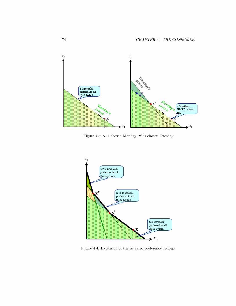
If you do not choose today something that you chose yesterday (when todayísbundle was also available and a§ordable) it must be because now you cannota§ord yesterdayís bundle: see Figure 4.3.


Figure 4.3: x is chosen Monday; x0 is chosen Tuesday

Figure 4.4: Extension of the revealed preference concept

4.4. PREFERENCES: AXIOMATIC APPROACH 75

You can get a long way in consumption theory with just this. Indeed with alittle experimentation it seems as though we are almost sketching out the resultof the kind of cost-minimisation experiment that we performed for the Örm, inwhich we traced out a portion of a contour of the production function. Perhapswe might even suspect that we are on the threshold of discovering a counterpartto isoquants by the back door (we come to a discussion of ìindi§erence curvesîon page 77 below). For example, examine Figure 4.4: let x B x0, and x0B x00,and let N(x) denote the set of points to which x is not revealed-preferred. Nowconsider the set of consumptions represented by the unshaded area: this is N(x)\ N(x0)\N(x00) and since x is revealed preferred to x0 (which in turn is revealedpreferred to x00 we might think of this unshaded area as the set of points whichare ñ directly or indirectly ñ revealed to be at least as good as x00: the set isconvex and the boundary does look a bit like the kind of contour we discussed inproduction theory. However, there are quite narrow limits to the extent that wecan push the analysis. For example, it would be possible to have the followingkind of behaviour: x B x0, x0 B x00, x00B x000 and yet also x000 B x. To avoid thisproblem actually you need an additional axiom ñ the Strong Axiom of RevealedPreference which explicitly rules out cyclical preferences.

4.4 Preferences: axiomatic approach

In contrast to section 4.3 let us use the method of introspection. Instead ofjust drawing inferences from peopleís purchases, we approach the problem ofspecifying their preferences directly. We proceed by setting out a number ofaxioms which it might be reasonable to suppose that a consumerís preferencesshould satisfy. There is no special magic in any one axiom or set of axioms:they are just a way of trying to capture a structure that seems appropriate inthe light of everyday experience. There is a variety of ways in which we mightcoherently axiomatise a model of consumer choice. Our fundamental conceptis:

DeÖnition 4.2 The weak preference relation < is a binary relation on X. Ifx;x0 2 X then the statement ìx < x0î is to be read ìx is at least as good as x0î.

To make this concept useful we shall consider three basic axioms on prefer-ence.

Axiom 4.3 (Completeness) For every x;x0 2 X, either x < x0 is true, orx0 < x is true, or both statements are true.

Axiom 4.4 (Transitivity) For any x;x0;x00 2 X, if both x < x0 and x0 < x00,then x < x00.


Axiom 4.5 (Continuity) 3 For any x 2 X, the not-better-than-x set and thenot-worse-than-x set are closed in X.

Figure 4.5: The continuity axiom

Completeness means that people do not shrug their shoulders helplessly whenconfronted with a choice; transitivity implies that (in a sense) they are consis-tent.4 To see what the continuity axiom implies do the experiment illustratedin Figure 4.5. In a two-commodity diagram put some point x! that representspositive amounts of both goods; plot any other point xM that represents more ofboth goods, and some other point xL that represents less of both goods (relativeto x!); suppose the individual strictly prefers xM to x! and x! to xL. Now con-sider points in the line

!xL;xM

": clearly points ìcloseî to xM may reasonably

3 What are the implications of dropping the continuity assumption?4 Each day I buy one piece of fruit for my lunch. On Monday apples and bananas are

available, but no oranges: I buy an apple. On Tuesday bananas and oranges are available,but no apples: I buy a banana. On Wednesday apples and oranges are available (sorry wehave no bananas): I buy an orange. Am I consistent?


Figure 4.6: Two utility functions representing the same preferences

be considered to be better than x! and points ìcloseî to xL worse than x!. Butwill there be a point in

!xL;xM

"which is just indi§erent to x!? If the continu-

ity axiom holds then indeed this is always so. We can then draw an indi§erencecurve through any point such as x! (the set of points fx : x 2 X;x # x!g) andwe have the following useful result (see Appendix C)::

Theorem 4.1 (Preference representation) Given completeness, transitiv-ity and continuity (axioms 4.3 ñ 4.5) there exists a continuous function U fromX to the real line such that U(x) % U(x0) if and only if x < x0, for all x;x0 2 X.5

The utility function makes life much easier in the analysis which follows. So,almost without exception, we shall assume that axioms 4.3 to 4.5 hold, and sowe can then work with the notation U rather than the slightly clumsy-looking<.Notice that this function is just a way of ordering all the points in X in a

very simple fashion; as such any strictly increasing transformation ñ any car-dinalisation ñ of U would perform just as well. So, if you plotted the utilityvalues for some particular function U as x ranged over X, you would get thesame pattern of values if you plotted instead a function such such as U2, U#

or exp(U).6 The utility function will tell you whether you are going uphill or

5Old George is a dipsomaniac. Friends speak in hushed tones about his lexicographicindi§erence map (this has nothing to do with his appointment in the University Library):he always strictly prefers the consumption bundle that has the greater amount of booze init, regardless of the amount of other goods in the bundle; if two bundles contain the sameamount of booze then he strictly prefers the bundle containing the greater amount of othergoods. Sketch old Georgeís preferences in a diagram. Which of the axioms used in Theorem4.1 is violated by such an ordering?

6 A consumer has a preference map represented by the utility function

U(x) = x!11 x!22 :::x!nn


Figure 4.7: A bliss point

downhill in terms of preference, but it cannot tell you how fast you are go-ing uphill, nor how high o§ the ground you are. Figure 4.6 shows two utilityfunctions depicting exactly the same set of preferences: the (vertical) graph ofutility against (x1; x2) may look di§erent, but the functions project the samepattern of contours ñ the indi§erence curves ñ on to the commodity space. Thepreference contour map has the same shape even if the labels on the contoursdi§er.

Axiom 4.6 (Greed) If x > x0(i.e. xi ! x0i for all i with strict inequality forat least one i) then U(x) > U(x0).

This assumption implies that indi§erence curves can never be horizontalor vertical; furthermore they cannot bend round the wrong way as shown in

Can this also be represented by the following utility function?

U(x) =

nX

i=1

"i log (xi)

Can it also be represented by this utility function?

~U(x) =nX

i=1

"i log (xi + 1)


Figure 4.8: Strictly quasicconcave (concave-contoured) preferences

Figure 4.7.7 In particular, as far as we are concerned, there is no such thingas economic bliss (the peak of the ìmountainî in Figure 4.7). The Önal twoassumptions concern the shape of the indi§erence curves, the contours of thefunction U .

Axiom 4.7 (Strict quasiconcavity) 8 let x0;x00 2 X be such that U(x0) =U(x00);then for any number t such that 0 < t < 1 it is true that U(tx0 + [1 " t]x00) >U(x0).

The immediate implication of this is that there can be no bumps or áatsegments in the indi§erence curves ñ see Figure 4.8. Points x0 and x00 representconsumption vectors that yield the same level of utility. A point xt on the linejoining them, (xt := tx0 + [1 " t]x00) represents a ìmixî of these two vectors.Clearly xt must lie on a higher indi§erence curve. The deeper signiÖcance ofthis is that it presupposes that the consumer has a preference for mixtures of

7 If the budget constraint actually passed ìnorthwestî of the bliss point (so that the blisspoint lay in the interior of the budget set) explain what the person would do.

8 Notice that for a lot of results you can manage with the weaker requirements of concavecontours (quasiconcavity):

U(tx0 + [1! t]x00) " U(x0);

where 0 # t # 1 and U(x0) =U(x00): For the results which follow, identify those that gothrough with this weaker assumption rather than strictly concave contours.


goods over extremes.9

Axiom 4.8 (Smoothness) U is everywhere twice di§erentiable and its secondpartial derivatives commute ñ for any pair of goods i and j we have Uij(x) =Uji(x).

This means that there can be no kinks in the indi§erence curves. Given thata personís preferences satisfy the smoothness requirement, an important toolthen becomes available to us:

DeÖnition 4.3 The marginal rate of substitution of good i for good j (writtenMRSij) is Uj(x)=Ui(x).

Here, as before, Ui(x)means @U(x)=@xi. A quick check conÖrms that MRSijis independent of the cardinal representation of U .10 The marginal rate of sub-stitution has an attractive intuition: MRSij is the personís marginal willingnessto pay for commodity j, measured in terms of commodity i ñ a ìsubjective priceratioî. This leaves us with a fairly general speciÖcation of the utility function.We will see later two cases where we might want to impose further restrictionson the class of admissible functions for use in representing a personís preferences

! aggregation over consumers ñ see chapter 5, page 112.

! analysis of uncertainty ñ see chapter 8, page 177.

4.5 Consumer optimisation: Öxed income

There is more than one way of representing the optimisation problem that theconsumer faces; perhaps the intuitively obvious way in which to do this involvesÖnding a point on the highest utility contour within the appropriate constraintset ñ for example the kind of sets illustrated in Figure 4.2. In the case of aperfect market with exogenously Öxed income y we have the standard problemof choosing a basket of goods x from the feasible set X so as to maximise utilitysubject to a budget constraint that is a simple generalisation of (4.1)

nX

i=1

pixi " y (4.5)

This is illustrated in the left-hand part of Figure 4.9: note the direction ofincreasing preference and the particular vector x! which represents the optimum.However we could also look at the optimisation problem in another way.

Use the utility scale to Öx a target utility level or standard of living (the units

9 Every Friday I go out for a drink with the lads. I regard one pint of cider and one pintof beer as of equal utility; and one pint of either is strictly preferable to 1

2pint of both. Draw

my indi§erence curves.10 Suppose that the utility function ~U can be obtained from U by a di§erentiable monotonic

transformation ': i.e. ~U(x) = ' (U(x)) for all x 2 X. Prove this assertion about the MRSij .

4.5. CONSUMER OPTIMISATION: FIXED INCOME 81

Figure 4.9: Two views of the consumerís optimisation problem

in which this is to be measured are arbitrary ñ dollars, tons, utils, quarks ñ

since the cardinalisation of U is unimportant) and Önd the smallest budget thatwill enable the consumer to attain it. This yields an equivalent optimisation

problem which may be regarded as the economic ìdualî of the one we have

just described. This involves minimising the budgetP

i pixi subject to thenon-negativity condition and a utility constraint

U(x) ! $ (4.6)

where $ is the exogenously speciÖed utility level ñ see the right-hand part ofFigure 4.9.

A glance at the two halves of Figure 4.9 reveals the utility-maximisation and

the cost-minimisation problems are e§ectively equivalent, if the values of y and$ are appropriately speciÖed. Obviously, in connecting these two problems, wewould take $ as being the maximum utility obtainable under the Örst problem.

So in the left-hand diagram we are saying ìmaximise the utility obtainable under

a given budget:î we are maximising a quasiconcave function over a convex set

ñ the budget set. In the right-hand diagram we are saying ìminimise the cost

of getting to any given utility level:î we are minimising a linear function over a

convex set ñ the ìbetter-thanî set given by satisfying (4.6). We shall return to

the ìprimalî problem of utility maximisation, but for the moment let us look

at the solution to the problem depicted in the right-hand panel of Figure 4.9.


4.5.1 Cost-minimisation

Formally, the budget-minimising problem is one of minimising the Lagrangean

L(x; ";p; #) :=nX

i=1

pixi + "[# " U(x)] (4.7)

for some speciÖed utility level #, subject to the restrictions that xi # 0 forevery commodity i. Now inspection of (4.7) and comparison with the cost-minimisation problem for the Örm reveals that the problem of cost-minimisationsubject to a target utility level is formally equivalent to the Örmís cost-minimisationproblem subject to a target output level, where all input prices are given. So wemay exploit all the results on the economic analysis of the Örm that dealt withthis problem. For this aspect of the problem can literally rub out and replacenotation from our analysis the Örm. For example we introduce the followingcounterpart:

DeÖnition 4.4 The consumerís cost function or expenditure function is a realvalued function C of the price vector and the utility index such that:

C(p; #) := minfxi"0;U(x)"&g

nX

i=1

pixi (4.8)

The cost function (expenditure function) plays a key rÙle in analysing themicroeconomic behaviour of individuals and households, just as it did in thecase of the Örm. All of the properties of the function carry straight over fromchapter 2, so we do not need to prove them again here. Just use Theorem 2.2and replace the symbol w by p, the symbol q by # and z$i by x

$i :

Theorem 4.2 (Properties of consumerís cost function) the consumerís costfunction C(p; #) is nondecreasing and continuous in p,homogeneous of degreeone in p and concave in p. It is strictly increasing in # and in at least one pi.At every point where the di§erential is deÖned

@C(p; #)

@pi= x$i : (4.9)

the optimal demand for good i.

Of course, if the ìconstraint-setî in this cost-minimisation problem, deÖnedby (4.6), is appropriately shaped then we can borrow another result from thetheory of the Örm, and then introduce the householdís counterpart to the Örmísconditional demand functions:Now for the rationale behind the usage of the letter H to denote certain

kinds of demand function, for the Örm and for the consumer ñ it is in honour ofSir John Hicks:


DeÖnition 4.5 The compensated demand functions or Hicksian demand func-tions for goods i = 1; 2; :::; n constitute a set of real-valued functions Hi of pricesand a utility level such that

x!i = Hi(p; ') (4.10)

where (x!1; x!2; :::; x

!n) are the cost-minimising purchases for p and '.

The basic result on demand functions carries over from the Örm, with justsome rebadging.

Theorem 4.3 (Existence of compensated demand functions) If the util-ity function is strictly concave-contoured then compensated demand functionsare always well-deÖned and continuous for all positive prices.

We can also follow through the comparative statics arguments on the sign ofthe partial derivatives of the demand functions; again we only need to changethe notation.

Theorem 4.4 (Properties of compensated demand functions) (a) Hij ; the

e§ect of an increase in the price of good j on the compensated demand for goodi, is equal to Hj

i the e§ect of an increase in the price of good i on the compen-sated demand for good j. (b) Hi

i , the e§ect of an increase in the price of good ion the compensated demand for good i must be non-positive. If the smoothnessaxiom holds, then Hi

i is strictly negative.

The analogy between the two applications of cost-minimisation could beextended further.11 However, the particular point of special interest in thecase of the household is the close relationship between this problem and theìprimalî problem of utility maximisation subject to a budget constraint. Somevery useful results follow from this relationship, as we shall see.

4.5.2 Utility-maximisation

So let us now tackle problem 1 which we can set up, once again, as a standardLagrangean:

L(x; );p; y) := U(x) + )

"y "

nX

i=1

pixi

#(4.11)

where ) is the Lagrange multiplier. The FOC for the maximum yield

Ui(x!) # )!pi (4.12)

and also the boundary of the budget constraint:

nX

i=1

pix!i = y (4.13)

11What is the equivalent of the ìshort runî in the case of the consumer?


Notice that not all goods may be demanded at the optimum; this observation

enables us to distinguish between the two cases of equation (4.12):

1. If ì<î holds in (4.12) for commodity i then we must have x!i = 0.12

2. Otherwise (case ì=î) we could have x!i = 0 or x!i > 0.

Again we Önd a very neat immediate consequence of the Örst-order condition

(4.12): if cost-minimisation requires a positive amount of good i then for anyother good j:13

Uj(x!)

Ui(x!)!pjpi

(4.14)

with equality in (4.14) if commodity j is also purchased in positive amounts. Soin the case where the cost-minimising amounts of both commodities are positive

we have:

MRS = price ratio

Let us examine more closely the properties of the solution to the utility-maximisation

problem. We have already established (by analogy with the case of the cost-

minimising Örm) the circumstances under which the householdís compensated

(or conditional) demands can be represented by a well-deÖned function of prices

and utility. Now let us introduce the following result,14 proved in Appendix C,

and a new concept:

Theorem 4.5 (Existence of ordinary demand functions) If the utility func-tion is strictly concave-contoured then the ordinary demand functions for goodi constitute a set of real-valued functions Di of prices and income

x!i = Di(p; y); (4.15)

are well deÖned and continuous for all positive prices, where (x!1; x!2; :::; x

!n) are

the utility-maximising commodity demands for p and y.

However, as the implicit deÖnition of the set of demand functions suggests,

we cannot just write out some likely-looking equation involving prices and in-

come on the right-hand side and commodity quantities on the left-hand side and

expect it to be a valid demand function. To see why, note two things:

12 Draw a Ögure for the case where ì<î holds in (4.14) .13 Interpret this condition using the idea of the MRS as ìmarginal willingess to payî men-

tioned on page 80 (i) where one has ì<î in (4.14) and (ii) where one has ì=î in (4.14).14 Suppose that instead of the regular budget constraint (4.13) the consumer is faced with a

quantity discount ongood 1 (ìbuy 5 items and get the 6th one freeî). Draw the budget set and

draw in an indi§erence curve to show that optimal commodity demand may be non-unique.

What can be said about commodity deamdn as a function of price in this case?


1. Because of the budget constraint, binding at the optimum (equation 4.13),it must be true that the set of n functions (4.15) satisfy

nX

i=1

piDi(p; y) = y: (4.16)

2. Again focus on the binding budget constraint (4.13). If all prices p andincome y were simultaneously rescaled by some positive factor t (so thenew prices and income are tp and ty) it is clear that the FOC remainunchanged and so the optimal values (x!1; x

!2; :::; x

!n) remain unchanged.

In other wordsDi(tp; ty) = Di(p; y): (4.17)

This enables us to establish:15

Theorem 4.6 (Properties of ordinary demand functions) (a) the set ofordinary demand functions is subject to a linear restriction in that the sum ofthe demand for each good multiplied by its price must equal total income; (b)the ordinary demand functions are homogeneous of degree zero in all prices andincome.

Now let us look at the way in which the optimal commodity demands x!

respond to changes in the consumerís market environment. To do this use thefact that the utility-maximisation and cost-minimisation problems that we havedescribed are two ways of approaching the same optimisation problem: sinceproblems 1 and 2 are essentially the same, the solution quantities are the same.So:

Hi(p; *) = Di(p;y) (4.18)

The two sides of this equation are just two ways of getting to the same answer(the optimised x!i ) from di§erent bits of information. Substituting the costfunction into (4.18) we get:

Hi(p; *) = Di (p; C(p; *)) : (4.19)

Take equation (4.19) a stage further. If we di§erentiate it with respect toany price pj we Önd:

Hij(p; *) = D

ij(p;y) +D

iy(p; y)Cj(p; *) (4.20)

Then use (4.20) to give the Slutsky equation:

Dij(p;y) = H

ij(p; *)! x

!jD

iy(p; y) (4.21)

The formula (4.21) may be written equivalently as

@x!i@pj

=dx!idpj

""""%=const

! x!j@x!i@y

(4.22)

15 Prove this using the properties of the cost function established earlier.


Figure 4.10: The e§ects of a price fall

and we may think of this decomposition formula (4.21 or 4.22) of the e§ect ofa price change as follows:

total substitution income= +

e§ect e§ect e§ect

This can be illustrated by Figure 4.10 where x! denotes the original equi-librium: the equilibrium after good 1 has become cheaper is denoted by x!! onthe higher indi§erence curve. Note the point on this indi§erence curve markedì!î: this is constructed by increasing the budget at unchanged relative pricesuntil the person can just reach the new indi§erence curve. Then the incomee§ect ñ the change in consumption of each good that would occur if the per-sonís real spending power alone increased ñ is given by the notional shift fromx! to ì!î. This e§ect could in principle be positive or negative: we will use theterm inferior good to apply to any i for which the income e§ect is negative, andnormal good for other case.16 The notional shift from x! to the new equilibriumx!! represents the e§ect on commodity demands that would arise if the relativeprice of good 1 were to fall while the budget was adjusted to keep the personon the same indi§erence curve. This is the substitution e§ect. (Since we areactually talking about inÖnitesimal changes in prices we could have equally welldone this diagrammatic representation the other way round ñ i.e. Örst consider

16 How might commodity grouping ináuence the income e§ect?

4.6. WELFARE 87

the substitution e§ect along the original indi§erence curve and then consideredthe notional income change involved in moving from one indi§erence curve tothe other).The substitution e§ect could be of either sign if n > 2 and j and i in

(4.21) represent di§erent goods (jelly and ice-cream let us say). We say thatcommodities i and j are net substitutes if Hi

j > 0 and net complements if the

reverse inequality is true. Now, we know that Hij = Hj

i . So if jelly is a net

substitute for ice-cream then ice-cream is a net substitute for jelly.17

Now let us take the ìown-priceî case; for example, let us look at the e§ectof the price of ice-cream on the demand for ice-cream. We get this by puttingj = i in (4.21). This gives us:

Dii(p;y) = H

ii (p; ))! x

!iD

iy(p; y) (4.23)

Once again we know from the the analysis of the Örm that Hii < 0 for any

smooth-contoured function (see page 33 in chapter 2). So the compensateddemand curve (which just picks up the substitution e§ect) must be everywheredownward sloping. But what of the income e§ect? As we have seen, this couldbe of either sign (unlike the ìoutput e§ectî in the own-price decomposition fora Örmís input demand). So it is, strictly speaking, possible for the ordinarydemand curve to slope upwards for some price and income combinations ñ therare case of the Gi§en good .18 But if the income e§ect is positive or zero (anormal good) we may state the following fundamental result:

Theorem 4.7 (Own-price e§ect) If a consumerís demand for a good neverdecreases when his income (alone) increases, then his demand for that good mustdeÖnitely decrease when its price (alone) increases.19

Notice throughout this discussion the di¢culties caused by the presence ofincome e§ects. If all we ever had to consider were pure substitution e§ects ñsliding around indi§erence curves ñ life would have been so much easier. How-ever, as we shall see in other topics later in this book, income e§ects are nearlyalways a nuisance.

4.6 Welfare

Now look again at the solution to the consumerís optimisation problem this timein terms of the market environment in which the consumer Önds himself. Wewill do this for the case where y is Öxed although we could easily extend it tothe endogenous ñ income case. To do this work out optimised utility in termsof p; y:

17 (a) Why can we not say the same about gross substitutes and complements? (b) Explainwhy ñ in a two-good model ñ the goods must be net substitutes.18 Draw the income and substitution e§ects for a Gi§en good.19 Prove this using the own-price version of the Slutsky equation (4.23).


DeÖnition 4.6 The indirect utility function is a real-valued function V ofprices and income such that:

V (p; y) := max8<

:xi ! 0;Pni=1 pixi " y

9=

;

U(x) (4.24)

I should stress that this is not really new. As Figure 4.9 emphasises thereare two fundamental, equivalent ways of viewing the consumerís optimisationproblem and, just as (4.8) represents the solution to the problem as illustratedin the right-hand panel of the Ögure, so (4.24) represents the solution from thepoint of view of the left-hand panel. Because these are two aspects of the sameproblem we may write

y = C(p; () (4.25)

and( = V (p; y) (4.26)

where y is both the minimised cost in (4.8) and the constraint income in (4.24),1while ( is both the constraint utility in (4.8) and the maximal utility in (4.24).In view of this close relationship the function V must have properties that

are similar to C. SpeciÖcally we Önd:

# V ís derivatives with respect to prices satisfy Vi(p; y) " 0 20

# Vy(p; y) = )!, the optimal value of the Lagrange multiplier which appearsin (4.12).21

# A further derivative property can be found by substituting the cost func-tion from (4.25) into (4.26) we have

V (p; C(p; ()) = ( ; (4.27)

then, di§erentiating (4.27) with respect to pi and rearranging, we get:

x!i = $Vi(p; y)

Vy(p; y); (4.28)

a result known as Royís Identity.22

# V is homogeneous of degree zero in all prices and income23 and quasicon-vex in prices (see Appendix C).

We can use (4.24) in a straightforward fashion to measure the welfare changeinduced by, say, an exogenous change in prices. To Öx ideas let us suppose that

20 Explain why Vi may be zero for some, but not all goods i.21 Use your answer to Chapter 2ís footnote 16 (pages 25 and 525) to explain why this is so.22 Use (4.27) to derive (4.28).23 Show this using the properties of the cost function.

4.6. WELFARE 89

the price of commodity 1 falls while other prices and income y remain unchangedñ the story that we saw brieáy in Figure 4.10. Denote the price vector beforethe fall as p, and that after the fall as p0. DeÖne the utility level " as in (4.26)and "0 thus:

"0 := V (p0; y) (4.29)

This price fall is good news if the consumer was actually buying the commoditywhose price has fallen. So we know that "0 is greater than ": but how muchgreater?One approach to this question is to take prices at their new values p0, and

then to compute that change in income which would bring the consumer backfrom "0 to ". This is what we mean by the compensating variation of the pricechange p! p0. More formally it is an amount of income CV such that

" = V (p0; y " CV) (4.30)

ñ compare this with (4.26) and (4.29). Now equation (4.27) suggests that wecould write this same concept using the cost function C instead of the indirectutility function V . Doing so, we get:24

CV(p! p0) := C(p; ")" C(p0; ") (4.31)

This suggests yet another way in which we could represent the CV. ConsiderFigure 4.11 which depicts the compensated demand curve for good 1 at theoriginal utility level ": the amount demanded at prices p and utility level " isx"1. Now remember that Shephardís Lemma tells us that the derivative of thecost function C with respect to the price p1 is x"1 = H

1(p; "): this means thatwe can write the CV of a price fall of commodity 1 to the new value p01 as thefollowing integral:

CV(p! p0) :=

Z p1

p01

H1 (); p2; :::; pn; ") d) (4.32)

So the CV of the price fall that we have been discussing is just the shaded areatrapped between the compensated demand curve and the axis.It is worth repeating that equations (4.30)-(4.32) all contain the same con-

cept, just dressed up in di§erent guises. However, there are alternative ways inwhich we can attempt to calibrate the e§ect of a price fall in monetary terms.For example, take the prices at their original values p, and then compute thatchange in income which would have brought the consumer from " to "0; thisis known as the equivalent variation of the price change p! p0. Formally wedeÖne this as an amount of income EV such that

"0 = V (p; y + EV) (4.33)

or, in terms of the cost function:

EV(p! p0) := C(p; "0)" C(p0; "0) (4.34)

24Use (4.27) to Öll in the one line that enables you to get (4.31) from equation (4.30).


Figure 4.11: Compensated demand and the value of a price fall

ñ see Figure 4.12.We can see that CV and EV will be positive if and only if the change p! p0

increases welfare ñ the two numbers always have the same sign as the welfarechange.25 We also see that, by deÖnition:

CV(p! p0) = "EV(p0 ! p) (4.35)

The CV and the EV represent two di§erent ways of assessing the value ofthe fall: the former takes as a reference point the original utility level; the lattertakes as a reference the terminal utility level. Clearly either has a claim to ourattention, as may other utility levels, for that matter.At this point we ought to mention another method of trying to evaluate

a price change that is often found convenient for empirical work. This is theconcept of consumerís surplus (CS):

CS(p! p0) :=

Z p1

p01

D1 ("; p2; :::; pn; y) d" (4.36)

which is just the area under the ordinary demand curve ñ compare (4.36) with(4.32).The relationship amongst these three concepts is illustrated in Figure 4.13.

Here we have modiÖed Figure 4.11 by putting in the compensated demand curve

25Use (4.26)-(4.34) to explain in words why this is so.

4.6. WELFARE 91

Figure 4.12: Compensated demand and the value of a price fall (2)

Figure 4.13: Three ways of measuring the beneÖts of a price fall


for the situation after the price fall (when the amount consumed is x!!1 ) and theordinary demand curve: this has been drawn for the case of a normal good

(where the ordinary demand curve D1is not steeper than the compensated

demand curve H1).26

From Figure 4.13 we can see that the CV for the price

fall is the smallest shaded area; by the same argument, using equation (4.34),

the EV is the largest shaded area (made up of the three shaded components);

and using (4.36) the CS is the intermediate area consisting of the area CV plusthe triangular shape next to it.

So we can see that for normal goods the following must hold:

CV ! CS ! EV

and for the case of inferior goods we just replace ì!î by ì>î. Of course allthree concepts coincide if the income e§ect for the good in question is zero.

4.6.1 An application: price indices

We can use the analysis that we have just developed as a basis for specifying

a number of practical tools. Suppose we wanted a general index of changes in

the cost of living. This could be done by measuring the proportionate change in

the cost that a ìrepresentative consumerî would face in achieving a particular

reference level of utility as a result of the change in price from p to p0. Theanalysis suggests we could do this using either the ìbase yearî utility level %(utility before the price change ñ the CV concept) or the ìcurrent-yearî utilitylevel %0 (utility after the price change ñ the EV concept) which would give us

two cost-of-living indices:

ICV =C(p0; %)

C(p; %);(4.37)

IEV =C(p0; %0)

C(p; %0):(4.38)

These are exact price indices in that no empirical approximations have to

be used. However in general each term in (4.37) and (4.38) requires a complete

evaluation of the cost function, which can be cumbersome, and unless prefer-

ences happen to be such that the cost function can be rewritten neatly like this:

C(p; %) = a(p)b(%) (4.39)

then the indices in (4.37) and (4.38) will depend on the particular reference level

utility, which is very inconvenient (more on this in Exercise 4.10).

What is often done in practice is to adopt an expedient by using either of two

corresponding approximation indices ñ the Laspeyres and the Paasche indices

26

Use the Slutsky decomposition to explain why this property of the slopes of the two

curves must be true.

4.7. SUMMARY 93

ñ which are given by:

IL =

Pni=1 p

0ixiPn

i=1 pixi(4.40)

IP =

Pni=1 p

0ix0iPn

i=1 pix0i

(4.41)

For example the Retail Price Index (RPI) in the UK is a Laspeyres index (Cen-

tral Statistical O¢ce 1991). These indices are easier to compute, since you

just work out two ìweighted averagesî, in the case of IL using the base-yearquantities as weights, and in the case of IP using the Önal-year quantities. Butunfortunately they are biased since examination of (4.37)-(4.41) reveals that

IL ! ICV and IP " IEV.27 So the RPI will overestimate the rise in the cost ofliving if the appropriate basis for evaluating welfare changes is the CV concept.

4.7 Summary

The optimisation problem has many features that are similar to the optimisation

problem of the Örm, and many of the properties of demand functions follow

immediately from results that we obtained for the Örm. A central di¢culty

with this subÖeld of microeconomics is that an important part of the problem

ñ the consumerís motivation ñ lies outside the realm of direct observation and

must in e§ect be ìinventedî by the model-builder. The consumerís objectives

can be modelled either on the basis of indirect observation ñ market behaviour

ñ or on an a priori basis.If we introduce a set of assumptions about the structure of preferences that

enable representation by a well-behaved utility function, considerable progress

can be made. We can then formulate the economic problem of the consumer

in a way that is very similar to that of the Örm that we analysed in chapter 2;

the cost function Önds a natural reinterpretation for the consumer and makes it

easy to derive some basic comparative-static results. Extending the logic of the

cost-function approach also provides a coherent normative basis for assessing

the impact of price and income changes upon the welfare of consumers. This

core model of the consumer also provides the basis for dealing with some of the

more di¢cult questions concerning the relationship between the consumer and

the market as we will see in chapter 5.

4.8 Reading notes

On the fundamentals of consumer theory see Deaton and Muellbauer (1980),

chapters 2 and 7.

27 Use the deÖnition of the cost function and to prove these assertions. Explain the

conditions under which there will be exact equality rather than an inequality.


The pioneering work on revealed-preference analysis is due to Samuelson(1938, 1948) and Houthakker (1950); for a thorough overview see Suzumura(1983), chapter 2. The representation theorem 4.1 is due to Debreu (1954);for a comprehensive treatment of axiomatic models of preference see Fishburn(1970). On indi§erence curve analysis the classic reference is Hicks (1946).There are several neat treatments of the Slutsky equation ñ see for example Cook(1972). The indirect utility function was developed in Roy (1947), the conceptof consumerís surplus is attributable to Dupuit (1844) and the relationship ofthis concept to compensating and equivalent variation is in Hicks (1956). Fora discussion of the use of consumerís surplus as an appropriate welfare conceptsee Willig (1976).

4.9 Exercises

4.1 You observe a consumer in two situations: with an income of $100 he buys5 units of good 1 at a price of $10 per unit and 10 units of good 2 at a priceof $5 per unit. With an income of $175 he buys 3 units of good 1 at a price of$15 per unit and 13 units of good 2 at a price of $10 per unit. Do the actionsof this consumer conform to the basic axioms of consumer behaviour?

4.2 Draw the indi§erence curves for the following four types of preferences:

Type A : ! log x1 + [1! !] log x2Type B : #x1 + x2

Type C : $ [x1]2+ [x2]

2

Type D : min f%x1; x2g :

where x1; x2 denote respectively consumption of goods 1 and 2 and !; #; $; % arestrictly positive parameters with ! < 1. What is the consumerís cost functionin each case?

4.3 Suppose a person has the Cobb-Douglas utility functionnX

i=1

ai log(xi)

where xi is the quantity consumed of good i, and a1; :::; an are non-negativeparameters such that

Pnj=1 aj = 1. If he has a given income y, and faces

prices p1; :::; pn, Önd the ordinary demand functions. What is special about theexpenditure on each commodity under this set of preferences?

4.4 The elasticity of demand for domestic heating oil is !0:5, and for gasolineis !1:5. The price of both sorts of fuel is 60c/ per litre: included in this price is anexcise tax of 48c/ per litre. The government wants to reduce energy consumptionin the economy and to increase its tax revenue. Can it do this (a) by taxingdomestic heating oil? (b) by taxing gasoline?

4.9. EXERCISES 95

4.5 DeÖne the uncompensated and compensated price elasticities as

"ij :=pjx!i

@Di(p;y)

@pj; "!ij :=

pjx!i

@Hi(p;))

@pj

and the income elasticity

"iy :=y

x!i

@Di(p;y)

@y:

Show how equations (4.20) and (4.21) can be expressed in terms of these elas-ticities and the expenditure share of each commodity in the total budget.

4.6 You are planning a study of consumer demand. You have a data set whichgives the expenditure of individual consumers on each of n goods. It is sug-gested to you that an appropriate model for consumer expenditure is the LinearExpenditure System:(Stone 1954)

ei = -ipi + .i

2

4y !nX

j=1

pj-j

3

5

where pi is the price of good i, ei is the consumerís expenditure on good i, yis the consumerís income, and .1; :::; .n, -1; :::; -n are non-negative parameterssuch that

Pnj=1 .j = 1.

1. Find the e§ect on xi, the demand for good i, of a change in the consumerísincome and of an (uncompensated) change in any price pj.

2. Find the substitution e§ect of a change in price pj on the demand for goodi.

3. Explain how you could check that this demand system is consistent withutility-maximisation and suggest the type of utility function which wouldyield the demand functions implied by the above formula for consumerexpenditure. [Hint: compare this with Exercise 4.3]

4.7 Suppose a consumer has a two-period utility function of the form labelledtype A in Exercise 4.2. where xi is the amount of consumption in period i.The consumerís resources consist just of inherited assets A in period 1, which ispartly spent on consumption in period 1 and the remainder invested in an assetpaying a rate of interest r.

1. Interpret the parameter . in this case.

2. Obtain the optimal allocation of (x1; x2)

3. Explain how consumption varies with A, r and ..

4. Comment on your results and examine the ìincomeî and ìsubstitutionîe§ects of the interest rate on consumption.


4.8 Suppose a consumer is rationed in his consumption of commodity 1, sothat his consumption is constrained thus x1 ! a. Discuss the properties of thedemand functions for commodities 2; :::; n of a consumer for whom the rationingconstraint is binding. [Hint: use the analogous set of results from section 2.4].

4.9 A person has preferences represented by the utility function

U(x) =nX

i=1

log xi

where xi is the quantity consumed of good i and n > 3.

1. Assuming that the person has a Öxed money income y and can buy com-modity i at price pi Önd the ordinary and compensated demand elasticitiesfor good 1 with respect to pj, j = 1; :::; n.

2. Suppose the consumer is legally precommitted to buying an amount Anof commodity n where pnAn < y. Assuming that there are no additionalconstraints on the choices of the other goods Önd the ordinary and com-pensated elasticities for good 1 with respect to pj, j = 1; :::n. Compareyour answer to part 1.

3. Suppose the consumer is now legally precommitted to buying an amount Akof commodity k, k = n"r; :::; n where 0 < r < n"2 and

Pnk=n!r pkAk < y.

Use the above argument to explain what will happen to the elasticity of good1 with respect to pj as r increases. Comment on the result.

4.10 Show that if the utility function is homothetic, then ICV = IEV [Hint:use the result established in Exercise 2.6.]

4.11 Suppose an individual has Cobb-Douglas preferences given by those inExercise 4.2.

1. Write down the consumerís cost function and demand functions.

2. The republic of San Serrife is about to join the European Union. As aconsequence the price of milk will rise to eight times its pre-entry value. butthe price of wine will fall by Öfty per cent. Use the compensating variationto evaluate the impact on consumersí welfare of these price changes.

3. San Serrife economists have estimated consumer demand in the republicand have concluded that it is closely approximated by the demand systemderived in part 1. They further estimate that the people of San Serrifespend more than three times as much on wine as on milk. They concludethat entry to the European Union is in the interests of San Serrife. Arethey right?

4.9. EXERCISES 97

4.12 In a two-commodity world a consumerís preferences are represented bythe utility function

U(x1; x2) = $x121 + x2

where (x1; x2) represent the quantities consumed of the two goods and $ is anon-negative parameter.

1. If the consumerís income y is Öxed in money terms Önd the demandfunctions for both goods, the cost (expenditure) function and the indirect

utility function.

2. Show that, if both commodities are consumed in positive amounts, the

compensating variation for a change in the price of good 1 p1 ! p01 isgiven by

$2p224

!1

p01"1

p1

"

3. In this case, why is the compensating variation equal to the equivalent

variation and consumerís surplus?

4.13 Take the model of Exercise 4.12. Commodity 1 is produced by a monopo-list with Öxed cost C0 and constant marginal cost of production c. Assume thatthe price of commodity 2 is Öxed at 1 and that c > $2=4y.

1. Is the Örm a ìnatural monopolyî? (page 64)

2. If there are N identical consumers in the market Önd the monopolistís

demand curve and hence the monopolistís equilibrium output and price p"1.

3. Use the solution to Exercise 4.12 to show the aggregate loss of welfare

L(p1) of all consumersí having to accept a price p1 > c rather than beingable to buy good 1 at marginal cost c. Evaluate this loss at the monopolistísequilibrium price.

4. The government decides to regulate the monopoly. Suppose the government

pays the monopolist a performance bonus B conditional on the price it

charges where

B = K " L(p1)

and K is a constant. Express this bonus in terms of output. Find the

monopolistís new optimum output and price p""1 . Brieáy comment on thesolution.

the consumer - Εθνικό και Καποδιστριακό ... · chapter 4 the consumer...

Documents