-- --

THE COMPLEXITY OF DESIGN AUTOMATIONPROBLEMS

Sartaj Sahni*+ Atul Bhatt++ Raghunath Raghavan*+++University of Minnesota Sperry Corp. Mentor Graphics

ABSTRACTThis paper reviews several problems that arise in the area of design auto-mation. Most of these problems are shown to be NP-hard. Further, it isunlikely that any of these problems can be solved by fast approximationalgorithms that guarantee solutions that are always within some fixedrelative error of the optimal solution value. This points out the impor-tance of heuristics and other tools to obtain algorithms that perform wellon the problem instances of interest.

KEYWORDS AND PHRASESdesign automation; complexity; NP-hard; approximation algorithm.

__________________

*The work of these authors was supported in part by the National Science Foundation under grantsMCS 78-15455 and MCS 80-005856.+ Address: Department of Computer Science, University of Minnesota, Minneapolis, MN 55455++ Address: Sperry Corporation, P.O. Box 43942, St.Paul, MN 55l64.+++ Address: Mentor Graphics, Beaverton, OR 97005.

1

-- --

2

1. INTRODUCTIONOver the past twenty years, the complexity of the computer design pro-cess has increased tremendously. Traditionally, much of the design hasbeen done manually, with computers used mainly for design entry andverification, and for a few menial design chores. It is felt that suchlabor-intensive design methods cannot survive very much longer. Thereare two main reasons for this.

The first reason is the rapid evolution of semiconductor technol-ogy. Increases in the levels of integration possible have opened the pathfor more complex and varied designs. LSI technology has already taxedtraditional design methods to the limit. With the advent of VLSI, suchmethods will prove inadequate. As a case in point, the design of theZ8000 microprocessor, which qualifies as a VLSI device, took 13,000man-hours and many years to complete. In fact, it has been noted[NOYC77] that industry-wide, the design time (in man-hours per month)has been increasing exponentially with increasing levels of integration.Clearly, design methods will have to go from labor-intensive tocomputer-intensive.

Secondly, labor-intensive methods do not adequately accomodatethe increasingly more stringent requirements for an acceptable design.Even within a given technology, improvements are constantly sought inperformance, cost, flexibility, reliability, maintainability, etc. Thisincreases the number of iterations in the design cycle, and thus requiressmaller design times for each design step.

Industry-wide, the need for sophisticated design automation (DA)tools is widely recognized. To date, most of the effort in DA has concen-trated on the following stages of the design process: physical implemen-tation of the logic design, and testing. DA for the early stages of thedesign process, involving system specification, system architecture andsystem design, is virtually nonexistent. Though DA does not pervadethe entire design process at this time, there are a number of tools that aidin, rather than automate, certain design steps. Such computer-aideddesign tools can dramatically cut design times by boosting designer pro-ductivity. We shall restrict our attention to problems encountered indeveloping tools that automate, rather than aid in, certain design steps.

In the light of the need for more advanced and sophisticated DAtools, it becomes necessary to re-examine the problems tackled indeveloping such tools. They must be thoroughly analyzed and theircomplexity understood. (The term "complexity" will be defined moreprecisely, using concepts from mathematics and computer science, laterin this chapter.) A better understanding of the inherent difficulty of aproblem can help shape and guide the search for better solutions to thatproblem. In this paper, several problems commonly encountered in DAare investigated and their complexities analyzed. Emphasis is on prob-lems involving the physical implementation and testing stages of thedesign process.

Section 2 contains a brief description, in general terms, of the DAproblems considered. The concepts of complexity and nondeterminismare introduced and elaborated upon in Section 3. This section alsoincludes other background material.

The problems described in Section 2 are analyzed in Section 4.Each problem is mathematically formulated and described in terms of itscomplexity. Most problems under discussion are shown to be NP-hard.In addition, a brief account in Section 5 describes ways of attacking

-- --

3

these problems via heuristics and what are called "usually good" algo-rithms.

The book edited by Breuer [BREU72a] and a survey paper by him[BREU72b] provide a good account on DA problems, techniques forsolutions, and their applications to digital system design. Though theseefforts are about ten years old, the problems as formulated therein arestill very representative of the kinds of problems encountered in design-ing large, fast systems using MSI/LSI technology and a hierarchy of phy-sical packaging. The book by Mead and Conway [MEAD80] describesa design methodology that appears to be appropriate for VLSI. Thisdesign methodology gives rise to a number of design problems, some ofwhich are similar to problems encountered earlier, and some that haveno counterpart in MSI/LSI-based design styles. W. M. van Cleemput[CLEE76] has compiled a detailed bibliography on DA related discip-lines. The computational aspects of VLSI design are studied in the book[ULLM84]. David Johnson’s ongoing column "The NP-CompletenessColumn" in the Journal of Algorithms, Academic Press, is a good sourcefor current research on NP-completeness. In fact, the Dec. 1982 columnis devoted to routing problems, [JOHN82].

2. SOME DESIGN AUTOMATION PROBLEMSThere are numerous steps in the process of designing complex digitalhardware. It is generally recognized that the following classes of designactivities occur:

(1) System design.This is a very high-level architectural design of the system. It alsodefines the circuit and packaging technologies to be utilized inrealizing the system. (While it might appear that this is a bit tooearly to define the circuit and packaging technologies, such is notthe case. It is necessary if one is to obtain cost/performance andphysical sizing estimates for the system. These estimates helpconfirm that the system will be well-suited, cost- andperformance-wise, to its intended application.) Clearly, systemdesign defines the nature and the scope of the design activities tofollow.

(2) Logical designThis is the process by which block diagrams (produced followingthe system design) are converted to logic diagrams, which are basi-cally interconnected sets of logic gates. The building blocks of thelogic diagrams (e.g., AND, OR and NOT gates) are not necessarilyrepresentative of the actual circuitry to be used in implementingthe logic. (For example, programmable logic arrays, or PLA’s, maybe used to implement chunks of combinational logic.) Rather,these building blocks are primitives that are ’understood’ by thesimulation tools used to verify the functional correctness of thelogic design.

(3) Physical design.This is the process by which the logical design is partitioned andmapped into the physical packaging hierarchy. The design of apackage, or module, at any level of the physical packaging hierar-chy includes the following activities: (i) further partitioning of thelogic ’chunk’ being realized between the sub-modules (which arethe modules at the next level of the hierarchy) contained within the

-- --

4

given module; (ii) placement of these sub-modules; and (iii) inter-connection routing.The design process is considered to be essentially complete follow-

ing physical design. However, another important pre-manufacturingdesign step is prototype verification and checkout, wherein a full-scaleprototype is fabricated as per the design rules, and thoroughly checked.The engineers may make some small changes and fixups to the design atthis point ("engineering changes").

These design steps exist both in ’conventional’ hardware design(i.e., using MSI/LSI parts) and in VLSI design. In conventional design,the design steps mentioned above occur more or less sequentially,whereas in some VLSI design methodologies, there is much overlap,with system, logical and physical design decisions occurring, in varyingdegrees, in parallel.

The design step that has proved to be the most amenable to auto-mation is physical design. This step, which contains the most tediousand time-consuming detail, was also the one that received the mostattention from researchers early on. Our discussion on DA problems willconcentrate on the class of physical design problems, and to a lesserextent, on testing problems.

In discussing physical design automation problems, we shallfurther classify them into various sub-classes of problems. Althoughthese sub-classes are intimately related (in that they are all really parts ofa single problem), it is preferable to treat them separately because of theinherent computational complexity of the total problem. Actually, eachof these problems represents a general class of problems whose precisedefinition is strongly influenced by factors such as the level (in the wir-ing hierarchy of IC chip, circuit card, backplane, etc.) of design, the par-ticular technology being employed, the electrical constraints of the cir-cuitry, and the tools available for attacking the problems. The specificproblem, in turn influences the size of the problem, the selection ofparameters for constraints and optimization, and the methodology fordesigning the solution techniques.

2.1 Some Classes of Design Automation Problems

2.1.1 Implementation ProblemsFor lack of a better term, we shall classify as "implementation problems"all those problems encountered in the process of mapping the logicdesign onto a set of physical modules. These implementation problemsinclude the following types of problems.

(a) Synthesis

This problem deals with the translation of one logical representation of adigital system into another, with the constraint that the two representa-tions be functionally equivalent.

This problem arises because the building blocks of the logic designare determined by the functional primitives understood by the logicsimulation system, and not by the functionalities of the circuits mostconveniently implemented in the given semiconductor technology. (So,though the choice of the underlying technology influences the logicdesigner, insofar as he takes advantage of its strengths and compensatesfor its weaknesses, the primitives in which his design eventually gets

-- --

5

expressed are not altered.) Consequently, there is a need to re-write thedesign in terms of the circuit families supported by the given technology.

Synthesis is a major bottleneck in designing computer hardware.Manual synthesis, apart from being slow, is quite error-prone. Designersoften find themselves spending half their time correcting synthesiserrors. Unfortunately, automated synthesis is far from viable at thispoint in time, and much work needs to be done in this area.

(b) Partitioning

The partitioning problem is encountered at various levels of the systempackaging hierarchy. In very general terms, the problem may bedescribed as follows. Given a description of the design to be imple-mented within a given physical package, the problem is to subdivide thelogic among the sub-assemblies (i.e., packages at the next level of thehierarchy) contained within the given package, in a way that optimizescertain predetermined norms.

Quantities of interest in the partitioning process are:

(1) The number of partition elements (i.e., distinct sub-assemblies)[KODR69].

(2) The size of each partition element. This is an indication of theamount of space needed to physically implement the chunk oflogic within that partition element.

(3) The number of external connections required by each sub-assembly.

(4) The total number of electrical connections between sub-assemblies[HABA68][LAWL62].

(5) The (estimated) system delay [LAWL69]. This points to the factthat proper partitioning is an extremely key element in optimizingthe system performance. In fact, in many design methodologies,partitioning, at least at the early (and critical) stages of the designprocess, is still done manually by extremely skilled designers, inorder to extract the maximum performance from the logic design.

(6) The reliability and testability of the resulting system implementa-tion.

(c) Construction of a Standard Library of Modules

The library is a set of fully-designed modules that can be utilized increating larger designs. The problem in creating libraries is deciding thefunctionalities of the various modules that are to be placed in the library.The process involves balancing the richness of functionality providedagainst the need to keep within reasonable bounds the number of distinctmodules (which is related to the total cost of creating the library). Notzet al. [NOTZ67] propose measures which aid in the periodic update of astandard library of modules.

The problem of library construction is intimately related to the par-titioning problem. The library should be constructed with a good idea ofwhat the partitioning will be like in the various logic designs that usethat library (though parts of a library may be based on earlier successfulsub-designs). On the other side of the coin, partitioning is often donebased on a good understanding of the library’s contents.

In SSI terms, the library is the 7400 parts catalog. In LSI terms, the

-- --

6

parts in the library are far more complex functionally. Library construc-tion is usually quite expensive. The logical and physical designs of eachpart in the library have to be totally optimized to extract the maximumperformance while requiring the least space and power, given a specificsemiconductor technology.

d) Selection of Modules from a Standard Library

Given a partition of a circuit along with a standard library of modules,the selection problem deals with finding a set of modules with eitherminimal total cost or minimal module count to implement the logic inthe partition.

2.1.2 Placement ProblemsIn the most general terms the placement problem may be viewed as acombinatorial problem of optimally assigning interrelated entities tofixed locations (cells) contained in a given area. The precise definitionof the interrelated entities and the location is strongly dependent on theparticular level of the backplane being considered and the particulartechnology being employed. For instance, we can talk of the placementof logic circuits within a chip, of chips on a chip carrier, of chip carrierson a board, or of boards on a backplane. As stated earlier, the particularlevel influences the size of the problem, the choice of norms to be optim-ized, the constraints, and even the solution techniques to be considered.

The optimization criterion in placement problems is generallysome norm defined on the interconnections and in practice a number ofgoals are to be satisfied. The main goal is to enhance the wireability ofthe resulting assembly, while ensuring that wiring rules are not violated.Some of the norms used are listed below:

(1) Minimizing the expected wiring congestions [CLAR69].

(2) Avoidance of wire crossovers [KODR62].

(3) Minimizing the total number of wire bends (in rectilinear technolo-gies) [POME65].

(4) Elimination of inductive cross-talk by minimum shielding tech-niques.

(5) Elimination/suppression of signal echoes.

(6) Control of heat dissipation levels.

It can be seen that satisfying all the above-mentioned goals is a vir-tually impossible task. In most practical applications the norm minim-ized is the total weighted wire length.

In the context of VLSI, the placement problem is concerned almostexclusively with enhancing wireability. A difference is that the cellshapes and locations are not fixed, and the relative (or topological)placement of the cells is the important thing. Before absolute placementon silicon occurs, the cell shapes and the amount of space to be allowedfor wiring have to be determined. This gives placement a different flavorfrom the MSI/LSI context. Furthermore, the term ’placement’ does nothave a standard usage in ’VLSI’. For instance, it has been used todescribe the problem of determining the relative ordering of the termi-nals emanating from a cell.

-- --

7

2.1.3 Wiring ProblemsThese are also referred to as interconnection or routing problems, andthey involve the process of formally defining the precise conductor pathsnecessary to properly interconnect the elements of the system. The con-straints imposed on an acceptable solution generally involve one or moreof the following:

(1) Number of layers (planes in which paths may exist).

(2) Number and location of via holes (feedthrough pins) or pathsbetween layers.

(3) Number of crossovers.

(4) Noise levels.

(5) Amount of shielding required for cross-talk suppression.

(6) Signal reflection elimination.

(7) Line width (density).

(8) Path directions, e.g., horizontal and/or vertical only.

(9) Interconnection path length.

(10) Total area or volume for interconnection.

Due to the intimate relationship that exists between the placement andthe wiring phases, it can be seen that many of the norms considered foroptimization are common to both phases.

Approaches to wiring differ based on the nature of the wiring sur-face. There are two broad approaches: one-at-a-time wiring, and a two-stage coarse-fine approach.

One-at-a-time wiring is most appropriate in situations where thewiring surface is wide open, as is typically the case with PC cards andback-panels. In practice, one-at-a-time wiring is generally viewed ascomprising the following subproblems:

(1) Wire list determination.(2) Layering.(3) Ordering.(4) Wire layout.

Wire list determination involves making a list of the set of wires to belaid out. Given a set of points to be made electrically common, there area number of alternative interconnecting wire sets possible.

Layering assigns the wires to different layers. The layering probleminvolves minimizing the number of layers, such that there exists anassignment of each wire to one of the layers that results in no wire inter-sections anywhere. The

ordering problem decides when each wire assigned to a layer is to belaid out. Since optimal wire layout appears to be a computationallyintractable problem, all wire layout algorithms currently in use areheuristic in nature. Therefore, this sequence or ordering not only affectsthe total interconnection distance, but also may lead to the success orfailure of the entire wiring process. Last but not least, the

-- --

8

wire layout problem, which seems to have attracted more interest thanthe others, deals with how each wire is to be routed, i.e., specifying theprecise interconnection path between two elements.

A criticism of one-at-a-time wiring has been that, when a wire islaid out, it is done without any prescience. Thus, when a wire is routed,it might end up blocking a lot of wires that have yet to be considered forwire routing. To alleviate this problem, a two-stage approach, based on[HASH71], is often used.. Here, the wiring surface is usually dividedinto rectangular areas called channels. In the first stage, often referred toas global routing, an algorithm is used to determine the sequence ofchannels to be used in routing each connection. In the second stage,usually called channel routing, all connections within each channel arecompleted, with the various channels being considered in order.

This two-stage approach, which is generically referred to as thechannel routing approach, is very appropriate for wire routing insideIC’s, where the wiring surface is naturally divided into channels. Thereare, however, situations where the channel routing approach is notappropriate. In particular, it is not very appropriate for wide open wiringsurfaces, where all channel definition becomes artificial. With wire ter-minals located all over the wiring surface, it becomes difficult to definenon-trivial channels, while ensuring that all terminals are on the sides of(and not within) channels. Even when channel definition is possible,applying the channel routing approach to relatively uncluttered wiringsurfaces results in many instances of the notorious channel intersection(or switchbox) problem. The effects of the coupling of constraintsbetween channels at channel intersections are usually undesirable, andcan destroy the effectiveness of the channel routing approach when thenumber of channel intersections is large in relation to the problem size.

For very large systems, where the number of interconnections maybe in the tens of thousands, an interesting approach to the general wiringproblem, given a wide open wiring surface, is the single row routingapproach. It was initially developed by So [SO74] as a method to esti-mate very roughly the inherent routability of the given problem. How-ever, as it produces very regular layouts (which facilitates automatedfabrication), it has been adopted as being a viable approach to the wiringproblem.

Single row routing consists of a systematic decomposition of thegeneral multilayer wiring problem into a number of independent singlelayer, single row routing problems. There are four phases in this decom-position ([TING78]) :

(1) Via assignmentIn this phase, vias are assigned to the different nets such that theinterconnection becomes feasible. Note that after the via assignmentis complete, wires to be routed are either horizontal or vertical.Design objectives in this phase include:

(a) minimizing the number of vias used.(b) minimizing the number of columns of vias that result.

(2) Linear placement of via columnsIn this phase, an optimal permutation of via columns is sought thatminimizes the maximum number of horizontal tracks required on theboard.

-- --

9

(3) LayeringThe objective in this phase is to evenly distribute the edges on anumber of layers. The edges are partitioned between the variouslayers in such a way that all edges on a layer are either horizontal orvertical.

(4) Single Row RoutingIn this final phase, one is presented with a number of single row con-nection patterns on each layer. The problem here is to find a physicallayout for these patterns, subject to the usual wiring constraints.

If one of the objectives during the via assignment phase is minimizingthe projected wiring density, the single row wiring approach in factbecomes an effective application of a two-stage channel routing-likeapproach to situations in which the wiring surface is wide open.

The apparent complexity of the general wiring problem hassparked investigations into topologically restricted classes of wiringproblems. One such class of problems involves the wiring of connec-tions between the terminals of a single rectangular component, with wir-ing allowed only outside the periphery of the component. A norm to beminimized is the area required for wiring.

Another restricted wiring problem is river routing. The basic prob-lem is as follows. Two ordered sets of terminals (a1, a2, .. , an) and (b1 ,b2, .. , bn) are to be connected by wires across a rectangular channel, withwire i connecting terminal ai to terminal bi, 1≤i≤n. The objective is tomake the connections without any wires crossing, while attempting tominimize the separation between the two sets of terminals (i.e., the chan-nel width).

River routing has found applications in many VLSI design metho-dologies. When a top-down design style is followed, it is possible toensure that by and large, the terminals are so ordered on the perimeter ofeach block that, in the channel between any adjacent pair of blocks, theterminals to be connected are in the correct relative order on the oppositesides of the channel (i.e., a river routing situation exists).

The requirement concerning the proper ordering of the terminals ofeach block is admittedly quite difficult to always meet. However, it is aless severe requirement to meet than the one imposed in design systemslike Bristle Blocks [JOHA79]. In the latter system, wiring is conspicu-ously avoided by forcing the designer to design modules in a plug-together fashion; the blocks must all fit together snugly, and all desiredconnections between blocks are made to occur by actually having theassociated terminals touch each other. In such a design environment, allchannel widths are zero, and thus there can be no wiring.

2.1.4 Testing ProblemsOver the years, fault diagnosis has grown to be one of the more active,albeit less mature, areas of design automation development. Fault diag-nosis comprises:

1) Fault detection, and2) Fault location and identification.

The unit to be diagnosed can range from an individual IC chip, to aboard-level assembly comprising several chip carriers, to an entire sys-tem containing many boards. For proper diagnosis, the unit’s behavior

-- --

10

and hardware organization must be thoroughly understood. Also essen-tial is a detailed analysis of the faults for which the unit is being diag-nosed. This in turn involves concepts like fault modeling, faultequivalence, fault collapsing, fault propagation, coverage analysis andfault enumeration.

Fault diagnosis is normally effected by the process of testing. Thatis, the unit’s behavior is monitored in the presence of certain predeter-mined stimuli known as tests. Testing is a general term, and its goal is todiscover the presence of different types of faults. However, over theyears, it has come to mean the testing for physical faults, particularlythose introduced during the manufacturing phase. Testing for non-physical faults, e.g., design faults, has come to be known as designverification, and it is just emerging as an area of active interest. In keep-ing with the industry trend and to avoid confusion, we shall use the terms’testing’ and ’design verification’ in the sense described above.

2.1.4.1 TestingThe central problem in testing is test generation. Majority of the effortin testing has been directed towards designing automatic test generationmethods. Test generation is often followed by test verification, whichdeals with evaluating the effectiveness of a test set in diagnosing faults.Both test generation and test verification are extremely complex andtime consuming tasks. As a result, their development has been ratherslow. Most of the techniques developed are of a heuristic nature. Thedevelopment process itself has consistently lagged behind the rapidlychanging IC technologies. Hence, at any given time, the testing methodshave always been inadequate for handling the designs that use the tech-nologies existing in the same time frame. Most of the automatic testgeneration methods existing today were developed in the 1970’s. Theymainly addressed fault detection, and were based on one of the follow-ing: path sensitizing, D-algorithm [ROTH66], or Boolean difference[YAN71]. They basically handled logic networks implemented withSSI/MSI level gates. Also, most of the techniques considered only com-binational networks, and almost all of them assumed the simplified sin-gle stuck-at fault model. As regards test verification, to date, formalproof has been almost impossible in practice. Most of the verification isdone by fault simulation and fault injection.

The advent of LSI and VLSI, while improving cost and perfor-mance, has further complicated the testing problem. The different archi-tectures and processing complexities of the new building blocks (e.g.,the microprocessor) have rendered most of the existing test methodsquite incapable. As a result, it has become necessary to re-investigatesome of the aspects of the testing problem. Take for instance the singlestuck-at fault model. For years, the industry has clung to this assump-tion. While being adequate for prior technologies, it does not adequatelycover other fault mechanisms, like bridging shorts or pattern sensitivi-ties. Furthermore, for testing microprocessors, PLA’s, RAM’s, ROM’sand complex gate arrays, testing at a level higher than the gate levelappears to make more sense. This involves testing at the functional andalgorithmic or behavioral levels. Also, more work needs to be done inthe area of fault location and identification. The method presented in[ABRA80] attempts to achieve both fault detection and location withoutrequiring explicit fault enumeration.

Finally, there is the prudent approach of designing for testability in

-- --

11

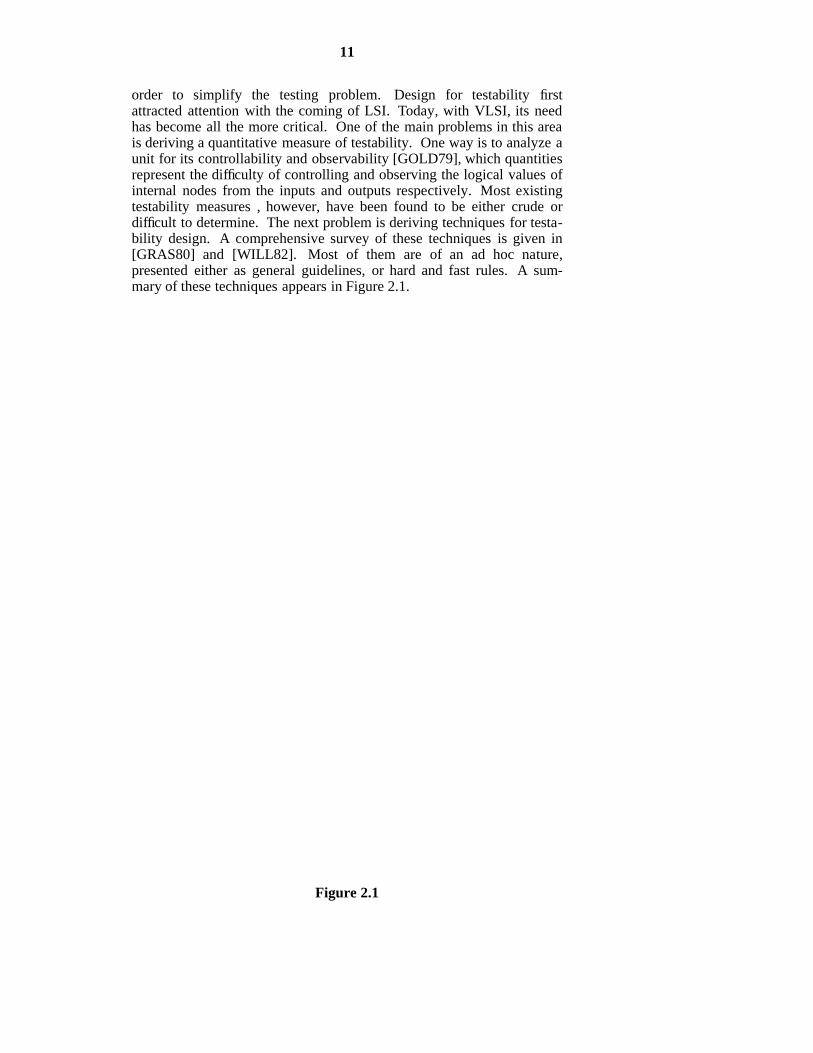
order to simplify the testing problem. Design for testability firstattracted attention with the coming of LSI. Today, with VLSI, its needhas become all the more critical. One of the main problems in this areais deriving a quantitative measure of testability. One way is to analyze aunit for its controllability and observability [GOLD79], which quantitiesrepresent the difficulty of controlling and observing the logical values ofinternal nodes from the inputs and outputs respectively. Most existingtestability measures , however, have been found to be either crude ordifficult to determine. The next problem is deriving techniques for testa-bility design. A comprehensive survey of these techniques is given in[GRAS80] and [WILL82]. Most of them are of an ad hoc nature,presented either as general guidelines, or hard and fast rules. A sum-mary of these techniques appears in Figure 2.1.

Figure 2.1

-- --

12

2.1.4.2 Design VerificationThe central issue here is proving the correctness of a design. Does adesign do what it is supposed to do? In other words, we are dealing withthe testing for design faults. The purpose of design verification is quiteclear. Design faults must be eliminated, as far as possible, before thehardware is constructed, and before prototype tests begin. The increas-ing cost of implementing engineering changes given LSI/VLSI hardwarehas enhanced the need for design verification.

Compared to physical faults, design faults are more subtle and seri-ous and can be extremely difficult to handle. Hence, the techniquesdeveloped for physical faults cannot be effectively extended to designfaults. To date, very little effort has been devoted to formalizing designverification. Designs are still mostly checked by ad hoc means, like faultsimulation and prototype checkout.

Like other disciplines, design verification too has not been sparedthe impact of LSI/VLSI. Some of these influences are listed below.

Ratification or matching the design specification was accomplished inthe pre-LSI era by gate-level simulation. This may no longer besufficient. The simulations need to be more detailed, and they need to bedone at higher levels, like the functional and behavioral levels. Also,techniques are required for determining the following:

(1) Stopping rules for simulation.(2) The extent of design faults removed.(3) A quantitative measure for the correctness or quality of the final

design.

Validation. In the pre-LSI days, this was restricted to the testing ofhardware on the test floor. Moreover, the testing process was not formal-ized or systematic, and hence lacked thoroughness and rigor. Today,validation mainly involves testing the equivalence of two designdescriptions. The descriptions may be at different levels. Thus, beforebeing compared, they need to be translated to a common level. Forexample, one can construct symbolic execution tree models of the designdescriptions to be compared.

Timing Analysis. In the past, it was sufficient to analyze only single "crit-ical" paths. The technology rules of LSI/VLSI are so complex that theidentification of these critical paths has become extremely difficult. Sta-tistical timing analysis methods need to be investigated, in order to copewith the tremendous densities and wide range of tolerances imposed byLSI/VLSI.

Finally, research has also started in developing design techniquesto alleviate the need for, and/or facilitate, the design verification process.

3. COMPLEXITY AND NONDETERMINISM

3.1 ComplexityBy the complexity of an algorithm, we mean the amount of computertime and memory space needed to run this algorithm. These two quanti-ties will be referred to respectively as the time and space complexities ofthe algorithm. To illustrate, consider procedure MADD (Algorithm 3.1):it is an algorithm to add two mxn matrices together.

-- --

13

line procedure MADD(A,B,C,m,n)compute C=A+B

1 declare A(m,n),B(m,n),C(m,n)2 for i ← 1 to m do3 for j ← 1 to n do4 C(i,j) ← A(i,j)+B(i,j)5 endfor6 endfor7 end MADD

Algorithm 3.1 Matrix addition.

The time needed to run this algorithm on a computer comprisestwo components: the time to compile the algorithm and the time to exe-cute it. The first of these two components depends on the compiler andthe computer being used. This time is, however, independent of theactual values of n and m. The execution time, in addition to being depen-dent on the compiler and the computer used, depends on the values of mand n. It takes more time to add larger matrices.

Since the actual time requirements of an algorithm are verymachine-dependent, the theoretical analysis of the time complexity of analgorithm is restricted to determining the number of steps needed by thealgorithm. This step count is obtained as a function of certain parametersthat characterize the input and output. Some examples of often-usedparameters are: number of inputs; number of outputs; magnitude ofinputs and outputs; etc.

In the case of our matrix addition example, the number of rows mand the number of columns n are reasonable parameters to use. Ifinstruction 4 of procedure MADD is assigned a step count of 1 per exe-cution, then its total contribution to the step count of the algorithm is mn,as this instruction is executed mn times. [SAHN80, Chapter 6] discussesstep count analysis in greater detail. Since the notion of a step is some-what inexact, one often does not strive to obtain an exact step count foran algorithm. Rather, asymptotic bounds on the step count are obtained.Asymptotic analysis uses the notation Ο, Ω, Θ and o. These are definedbelow.

Definition: [Asymptotic Notation] f(n) = Ο(g(n)) (read as "f of n is bigoh of g of n") iff there exist positive constants c and n0 such thatf(n)≤cg(n) for all n, n≥n0 . f(n) = Ω(g(n)) (read as "f of n is omega of g ofn") iff there exist positive constants c and n0 such that f(n)≥cg(n) for alln, n≥n0. f(n) is Θ(g(n)) (read as "f of n is theta of g of n") iff there existpositive constants c 1 , c 2, and n0 such that c 1g(n)≤f(n)≤c 2g(n) for all n,n≥n0. f(n) = o(g(n)) (read as "f of n is little o of g of n") iff

n →∞lim f (n)/g (n)

= 1.The definitions of Ο, Ω, Θ, and o are easily extended to include

functions of more than one variable. For example, f(n,m) = Ο(g(n,m)) iffthere exist positive constants c, n0, and m0 such that f(n,m)≤cg(n,m) forall n≥n0 and all m≥m0.

Example 3.1: 3n+2=Ο(n) as 3n+2≤4n for all n, n≥2. 3n+2=Ω(n) and3n+2=Θ(n). 6*2n+n2=Ο(2n). 3n=Ο(n2). 3n=o(3n) and 3n=Ο(n3).

As illustrated by the previous example, the statement f(n)=Ο(g(n))only states that g(n) is an upper bound on the value of f(n) for all n, n≥n0 .

-- --

14

It doesn’t say anything about how good this bound is. Notice that ifn=Ο(n), n=Ο(n2), n=Ο(n2.5), etc. In order to be informative, g(n) shouldbe as small a function of n as one can come up with such thatf(n)=Ο(g(n)). So, while we shall often say that 3n+3=Ο(n), we shallalmost never say that 3n+3=Ο(n2).

As in the case of the "big oh" notation, there are several functionsg(n) for which f(n)=Ω(g(n)). g(n) is only a lower bound on f(n). Thetheta notation is more precise than both the "big oh" and omega nota-tions. The following theorem obtains a very useful result about the orderof f(n) when f(n) is a polynomial in n.

Theorem 3.1: Let f(n)=amnm+am −1nm −1+ . . . +a0, am ≠ 0.(a) f(n) = O(nm)

(b) f(n) = Ω(nm)(c) f(n) = Θ(nm)(d) f(n) = o(amnm)

Asymptotic analysis may also be used for space complexity.While asymptotic analysis does not tell us how many seconds an

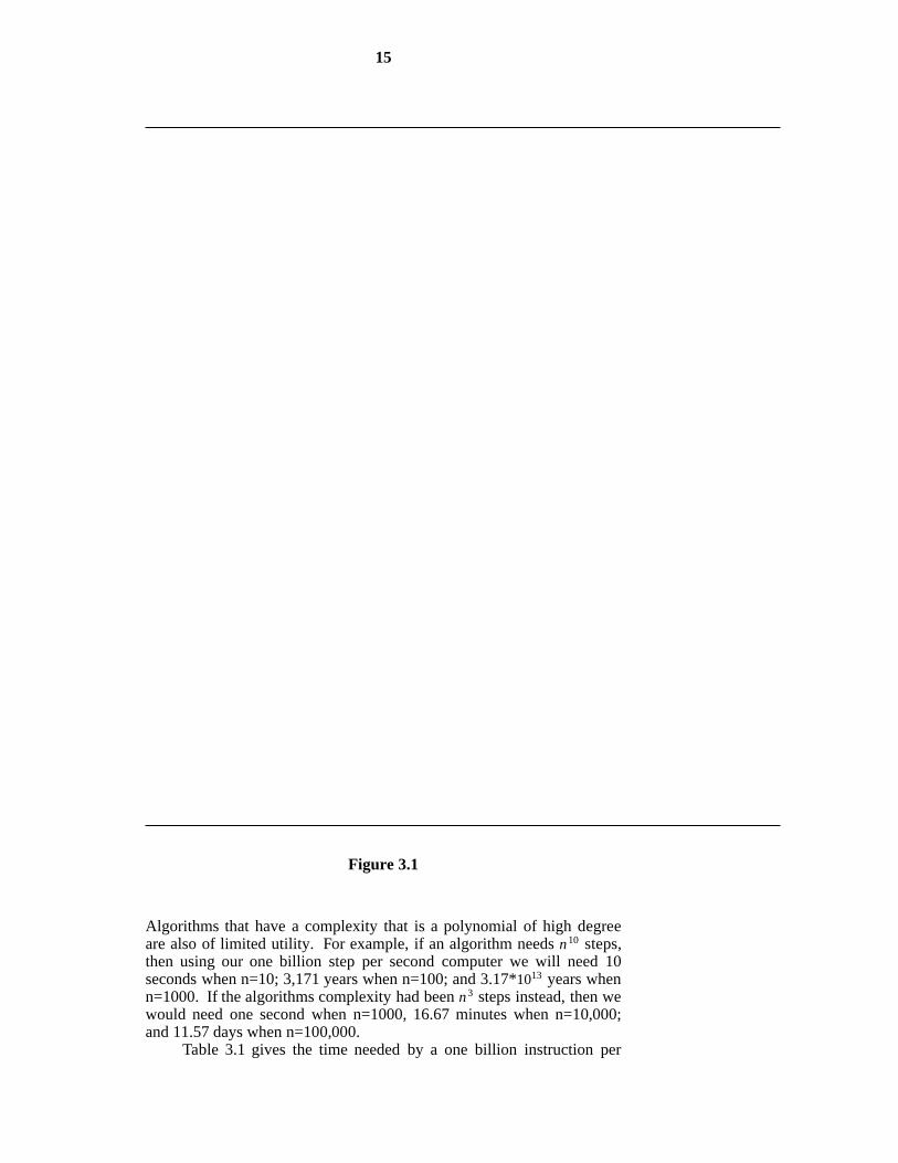
algorithm will run for or how many words of memory it will require, itdoes characterize the growth rate of the complexity (see Figure 3.1).So, if procedure MADD takes 2 milliseconds (ms) on a problem withm=100 and n=20, then we expect it to take about 16ms when mn=16000(the complexity of MADD is Θ(mn)). For sufficiently large values of n, aΘ(n2) algorithm will be faster than a Θ(n3) algorithm.

We have seen that the time complexity of an algorithm is generallysome function of the instance characteristics. This function is very use-ful in determining how the time requirements vary as the instancecharacteristics change. The complexity function may also be used tocompare two algorithms A and B that perform the same task. Assumethat algorithm A has complexity Θ(n) and algorithm B is of complexityΘ(n2). We can assert that algorithm A is faster than algorithm B for"sufficiently large" n. To see the validity of this assertion, observe thatthe actual computing time of A is bounded from above by n for someconstant c and for all n, n≥n1 while that of B is bounded from below bydn2 for some constant d and all n, n≥n2. Since cn≤dn2 for n≥c/d, algo-rithm A is faster than algorithm B whenever n≥maxn1, n2, c/d. Oneshould always be cautiously aware of the presence of the phrase"sufficiently large" in the assertion of the preceding discussion. Whendeciding which of the two algorithms to use, we must know whether then we are dealing with is in fact "sufficiently large". If algorithm A actu-ally runs in 106n milliseconds while algorithm B runs in n2 millisecondsand if we always have n≤106 , then algorithm B is the one to use. To geta feel for how the various functions grow with n, you are advised tostudy Figure 3.1 very closely. As is evident from the figure, the function2n grows very rapidly with n. In fact, if an algorithm needs 2n steps forexecution, then when n=40 the number of steps needed is approximately1.1*1012 . On a computer performing one billion steps per second, thiswould require about 18.3 minutes. If n=50, the same algorithm wouldrun for about 13 days on this computer. When n=60, about 36.56 yearswill be required to execute the algorithm and when n=100, about 4*1013

years will be needed. So, we may conclude that the utility of algorithmswith exponential complexity is limited to small n (typically n≤40).

-- --

15

Figure 3.1

Algorithms that have a complexity that is a polynomial of high degreeare also of limited utility. For example, if an algorithm needs n10 steps,then using our one billion step per second computer we will need 10seconds when n=10; 3,171 years when n=100; and 3.17*1013 years whenn=1000. If the algorithms complexity had been n3 steps instead, then wewould need one second when n=1000, 16.67 minutes when n=10,000;and 11.57 days when n=100,000.

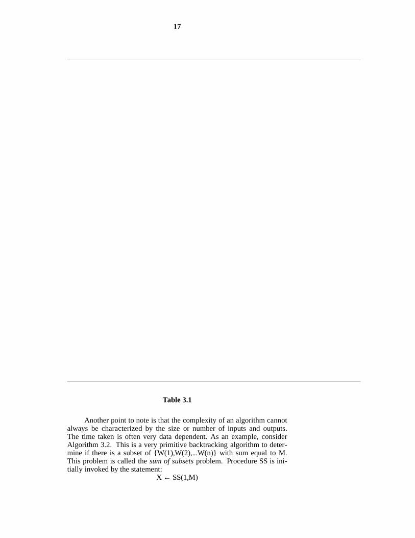
Table 3.1 gives the time needed by a one billion instruction per

-- --

16

second computer to execute a program of complexity f(n) instructions.One should note that currently only the fastest computers can executeabout one billion instructions per second. From a practical standpoint, itis evident that for reasonably large n (say n>100) only algorithms ofsmall complexity (such as n, nlogn, n2, n3, etc.) are feasible. Further,this is the case even if one could build a computer capable of executing1012 instructions per second. In this case, the computing times of Table3.1 would decrease by a factor of 1000. Now, when n = 100 it wouldtake 3.17 years to execute n10 instructions, and 4*1010 years to execute2n instructions.

-- --

17

Table 3.1

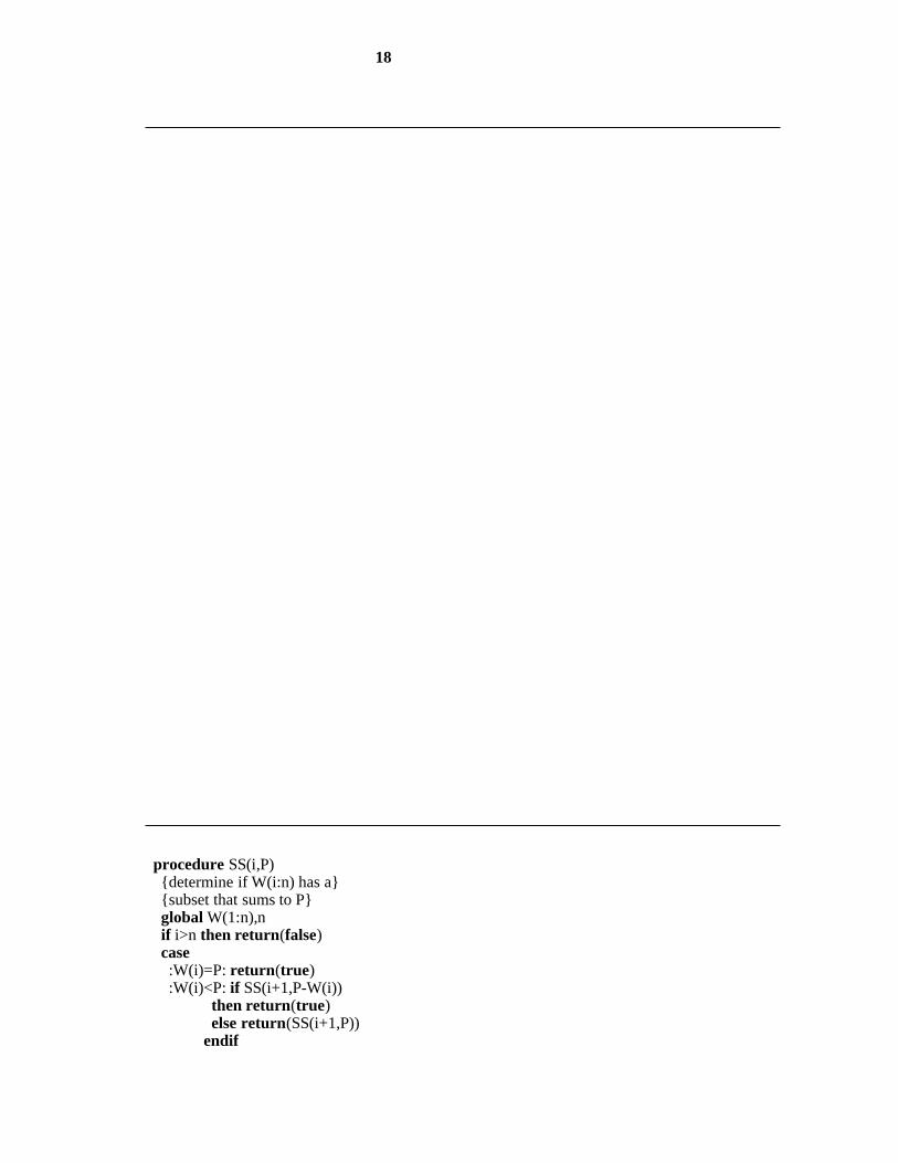
Another point to note is that the complexity of an algorithm cannotalways be characterized by the size or number of inputs and outputs.The time taken is often very data dependent. As an example, considerAlgorithm 3.2. This is a very primitive backtracking algorithm to deter-mine if there is a subset of W(1),W(2),...W(n) with sum equal to M.This problem is called the sum of subsets problem. Procedure SS is ini-tially invoked by the statement:

X ← SS(1,M)

-- --

18

procedure SS(i,P)determine if W(i:n) has asubset that sums to Pglobal W(1:n),nif i>n then return(false)case:W(i)=P: return(true):W(i)<P: if SS(i+1,P-W(i))

then return(true)else return(SS(i+1,P))

endif

-- --

19

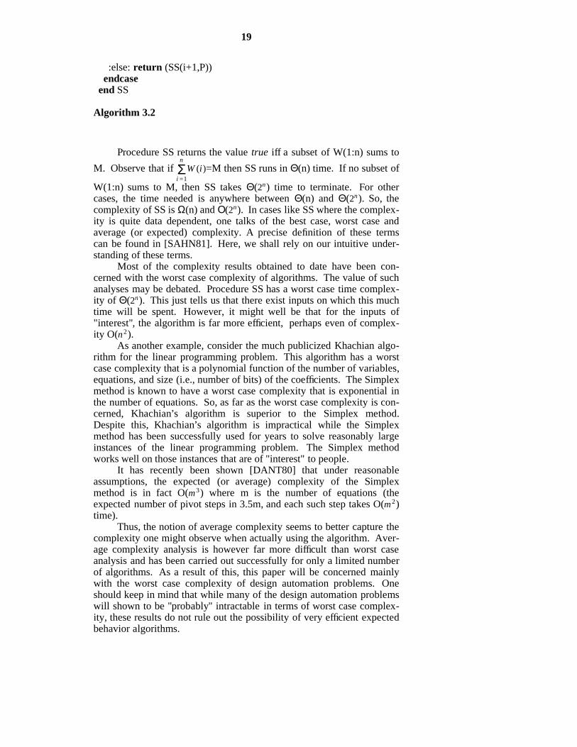
:else: return (SS(i+1,P))endcase

end SS

Algorithm 3.2

Procedure SS returns the value true iff a subset of W(1:n) sums to

M. Observe that ifi =1Σn

W (i)=M then SS runs in Θ(n) time. If no subset of

W(1:n) sums to M, then SS takes Θ(2n) time to terminate. For othercases, the time needed is anywhere between Θ(n) and Θ(2n). So, thecomplexity of SS is Ω(n) and Ο(2n). In cases like SS where the complex-ity is quite data dependent, one talks of the best case, worst case andaverage (or expected) complexity. A precise definition of these termscan be found in [SAHN81]. Here, we shall rely on our intuitive under-standing of these terms.

Most of the complexity results obtained to date have been con-cerned with the worst case complexity of algorithms. The value of suchanalyses may be debated. Procedure SS has a worst case time complex-ity of Θ(2n). This just tells us that there exist inputs on which this muchtime will be spent. However, it might well be that for the inputs of"interest", the algorithm is far more efficient, perhaps even of complex-ity O(n2).

As another example, consider the much publicized Khachian algo-rithm for the linear programming problem. This algorithm has a worstcase complexity that is a polynomial function of the number of variables,equations, and size (i.e., number of bits) of the coefficients. The Simplexmethod is known to have a worst case complexity that is exponential inthe number of equations. So, as far as the worst case complexity is con-cerned, Khachian’s algorithm is superior to the Simplex method.Despite this, Khachian’s algorithm is impractical while the Simplexmethod has been successfully used for years to solve reasonably largeinstances of the linear programming problem. The Simplex methodworks well on those instances that are of "interest" to people.

It has recently been shown [DANT80] that under reasonableassumptions, the expected (or average) complexity of the Simplexmethod is in fact O(m3) where m is the number of equations (theexpected number of pivot steps in 3.5m, and each such step takes O(m2)time).

Thus, the notion of average complexity seems to better capture thecomplexity one might observe when actually using the algorithm. Aver-age complexity analysis is however far more difficult than worst caseanalysis and has been carried out successfully for only a limited numberof algorithms. As a result of this, this paper will be concerned mainlywith the worst case complexity of design automation problems. Oneshould keep in mind that while many of the design automation problemswill shown to be "probably" intractable in terms of worst case complex-ity, these results do not rule out the possibility of very efficient expectedbehavior algorithms.

-- --

20

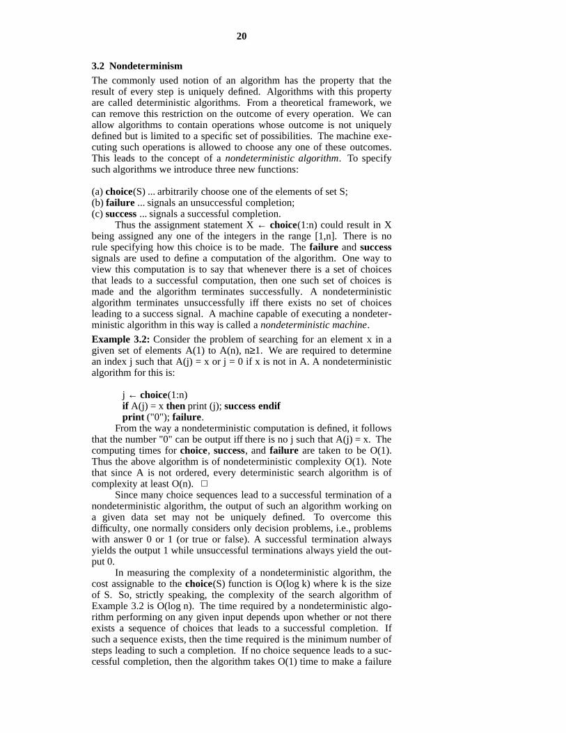
3.2 NondeterminismThe commonly used notion of an algorithm has the property that theresult of every step is uniquely defined. Algorithms with this propertyare called deterministic algorithms. From a theoretical framework, wecan remove this restriction on the outcome of every operation. We canallow algorithms to contain operations whose outcome is not uniquelydefined but is limited to a specific set of possibilities. The machine exe-cuting such operations is allowed to choose any one of these outcomes.This leads to the concept of a nondeterministic algorithm. To specifysuch algorithms we introduce three new functions:

(a) choice(S) ... arbitrarily choose one of the elements of set S;(b) failure ... signals an unsuccessful completion;(c) success ... signals a successful completion.

Thus the assignment statement X ← choice(1:n) could result in Xbeing assigned any one of the integers in the range [1,n]. There is norule specifying how this choice is to be made. The failure and successsignals are used to define a computation of the algorithm. One way toview this computation is to say that whenever there is a set of choicesthat leads to a successful computation, then one such set of choices ismade and the algorithm terminates successfully. A nondeterministicalgorithm terminates unsuccessfully iff there exists no set of choicesleading to a success signal. A machine capable of executing a nondeter-ministic algorithm in this way is called a nondeterministic machine.

Example 3.2: Consider the problem of searching for an element x in agiven set of elements A(1) to A(n), n≥1. We are required to determinean index j such that A(j) = x or j = 0 if x is not in A. A nondeterministicalgorithm for this is:

j ← choice(1:n)if A(j) = x then print (j); success endifprint ("0"); failure.

From the way a nondeterministic computation is defined, it followsthat the number "0" can be output iff there is no j such that A(j) = x. Thecomputing times for choice, success, and failure are taken to be O(1).Thus the above algorithm is of nondeterministic complexity O(1). Notethat since A is not ordered, every deterministic search algorithm is ofcomplexity at least O(n).

Since many choice sequences lead to a successful termination of anondeterministic algorithm, the output of such an algorithm working ona given data set may not be uniquely defined. To overcome thisdifficulty, one normally considers only decision problems, i.e., problemswith answer 0 or 1 (or true or false). A successful termination alwaysyields the output 1 while unsuccessful terminations always yield the out-put 0.

In measuring the complexity of a nondeterministic algorithm, thecost assignable to the choice(S) function is O(log k) where k is the sizeof S. So, strictly speaking, the complexity of the search algorithm ofExample 3.2 is O(log n). The time required by a nondeterministic algo-rithm performing on any given input depends upon whether or not thereexists a sequence of choices that leads to a successful completion. Ifsuch a sequence exists, then the time required is the minimum number ofsteps leading to such a completion. If no choice sequence leads to a suc-cessful completion, then the algorithm takes O(1) time to make a failure

-- --

21

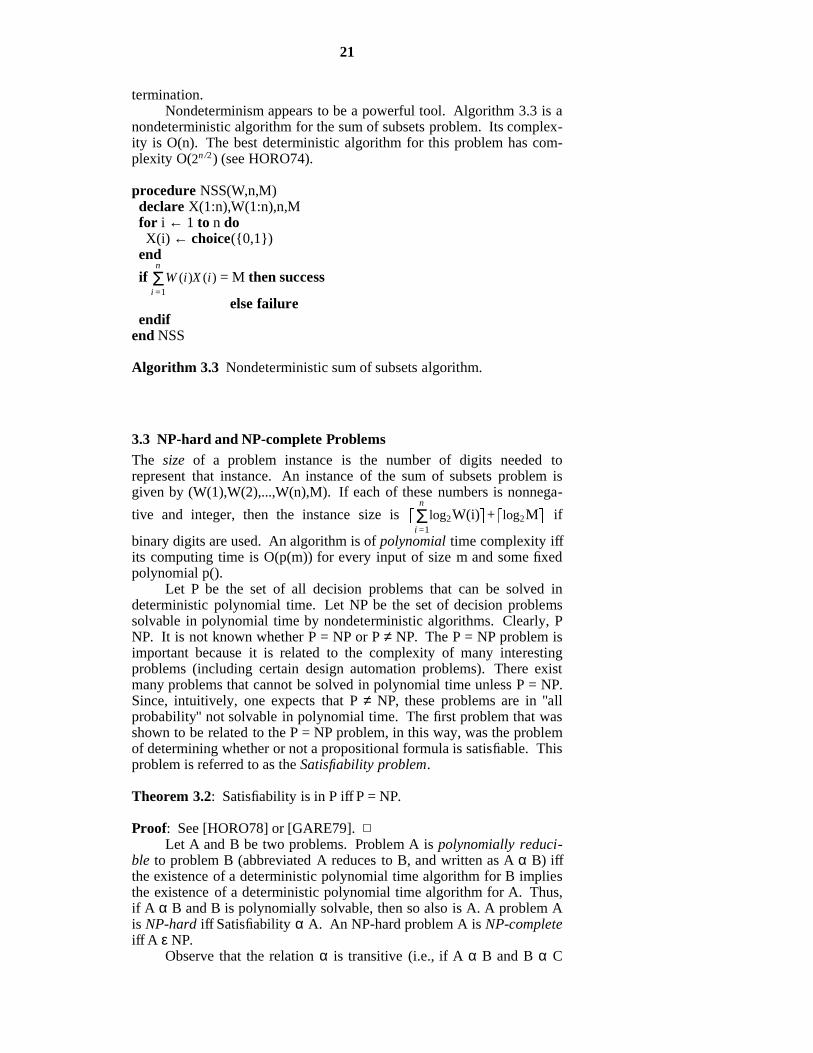
termination.Nondeterminism appears to be a powerful tool. Algorithm 3.3 is a

nondeterministic algorithm for the sum of subsets problem. Its complex-ity is O(n). The best deterministic algorithm for this problem has com-plexity O(2n /2) (see HORO74).

procedure NSS(W,n,M)declare X(1:n),W(1:n),n,Mfor i ← 1 to n doX(i) ← choice(0,1)

end

ifi =1Σn

W (i)X (i) = M then success

else failureendif

end NSS

Algorithm 3.3 Nondeterministic sum of subsets algorithm.

3.3 NP-hard and NP-complete ProblemsThe size of a problem instance is the number of digits needed torepresent that instance. An instance of the sum of subsets problem isgiven by (W(1),W(2),...,W(n),M). If each of these numbers is nonnega-

tive and integer, then the instance size is

i =1Σn

log2W(i) +log2M if

binary digits are used. An algorithm is of polynomial time complexity iffits computing time is O(p(m)) for every input of size m and some fixedpolynomial p().

Let P be the set of all decision problems that can be solved indeterministic polynomial time. Let NP be the set of decision problemssolvable in polynomial time by nondeterministic algorithms. Clearly, PNP. It is not known whether P = NP or P ≠ NP. The P = NP problem isimportant because it is related to the complexity of many interestingproblems (including certain design automation problems). There existmany problems that cannot be solved in polynomial time unless P = NP.Since, intuitively, one expects that P ≠ NP, these problems are in "allprobability" not solvable in polynomial time. The first problem that wasshown to be related to the P = NP problem, in this way, was the problemof determining whether or not a propositional formula is satisfiable. Thisproblem is referred to as the Satisfiability problem.

Theorem 3.2: Satisfiability is in P iff P = NP.

Proof: See [HORO78] or [GARE79].Let A and B be two problems. Problem A is polynomially reduci-

ble to problem B (abbreviated A reduces to B, and written as A α B) iffthe existence of a deterministic polynomial time algorithm for B impliesthe existence of a deterministic polynomial time algorithm for A. Thus,if A α B and B is polynomially solvable, then so also is A. A problem Ais NP-hard iff Satisfiability α A. An NP-hard problem A is NP-completeiff A ε NP.

Observe that the relation α is transitive (i.e., if A α B and B α C

-- --

22

then A α C). Consequently, if A α B and Satisfiability α A then B isNP-hard. So, to show that any problem B is NP-hard, we need merelyshow that A α B where A is any known NP-hard problem. Some of theknown NP-hard problems are:

NP1: Euclidean Steiner Tree [GARE77]Input: A set X = (xi,yi)|1≤i≤n of points.Output: A finite set Y = (ai,bi)|1≤i≤m of points such that the minimumspanning tree for XY is of minimum total length over all choices for Y.The distance between two points (t,u) and (v,w) is [(t −v)2+(u −w)2].

NP2: Manhattan Steiner Tree [GARE77]Input: Same as in NP1.Output: Same as in NP1, except that the distance between two points istaken to be |t-v|+|u-w|.

NP3: Euclidean Traveling Salesman [GARE76b]Input: Same as in NP1.Output: A minimum length tour going through each point in X. TheEuclidan distance measure is used.

NP4: Euclidean Path Traveling Salesman [PAPA77](also called Euclidean Hamiltonian Path)

Input: Same is in NP1.Output: A minimum length path that visits all points in X exactly once.The Euclidean distance measure is used.

NP5: Manhattan Traveling Salesman [GARE76b]Input: Same as in NP3.Output: Same as in NP3, except that the Manhattan distance measure isused.

NP6: Manhattan Path Traveling Salesman [PAPA77](also called Manhattan Hamiltonian Path)

Input: Same as in NP1.Output: Same as in NP4, except that the Manhattan distance measure isused.

NP7: Chromatic Number I [EHRL76]Input: A graph G which is the intersection graph for straight line seg-ments in the plane.Output: The minimum number of colors needed to color G.

NP8: Chromatic Number II [EHRL76]Input: Same as in NP5.Output: ’Yes’ if G is 3-colorable and ’No’ otherwise.

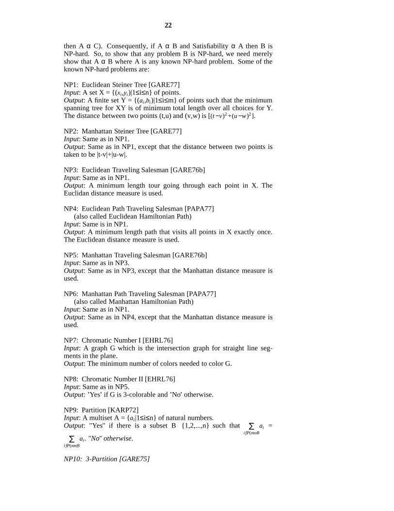
NP9: Partition [KARP72]Input: A multiset A = ai|1≤i≤n of natural numbers.Output: "Yes" if there is a subset B 1,2,...,n such that

i fP(moBΣ ai =

i fP(nmBΣ ai. "No" otherwise.

NP10: 3-Partition [GARE75]

-- --

23

Input: A multiset A = ai|1≤i≤3m of natural numbers, and a bound B,such that

(i)aifP(moA

Σ ai = mB

(ii) B/4 < ai < B/2 for 1≤i≤3mOutput: "Yes" if A can be partitioned into m disjoint sets A1 ,A2 , . . . Am

such that, for 1≤i≤m,ajεAi

Σ aj = B; "No" otherwise.

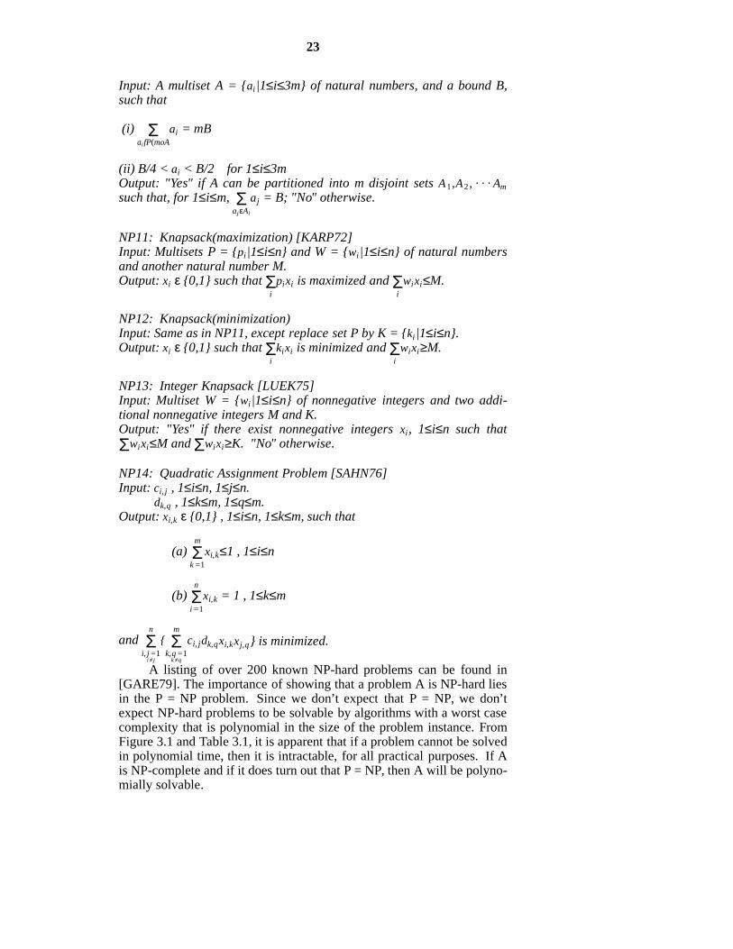
NP11: Knapsack(maximization) [KARP72]Input: Multisets P = pi|1≤i≤n and W = wi|1≤i≤n of natural numbersand another natural number M.Output: xi ε 0,1 such that

iΣpixi is maximized and

iΣwixi≤M.

NP12: Knapsack(minimization)Input: Same as in NP11, except replace set P by K = ki|1≤i≤n.Output: xi ε 0,1 such that

iΣkixi is minimized and

iΣwixi≥M.

NP13: Integer Knapsack [LUEK75]Input: Multiset W = wi|1≤i≤n of nonnegative integers and two addi-tional nonnegative integers M and K.Output: "Yes" if there exist nonnegative integers xi, 1≤i≤n such thatΣwixi≤M and Σwixi≥K. "No" otherwise.

NP14: Quadratic Assignment Problem [SAHN76]Input: ci, j , 1≤i≤n, 1≤j≤n.

dk,q , 1≤k≤m, 1≤q≤m.Output: xi,k ε 0,1 , 1≤i≤n, 1≤k≤m, such that

(a)k =1Σm

xi,k≤1 , 1≤i≤n

(b)i =1Σn

xi,k = 1 , 1≤k≤m

andi ≠j

i, j =1Σn

k ≠qk,q =1Σm

ci, jdk,qxi,kxj,q is minimized.

A listing of over 200 known NP-hard problems can be found in[GARE79]. The importance of showing that a problem A is NP-hard liesin the P = NP problem. Since we don’t expect that P = NP, we don’texpect NP-hard problems to be solvable by algorithms with a worst casecomplexity that is polynomial in the size of the problem instance. FromFigure 3.1 and Table 3.1, it is apparent that if a problem cannot be solvedin polynomial time, then it is intractable, for all practical purposes. If Ais NP-complete and if it does turn out that P = NP, then A will be polyno-mially solvable.

-- --

24

4. COMPLEXITY OF DESIGN AUTOMATION PROBLEMSIn Section 4.1 we illustrate how one goes about showing that a problemis NP-hard or NP-complete. We consider three examples from thedesign automation area. Over thirty design automation problems aredescribed in Section 4.2. With each problem, a discussion of its com-plexity is included.

4.1 Showing Problems NP-hard and NP-complete

4.1.1 Circuit RealizationIn this problem, we are given a set of r modules. Associated withmodule i is a cost ci, 1≤i≤r. Module i contains mij gates of type j, 1≤j≤n.We are required to realize a circuit C with gate requirements(b1,b2,...,bn), i.e., circuit C consists of bj gates of type j. (x 1,...,xr) real-izes circuit C iff

i =1Σr

mijxi≥ bj, 1≤j≤n

and xi is a natural number, 1≤i≤r.

The cost of the realization (x 1,...,xr) isi =1Σr

cixi. We are interested in

obtaining a minimum cost realization of C.

Theorem 4.1: The circuit realization problem is NP-hard.

Proof: From Section 3.2, we see that it is sufficient to show that Q α cir-cuit realization, where Q is any known NP-hard problem. We shall use Q= NP13 = integer knapsack (Section 3.2).

Let (w1,w2 ,...,wp), M, and K be any instance of the integer knap-sack problem. Construct the following circuit realization instance:

n = 1 ; b1 = K ; r = p ; mi, 1 = wi, 1≤i≤p ; ci = wi, 1≤i≤pClearly, the least cost realization of the above circuit instance has a

cost at most M iff the corresponding integer knapsack instance hasanswer "yes". So if the circuit realization problem is polynomially solv-able, then so also is NP13. But NP13 is NP-hard. So, circuit realizationis also NP-hard.

In order to show that an NP-hard problem Q is NP-complete, weneed to show that it is in NP. Only decision problems (i.e., problems forwhich the output is "yes" or "no") can be NP-complete. So, the circuitrealization problem cannot be NP-complete. However, we may formu-late a decision version of the circuit realization problem : Is there a real-ization with cost no more than S? The proof provided in Theorem 4.1 isvalid for this version of the problem too. Also, there is a nondeterminis-tic polynomial time algorithm for this decision problem (Algorithm 4.1).So, the decision version of the circuit realization problem is NP-complete.

-- --

25

procedure CKT(b,S,m,r,n,c)Bs there a circuit realization with cost ≤ S?declare r, n, c(r), m(r,n), b(n), S, x(r)q ←

jmax b(j)

for i ← 1 to r do obtain xis nondeterministicallyx(i) ← choice(0:q)

endforfor i←1 to n do check feasibility

ifj=1Σr

m(j,i)∗x(i) < b(i) then failure endif

endfor

ifi =1Σr

c(i)x(i) > S then failure

else successend CKT

Algorithm 4.1

4.1.2 Euclidean Layering ProblemA wire to be laid out may be defined by the two end points (x,y) and(u,v) of the wire. (x,y) and (u,v) are the coordinates of the two endpoints. In a Euclidean layout, the wire runs along a straight line from(x,y) to (u,v). Figure 4.1(a) shows some wires laid out in a Euclideanmanner. Let W = [(ui,vi),(xi,yi)] | 1≤i≤n be a set of n wires. In theEuclidean layering problem, we are required to partition W into aminimum number of disjoint sets W 1,W 2,..., Wk such that no two wires inany set Wi cross. Figure 4.1(b) gives a partitioning of the wires of Figure4.1(a) that satisfies this requirement. The wires in W1 and W2 can nowbe routed in separate layers.

-- --

26

Figure 4.1

Theorem 4.2: The Euclidean layering problem is NP-hard.

Proof: We shall show that the known NP-hard problem NP7 (ChromaticNumber I) reduces to the Euclidean layering problem. Let G=(V,E) beany intersection graph for straight line segments in the plane. Let W bethe corresponding set of straight line segments. Note that W=V as V hasone vertex for each line segment in W. Also, (i,j) is an edge of G iff theline segments corresponding to vertices i and j intersect in Euclideanspace. From any partitioning W 1,W 2,... of W such that no two line seg-ments of any partition intersect, we can obtain a coloring of G. Vertex iis assigned the color j iff the line segment corresponding to vertex i is inthe partition Wj. No adjacent vertices in G will be assigned the samecolor as the line segments corresponding to adjacent vertices intersectand so must be in different partitions. Furthermore, if G can be coloredwith k colors, then W can be partitioned into W1 ,...,Wk.

Hence, G can be colored with k colors iff W can be partitioned intok disjoint sets, no set containing two intersecting segments. So, if wecould solve the Euclidean layering problem in polynomial time, then wecould solve the chromatic number problem NP7 in polynomial time byfirst obtaining W as above and then using the polynomial time algorithmto minimally partition W. From the partition, a coloring of G can beobtained. Since NP7 is NP-hard, it follows that the Euclidean layeringproblem is also NP-hard.

The above equivalence between NP7 and the Euclidean layeringproblem was pointed out by Akers [BREU72].

A decision version of the Euclidean layering problem would takethe form: Can W be partitioned into ≤ k partitions such that no partitioncontains two wires that intersect? The proof of Theorem 4.2 shows thatthis decision problem is NP-hard. Procedure ELP (Algorithm 4.2) is anondeterministic polynomial time algorithm for this problem. Hence,the decision version of the Euclidean layering problem is NP-complete.

-- --

27

procedure ELP(W,n,k)n = Wwire set W, integer n,k;L(i) ← 0, 1≤i≤kfor i←1 to n do assign wires to layers

j ← choice(1:k)L(j) ← L(j) ∪ [(ui,vi),(xi,yi)]

endforfor i←1 to k do check for intersections

if two wires in L(i) intersect then failureendif

endforsuccess

end ELP

Algorithm 4.2

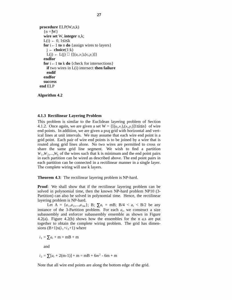
4.1.3 Rectilinear Layering ProblemThis problem is similar to the Euclidean layering problem of Section4.1.2. Once again, we are given a set W = [(ui,vi),(xi,yi)]1≤i≤n of wireend points. In addition, we are given a pxq grid with horizontal and vert-ical lines at unit intervals. We may assume that each wire end point is agrid point. Each pair of wire end points is to be joined by a wire that isrouted along grid lines alone. No two wires are permitted to cross orshare the same grid line segment. We wish to find a partitionW 1,W 2,...,Wk of the wires such that k is minimum and the end point pairsin each partition can be wired as described above. The end point pairs ineach partition can be connected in a rectilinear manner in a single layer.The complete wiring will use k layers.

Theorem 4.3: The rectilinear layering problem is NP-hard.

Proof: We shall show that if the rectilinear layering problem can besolved in polynomial time, then the known NP-hard problem NP10 (3-Partition) can also be solved in polynomial time. Hence, the rectilinearlayering problem is NP-hard.

Let A = a1 ,a2,...,a3m; B; Σai = mB; B/4 < ai < B/2 be anyinstance of the 3-Partition problem. For each ai, we construct a sizesubassembly and enforcer subassembly ensemble as shown in Figure4.2(a). Figure 4.2(b) shows how the ensembles for the n ais are puttogether to obtain the complete wiring problem. The grid has dimen-sions (B+1)x(i1+i2+1) where

i1 = Σai + m = mB + m

and

i2 = Σ[ai + 2(m-1)] + m = mB + 6m2 - 6m + m

Note that all wire end points are along the bottom edge of the grid.

-- --

28

Figure 4.2

The valve assembly shown in Figure 4.2(b) is similar to theenforcer subassembly except that it contains m wires instead of m-1. Asis evident, no two wires of the valve assembly can be routed in the samelayer. Hence, at least m layers are needed to wire the valve.

An examination of the ensemble for each ai reveals that:

(i) no 2 wires in the enforcer subassembly can be routed on the samelayer, obviously.

(ii) a wire from the size subassembly cannot be routed on the samelayer with a wire from the enforcer subassembly.

(iii) all wires in a size subassembly can be routed on the same layer.

Therefore, at least m layers are required to route each ensemble. Hence,the rectilinear layering problem defined by Figure 4.2(b) needs at least mlayers.

If the 3-Partition instance has a 3-Partition A1, A2,...,Am, then onlym layers are needed by Figure 4.2(b). In layer i, we wire the sizesubassemblies for the three ajs in Ai as well as one wire of the valve andone wire from each of the 3m-3 enforcer subassemblies corresponding tothe 3m-3 ajs not in Ai.

On the other hand, if Figure 4.2(b) can be wired in m layers, thenthere is a 3-Partition of the ais. Since no layer may contain more than 1wire from the valve, each layer contains exactly B wires from the sizeensembles. If a wire from the size ensemble for ai is in layer j, then all ai

wires from this ensemble must be in this layer. To see this, observe thatthe remaining m-1 layers must each contain exactly 1 wire from ai’senforcer subassembly and so can contain no wires from the sizesubassembly. Hence, each layer must contain exactly three size ensem-bles. The 3-Partition is therefore Ai= j the size subassembly for j is inlayer i.

So, Figure 4.2(b) can be wired in m layers iff the 3-Partitioninstance has answer "yes". Hence, the rectilinear layering problem isNP-hard.

As in the case of the problems considered in Sections 4.1.1 and4.1.2, we may define a decision version of the rectilinear layering prob-lem and show that this version is NP-complete.

4.2 Mathematical Formulation and Complexity of Design Automa-tion Problems

4.2.1 Implementation Problems

IP1: Function RealizationInput: A Boolean function B and a set of component types C1 ,C2,...,Ck.Ci realizes the Boolean function Fi.Output: A circuit made up of component types C1 ,C2,...,Ck realizing Band using the minimum total number of components.Complexity: NP-hard. The proof can be found in [IBAR75a], where IP1is called P6.

IP2: Circuit Correctness

-- --

29

Input: A Boolean function B and a circuit C.Output: "yes" if C realizes B and "no" otherwise.Complexity: NP-hard. The proof can be found in [IBAR75a], where it iscalled P5. It is shown that tautology reduces to P5 (IP2).

IP3: Circuit RealizationInput: Circuit requirements (b1,b2 ,...,bn) with the interpretation that bi

gates of type i are needed to realize the circuit; modules 1,2,...,r withcomposition mij, where module i has mij gates of type j; module costs ci,where ci is the cost of one unit of module i.Output: Nonnegative integers x 1,x 2,...,xn such that

iΣmijxi ≥ bj, i≤j≤n and

iΣcixi is minimized.

Complexity: NP-hard. See Section 4.1.1.

IP4: Construction of a Minimum Cost Standard Library of ReplaceableModulesInput: A set C1 ,C2,...,Cn of logic circuits such that circuit Ci containsyij circuits of type j, 1≤j≤r; and a limit, p, on the number of circuits thatcan be put into a module.Output: A set M=m1,m2,...,mk of module types, with module mi con-taining aij circuits of type j, such that:

(i)j

Σ aij ≤ p, 1 ≤ i ≤ k ;

(ii) Σ xij ajq ≥ yiq, 1 ≤ i ≤ n and 1 ≤ q ≤ r;

xij = smallest number of modules mj needed in implementing Ci.

(iii)iΣ

jΣxij is minimum over all choices of M.

Complexity: NP-hard. Partition (NP9) reduces to IP4 as follows. LetA=a1 ,a2,...,an be an arbitrary instance of NP9. Construct the followinginstance of IP4. The set C1,C2,...,Cn ,Cn +1 has the composition

yii = ai, 1 ≤ i ≤ n;

yij = 0, 1 ≤ i,j ≤ n and i ≠ j;

yn +1,i = ai, 1 ≤ i ≤ n;

p = (iΣ ai)/2.

Clearly, there exists a set M such thatiΣ

jΣxij = n+2 iff the corresponding

partition problem has answer "yes".

IP5: Construction of a Standard Library of a Minimum Number of

-- --

30

Replaceable Module TypesInput: Same as in IP4. In addition, a cost bound C is specified.Output: A minimum cardinality set M = m1,m2,...,mk with aij, 1≤i≤k,1≤j≤r as in IP4 for which there exist natural numbers xij such that

jΣxijajm ≥ yim, 1≤m≤r, 1≤i≤n, and

Σxij ≤ C.

Complexity: NP-hard. Partition (NP9) reduces to IP5, as follows. Givenan arbitrary instance of partition, the equivalent instance of IP5 is con-structed exactly as described for IP4. In addition, let C = n+2. Clearly,k=2 can be achieved iff the corresponding partition problem has answer"yes".

IP6: Minimum Cardinality PartitionInput: A set V=1,2,...,n of circuit nodes; a symmetric weighting func-tion w(i,j) such that w(i,j) is the number of connections between nodes iand j; a size function s(i) such that s(i) is the space needed by node i; andconstants E and S which are, respectively, bounds on the number ofexternal connections and the space per module.Output: Partition P=P1 ,P2,...,Pk of V of minimum cardinality such that:

(a)i fP(moPj

Σ s(i) ≤ S, 1≤j≤k;

(b)i fP(moPj and q fP(nmPj

Σ w (i,q) ≤ E, 1≤j≤k.

Complexity: NP-hard. Partition (NP9) reduces to this problem, as fol-lows. Let A = a1,a2,...,an be an arbitrary instance of partition.Equivalent instance of IP6:

s(i) = ai, 1 ≤ i ≤ n;

S = (iΣ ai)/2;

w(i,j) = 0, 1 ≤ i,j ≤ n;

E = 0.

There is a minimum partition of size 2 iff the partition instance has asubset that sums to S.

IP7: Minimum External Connections Partition IInput: V, w, s, and S as in IP6.Output: A partition P of V such that:

(a)i fP(moPj

Σ s(i) ≤ S, 1≤j≤k;

(b)j

Σi fP(moPj and q fP(nmPj

Σ w (i,q) is minimized.

-- --

31

Observe that the summation of (b) actually gives us twice the totalnumber of inter-partition connections.Complexity: NP-hard. This problem is identical to the graph partition-ing problem (ND14) in the list of NP-complete problems in [GARE79].

IP8: Minimum External Connections Partition IIInput: V, w, s, and S as in IP6. A constant r.Output: A partition P=P1,...,Pk of V such that:

(a) k ≤ r;

(b)i fP(moPj

Σ s(i) ≤ S, 1≤j≤k;

(c)j

maxi fP(moPj and q fP(nmPj

Σ w (i,q) is minimized.

Complexity: NP-hard. Partition (NP9) can be reduced to IP8 asdescribed above for IP6.

IP9: Minimum Space PartitionInput: V, w, s, and E as in IP6. In addition, a constant r.Output: A partition P = P1 ,P2,...,Pk of V such that:

(a) k ≤ r;

(b)i fP(moPj and q fP(nmPj

Σ w (i,q) ≤ E, 1≤j≤k;

(c)j

maxi fP(moPj

Σ S (i) is minimized.

Complexity: NP-hard. Partition (NP9) can be reduced to IP9 in amanner very similar to that described for IP6.

IP10: Module Selection ProblemInput: A partition element A’ (as in the output of IP6) containing yi cir-cuits of type i, 1≤i≤r; a set M = mj 1≤j≤n of module types, with zj

copies of each module type mj. Each mj has a cost hj and contains aij cir-cuits of type i, 1≤i≤r, 1≤j≤n.Output: An assignment of non-negative integers x 1 ,x 2,...,xn, 0≤xj≤zj to

minimize the total costj=1Σn

xjhj and subject to the constraint that all cir-

cuits in A’ are implemented, i.e.,j =1Σn

aijxj ≥ yi, 1≤i≤r.

Complexity: NP-hard. IP10 contains the 0/1 Knapsack problem (NP12)as a special case. Given an arbitrary instance w, M, K of the 0/1 Knap-sack problem, the equivalent instance of IP10 has

r = 1; Y1 = M; and zj=1,aij=wj,hj=k j; i = 1, 1 ≤ j ≤ n.

4.2.2 Placement Problems

PP1: Module Placement ProblemInput: m; p; s; N=N1,N2 ,...,Ns, Ni1,...,m; D(p x p) = [dij]; and W(1:s)= [wi]. m is the number of modules. p is the number of available

-- --

32

positions (or slots, or locations); s is the number of signals; Ni, 1≤i≤s aresignal nets; dij is the distance between positions i and j; and wi is theweight of net Ni, 1≤i≤s.Output: X(m x p) = [xij] such that xij ∈ 0,1 and

(a)j=1Σp

xij = 1;

(b)i=1Σm

xij ≤ 1;

(c)i =1Σs

wif(i,X) is minimized.

xij is 1 iff module i is to be assigned to position j. Constraints (a) and (b),respectively, ensure that each module is assigned to a slot and that noslot is assigned more than one module. f(i,X) measures the cost of net Ni

under this assignment. This cost could, for example, be the cost of aminimum spanning tree; the length of the shortest Hamiltonian path con-necting all modules in the net; the cost of a minimum Steiner tree; etc.In general, the cost is a function of the dijs.Complexity: NP-hard. The quadratic assignment problem (NP14) isreadily seen to be a special case of the placement problem PP1. To seethis, just observe that every instance of NP14 can be transformed into anequivalent instance of PP1 in which |Ni|=2 for every net and f(i,X) is sim-ply the distance between the positions of the two modules in Ni. So, PP1is NP-hard.

PP2: One-Dimensional Placement ProblemInput: A set of components B = b1,b2,...,bn; a list L = N1,N2,...Nm ofnets on B such that:

Ni ≤ B, 1≤i≤m;

∪ Ni = B; NiNj = , i≠j.

Output: An ordering σ of B such that the ordering

Bσ = bσ(1) ,bσ(2) ,....,bσ(n)

minimizes max number of wires crossing the interval between bσ(i) andbσ(i +1) | 1 ≤ i ≤ n-1.

Complexity: NP-hard. The problem is considered in [GOTO77].

4.2.3 Wiring Problems

WP1: Net Wiring With Manhattan DistanceInput: A set P of pin locations, P = (xi,yi)1≤i≤n; set F of feedthroughlocations, F = (ai,bi)1≤i≤m; and a set E = Ei 1(<=i(<=r ofequivalence classes. Each equivalence class defines a set of pins that areto be made electrically common.Output: Wire sets Wi = [(t j

i ,u ji ),(v j

i , w ji )]|1≤j≤qi such that all pins in Ei

are made electrically common. Each (t ji , u j

i ) and (v ji , w j

i ) is either a pin

-- --

33

location in Ei or is a feedthrough pin. No feedthrough pin may appear asa wire end point in more than one Wi. The wire set, ∪Wi is such that

i, jΣ(t j

i -v ji +|u j

i -w ji ) is minimum.

Complexity: NP-hard. The Manhattan Steiner Tree problem (NP2) is aspecial case of WP1. To see this, let

E = P and F = (ai,bi)(ai,bi)∉P = P_

Hence WP1 is NP-hard.

WP2: Net Wiring With Euclidean DistanceInput: P, F, and E as in WP1.Output: Wire sets as in WP1 but

i, jΣ[(t j

i -v ji )2+(u j

i -w ji )2] is minimized.

Complexity: NP-hard.The Euclidean Steiner tree problem (NP1) is a special case of WP2, inexactly the same way that NP2 was a special case of WP1. Hence, it isNP-hard.

WP3: Euclidean Spanning TreeInput: A set P of pin locations, P=(xi,yi) 1 ≤ i ≤ n;Output: A spanning tree for P of minimum total length. The distancebetween two points (a,b) and (c,d) is the Euclidean metric[(a −c)2+(b −d)2].Complexity: Polynomial. An O(n log n) algorithm to find the minimumspanning tree is presented in [SHAM75].

WP4: Manhattan Spanning TreeInput: P, as in WP3.Output: A spanning tree for P of minimum total length. The distancebetween two points (a,b) and (c,d) is the Manhattan metric a-c+b-d.Complexity: Polynomial. An O(n log n) algorithm that finds theminimum spanning tree is presented in [HWAN79].

WP5: Degree Constrained Wiring with Manhattan DistanceInput: P, E, and F as in WP1 and a constant d.Output: Wis as in WP1 but with the added restriction that at most d wiresmay be incident on any pin or feedthrough location.Complexity: NP-hard. WP5 contains the Manhattan Hamiltonian pathproblem (NP6) as a special case. To see this, let E = P, d = 2 and F = .Hence WP5 is NP-hard.

WP6: Degree Constrained Wiring With Euclidean DistanceInput: P, F, and E as in WP1 and a constant d.Output: Wis as in WP2 but with the added restriction that at most d wiresmay be incident on any pin.Complexity: NP-hard. WP6 contains the Euclidean Hamiltonian pathproblem (NP4) as a special case. The argument is analogous to thatpresented for WP5.

WP7: Length Constrained Wiring (Manhattan Distance)Input: P, F, and E as in WP1, and a constant L.

-- --

34

Output: Wis as in WP1 with the added requirement that

t ji -v j

i+

u j

i -w ji

≤ L.

Complexity: NP-hard.WP7 contains WP1 as a special case, when L = ∞. Since WP1 is NP-hard, so is WP7.

WP8: Length Constrained Wiring (Euclidean Distance)Input: P, F, and E as in WP1, and a constant L.Output: Wis as in WP2 with the added requirement that

[(t ji -v j

i )2+(u ji -w j

i )2] ≤ L.

Complexity: NP-hard. WP8 contains WP2, which is itself NP-hard, as aspecial case, when L = ∞.

WP9: Euclidean Layering Problem IInput: A set W of wires, W = [(ui,vi),(xi,yi)]

1≤i≤n. (ui,vi) and (xi,yi) are

the coordinates of the end points of wire i.Output: A partitioning W 1,W 2,...,Wk of W such that WiWj = , i≠j; ∪ Wi =W and no two wires in any Wi intersect. The end points of wires are con-nected by straight wires (i.e., in Euclidean manner). k is to be minimum.Complexity: NP-hard. See Section 4.1.2.

WP10: Euclidean Layering Problem IIInput: W as in WP9 and a constant r.Output: A partitioning of W into sets W1,W2 ,...,Wr, and X. No two wiresin any Wi intersect when end points are connected by a straight wire.

X

is minimum.Complexity: NP-hard when r=3. The corresponding intersection graphis 3-colorable iff x=. Since deciding 3-colorability of intersection graphsis NP-hard (NP8), WP10 is also NP-hard.

WP11: Manhattan Layering Problem IInput: Same as in WP9.Output: Same as in WP9, except that the end points of each wire areconnected in a Manhattan manner (i.e., a straight run along the x-axisand a straight run along the y-axis).Complexity: Status unknown.

WP12: Manhattan Layering Problem IIInput: Same as in WP10.Output: Same as in WP10, except that wire end points are connected inManhattan manner.Complexity: Status unknown.

WP13: Rectilinear Layering ProblemInput: A pxq grid; a wire set W=[(ui,vi)(xi,yi)]

1 ≤i≤ n. (ui,vi) and (xi,yi)

are grid points which are the end points of wire i. All the wires are con-strained to be routed along the grid lines only.Output: A partition of W into W 1,W 2,...,Wr such that

-- --

35

(i) WiWj = ,i≠j ; ∪Wi=W;

(ii) all wires ∈ Wi can be routed along the grid lines without intersec-tions.

(iii) r is a minimum.

Complexity: NP-hard. See Section 4.1.3.

WP14: Grid RoutingInput: Set W of wires as in WP9 and a rectangular mxn grid. The endpoints of wires correspond to grid points.Output: A routing for each wire such that no two wires intersect and allwire segments are on grid segments.Complexity: NP-hard ([KRAM82] and [RICH84]).

WP15: Single Bend Grid RoutingInput: Same as in WP14.Output: Maximum number of wires that can be routed on the grid usingat most one bend per wire.Complexity: NP-hard [RAGH81].

WP16: Minimum Layer Single Bend Grid RoutingInput: Same as in WP14.Output: Minimum number of layers needed to route all the wires in Wusing at most one bend per wire.Complexity: NP-hard [RAGH81].

WP17: Single Row Layering ProblemInput: A set of vertices V = 1,2,...,n evenly spaced along a line; a listof nets L = N1,N2,...,Nm such that Ni V, 1≤i≤m; ∪Ni = V; NiNj = i≠j;integers cu and cl: the respective upper and lower street capacities.Output: A decomposition of L into L1,L2,..., Lr such that

(i) LiLj = , i≠j; ∪Li = L

(ii) all nets ∈ Li have single layer single row realizations that requireno more than cu and cl tracks in the upper and lower streets respec-tively.

(iii) r is minimum.Complexity: NP-hard. By setting cu=0 and cl=B+1,3-Partition (NP10)can be reduced to WP15 in a manner very similar to that described forWP13.

WP18: Single Row Routing with Non-Uniform Conductor WidthsInput: V and L as in WP17; in addition a natural number valued functiont, where ti is the width of the conductor used to route net Ni.Output: A layout for the nets that minimizesmax total width required in the upper street, total

width required in the lower streetComplexity: NP-hard.Partition (NP9) reduces to this problem, as shown. Given an arbitraryinstance of partition A = a1,a2 ... an the equivalent instance of WP16is:

V = 1,2, ... 2n;Ni = i,2n+1-i , 1≤i≤n;ti = ai, 1≤i≤n.

-- --

36

Clearly, there exists a realization with upper street width = lower streetwidth = (Σai)/2 iff the corresponding partition instance has answer "yes".

WP19: Single Row Routing ProblemInput: V and L as in WP17.Output: A layout for L that minimizes

max number of tracks needed in upper street, number oftracks needed in lower street

Complexity: NP-hard. See [ARNO82].

WP20: Minimum Width Single Row RoutingInput: V and L, as in WP17.Output: A layout for L that minimizes (number of tracks needed inupper street + number of tracks needed in lower street).Complexity: Status unknown.

WP21: Single Row Routing With Fewest Bends IInput: V and L, as in WP17.Output: A layout for L that minimizes the total number of bends in thewiring paths.Complexity: NP-hard [RAGH84].

WP22: Single Row Routing With Fewest Bends IIInput: V and L, as in WP17.Output: A layout for L that minimizes the maximum number of bends inany one wire.Complexity: NP-hard [RAGH84].

WP23: Single Row Routing With Fewest Interstreet Crossings IInput: V and L, as in WP17.Output: A layout for L that minimizes the total number of conductorcrossings between the upper and lower streets.Complexity: NP-hard [RAGH84].

WP24: Single Row Routing With Fewest Interstreet Crossings IIInput: V and L, as in WP17.Output: A layout for L that minimizes the maximum number of conduc-tors between an adjacent pair of nodes.Complexity: NP-hard [RAGH84].

WP25: One Component RoutingInput: A rectangular component of length l and height h having n pinsalong its periphery and a set of two point nets defined on these pins.Output: A two layer wiring of the nets such that all vertical runs are onone layer and all horizontal runs are on the other. Wires can run onlyaround the component. The area of the smallest rectangle that cir-cumscribes the component and all routing paths is minimized.Complexity: Ο(n3) [LaPa80a]. When an arbitrary number of rectangularcomponents are present and each net may consist of several pins, therouting problem is NP-hard [SZYM82b].

WP26: River RoutingInput: Two ordered sets X = (x 1 , x 2 , . . . , xn) and Y = (y 1 , y 2 , . . . , yn) of

-- --

37

pins separated by a wiring channel. Each set is divided into blocks ofconsecutive pins. While the relative ordering of blocks is fixed, theirrelative positioning is not.Output: A one layer wiring pattern connecting xi to yi, 1≤i≤n. The chan-nel dimensions necessary to accomplish this wiring are given by thevertical distance (separation) needed between the two rows of pins andthe horizontal length (spread) of the channel. The channel area is theproduct of spread and separation. The output wiring should optimizethese channel dimensions.Complexity: If the wiring channel is assumed to be a single layer grid(hence wires must be rectilinear) a placement of the blocks that minim-izes the channel separation can be found in Ο(n logn) time; for a givenseparation a placement with minimal spread can be determined in Ο(n)time; and a placement minimizing channel area may be obtained inΟ(n2) time [LEIS81]. When the position of each pin is not fixed andwires are not constrained to run along grid lines (but must still consist ofhorizontal and vertical runs with some minimum separation) the channelseparation can be minimized in Ο(n2) time [DOLE81]. When the wirescan take on any shape and the pin positions are fixed, minimum lengthwiring can ba done in Ο(n2) time [TOMP80]. If two layers are allowedwith one devoted to horizontal runs and the other to vertical runs, thenthe minimum separation can be found in Ο(n) time [SIEG81] providedupto two vertical wires are permitted to overlap. The offset that minim-izes the separation for both the single layer and restricted two layer casecan be found in Ο(nlogn) time [SIEG81]. Furthermore, the offset thatleads to the minimum area circumscribing rectangle may be found inΟ(n3) time for both cases.

WP27: Channel RoutingInput: A set of nets. Each net is a pair of pins on opposite sides of a rec-tangular channel.Output: A two layer wiring of the nets such that no wire has more thanone horizontal segment. Horizontal segments are to be layed out in onelayer and vertical segments in the other. The number of horizontaltracks used is minimized.Complexity: NP-hard [LaPa80b]. The problem remains NP-hard ifdoglegs are allowed and nets are permitted to contain any number ofpins from both sides of the channel [SZYM82a]. Several good heuristicsfor two layer channel routing exist ([DEUT76], [YOSH82], [MARE82],[RIVE81], [FIDD82]). All of these allow doglegs and those of[MARE82] and [RIVE81] permit horizontal and vertical segments toshare layers. Lower bounds on the number of tracks needed aredeveloped in [BROW81]. Routing in the T-shaped and X-shaped junc-tions that result from the intersection of rectangular channels is con-sidered in [PINT81].

4.2.4 Fault Detection ProblemsLet C be an n-input 1-output combinational circuit. Let Z be the set ofall possible single stuck at 0 (s-a-0) and stuck at 1 (s-a-1) faults. Thetuple (i1 , i2 , . . . , in, j, F(0), F(1)) is a fault detection test for C iff each ofthe following is satisfied:

(a) ikε0,1, 1≤k≤n; jε0,1

-- --

38

(b) F(0) Z; F(1) Z; F(0) F(1) = ; F(0) F(1) ≠ .

(c) (i) There is a s-a-0 fault at one of the locations in F(0) iff C withinputs i 1,i 2,...,in has output j.

(ii) There is a s-a-1 fault at one of the locations in F(1) iff C withinputs i 1,i 2,...,in has output j.

A test set, T, is a set of fault detection tests. T is a test set for L Z iff (i)the union of all the F(0)s for the tests in T is L and (ii) the union of allthe F(1)s for the tests in T is L. If L = Z then T is a test set for C. CircuitC is irredundant iff it has a test set.

-- --

39

FDP1: IrredundancyInput: A combinational circuit C.Output: "yes" iff the circuit is irredundant (i.e. all s-a-0 and s-a-1 faultscan be detected by I/0 experiments); "no" otherwise.Complexity: NP-hard. See problem P1 in [IBAR75a].

FDP2: Line Fault DetectionInput: Same as for FDP1.Output: "yes" iff a fault in a particular input line can be detected by I/0experiments; "no" otherwise.Complexity: NP-hard. See problem P2 in [IBAR75a].

FDP3: All Faults DetectionInput: Same as for FDP1.Output: "yes" iff all single input faults can be detected by I/0 experi-ments; "no" otherwise.Complexity: NP-hard. See problem P3 in [IBAR75a].

FDP4: Output Fault DetectionInput: Same as for FDP1.Output: "yes" iff faults in the output line can be detected by I/0 experi-ments; "no" otherwise.Complexity: NP-hard. See problem P4 in [IBAR75a].

FDP5: Minimal Test SetInput: Same as for FDP1.Output: If C is irredundant, a minimal test set for C.Complexity: NP-hard. See [IBAR75a].

5. HEURISTICS AND USUALLY GOOD ALGORITHMSHaving discovered that many of the interesting problems that arise indesign automation are computationally difficult (in the sense that theyare probably not solvable by a polynomial time algorithm), we are leftwith the issue of alternate paths one might take in solving these prob-lems. The three most commonly tried paths are:

(a) Obtain a heuristic algorithm that is both computationally feasibleand that obtains "reasonably" good solutions. Algorithms with thislatter property are called approximation algorithms. We areinterested in good, fast (i.e., low order polynomial; say O(n), O(nlog n), O(n2), etc.) approximation algorithms.

(b) Arrive at an algorithm that always finds optimal solutions. Thecomplexity of this algorithm is such that it is computationallyfeasible for "most" of the instances people want to solve. Such analgorithm will be called a usually good algorithm. The Simplexalgorithm for linear programming is a good example of a usuallygood algorithm. Its worst case complexity is exponential. How-ever, it is able to solve most of the instances given it in a "reason-able" amount of time (much less than the worst case time).

(c) Obtain a computationally feasible algorithm that "almost" alwaysfinds optimal solutions. An algorithm with this property is called aprobabilistically good algorithm.

-- --

40

5.1 Approximation AlgorithmsWhen evaluating an approximation algorithm, one considers two meas-ures: algorithm complexity, and the quality of the answer (i.e., howclose it is to being optimal). As in the case of complexity, the secondmeasure may refer to the worst case or the average case.

There exist several categories of approximation algorithms. Let Abe an algorithm that generates a feasible solution to every instance I of aproblem P. Let F∗(I) be the value of an optimal solution, and let F’(I) bethe value of the solution generated by A.

Definition: A is an absolute approximation algorithm for P iff F∗(I)-F’(I) ≤ k for all I, with k a constant. A is an f(n)-approximate algorithmfor P iff F∗(I)-F’(I)/F∗(I) ≤ f(n) for all I. n is the size of I and we assumethat F∗(I)>0. An f(n)-approximate algorithm with f(n) ≤ ε for all n andsome constant ε is an ε-approximate algorithm.

Definition: Let A(ε) be a family of algorithms that obtain a feasiblesolution for every instance I of P. Let n be the size of I. A(ε) is anapproximation scheme for P iff for every ε>0 and every instance I,

F∗(I)-F’(I)/F∗(I) ≤ ε. An approximation scheme whose time complexityis polynomial in n is a polynomial time approximation scheme. A fullypolynomial time approximation scheme is an approximation schemewhose time complexity is polynomial in n and 1/ε. For most of theheuristic algorithms in use in the design automation area, little or noeffort has been devoted to determining how good or bad (relative to theoptimal solution values) these are. In what follows, we briefly reviewsome results that concern design automation. The reader is referred to[HORO78, Chap 12] for a more complete discussion of heuristics forNP-hard problems. For most NP-hard problems, it is the case that theproblem of finding absolute approximations is also NP-hard. As anexample, consider problem IP3 (circuit realization). Let

miniΣcixi

(1) subject to

iΣmijxi≥bj, 1≤j≤n

andxi≥0 and integer

be an instance of IP3. Consider the instance:

miniΣdixi

(2) subject to

iΣmijxi≥bj, 1≤j≤n

xi≥0 and integer

where di=(k+1)ci. Since the values of feasible solutions to (2) are atleast k+1 apart, every absolute approximation algorithm for IP3 mustproduce optimal solutions for (2). These solutions are, in turn, optimalfor (1). Hence, finding absolute approximate solutions for any fixed k isno easier than finding optimal solutions. Horowitz and Sahni [HORO78,Chap 12] provide examples of NP-hard problems for which there doexist polynomial time absolute approximation algorithms. It has longbeen conjectured ([GILB68]) that, under the Euclidean metric,

-- --

41

length of optimum Steiner treelength of minimum spanning tree____________________________ =

F∗F´___ = 2/3

Hence,

F∗

F´−F∗ ______ ≤

fP(sr 32−fP(sr 3_________ ≤ 0.155

Hence, the O(n log n) minimum spanning tree algorithm in [SHAM75]can be used as a 0.155-approximate algorithm for the Euclidean Steinertree problem.

For the rectilinear Steiner tree problem, it is known ([HWAN79],

-- --

42

[LEE76]) that

length of optimum Steiner treelength of minimum spanning tree____________________________ =

F∗F´___ ≤ 3/2

Hence,

F∗

F´−F∗ ______ ≤ 1/2

The O(n log n) spanning tree algorithm in [HWAN79a] can be used as a0.5-approximate algorithm for the Steiner tree problem.

-- --

43

Since both the Euclidean and rectilinear Steiner tree problems arestrongly NP-hard, they can be solved by a fully polynomial time approxi-mation scheme iff P=NP. (See [HORO78, Chapter 12] for a definition ofstrong NP-hardness and its implications).

[SHAM75] suggests an O(n log n) approximation algorithm thatfinds a traveling salesman tour that is not longer than twice the length ofan optimal tour, using the Euclidean minimum spanning tree. This is a1-approximate algorithm, and it is possible to do better. [CHRI76] con-tains a 0.5-approximate algorithm for this problem. Sahni and Gonzalez[SAHN76] have shown that there exists a polynomial time ε-approximation algorithm for the quadratic assignment problem iff P=NP.

-- --

44

5.2 Usually Good AlgorithmsClassifying an algorithm as "usually good" is a difficult process. Fromthe practical standpoint, this can be done only after extensive experi-mentation with the algorithm. The Simplex method is regarded as goodonly because it has proven to be so over years of usage on a variety ofinstances. An analytical approach to obtain such a classification comesfrom probabilistic analysis. [KARP75 and 76] has carried out such ananalysis for several NP-hard problems. Such analysis is not limited toalgorithms that guarantee optimal solutions. [KARP77] analyzes anapproximation algorithm for the Euclidean traveling salesman problem.The net result is a fast algorithm that is expected to produce near optimalsalesman tours. Dantzig [DANT80] analyzes the expected behavior ofthe Simplex method.

Kirkpatrick et al. ([KIRK83 and VECC83]) have proposed the useof simulated annealing to obtain good solutions to combinatoriallydifficult design automation problems. Experimental results presented inthese papers as well as in [NAHA85], [GOLD84], and [ROME84] indi-cate that simulated annealing does not perform as well as other heuristicswhen the problem being studied has a well defined mathematical model.However, for problems with multiple constraints that are hard to model,simulated annealing can be used to obtain solutions that are superior tothose obtainable by other methods. Even in the case of easily modeledproblems, simulated annealing may be used to improve the solutionsobtained by other methods.

6. CONCLUSIONSUnder the worst case complexity measure, most design automation prob-lems are intractable. This conclusion remains true even if we areinterested only in obtaining solutions with values guaranteed to be"close" to the value of optimal solutions. The most promisingapproaches to certifying the value of algorithms for these intractableproblems appear to be: probabilistic analysis and experimention.Another avenue of research that may prove fruitful is the design ofhighly parallel algorithms (and associated hardware) for some of thecomputationally more difficult problems.

-- --

45

7. REFERENCES

[ABRA80] Abramovici, M. and M. A. Breuer, "Fault diagnosis base oneffect-cause analysis: An introduction", Proceedings 17thDesign Automation Conference, 1980, pp. 69-76.

[ARNO82] Arnold, P.B., "Complexity results for circuit layout ondouble-sided printed circuit boards", Bachelor’s thesis, Har-vard University, 1982.

[BREU66] Breuer, M. A., "The application of Integer Programming inDesign Automation", Proc. SHARE Design AutomationWorkshop, 1966.

[BREU72a] Breuer, M.A.(ed.), Design Automation of Digital Systems,Vol.1, Theory and Techniques, Prentice-Hall, EnglewoodCliffs, NJ, 1972.

[BREU72b] Breuer, M.A., "Recent Developments in the AutomatedDesign and Analysis of Digital Systems", Proceedings of theIEEE, Vol. 60, No. 1, January 1972, pp. 12-27.

[BROW81] Brown, D. and R. Rivest, "New lower bounds for channelwidth", in VLSI Systems and Computations, ed. Kung et al.,Computer Science Press, pp. 178-185, 1981.

[CHRI76] Christofedes, N., "Worst-case Analysis of a New Heuristicfor a Traveling Salesman Problem", Mgmt. ScienceResearch Report, Carnegie Mellon University, 1976.

[CLAR69] Clark, R.L., "A Technique for Improving Wirability inAutomated Circuit Card Placement, Rand Corp. Report R-4049, August 1969.

[CLEE76] vanCleemput, W.M., "Computer Aided Design of DigitalSystems", 3 volumes, Digital Systems Lab., StanfordUniversity, Computer Science Press, Potomac, MD, 1976.

[DANT80] Dantzig, G., "Khachian’s algorithm: a comment"’ SIAMNews, vol 13 no. 5, Oct. 1980.

[DEJK77] Dejka, W. J., "Measure of testability in device and systemdesign", Proceedings 20th Midwest Symposium on Circuitsand Systems, Aug. 1977, pp. 39-52.

[DEUT76] Deutsch, D., "A dogleg channel router", Proceedings 13thDesign Automation Conference, pp. 425-433, 1976.

[DOLE81] Dolev, D., et al., "Optimal wiring between rectangles", 13thAnnual Symposium On Theory Of Computing, pp. 312-317,1981.

[EHRL76] Ehrlich, G.S., S.Even and R.E.Tarjan, "Intersection graphsof Curves in the Plane", Jr. Combin. Theo., Ser. B, 21, 1976,pp. 8-20.

[EICH77] Eichelberger, E. B. and T. W. Williams, "A logic designstructure for LSI testability", Proceedings 14th Design Auto-mation Conference, 1977, pp. 462-468.

[FIDD82] Fidducia, C. and R. Rivest, "A greedy channel router",Proceedings 19th Design Automation Conference, 1982, pp.418-424.

[GARE75] Garey, M.R. and D.S. Johnson, "Complexity Results for

-- --

46

Multiprocessor Scheduling under Resource Constraints",SIAM J. Comput., 4, pp.397-411.

[GARE76a] of Near-Optimal Graph Coloring", JACM, 23, 1976, pp.43-49.

[GARE76b]Geometric Problems", Proc. 8th Annual ACM Symposiumon Theory of Computing, ACM, NY., 1976, pp.10-22.

[GARE77] Garey, M.R., R.L.Graham and D.S.Johnson, "The Complex-ity of Computing Steiner Minimal Trees", SIAMJr.Appl.Math., 32, 1977, pp.835-859.

[GARE79] Garey,A Guide to the Theory of NP-completeness",W.H.Freeman and Co., San Francisco, CA, 1979.

[GILB68] Gilbert, E.N. and H.O. Pollak, "Steiner Minimal Trees",SIAM J Appl. Math., January 1968, pp.1-29.

[GOLD79] Goldstein, L. H., "Controllability/observability analysis ofdigital circuits", IEEE Trans. on Circuits and Systems, vol.CAS-26, no. 9, Sept. 1979, pp. 685-693.

[GOLD84] B. Golden and C. Skiscim, Using simulated annealing tosolve routing and location problems, University of Mary-land, College of Business Administration, Technical Report,Jan. 1984.

[GOTO77] Goto S., I. Cederbaum and B. S. Ting, "Suboptimum Solu-tion of the Backboard Ordering with Channel Capacity Con-straint", IEEE Transactions on Circuits and Systems, Vol.CAS-24, November 1977, pp.645-652.

[GRAS80] Grason, J. and A. W. Nagle, "Digital test generation anddesign for testability", Proceedings 17th Design AutomationConference, 1980, pp. 175-189.

[HABA68] Habayeb, A.R., "System Decomposition, Partitioning, andIntegration for Microelectronics", IEEE Trans. on SystemScience and Cybernetics, Vol.SSC-4, No.2, July 1968,pp.164-172.

[HASH71] Hashimoto, A. and J. Stevens, "Wire routing by optimizingchannel assignment within large apertures", Proceedings 8thDesign Automation Conference, 1971, pp. 155-169.

[HORO74] Horowitz, E. and S.Sahni, "Computing Partitions withApplications to the Knapsack Problem",JACM, 21, 1974,pp.277-292.

[HORO78] Horowitz, E. and S.Sahni, Fundamentals of Computer Algo-rithms, Computer Science Press, Potomac, MD, 1978.

[HWAN76] Hwang, F.K., "On Steiner Minimal Trees wioth RectilinearDistance", SIAM J Appl. Math, January 1976, pp.104-114.

[HWAN79a]Rectilinear Minimal Spanning Trees", JACM, 26, 1979,pp.177-182.

[HWAN79b]Rectilinear Steiner Trees", IEEE Transactions on Circuitsand Systems, Vol. CAS-26, January 1979, pp.75-77.

[IBAR75a] Ibarra, O.H. and S.Sahni, "Polynomially Complete FaultDetection Problems", IEEE Trans. on Computers, Vol.C-24,March 1975, pp.242-249.

[IBAR75b] Ibarra, O.H. and C. E. Kim, "Fast Approximation

-- --

47

Algorithms for the Knapsack and Sum of Subset Problems",JACM, 22, 1975, pp.463-468.

[IBAR77] Ibaraki, T., T.Kameda and S.Toida, "Generation of MinimalTest Sets for System Diagnosis", University of Waterloo,1977.

[JOHA79] Johannsen, D., "Bristle blocks: A silicon compiler"’Proceedings 16th Design Automation Conference, 1979.

[JOHN82] Johnson, D., "The NP-Completeness Column: An ongoingguide", Jr of Algorithms, Dec 1982, Vol 3, No 4, pp. 381-395.

[KARP72] Karp, R., "On the Reducibility of Combinatorial Problems",in R.E.Miller and J.W.Thatcher(eds.), Complexity of Com-puter Computations, Plenum Press, NY, 1972, pp.85-103.

[KARP75] Karp, R., "The Fast Approximate Solution of Hard Com-binatorial Problems", Proc. 6th Southeastern Conf. on Com-binatorics, Graph Theory, and Computing, Winnipeg, 1975.

[KARP76] Karp, R., "The Probabilistic Analysis of Some Combina-torial Search Algorithms", University of California, Berke-ley, Memo No.ERL-M581, April 1976.

[KARP77] Karp, R., "Probabilistic Analysis of Partitioning Algorithmsfor the Traveling Salesman Problem in the Plane", Math. ofOper. Res., 2(3), 1977, pp.209-224.

[KIRK83] S. Kirkpatrick, C. Gelatt, Jr., and M. Vecchi, Optimizationby simulated annealing, Science, Vol 220, No 4598, May1983, pp. 671-680.

[KODR62] Kodres, U.R., "Formulation and Solution of Circuit CardDesign Problems Through Use of Graph Methods", inG.A.Walker(ed.), Advances in Electronic Circuit Packaging,Vol.2, Plenum Press, New York, NY, 1962, pp.121-142.

[KODR69] Kodres, U.R., "Logic Circuit Layout", The Digest Record ofthe 1969 Joint Conference of Mathematical and ComputerAids to Design, October 1969.

[KRAM82] Kramer, M.R., and J. van Leeuwen, "Wire-routing is NP-Complete" Technical Report, Computer Science Dept.,University of Utrecht, The Netherlands, 1982.

[LAWL62] Lawler, E.L., "Electrical Assemblies with a MinimumNumber of Interconnections", IEEE Trans. on ElectronicComputers (Correspondence), Vol.EC-11, February 1962,pp.86-88.

[LAWL69] Lawler, E.L., K.N.Levitt and J.Turner, "Module Clusteringto Minimize Delay in Digital Networks", IEEE Trans. onComputers, Vol.C-18, January 1969, pp.47-57.

[LAWL77] Lawler, E.L., "Fast Approximation Algorithms for KnapsackProblems",Proc. 18th Ann. IEEE Symp. on Foundations ofComputer Science, 1977, pp.206-213.

[LEE76] Lee, J.H., N.K. Bose and F.K. Hwang, "Use of Steiner’sProblem in Suboptimal Routing in Rectilinear Metric", IEEETransactions on Circuits and Systems, Vol. CAS-23, July1976, pp.470-476.

[LEIS81] Leiserson, C. and R. Pinter, "Optimal placement for river

-- --

48

routing", in VLSI Systems and Computations, Kung et al.editors, Computer Science Press, pp.126-142, 1981.

[LaPa80a] La Paugh, A., "A polynomial time algorithm for routingaround a rectangle", 21st Annual IEEE Symposium on Foun-dations of Computer Science, pp. 282-293, 1980.

[LaPa80b] La Paugh, A., "Algorithms for integrated circuit layout: Ananalytic approach", MIT-LCS-TR-248, Doctoral disserta-tion, MIT, 1980.

[LUEK75] Lueker, G.S., "Two NP-complete Problems in NonnegativeInteger Programming", Report No.178, Computer ScienceLab., Princeton University, Princeton, NJ, 1975.

[MARE82] Marek-Sadowska, M. and E. Kuh, "A new approach to chan-nel routing", Proceedings 1982 ISCAS Symposium, IEEE,pp. 764-767, 1982.

[MEAD80] Mead, C. and L. Conway, "Introduction to VLSI systems",Addison-Wesley, 1980.

[NAHA85] Nahar, S., S. Sahni and E. Shragowitz, "Experiments withsimulated annealing", 1985 Design Automation Conference.

[NOTZ67] Notz, W.A., E.Schischa, J.L.Smith and M.G.Smith, "LargeScale Integration; Benefitting the Systems Designer", Elec-tronics, February 20, 1967, pp.130-141.

[NOYC77] Noyce, R. N., "Microelectronics", Scientific American, Sept.1977, pp. 62-69.

[PAPA77] Papadimitriou, C.H.",The Euclidean Traveling SalesmanProblem is NP-Complete", Theoretical Computer Science 4,1977, pp.237-244.

[PINT81] Pinter, R., "Optimal routing in rectilinear channels", in VLSISystems and Computations, ed. Kung et al., pp.153-159,1981.

[POME65] Pomentale, T., "An Algorithm for Minimizing BackboardWiring Functions", Comm. ACM, Vol.8, No.11, November1965, pp.699-703.

[RAGH81] Raghavan, R., J. Cohoon, and S. Sahni, "Manhattan and rec-tilinear routing", Technical Report 81-5, University of Min-nesota, 1981.

[RAGH84] Raghavan, R., and S. Sahni, "The complexity of single rowrouting", IEEE Transactions on Circuit and Systems, vol.CAS-31, No 5, May 1984, pp. 462-472.

[RICH84] Richards, D., "Complexity of single-layer routing", IEEETransactions on Computers, March 1984, pp. 286-288.

[RIVE81] Rivest, R., A. Baratz, and G. Miller, "Provably good channelrouting algorithms", in VLSI systems and Computations, ed.Kung et al., pp. 153-159, 1981.

[ROME84] F. Romeo, A. Vincentelli, and C. Sechen, Research on simu-lated annealing at Berkeley, Proceedings ICCD, Oct. 1984,pp 652-657.

[ROTH66] Roth, J. P., "Diagnosis of automatic failures: A calculus anda method", IBM Jr of Syst. and Dev., no. 10, 1966, pp. 278-291.

-- --

49

[SAHN76] Sahni, S. and T.Gonzalez, "P-Complete ApproximationProblems", JACM, 23, 1976, pp.555-565.

[SAHN81] Sahni, S., "Concepts in discrete mathematics", Camelot Pub-lishing Co., Fridley, Minnesota, 1981.

[SHAM75] Shamos, M.I. and D.Hoey, "Closest Point Problems", 16thAnnual IEEE Symposium on Found. of Comp. Sc., 1975,pp.151-163.

[SIEG81] Siegel, A. and D. Dolev, "The separation for general singlelayer wiring barriers", in VLSI Systems and Computations,Kung et al. editors, Computer Science Press, pp. 143-152,1982.

[SO74] So, H.C., "Some Theoretical Results on the Routing of Mul-tilayer Printed Wiring Boards", IEEE Symposium on Cir-cuits and Systems, 1974, pp.296-303.

[SZYM82a]Szymanski, T., "Dogleg channel routing is NP-complete",unpublished manuscript, Bell Labs, 1982.

[SZYM82b]Szymanski, T. and M. Yannanakis, Unpublished manuscript,1982.

[TOMP80] Tompa, M., "An optimal solution to a wiring routing prob-lem", 12th Annual ACM Symposium On Theory Of Com-puting, pp. 161-176, 1980.

[TING78] Ting, B.S. and E.S. Kuh, "An Approach to the Routing ofMultilayer Printed Circuit Boards", IEEE Symposium onCircuits and Systems, 1978, pp.902-911.

[ULLM84] Ullman, J., Computational Aspects of VLSI, Computer Sci-ence Press, Maryland, 1984.

[VECC83] M. Vecchi and S. Kirkpatrick, Global wiring by simulatedannealing, IEEE Trans. On Computer Aided Design, VolCAD-2, No 4, Oct. 1983, pp 215-222.

[WILL82] Williams, T. W. and K. P. Parker, "Design for testability: Asurvey", IEEE Trans. on Computers, vol. C-31, no. 1, 1982,pp. 2-15.

[WOJT81] Wojtkowiak, H., "Deterministic systems design from func-tional specifications", Proceedings 18th Design AutomationConference, 1981, pp. 98-104.

[YAN71] Yan, S. S. and Y. S. Tang, "An efficient algorithm for gen-erating complete test sets for combinational logic circuits",IEEE Trans. on Computers, 1971.

[YAO75] Yao, A., "An O(EloglogV) Algorithm for Minimum Span-ning Trees", Information Processing Letters, 4(1), 1975,pp.21-23.

[YOSH82] Yoshimura, T. and E. Kuh, "Efficient algorithms for channelrouting", IEEE Transactions on DA, pp. 1-15, 1982.

-- --