The Biomechanical Manual for Automobile Litigation

Written by Sean O’Loughlin & John Montalbano

Copyright 2008

Proprietary Information provided exclusively to clients of

Global Biomechanical Solutions, Inc.

For more Information about

Global Biomechanical Solutions, Inc.,

visit our web site at www.InjuryForces.com

1

INTRODUCTION

By opening this book, you have embarked on a journey into the realm of science. When you

were in law school spending countless hours studying…well…law, I’ll bet some of you

experienced a warm sense of consolation with the words, “At least I don’t have to take science

again!” Until now…

Science is the human effort to discover, define and understand the workings of the physical

world. Physics is one of the disciplines of science that focuses on matter and energy and how

they interact. Mechanics is a subsidiary of physics that studies motions and forces. Biomechanics

is the study of motions and forces pertaining to living things. The archaeologists will dazzle us

with photos of ancient cave paintings depicting a clear record of stellar constellations claiming

that astronomy was the first science explored by man. With all of the various disciplines of

science that have been classified throughout the recorded history of civilization, I would argue

that Biomechanics is probably the first science that was ever explored by humans.

The day that first Neanderthal lifted a heavy rock over his head to successfully smash open a

coconut may have been an accident. He may have tried it again another time with a smaller rock

and was unsuccessful. When he then chose a larger rock with more mass, it still may have been

chance. When he consistently chose large enough rocks, as opposed to smaller rocks, to crack the

coconut every time; that was physics. As the Neanderthal became more experienced, he learned

not to choose a rock that was too heavy, because he had to struggle to lift it high enough to crack

the coconut. That was biomechanics. When the Neanderthal started collecting rocks that were

large enough to crack the coconut but not too heavy to lift… that was the dawn of engineering.

Biomechanical Engineering is not a new science. It has been around since the dawn of man. The

beauty of physics and biomechanics is that everything in existence obeys the laws outlined in

these sciences. Given like conditions in nature, these sciences can be used to identify and

quantify everyday situations, every time! The laws cannot be bent, and the numbers do not lie.

The purpose of this book is to introduce you to some of the concepts of physics and their relation

to auto collisions and the science called biomechanics. A biomechanical engineering expert is

one who has extensive experience in the mechanics of the human body. It is important for you to

understand some of the basic concepts of these sciences in order to understand and implement

the use of the biomechanical expert in litigation.

2

I. WHAT IS BIOMECHANICAL ENGINEERING?

Biomechanical Engineering is the application of mechanical engineering principles to the

human anatomy and physiology. It is the study of what bones, joints, intervertebral discs,

tendons, ligaments, cartilage, etc. are made of, how these components of the human body move

and function, what types of forces and stresses these body components are subjected to and what

types of forces, stresses and motions would cause these body components to exceed their natural

physiological limits.

II. WHAT IS A BIOMECHANICAL DEFENSE?

A Biomechanical Defense is a defense that uses the reasoning that a particular incident

could not have caused the alleged injuries because the subject incident did not produce the

kinds of motions and forces that would have caused the alleged injured body parts to exceed

their natural physiological ranges of motion.

III. WHAT IS A BIOMECHANICAL SEATBELT DEFENSE?

A Biomechanical Seatbelt Defense is a seatbelt defense that uses the reasoning that the

alleged injuries would not have been caused biomechanically if the claimant was wearing the

available and operable seatbelt.

3

IV. WHAT IS THE PURPOSE OF USING BIOMECHANICAL EXPERTS?

A Biomechanical Expert is an expert in forces and motions and the application of those forces

and motions to the human anatomy and physiology. A Biomechanical Expert is retained to

conduct a Biomechanical Investigation. First, they examine the accident to show how the

vehicles moved and how the occupants moved inside of the vehicle at the time of impact based

upon the physics of the accident. They determine whether there were any injury causing

mechanisms and if the forces involved in the accident were of the magnitude and severity to

cause the alleged injuries when taking into consideration the injury causing mechanism for each

body part alleged to have been injured. They also show what types of motions and forces each

alleged injured body part undergoes on a daily basis and compare the motions and forces of the

subject accident to tests involving humans, cadavers and anthropomorphic test dummies.

V. WHAT CAN A BIOMECHANICAL EXPERT TESTIFY ABOUT?

There is no uniform rule regarding a Biomechanical Expert’s competence as an expert

witness. In the state courts in New York, the extent to which a Biomechanical Engineer may

testify to regarding motions, forces and injury causes or lack thereof is usually resolved by a

Frye Hearing which requires a showing that the expert has achieved competence in his or her

field, that the scientific principles and procedures have gained general acceptance in that branch

of the scientific community, whether the testimony is beyond the basic knowledge of the jury

and that the testimony is relevant to the issues and facts concerning the case.

4

In the federal district courts, Rule 702 of the Federal Rules of Evidence and cases like

Daubert v. Merrell Dow Pharm., Inc. 509 U.S. 579 (1993) will govern the extent to which a

federal court may allow a Biomechanical Expert to testify.

VI. THE BASIC BIOMECHANICAL EXAMPLE

If two cars are travelling in a straight line in the same direction in the same lane of travel and

the car in the rear is travelling at a higher velocity than the car in the front, at some point in time

the two cars will make contact. When the two cars make contact, something magical happens in

science, the faster car in the rear transfers energy to the slower car in the front, causing the

slower car in the front to accelerate or speed up. However, the occupants inside the slower car in

the front continue to travel at their pre-impact velocities as the vehicle that they are in accelerates

beneath them, causing them to move rearward into the seatback and then rebound in a forward

direction at half the velocity of their initial rearward movement.

Now, let’s assume that everyone in the host vehicle in the above example was wearing a

shoulder and lap seatbelt. Also, let us assume that the impact was minimal as evidenced by

photographs of the host vehicle taken within days of the collision. Lastly, let’s assume that the

early 50’s male driver of the front vehicle who was restrained at the time of impact brings a

lawsuit for a herniated disc in the lumbar spine.

How does a defense attorney prove that this claimant’s herniated disc was not caused by this

minor impact accident? First, let’s assume that the defense has had independent medical

5

examinations of the claimant conducted by both an orthopedist and a neurologist. Let us further

assume that both IME doctors concluded no permanent disability for their respective specialties,

but neither could dispute the claimant’s contention that he was asymptomatic before the accident

and there is an MRI Report by the claimant’s radiologist finding a herniation at L4/L5. Lastly,

let’s say that the defendant’s radiologist observes the herniation but concludes that its origin is

degenerative in nature. Knowing that the radiologist never physically examined the claimant, the

defense attorney hires a Biomechanical Expert.

The Biomechanical Expert reviews the file and finds that based upon the photographs and the

deposition testimony that the energy transferred during the collision resulted in a change in

velocity of the front vehicle by 4 mph and as such that was the velocity at which the claimant

moved rearward into his seatback. The Biomechanical Expert’s analysis further revealed that

after moving rearward into the seatback at 4 mph, the claimant rebounded forward at 2 mph and

his seatbelt restrained his forward motion. After conducting a thorough review and analysis, the

Biomechanical Expert concluded that the injury causing mechanism for a Lumbar disc herniation

was not present in the accident because the claimant’s Lumbar spine was prevented from hyper-

extending or hyper-flexing because of the seatback and the seatbelt, respectively. Moreover,

there was no compressive vertical force involved in the accident and the magnitude of force

involved was less than the forces sustained by the Lumbar spine during regular daily activities.

The above scenario is an example of the kind of case a defense attorney would involve a

Biomechanical Expert. Even though a jury could find for either side on the issue of causation, the

Biomechanical Expert added firepower to the defense and leveled the playing field. Hopefully,

by involving a Biomechanical Expert, the defense created risk for the plaintiff’s attorney and by

6

creating risk for the other side, the defense has created an atmosphere conducive to settle the

case for a reasonable amount or at least, have firepower for when the case gets tried.

VII. ENERGY AND THE DELTA V (

As you can see from the previous example, when two cars collide, energy is transferred

between the vehicles. One car will transfer or lose energy and the other car will receive or gain

energy. When a vehicle loses energy, the vehicle will decelerate. When a vehicle gains energy,

the vehicle will accelerate. When a vehicle accelerates or decelerates, the occupants accelerate or

decelerate in the opposite direction of the vehicle’s acceleration or deceleration. Moreover, the

occupants will accelerate or decelerate by a magnitude equal to the vehicle’s change in velocity,

but opposite the direction of the vehicle’s change in velocity.

The change in velocity or delta v, expressed as ΔV, has a direct linear relationship to the

energy received or lost by a vehicle during a collision. The symbol Δ stands for “change in”, thus

ΔV stands for “change in velocity”. The ΔV is what causes motion of the occupants inside a

vehicle upon impact. This movement of the occupants inside the vehicle upon impact is what

will form the basis for a claim for soft tissue injury provided that there is no intrusion into the

vehicle compartment itself.

7

VIII. ACCELERATION AND DIRECTION

First, as a general rule, vehicles accelerate or decelerate away from the point of impact.

Occupants accelerate or decelerate toward the point of impact. Please note that a deceleration

is really a negative acceleration. So, in our rear-end impact example, the front vehicle

accelerated forward upon being hit from the rear and the occupants inside the vehicle

accelerated rearward into the seat-back. Moreover, the original example cited a rear-end

impact for the front vehicle, but did not place emphasis on the fact that the collision was also

a frontal impact to the car in the rear. The car in the rear lost energy and decelerated upon

impact. The occupants inside the car in the rear continued to travel at their pre-impact

velocity. As such, as the vehicle lost energy and decelerated, the occupants were accelerated

forward in relation to the vehicle seat. This is an example of a ΔV that has only a longitudinal

directional component. More specifically, there were no lateral accelerations or decelerations

of either vehicle or any of the occupants. However, not all accidents are as simple as the rear-

end impact. Many accidents have ΔVs in both the longitudinal and lateral directions.

Let’s look at another example. Let’s assume that vehicle number one, which is heading

north, impacts perpendicularly into the passenger side doors of vehicle number two travelling

eastbound prior to the impact. In order to analyze this accident, we need to look at each

vehicle’s direction of travel. If we are looking at vehicle number one travelling north, vehicle

number one experienced a deceleration as it made head on contact with the passenger doors

of vehicle number two. However, because vehicle number two was heading east, vehicle

8

number one, which prior to impact had no lateral velocity, accelerated eastbound due to the

energy from vehicle number two.

Now, let’s look at the example from the perspective of vehicle number two. Prior to

impact vehicle number two is heading east at its travelling velocity. Moreover, vehicle

number two had no lateral velocity prior to impact. However, upon impact, vehicle number

two decelerated in the longitudinal direction and was accelerated north in the lateral

direction. Basically, both vehicles sustained decelerations in their longitudinal directions of

travel and both vehicles were accelerated laterally. Vehicle number one was laterally

accelerated east and vehicle number two was laterally accelerated north.

Let’s now look at the accelerations and decelerations of the occupants inside both

vehicles. Remember, the occupants were accelerated or decelerated in directions opposite the

vehicles. So, for the longitudinal direction of travel, both vehicles were decelerated, meaning

that the occupants inside both vehicles were accelerated forward. Moreover, with regard to

the lateral accelerations, when vehicle number one was accelerated east, its occupants were

accelerated west. When vehicle number two was accelerated north, its occupants were

accelerated south. Now, knowing how to figure out the accelerations or decelerations of the

occupants, let’s briefly look at injury causing mechanisms in general.

9

IX. DID CONTACT OR MOTION CAUSE THE SOFT TISSUE INJURY?

With any claim for soft tissue injuries, we can separate the injury causing mechanism into two

categories: blunt impact and excessive motion. Blunt impact is simple. Let’s say that someone is

walking across the street and is hit by a car. Let’s say that the car made contact with the person’s

femur, causing a fracture. Is there any dispute about what caused the injury? There is none.

However, now let’s say that someone is a driver of a vehicle that is hit from behind. However,

because the driver is wearing a seatbelt, the driver does not make contact with the interior of the

vehicle. If the driver brings a claim for a herniated disc in the lumbar spine or a tear of the

meniscus of the left knee, what is the basis for this claim of injury? The plaintiff’s attorney will

probably claim that the injuries resulted from an excessive jerking motion. However, what if the

injury causing mechanism of a Lumbar herniation is hyper-extension or hyper-flexion of the

Lumbar spine while sustaining a compressive force? Well, a compressive force to the Lumbar

Spine is a vertical force. A rear-end impact is a horizontal type of impact. Moreover, if the driver

initially moved rear-ward upon impact, the seatback prevented hyper-extension of the Lumbar

Spine. If the driver was wearing a seatbelt, her forward rebound was restricted by the restraint

and that would eliminate hyper-flexion. So, did this accident really cause this injury?

Let’s look at another example. Let’s say that the driver, who was rear-ended, is claiming a

meniscal tear of the right knee instead. Let’s say that the mechanism of injury for this type of

tear is a twisting motion. Did the accident produce that kind of motion? As you know already,

when the impact happened, the occupant would have first moved rear-ward at a velocity equal to

the ΔV and then would have rebounded at a velocity equal to one half of the ΔV. The occupant’s

10

primary motion would have been backward and then forward. As you remember from the section

before titled Acceleration and Direction, the ΔV has two components – a longitudinal component

and a lateral component. Here, in the present example, there is no lateral acceleration or

deceleration. Hence, there is no lateral motion. So, how did this accident cause this injury?

Let’s look at one last example. Let’s say that the driver, who was rear-ended and who is

claiming a meniscal tear of the right knee is contending that her right knee made contact with the

dashboard. Our first inquiry would be to see that if the contact that she is claiming did in fact

happen, would that be the kind of contact that would cause this type of injury? Just because

someone made contact with the vehicle interior doesn’t necessarily mean that the contact was the

cause of the injury. In addition, we would need to see what would be the maximum amount of

force in which she could make contact with the dashboard considering the fact that she is

wearing a lap and shoulder seatbelt. Along this inquiry, we would need to look at her height.

Lastly, remember that the contact she is claiming happened when she was rebounding from her

initial rearward movement. So, we would need to figure out the ΔV for the rearward movement

and we know already, that the rebound is about one-half of the ΔV. We would need to figure out

the force in which she hit the dashboard and determine whether that level of force would be

enough to cause the injury she is claiming.

As you can see from the above examples, a Biomechanical Expert can be a very effective tool

when you’re defending a low impact accident involving claims for soft tissue type injuries.

However, a major part of your defense will rest on the expert’s calculation of the ΔV, both

longitudinal and lateral. The ΔV will tell us both the magnitude and direction of the accelerations

11

of the vehicles involved in an accident. The ΔV will also tell us the magnitude and direction of

the accelerations of the occupants inside the vehicles upon impact. The ΔV will be our key to

figuring out both the motions and forces involved in the accident. I will now address what is

involved in figuring out the ΔV.

X. FIGURING OUT THE DELTA V (ΔV)

First, before we go any further, as we have previously discussed the ΔV has to be calculated

for both the longitudinal and lateral directions. As you know, a rear-end impact usually involves

only a longitudinal ΔV. However, not all accidents are as simple. Many accidents involve both

longitudinal and lateral accelerations. Please note that a deceleration is a negative acceleration.

Second, in order to figure out the ΔV for each direction – both longitudinal and lateral, we

will need to figure out the following:

1) The type of impact

2) The longitudinal closing speed.

3) The masses for both vehicles involved.

4) The Coefficient of Restitution

12

5) The Coefficient of Friction for tires against the roadway and possibly for the vehicles

in contact with each other

6) Crush to the vehicles

I will address these important topics in the sections to follow and then I will provide the

formula for calculating the ΔV and explain Energy Crush Analysis. However, there are several

basic concepts that we will have to cover first before we arrive at that point. It will all make

sense by the time you finish reading this manuscript. I know as an attorney you are wondering

why I am explaining this information to you. I will first address that.

The reason that I am taking the time to explain this science to you is that if you are going to

use Biomechanical Experts, you will want to understand the methodology of the engineer’s

findings. The plaintiffs’ attorneys will try to make the argument that this is junk science and only

medical doctors should be able to testify to anything concerning injury causes. Chances are there

will be some form of court hearing to determine whether the engineer’s opinions are relevant,

reliable and based on accepted scientific principles. You will want to show the court how the

engineer arrived at his or her findings and that the methodology is sound, reliable, relevant and

accepted in the scientific community. With that said, I will now address some basic scientific

principles.

13

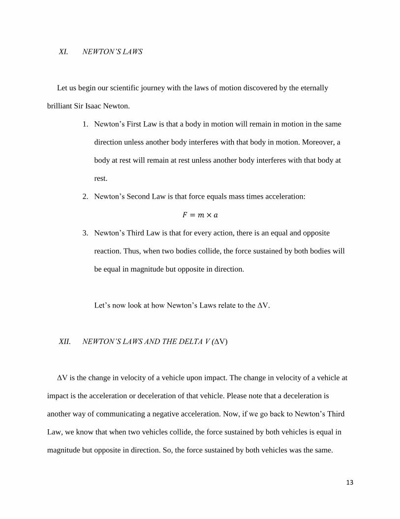
XI. NEWTON’S LAWS

Let us begin our scientific journey with the laws of motion discovered by the eternally

brilliant Sir Isaac Newton.

1. Newton’s First Law is that a body in motion will remain in motion in the same

direction unless another body interferes with that body in motion. Moreover, a

body at rest will remain at rest unless another body interferes with that body at

rest.

2. Newton’s Second Law is that force equals mass times acceleration:

3. Newton’s Third Law is that for every action, there is an equal and opposite

reaction. Thus, when two bodies collide, the force sustained by both bodies will

be equal in magnitude but opposite in direction.

Let’s now look at how Newton’s Laws relate to the ΔV.

XII. NEWTON’S LAWS AND THE DELTA V (ΔV)

ΔV is the change in velocity of a vehicle upon impact. The change in velocity of a vehicle at

impact is the acceleration or deceleration of that vehicle. Please note that a deceleration is

another way of communicating a negative acceleration. Now, if we go back to Newton’s Third

Law, we know that when two vehicles collide, the force sustained by both vehicles is equal in

magnitude but opposite in direction. So, the force sustained by both vehicles was the same.

14

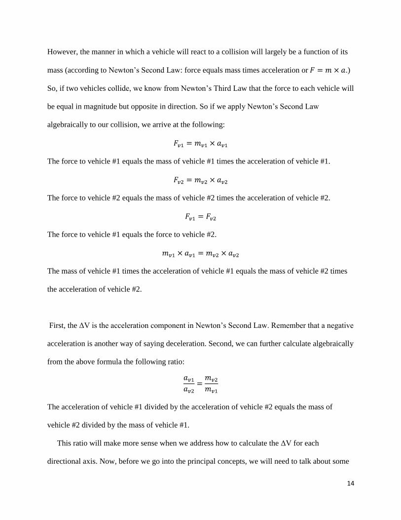
However, the manner in which a vehicle will react to a collision will largely be a function of its

mass (according to Newton’s Second Law: force equals mass times acceleration or .)

So, if two vehicles collide, we know from Newton’s Third Law that the force to each vehicle will

be equal in magnitude but opposite in direction. So if we apply Newton’s Second Law

algebraically to our collision, we arrive at the following:

The force to vehicle #1 equals the mass of vehicle #1 times the acceleration of vehicle #1.

The force to vehicle #2 equals the mass of vehicle #2 times the acceleration of vehicle #2.

The force to vehicle #1 equals the force to vehicle #2.

The mass of vehicle #1 times the acceleration of vehicle #1 equals the mass of vehicle #2 times

the acceleration of vehicle #2.

First, the ΔV is the acceleration component in Newton’s Second Law. Remember that a negative

acceleration is another way of saying deceleration. Second, we can further calculate algebraically

from the above formula the following ratio:

The acceleration of vehicle #1 divided by the acceleration of vehicle #2 equals the mass of

vehicle #2 divided by the mass of vehicle #1.

This ratio will make more sense when we address how to calculate the ΔV for each

directional axis. Now, before we go into the principal concepts, we will need to talk about some

15

elementary concepts in physics. Do not lose patience. Just keep reading. It will all make sense

after you have read this manuscript in its entirety.

XIII. ELEMENTARY PHYSICS

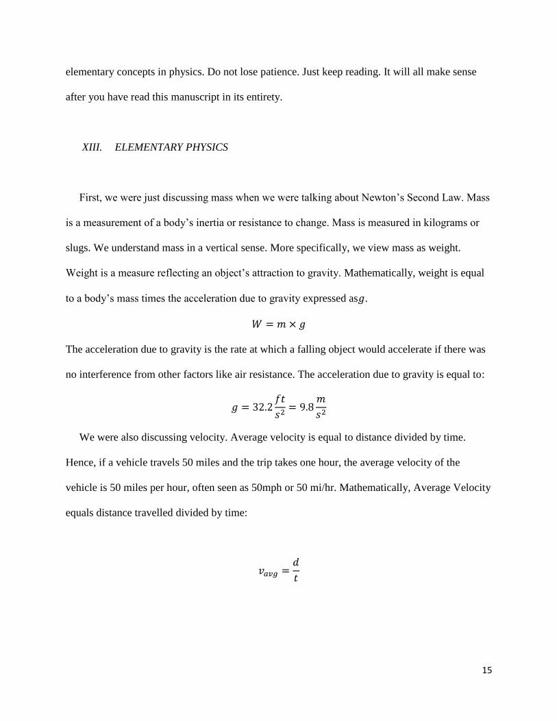
First, we were just discussing mass when we were talking about Newton’s Second Law. Mass

is a measurement of a body’s inertia or resistance to change. Mass is measured in kilograms or

slugs. We understand mass in a vertical sense. More specifically, we view mass as weight.

Weight is a measure reflecting an object’s attraction to gravity. Mathematically, weight is equal

to a body’s mass times the acceleration due to gravity expressed as .

The acceleration due to gravity is the rate at which a falling object would accelerate if there was

no interference from other factors like air resistance. The acceleration due to gravity is equal to:

We were also discussing velocity. Average velocity is equal to distance divided by time.

Hence, if a vehicle travels 50 miles and the trip takes one hour, the average velocity of the

vehicle is 50 miles per hour, often seen as 50mph or 50 mi/hr. Mathematically, Average Velocity

equals distance travelled divided by time:

16

The term velocity often gets confused with the term speed. Velocity is a vector quantity and

speed is a scalar quantity. A vector quantity has both magnitude and direction. A scalar quantity

has only magnitude.

In addition, we have been talking about acceleration. As previously mentioned deceleration is

a negative acceleration. So do not get confused when we just use the word acceleration to mean

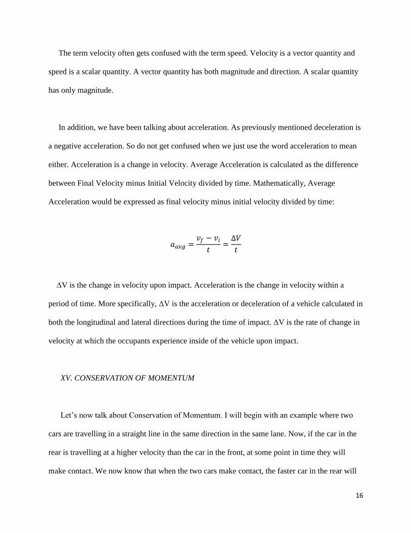
either. Acceleration is a change in velocity. Average Acceleration is calculated as the difference

between Final Velocity minus Initial Velocity divided by time. Mathematically, Average

Acceleration would be expressed as final velocity minus initial velocity divided by time:

ΔV is the change in velocity upon impact. Acceleration is the change in velocity within a

period of time. More specifically, ΔV is the acceleration or deceleration of a vehicle calculated in

both the longitudinal and lateral directions during the time of impact. ΔV is the rate of change in

velocity at which the occupants experience inside of the vehicle upon impact.

XV. CONSERVATION OF MOMENTUM

Let’s now talk about Conservation of Momentum. I will begin with an example where two

cars are travelling in a straight line in the same direction in the same lane. Now, if the car in the

rear is travelling at a higher velocity than the car in the front, at some point in time they will

make contact. We now know that when the two cars make contact, the faster car in the rear will

17

transfer energy to the slower car in the front. More specifically, the car in the rear will lose

energy and the car in the front will gain energy. The car in the rear will decelerate and the car in

the front will accelerate. However, notwithstanding the transfer of energy between the two cars,

according to the Law of Conservation of Momentum, as long as an outside force does not

interfere with the momentum of either of the two vehicles, the sum of the momentum of the two

vehicles before the collision, will equal the sum of the momentum of the two vehicles after the

collision.

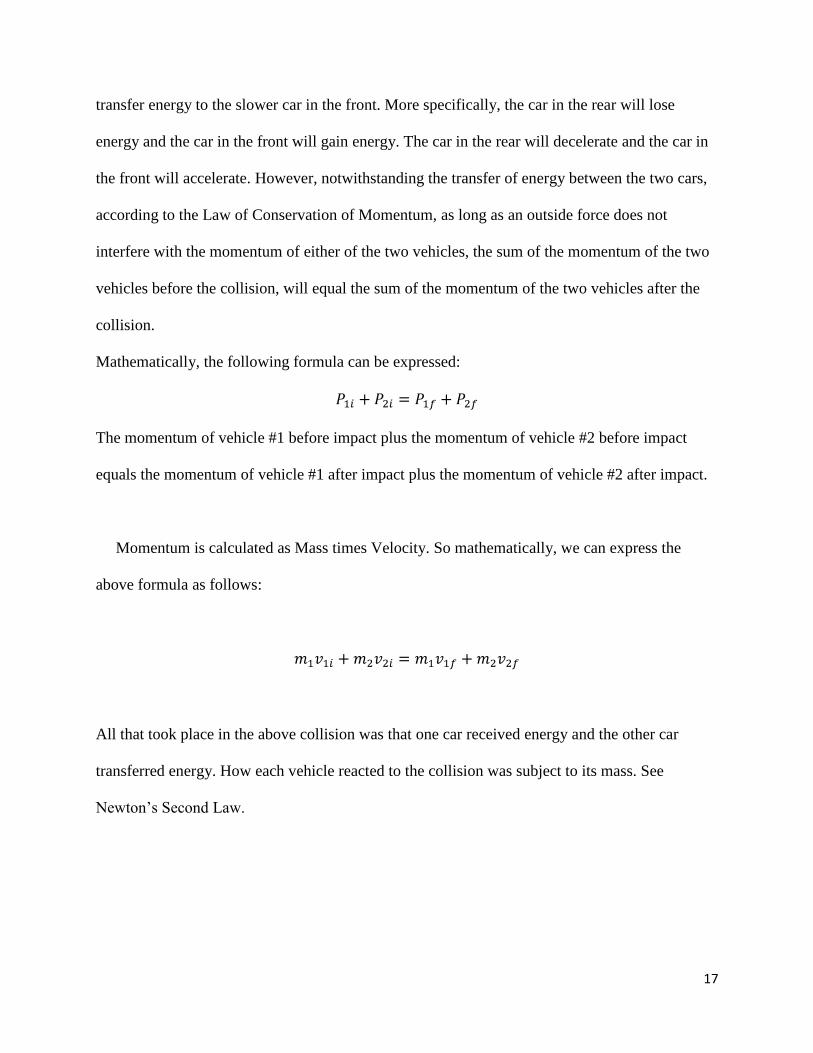
Mathematically, the following formula can be expressed:

The momentum of vehicle #1 before impact plus the momentum of vehicle #2 before impact

equals the momentum of vehicle #1 after impact plus the momentum of vehicle #2 after impact.

Momentum is calculated as Mass times Velocity. So mathematically, we can express the

above formula as follows:

All that took place in the above collision was that one car received energy and the other car

transferred energy. How each vehicle reacted to the collision was subject to its mass. See

Newton’s Second Law.

18

Conservation of Momentum must be preserved in both the longitudinal and lateral directions.

For example, if we have a perpendicular type of impact in which a car heading north sustains a

frontal impact into the passenger doors of a car heading east, both cars will be decelerated for

their respective longitudinal directions of travel. Moreover, the car heading north will be

accelerated east and the car heading east will be accelerated north. However, momentum will be

conserved for both the northern and eastern directions of travel.

If we would like to use the Law of Conservation of Momentum to support the calculations for

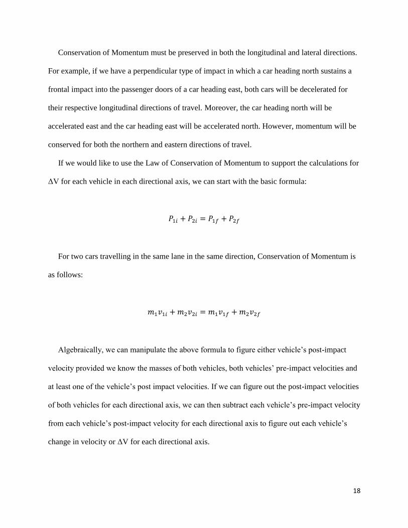
ΔV for each vehicle in each directional axis, we can start with the basic formula:

For two cars travelling in the same lane in the same direction, Conservation of Momentum is

as follows:

Algebraically, we can manipulate the above formula to figure either vehicle’s post-impact

velocity provided we know the masses of both vehicles, both vehicles’ pre-impact velocities and

at least one of the vehicle’s post impact velocities. If we can figure out the post-impact velocities

of both vehicles for each directional axis, we can then subtract each vehicle’s pre-impact velocity

from each vehicle’s post-impact velocity for each directional axis to figure out each vehicle’s

change in velocity or ΔV for each directional axis.

19

XVI. CLOSING SPEED

The Closing Speed is the net velocity of the two vehicles coming together on the same

directional axis. Remember that when calculating ΔV, we need to calculate a ΔV for both the

longitudinal directional axis and the lateral directional axis. So going back to our initial example

of the rear-end collision, let’s call the faster car in the rear the bullet and let’s call the slower car

in the front the target. The closing speed on the longitudinal directional axis is the pre-impact

velocity of the bullet or rear-vehicle minus the pre-impact velocity of the target or front vehicle.

For example, if the car in the rear is going 95 mph and the car in the front is going 90 mph, as

long as no external forces interfere, for our purposes of determining the ΔV, the accident is no

different than if the car in the rear was going 25 mph and the car in the front was going 20 mph.

More specifically, we are strictly concerned with the energy that transfers, which is linearly

related to the ΔV. So, if the car in the rear is going 95 mph and the car in the front is going 90

mph, the closing speed is 5 mph. The two cars are coming together in the longitudinal direction

at 5 mph. If the car in the rear is going 25 mph and the car in the front is going 20 mph, the

closing speed in the longitudinal direction is 5 mph.

Let’s talk about perpendicular collisions, which are a bit more complicated. Let’s begin with

an example. If a car, which is heading north sustains a frontal impact into the passenger side

doors of a car heading east; there are both longitudinal and lateral ΔV’s for both vehicles.

However, we can only calculate a closing speed for the northbound car that sustains a frontal

impact. The closing speed will be equal to the northbound car’s contact speed or speed at which

20

the northbound car made contact with the car going east. We will talk more about this, when I

address how to calculate the ΔV. For right now, let’s talk about contact speeds.

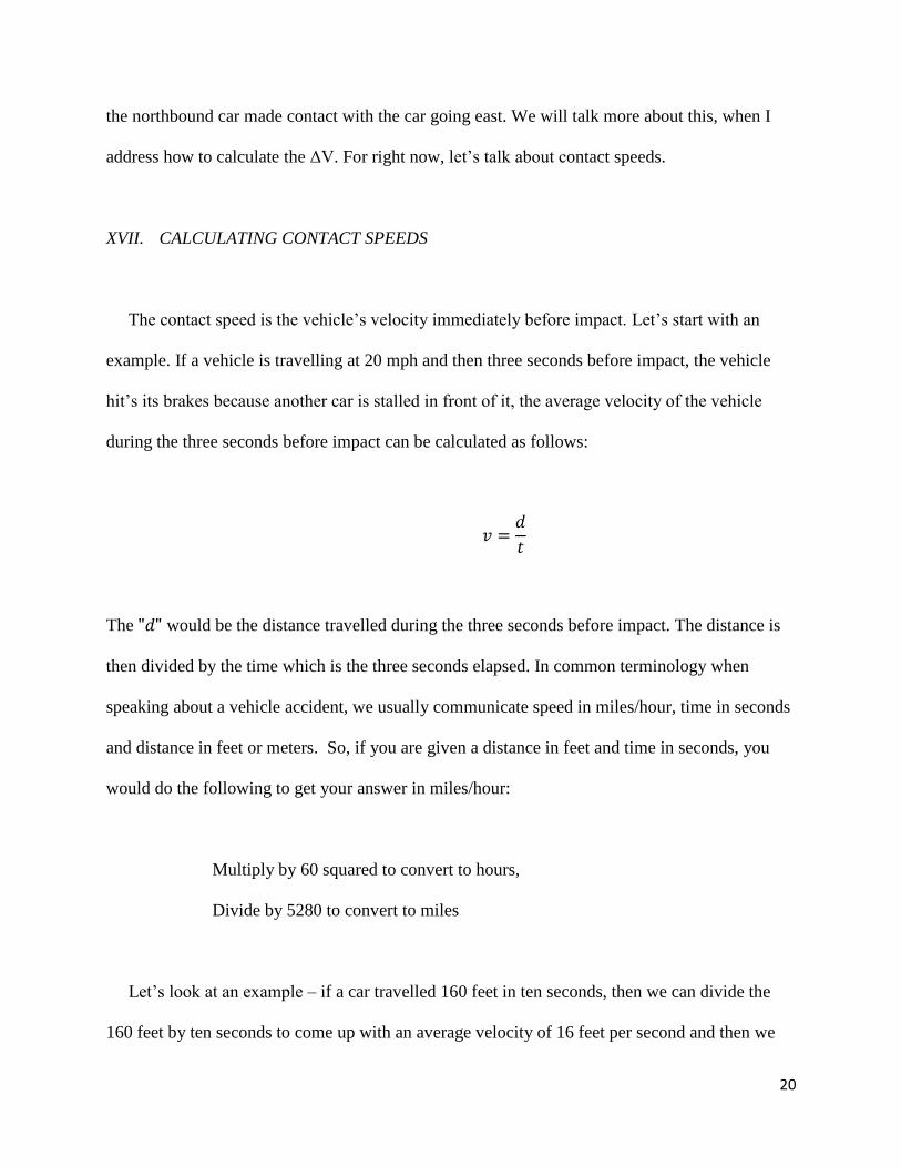
XVII. CALCULATING CONTACT SPEEDS

The contact speed is the vehicle’s velocity immediately before impact. Let’s start with an

example. If a vehicle is travelling at 20 mph and then three seconds before impact, the vehicle

hit’s its brakes because another car is stalled in front of it, the average velocity of the vehicle

during the three seconds before impact can be calculated as follows:

The would be the distance travelled during the three seconds before impact. The distance is

then divided by the time which is the three seconds elapsed. In common terminology when

speaking about a vehicle accident, we usually communicate speed in miles/hour, time in seconds

and distance in feet or meters. So, if you are given a distance in feet and time in seconds, you

would do the following to get your answer in miles/hour:

Multiply by 60 squared to convert to hours,

Divide by 5280 to convert to miles

Let’s look at an example – if a car travelled 160 feet in ten seconds, then we can divide the

160 feet by ten seconds to come up with an average velocity of 16 feet per second and then we

21

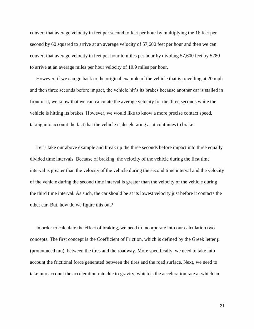
convert that average velocity in feet per second to feet per hour by multiplying the 16 feet per

second by 60 squared to arrive at an average velocity of 57,600 feet per hour and then we can

convert that average velocity in feet per hour to miles per hour by dividing 57,600 feet by 5280

to arrive at an average miles per hour velocity of 10.9 miles per hour.

However, if we can go back to the original example of the vehicle that is travelling at 20 mph

and then three seconds before impact, the vehicle hit’s its brakes because another car is stalled in

front of it, we know that we can calculate the average velocity for the three seconds while the

vehicle is hitting its brakes. However, we would like to know a more precise contact speed,

taking into account the fact that the vehicle is decelerating as it continues to brake.

Let’s take our above example and break up the three seconds before impact into three equally

divided time intervals. Because of braking, the velocity of the vehicle during the first time

interval is greater than the velocity of the vehicle during the second time interval and the velocity

of the vehicle during the second time interval is greater than the velocity of the vehicle during

the third time interval. As such, the car should be at its lowest velocity just before it contacts the

other car. But, how do we figure this out?

In order to calculate the effect of braking, we need to incorporate into our calculation two

concepts. The first concept is the Coefficient of Friction, which is defined by the Greek letter µ

(pronounced mu), between the tires and the roadway. More specifically, we need to take into

account the frictional force generated between the tires and the road surface. Next, we need to

take into account the acceleration rate due to gravity, which is the acceleration rate at which an

22

object would fall if no other factors like air resistance were present. Let us begin our analysis

with the formula to calculate contact speed when a vehicle is decelerating due to braking.

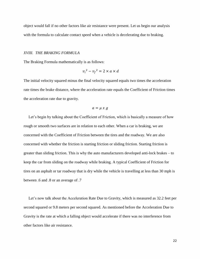
XVIII. THE BRAKING FORMULA

The Braking Formula mathematically is as follows:

The initial velocity squared minus the final velocity squared equals two times the acceleration

rate times the brake distance, where the acceleration rate equals the Coefficient of Friction times

the acceleration rate due to gravity.

Let’s begin by talking about the Coefficient of Friction, which is basically a measure of how

rough or smooth two surfaces are in relation to each other. When a car is braking, we are

concerned with the Coefficient of Friction between the tires and the roadway. We are also

concerned with whether the friction is starting friction or sliding friction. Starting friction is

greater than sliding friction. This is why the auto manufacturers developed anti-lock brakes – to

keep the car from sliding on the roadway while braking. A typical Coefficient of Friction for

tires on an asphalt or tar roadway that is dry while the vehicle is travelling at less than 30 mph is

between .6 and .8 or an average of .7

Let’s now talk about the Acceleration Rate Due to Gravity, which is measured as 32.2 feet per

second squared or 9.8 meters per second squared. As mentioned before the Acceleration Due to

Gravity is the rate at which a falling object would accelerate if there was no interference from

other factors like air resistance.

23

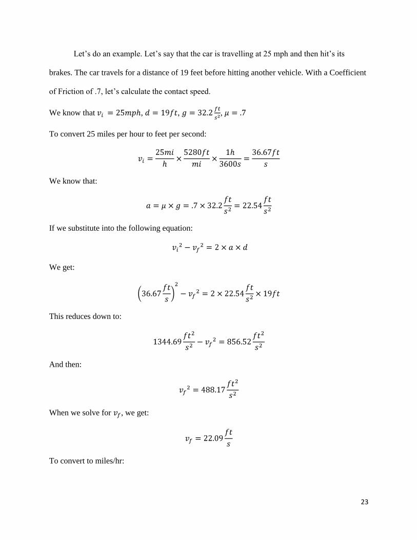
Let’s do an example. Let’s say that the car is travelling at 25 mph and then hit’s its

brakes. The car travels for a distance of 19 feet before hitting another vehicle. With a Coefficient

of Friction of .7, let’s calculate the contact speed.

We know that , , ,

To convert 25 miles per hour to feet per second:

We know that:

If we substitute into the following equation:

We get:

This reduces down to:

And then:

When we solve for , we get:

To convert to miles/hr:

24

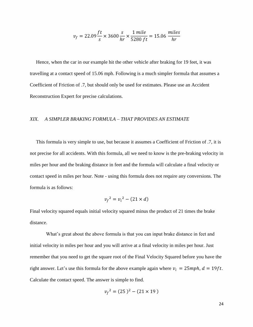
Hence, when the car in our example hit the other vehicle after braking for 19 feet, it was

travelling at a contact speed of 15.06 mph. Following is a much simpler formula that assumes a

Coefficient of Friction of .7, but should only be used for estimates. Please use an Accident

Reconstruction Expert for precise calculations.

XIX. A SIMPLER BRAKING FORMULA – THAT PROVIDES AN ESTIMATE

This formula is very simple to use, but because it assumes a Coefficient of Friction of .7, it is

not precise for all accidents. With this formula, all we need to know is the pre-braking velocity in

miles per hour and the braking distance in feet and the formula will calculate a final velocity or

contact speed in miles per hour. Note - using this formula does not require any conversions. The

formula is as follows:

Final velocity squared equals initial velocity squared minus the product of 21 times the brake

distance.

What’s great about the above formula is that you can input brake distance in feet and

initial velocity in miles per hour and you will arrive at a final velocity in miles per hour. Just

remember that you need to get the square root of the Final Velocity Squared before you have the

right answer. Let’s use this formula for the above example again where , .

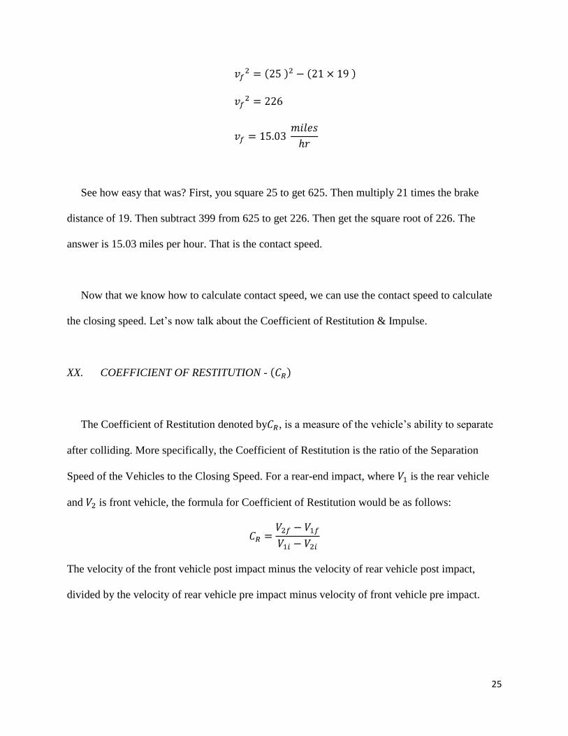
Calculate the contact speed. The answer is simple to find.

25

See how easy that was? First, you square 25 to get 625. Then multiply 21 times the brake

distance of 19. Then subtract 399 from 625 to get 226. Then get the square root of 226. The

answer is 15.03 miles per hour. That is the contact speed.

Now that we know how to calculate contact speed, we can use the contact speed to calculate

the closing speed. Let’s now talk about the Coefficient of Restitution & Impulse.

XX. COEFFICIENT OF RESTITUTION -

The Coefficient of Restitution denoted by , is a measure of the vehicle’s ability to separate

after colliding. More specifically, the Coefficient of Restitution is the ratio of the Separation

Speed of the Vehicles to the Closing Speed. For a rear-end impact, where is the rear vehicle

and is front vehicle, the formula for Coefficient of Restitution would be as follows:

The velocity of the front vehicle post impact minus the velocity of rear vehicle post impact,

divided by the velocity of rear vehicle pre impact minus velocity of front vehicle pre impact.

26

Now, let’s talk about elasticity. The elasticity of a collision is whether the cars bounce off

each other when colliding or stick together. Elasticity is part of the Coefficient of Restitution. In

a perfectly elastic collision, the two bodies collide and then bounce off of each other. There is no

deformation of the bodies. In a perfectly inelastic collision, upon colliding the two bodies stick

together and there is much deformation or crush to the bodies. A perfectly elastic collision,

where there is no deformation, would be a Coefficient of Restitution equal to the number one. A

perfectly inelastic collision, where there is much deformation and sticking together, the

Coefficient of Restitution would be equal to zero.

As you will see shortly when we examine the ΔV formula, the lower the Coefficient of

Restitution, the less effect it has on the ΔV. Remember that a Coefficient of Restitution of zero

represents lots of crush or sticking together. Whereas, a Coefficient of Restitution of one is

where the cars bounce off each other and there is minimal deformation.

Okay, we covered a lot of material. We have two final subjects to address on the topic of ΔV.

First, we will cover the mathematical calculation of the ΔV and then, we will address, Energy

Crush Analysis.

27

XXI. MATHEMATICAL FORMULA FOR DELTA V- (ΔV)

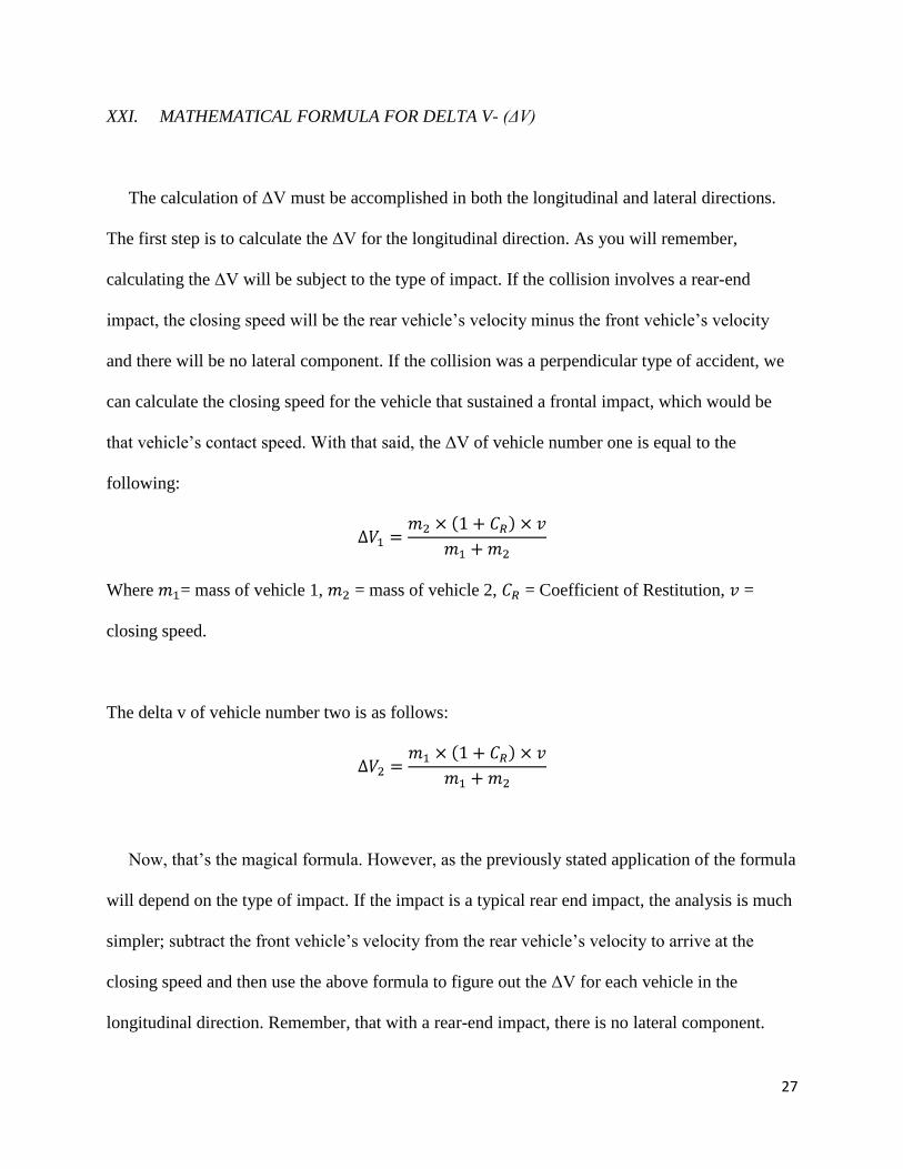
The calculation of ΔV must be accomplished in both the longitudinal and lateral directions.

The first step is to calculate the ΔV for the longitudinal direction. As you will remember,

calculating the ΔV will be subject to the type of impact. If the collision involves a rear-end

impact, the closing speed will be the rear vehicle’s velocity minus the front vehicle’s velocity

and there will be no lateral component. If the collision was a perpendicular type of accident, we

can calculate the closing speed for the vehicle that sustained a frontal impact, which would be

that vehicle’s contact speed. With that said, the ΔV of vehicle number one is equal to the

following:

Where = mass of vehicle 1, = mass of vehicle 2, = Coefficient of Restitution, =

closing speed.

The delta v of vehicle number two is as follows:

Now, that’s the magical formula. However, as the previously stated application of the formula

will depend on the type of impact. If the impact is a typical rear end impact, the analysis is much

simpler; subtract the front vehicle’s velocity from the rear vehicle’s velocity to arrive at the

closing speed and then use the above formula to figure out the ΔV for each vehicle in the

longitudinal direction. Remember, that with a rear-end impact, there is no lateral component.

28

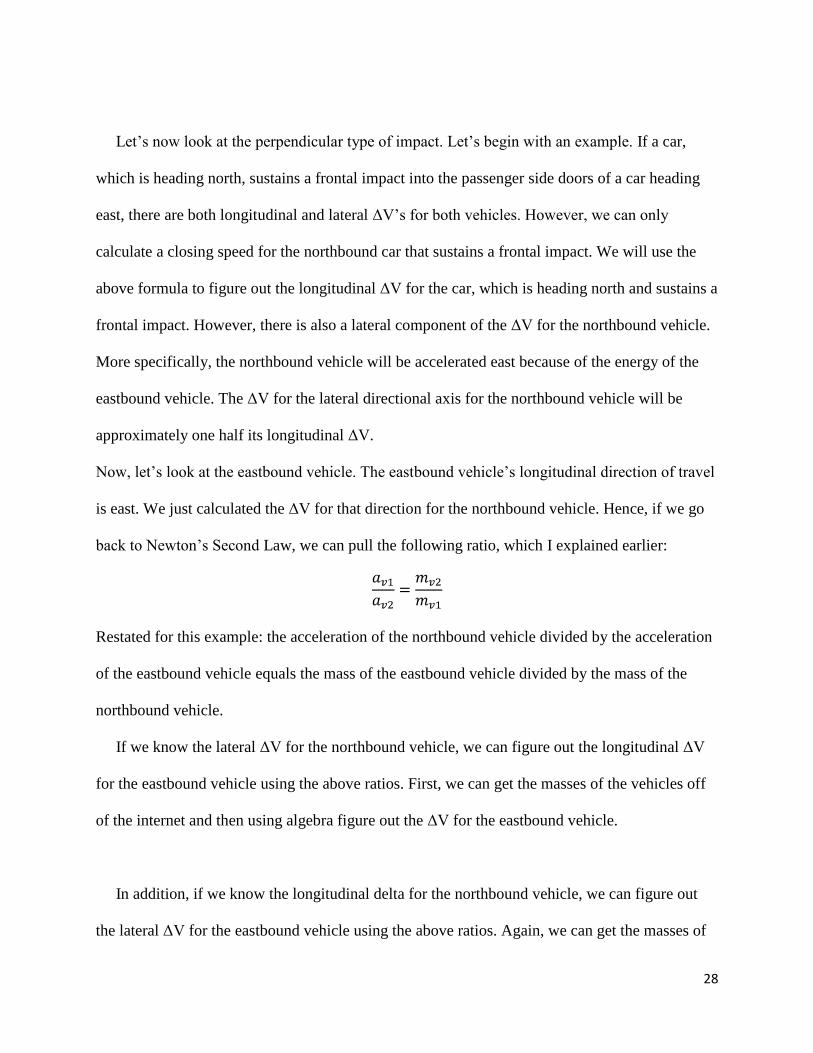
Let’s now look at the perpendicular type of impact. Let’s begin with an example. If a car,

which is heading north, sustains a frontal impact into the passenger side doors of a car heading

east, there are both longitudinal and lateral ΔV’s for both vehicles. However, we can only

calculate a closing speed for the northbound car that sustains a frontal impact. We will use the

above formula to figure out the longitudinal ΔV for the car, which is heading north and sustains a

frontal impact. However, there is also a lateral component of the ΔV for the northbound vehicle.

More specifically, the northbound vehicle will be accelerated east because of the energy of the

eastbound vehicle. The ΔV for the lateral directional axis for the northbound vehicle will be

approximately one half its longitudinal ΔV.

Now, let’s look at the eastbound vehicle. The eastbound vehicle’s longitudinal direction of travel

is east. We just calculated the ΔV for that direction for the northbound vehicle. Hence, if we go

back to Newton’s Second Law, we can pull the following ratio, which I explained earlier:

Restated for this example: the acceleration of the northbound vehicle divided by the acceleration

of the eastbound vehicle equals the mass of the eastbound vehicle divided by the mass of the

northbound vehicle.

If we know the lateral ΔV for the northbound vehicle, we can figure out the longitudinal ΔV

for the eastbound vehicle using the above ratios. First, we can get the masses of the vehicles off

of the internet and then using algebra figure out the ΔV for the eastbound vehicle.

In addition, if we know the longitudinal delta for the northbound vehicle, we can figure out

the lateral ΔV for the eastbound vehicle using the above ratios. Again, we can get the masses of

29

the vehicles off of the internet and then using algebra figure out the ΔV for the eastbound

vehicle.

What’s important is that we understand that the ΔV must be calculated for each directional

axis. The northbound car’s longitudinal directional acceleration is the eastbound car’s lateral

directional acceleration. The northbound vehicle’s lateral acceleration is the eastbound vehicle’s

longitudinal directional acceleration. However, we have to figure all of this out starting with the

closing speed of the northbound vehicle which is equal to its contact speed. In this scenario, we

can only find the closing speed of the vehicle which sustained a frontal impact. We then use that

closing speed to figure out the longitudinal ΔV for the northbound vehicle using the

ΔV formula and then we take one half of the result as the lateral ΔV. We then use the above

ratios to calculate the ΔV for the eastbound vehicle using the northbound vehicle’s ΔV’s, but we

must be careful to use the appropriate directional axis because momentum must be conserved in

each direction.

Now, let’s talk about Energy Crush Analysis, which is also used to figure out ΔV’s.

XXII. ENERGY CRUSH ANALYSIS

A Biomechanical Engineer can calculate the amount of energy transferred or lost in a

collision by analyzing the crush to a vehicle. Only one vehicle is needed because the force

sustained by both vehicles in a collision is the same. The force is equal in magnitude but opposite

in direction for both vehicles (See Newton’s Third Law). Let’s start with an example. If you have

two identical cars built to specification in the same manner with the same materials, we can

30

agree that if we hit one of the vehicles with a certain amount of force in a certain manner and

location, the dent or deformation that will result will be almost identical to the dent or

deformation that will result when we hit the other vehicle with the same amount of force in the

same manner and location. So if we can accept the premise that a vehicle’s deformation will

reflect the amount of energy absorbed or lost in a collision, then can we also accept the premise

that an identically built vehicle will deform in the same manner as its twin if both vehicles

sustain the same amount of force in the same location in the same manner.

Now, if we can accept the above, why can’t we use crash test studies to see how other

vehicles of the same make and model deformed under crash test scenarios in which all of the

data was measured and recorded? These tests serve as a point of measurement by which we can

determine the ΔV for the accident vehicle by comparing the amount of energy absorbed in the

present collision against the amount of energy absorbed by the crash test vehicle. At the very

least, the crash test vehicle should serve as an upper bound. We can further support the analysis

with mathematical calculation taking into account everything that we have been talking about up

until know.

That concludes our discussion of the ΔV. Let’s now talk about Biomechanics and the human

anatomy and physiology.

31

BIOMECHANICS AND THE HUMAN ANATOMY & PHYSIOLOGY

I. ANATOMY OF THE HUMAN SPINE

The spine is made of a number of bony structures called vertebrae that stack one on top of the

other. Each vertebral body has basically a hole through it called the vertebral foramen that is

essentially the pathway for the spinal cord. The spinal cord is the main conduit of the nervous

system almost like a wiring harness, and at different points along the spine, bundles of nerves

called nerve roots branch off to the far reaches of the human body. There are cushions between

each vertebra called intervertebral discs that isolate the vertebral bone structures which are

flexible structures, almost like a jelly doughnut. These essentially serve as shock absorbers for

the vertebra and maintain flexibility of the spinal column. These intervertebral discs have a

strong fibrous but flexible outer covering called that annulus fibrosis with an inner fluid called

the nucleus pulposus which has the consistency of toothpaste. The spine consists of three major

regions: cervical (C1-C7), thoracic (T1-T12) and lumbar (L1-L5), along with the sacrum and

coccyx.

II. INJURY CAUSING MECHANISMS OF THE HUMAN SPINE

The most common injuries referenced in low impact auto accidents are intervertebral disc

bulges and/or herniations. Damage or injury to intervertebral discs occurs when a situation

creates both a mechanism for injury and enough force to exceed the strength capacity of the disc

material. The mechanism for intervertebral disc herniations is hyper flexion or hyperextension

32

and a combination of lateral bending with an application of a sudden compressive load.

However, the most common disc injury is typically the result from chronic degeneration

produced by repetitive loading.

III. ANATOMY OF THE HUMAN KNEE

The knee is an anatomically dense area where muscles, tendons, ligaments and bone come

together. Generally, it is the joint where the femur (upper leg bone) and tibia (lower leg bone)

come together. The primary articulation of the knee joint involves motion of the femoral

condyles which are the two curved portions of the bottom portion of the femur, against the top

portion of the tibia. Contact between the femur and the tibia occurs in two places: medial and

lateral. The lateral and medial menisci are pieces of fibrocartilage that are attached to the top of

the tibia called the tibial plateau. These crescent shaped structures of varied thickness and

contour function as shock absorbers between the femur and the tibia.

The knee includes a redundant set of muscles and ligaments that control and stabilize the

joint. The ligaments we will address are the ACL (anterior cruciate ligament), PCL (posterior

cruciate ligament), MCL (medial collateral ligament) and LCL (lateral collateral ligament).

These ligaments restrain any forward, backward or side motion of femur across the tibia.

IV. INJURY CAUSING MECHANISMS OF THE HUMAN KNEE

Injuries to the knee joint happen when an incident occurs where enough force is applied in a

33

way that exceeds the tolerance or strength capacity of the effected tissue. The typical mechanism

for meniscal injury is twisting of the knee when the knee is weight bearing and flexed. More

specifically; an acute meniscus tear can only occur if the knee experiences substantial

compressive loading combined with simultaneous sliding of the femur relative to the tibial

plateau. For example: when a football player is impacted at the knee while cutting. Although

meniscal tears can be caused by traumatic injury, injuries are very widely attributed to

degeneration due to wear and tear.

Tears in the ACL and PCL can be injured in the same manner as the meniscus with a “plant

and twist”. The PCL can also be injured by falling on a bent knee or a strong frontal blow to the

lower part of a bent leg. The ACL can also be injured by a hyperextension of the lower leg.

MCL and LCL tears are most often caused by an impact to the side of the knee. Ligament tears

are typically trauma related.

V. ANATOMY OF THE HUMAN SHOULDER

The shoulder is a ball-and-socket type joint, where the head of the humerus (upper arm

bone) represents the ball portion of the joint and the glenoid cavity represents the socket. Since

this articulation is between the humerus and the glenoid, the primary ball-and socket joint of

the shoulder is also referred to as the glenohumeral joint. The glenoid labrum is a

fibrocartilaginous ring that lines the glenoid cavity of the shoulder joint.

The rotator cuff tendon consists of the conjoined tendons of the four rotator cuff muscles of

34

the shoulder: supraspinatus, infraspinatus, subscapularis, and teres minor. These tendons pass

under the coracoacromial arch, consisting of the acromion, acromioclavicular joint,

coracoacromialligament, and coracoid, and fuse to form a cuff surrounding the humeral head

before they insert into the humerus.

VI. INJURY CAUSING MECHANISMS OF THE SHOULDER

Due to the design of the shoulder, all movements of the shoulder, especially overhead

movements, compress the rotator cuff tendon repeatedly against the coracoacromial arch. The

repeated compression over time may result in degenerative pathology defined as a rotator cuff

tears. Many will attribute the onset of symptoms to a specific traumatic event, but a rotator cuff

tear is of chronic origin related to multiple factors such as overuse and aging. The rotator cuff is

commonly injured during repetitive use of the upper limb above the horizontal plane in activities

such as throwing, racket sports and swimming.

Impingement syndrome is the term used for the irritation of the tendons and bursa from

repeated contact with the undersurface of the acromion. This also is associated with repetitive

trauma caused by occupational or athletic endeavors and/or degenerative bony growth projecting

outward from the surface of the bone.

Injuries to the glenoid labrum can occur during a sudden impact that forces the head of the

humerus into the glenoid cavity. For example: falling on an outstretched arm.

35

ABOUT THE AUTHORS:

Sean O'Loughlin, Esq., President - a former Trial Attorney and Accountant; a graduate of

Brooklyn Law School and Baruch College; an executive who was directly responsible for

creating & developing American Transit Insurance Company's Special Operations Department

and Biomechanical Program; a co-author of the "Biomechanical Manual for Automobile

Litigation" and was a featured speaker for the New York State Bar Association's seminar titled

"Establishing the Biomechanical Defense."

John T. Montalbano, Vice President & Chief Operating Officer - an Engineer with over 15

years of engineering experience, including biomechanics, neuroscience, medical devices &

ultrasound; a former managing engineer in American Transit Insurance Company's

Biomechanical Program; a graduate of Polytechnic University; a co-author of the

"Biomechanical Manual for Automobile Litigation" and was a featured speaker for the New York

State Bar Association's seminar titled "Establishing the Biomechanical Defense."