the analysis of multigrid algorithms for - american ... of computation volume 51, number 184 october...
TRANSCRIPT
MATHEMATICS OF COMPUTATIONVOLUME 51, NUMBER 184OCTOBER 1988, PAGES 389-414
The Analysis of Multigrid Algorithms for
Nonsymmetric and Indefinite Elliptic Problems*
By James H. Bramble, Joseph E. Pasciak, and Jinchao Xu
Abstract. We prove some new estimates for the convergence of multigrid algorithms
applied to nonsymmetric and indefinite elliptic boundary value problems. We provide
results for the so-called 'symmetric' multigrid schemes. We show that for the variable
2^-cycle and the ^-cycle schemes, multigrid algorithms with any amount of smoothing
on the finest grid converge at a rate that is independent of the number of levels or
unknowns, provided that the initial grid is sufficiently fine. We show that the 2^-cycle
algorithm also converges (under appropriate assumptions on the coarsest grid) but at
a rate which may deteriorate as the number of levels increases. This deterioration for
the ^-cycle may occur even in the case of full elliptic regularity. Finally, the results of
numerical experiments are given which illustrate the convergence behavior suggested by
the theory.
1. Introduction. In recent years, multigrid methods have been used extensively
as tools for obtaining the solution of the discrete systems which arise in the nu-
merical approximation of partial differential equations (cf. [6], [8]). In conjunction,
there has been intensive research aimed at attaining a more thorough theoretical
understanding of the multigrid technique [l]-[5], [8], [13]-[18], [21]. In this paper,
we shall provide some new iterative convergence estimates for multigrid algorithms
applied to nonsymmetric and indefinite problems.
The theory for the analysis of multigrid methods applied to symmetric positive
definite problems is most completely developed [2], [4], [5], [13], [15], [21]. Generally,
these results assume a 'regularity and approximation' hypothesis which involves a
parameter 0 < a < 1. The results in these papers guarantee convergence rates for
multigrid 2^-cycle, the variable î^-cycle (cf. [5]) and the 5^-cycle algorithms for
various a. In particular, [5], [15] give iterative convergence results for the symmetric
problem which are valid for any amount of smoothing and any a.
The theory for multigrid methods applied to nonsymmetric and indefinite prob-
lems is not so completely developed. Two types of algorithms are the so-called
'symmetric' and 'nonsymmetric' multigrid schemes. The nonsymmetric scheme
uses a relaxation procedure based on the original equations whereas the symmetric
Received November 9, 1987.
1980 Mathematics Subject Classification (1985 Revision). Primary 65N30; Secondary 65F10.
"This manuscript has been authored under contract number DE-AC02-76CH00016 with the
U.S. Department of Energy. Accordingly, the U.S. Government retains a non-exclusive, royalty-
free license to publish or reproduce the published form of this contribution, or allow others to
do so, for U.S. Government purposes. This work was also supported in part under the National
Science Foundation Grant No. DMS84-05352 and under the Air Force Office of Scientific Research,
Contract No. ISSA86-0026 and by the U.S. Army Research Office through the Mathematical
Science Institute, Cornell University.
©1988 American Mathematical Society0025-5718/88 $1.00 + $.25 per page
389
License or copyright restrictions may apply to redistribution; see http://www.ams.org/journal-terms-of-use
390 JAMES H. BRAMBLE, JOSEPH E. PASCIAK, AND JINCHAO XU
scheme uses a relaxation based on the symmetric positive definite system associ-
ated with the normal equations. Some results only hold under rather restrictive
assumptions involving the relation between the number of smoothings m and the
size of the coarsest grid hj. For example, Bank [1] gives 3^-cycle results for both
schemes and for arbitrary a which, however, require first that m be sufficiently
large, and secondly that hj be sufficiently small (depending on m). Mandel [14]
gives results for the nonsymmetric ^-cycle scheme and the 2^-cycle scheme (as-
suming full regularity a = 1) which are valid for any m if hj is chosen sufficiently
small (depending on m).
In this paper, we shall prove some new iterative convergence estimates for the
symmetric multigrid scheme applied to nonsymmetric and indefinite problems. We
give results for the ^-cycle, variable 2^-cycle and 3^-cycle algorithms for any
amount of smoothing under the assumption of a > 3/4. Our theorems for the
variable 5^-cycle and ^"-cycle algorithms require that hj be sufficiently small (in-
dependent of the amount of smoothing) and guarantee an iterative convergence
rate which is uniformly independent of the number of levels and the mesh size on
the finest grid. The assumption that hj is sufficiently small is not very restrictive
since such an assumption must be made for solvability on the coarsest grid. The
results for the ^"-cycle algorithm are somewhat weaker. We show that the 2^-cycle
converges if hj is small enough (depending on the number of levels and a), at a
rate which deteriorates as more and more levels are used. Even in the case a = 1,
the 5^-cycle convergence estimates deteriorate like 1 — c/ln(/z_1).
We derive our iterative convergence estimates for multigrid algorithms in an
abstract setting. The use of this abstract approach more clearly identifies the
relevant hypotheses.
The outline of the remainder of the paper is as follows. In Section 2 we describe
the abstract framework to be used in the paper. The assumptions used in our
analysis and some preliminary definitions are also given there. Section 3 shows
how this framework can be applied in the case of nonsymmetric and indefinite
uniformly elliptic second-order boundary value problems. Section 4 defines the
multigrid operator and provides a basic recurrence relation used in our subsequent
analysis. The convergence estimates given in this paper are based on three technical
lemmas. In Section 5 we prove our multigrid theorems, assuming the technical
lemmas. Section 6 provides the proof of the lemmas and represents the core of
our analysis. Finally, the results of numerical experiments illustrating the earlier
derived theory are given in Section 7.
Throughout this paper, c and C, with or without subscript will denote a generic
positive constant which may take on different values in different places. These
constants will always be independent of the mesh parameters.
2. Abstract Framework and Assumptions. In this section, we first give
an abstract framework for our nonsymmetric multigrid application. This abstract
presentation more clearly identifies the relevant hypotheses used in the iterative
convergence analysis to be developed. We then list the assumptions required for
the multigrid analysis presented in later sections. To keep the paper from becoming
too abstract, we show how a model application to a second-order problem fits into
this framework in the next section.
License or copyright restrictions may apply to redistribution; see http://www.ams.org/journal-terms-of-use
MULTIGRID ALGORITHMS FOR ELLIPTIC PROBLEMS 391
We start with a Hubert scale (cf. [11]) of spaces {/P} for 7 E [0,2]. The norm
on H"1 will be denoted by || - ||j/-r. We assume that Hs c H* whenever t < s. The
largest space (i.e., 7 = 0) will be denoted H with norm || • \\n and inner product
(■,■). The space H1 is assumed to be compactly contained in H6 whenever 7 > 6.
Let JÍ be a closed subspace of H1. The spaces Hs for -1 < s < 0 are defined by
duality and with norm given by
cbeJf \m\H-'
Assume that we are given a nested sequence of 'approximation' subspaces
J?i C J?i c • • • C Jfj c Jt.
In addition, let A (-, ■) be a positive definite symmetric quadratic form on Jü x J[
satisfying
(2.1) c\\v\\2Hi < À (v, v) < C\\v\\2H, for all v E J?
and D (-, •) be a quadratic form on Jf x^#. We shall be interested in approximating
the solution of
(2.2) A (u, <p) = Â (u, </>) + D (u, <t>) = (f, 4>) for all <j> E Jt,
for a given function f E H. We shall assume that (2.2) is uniquely solvable for any
fEH.We will be interested in applying multigrid procedures to develop a rapidly
converging iterative algorithm for the solution of the Galerkin approximation of
(2.2) in the subspace Jij. Specifically, we seek the function U E J?j which satisfies
(2.3) A(U,X) = (f,x) forcûlxEJTj.
Our multigrid algorithms will require the use of discrete inner products (•, -)fc on
J^k x Jtk for fc = 1,... , J. The corresponding norm will be denoted || • ||fc. In the
algorithms, these inner products are used instead of (•, •) to avoid the inversion of
Gram matrices. This means that the problem of computing W E ^ satisfying
(2.4) {W,O)k = F(0) forallöe^ffc
for a given linear functional F should be simple.
We next list the assumptions required for our multigrid analysis.
(A.l): The first assumption involves elliptic regularity for the forms A(-,-) and
A (■, •). We assume that solutions u of (2.2) and the corresponding equation
 (u, B) = (f, 9) for aüOeJt
satisfy
(2.5) ||«||k»+. < cil/H*-,
for some a E (3/4,1] independent of /.
(A.2): We assume first that D satisfies
(2.6) |Z?(w,w)|<C|H|ffi||«;||H for al\v, wE J?.
License or copyright restrictions may apply to redistribution; see http://www.ams.org/journal-terms-of-use
392 JAMES H. BRAMBLE, JOSEPH E. PASCIAK, AND JINCHAO XU
It is an immediate consequence of (2.6) that the operator D : ^# i—> H defined by
(Dv, 9) = D (v, 6) for all 9 E H
is well defined and satisfies
(2.7) \\Dv\\H <C\\v\\Ht.
We further assume that D maps Hl+a into Ha, i.e.,
(2.8) \\Dv\\h° < C\\v\\Hi+a.
Let D* : H h» H~l be defined by
(D*w,4>) = (w,D4>).
We assume that D* is a bounded operator from H1 into i7_1/2~£ for any posi-
tive 6.
(A.3): We require approximation properties for the subspaces {^k}- These are
given in terms of a parameter hk which satisfies
CKk < hk < CKk
for constants c, C and k < 1 independent of fc. We assume that for v in Hs and
s E [1,1 + a], there exists \ £ -^k such that
II« - Xll/i + hk\\v - xlltfi < Chsk\\v\\Hs.
(A.4): We require that the inverse inequality,
\\W\\HB < Chl-0\\W\\Hi for all W EJ?k
holds for all ß > 7 with ß, 7 6 [0,1 + a].
(A.5): We require first that the discrete inner product (-,-)* be equivalent to
(■,■) on^fc, i.e.,
(2-9) c||x||ff<||x!U<C||x||H.
In addition, we assume that the discrete inner products accurately approximate the
inner product on H in the sense that
(2.10) \{ib,x)-{rb,x)k\<Chk\\ib\\H1\\x\\k for all V,X € ^ffc.
We next introduce some discrete operators which play a fundamental role both
in the analysis and the algorithms to be considered in this paper:
(0.1): The operator Ak : J^k •-> -^k is defined by
(AkW,9)k = A(W,9) forallöe^ffc.
(0.2): The operator Pk : -^ >->■ -^k is defined by
(2.11) A(Pkw,9) = A(w,9) for all 9 E Jtk.
(0.3): The operator Ak : ̂ #¿ •-► Jfk is defined by
(ÂkW,6)k=Â(W,9) for t\\\ 9 E J?k-
License or copyright restrictions may apply to redistribution; see http://www.ams.org/journal-terms-of-use
MULTIGRID ALGORITHMS FOR ELLIPTIC PROBLEMS 393
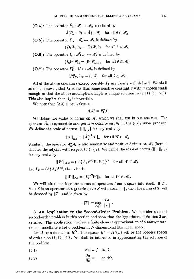
(0.4): The operator Pk : *# >-► Jtk is defined by
Â(Pkw,9) = Â(w,9) for all 9 eJtk.
(0.5): The operator Dk : ̂ k *-* -^k is defined by
(DkW, 9)k = D (W, 9) for all 9 E Jtk.
(0.6): The operator Ik : ̂ k+i •->• Jtk is defined by
(IkW, 9)k = (W, 9)k+x for all 9 E Jfk.
(0.7): The operator P% : H v-^, Jfk\s defined by
(Pj¡v, 9)k = (v, 9) for all 9 E Jtk.
All of the above operators except possibly Pk are clearly well defined. We shall
assume, however, that hk is less than some positive constant u with u chosen small
enough so that the above assumptions imply a unique solution to (2.11) (cf. [20]).
This also implies that Ak is invertible.
We note that (2.3) is equivalent to
AkU = Pfc0/.
We define two scales of norms on Jfk which we shall use in our analysis. The
operator Ak is symmetric and positive definite on Jfk in the (•, )fc inner product.
We define the scale of norms {||-||fc s} for any real s by
W\\kta = \\ÂfW\\k for a\\WE^k-
Similarly, the operator A*kAk is also symmetric and positive definite on JKk (here, *
denotes the adjoint with respect to (•, -)k). We define the scale of norms {||| • |||fc,s}
for any real s by
\\\W\\\kia = ((A*kAk)s/2W, W)l/2 for all W E JTk.
Let Lk = (A*kAk)1/2; then clearly
Pik« = \\LfW\\k for all W E J[k.
We will often consider the norms of operators from a space into itself. If T :
S i—» S is an operator on a generic space S with norm || • ||, then the norm of T will
be denoted by ||T|| and is given by
mi=SuPra0€S 11011
3. An Application to the Second-Order Problem. We consider a model
second-order problem in this section and show that the hypotheses of Section 2 are
satisfied. This application involves a finite element approximation of a nonsymmet-
ric and indefinite elliptic problem in A^-dimensional Euclidean space.
Let Í2 be a domain in RN. The spaces Hs — HS(Q) will be the Sobolev spaces
of order s on fi [12], [19]. We shall be interested in approximating the solution of
the problem
(3.1) &u = f in ÎÎ,
3ii(3.2) — = 0 on dû,
ov
License or copyright restrictions may apply to redistribution; see http://www.ams.org/journal-terms-of-use
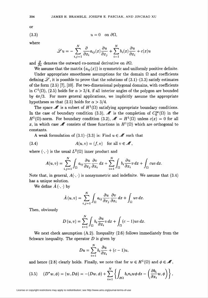
394 JAMES H. BRAMBLE, JOSEPH E. PASCIAK, AND JINCHAO XU
or
(3.3) u = o on an,
whereN a a N a
3u = - ) — atJ (x-h ) bi(x)-r— +c(x)u
1,3 = 1 J t=l
and #- denotes the outward co-normal derivative on dU.ov
We assume that the matrix {atj(x)} is symmetric and uniformly positive definite.
Under appropriate smoothness assumptions for the domain O and coefficients
defining J?', it is possible to prove that the solutions of (3.1)-(3.3) satisfy estimates
of the form (2.5) [7], [10]. For two-dimensional polygonal domains, with coefficients
in C1(Q), (2.5) holds for a > 3/4, if all interior angles of the polygon are bounded
by 47t/3. For more general applications, we implicitly assume the appropriate
hypotheses so that (2.5) holds for a > 3/4.
The space ^# is a subset of i/^fi) satisfying appropriate boundary conditions.
In the case of boundary condition (3.3), JÍ is the completion of Co°(fi) in the
iY1(n)-norm. For boundary condition (3.2), JÍ = H1^) unless c(x) = 0 for all
x, in which case ./# consists of those functions in H1 (fi) which are orthogonal to
constants.
A weak formulation of (3.1)-(3.3) is: Find uEJf such that
(3.4) A(u,v) = (f,v) for alined,
where (•, •) is the usual L2(Q) inner product and
A(u,v) = > / an-—-—dx + > / bi~—vdx+ / cuvdx.^Jn dxjdxi ^Jn dxi Jn
t,J = l z=l
Note that, in general, A(-, ■) is nonsymmetric and indefinite. We assume that (3.4)
has a unique solution.
We define Â(-,-) by
2 , n v~» Í du dv , fA(u,v) = > / an-—-—ax + / uvax.
■ • , Jn dx, dxi jn1,3 = 1
Then, obviously
N
D (u, v) = y / bi ——v dx + / (c — l)uv dx.f^Jn oxi j0
We next check assumption (A.2). Inequality (2.6) follows immediately from the
Schwarz inequality. The operator D is given by
£)li = ^6t-^- + (c-l)ti,t=i x%
and hence (2.8) clearly holds. Finally, we note that for w E Hl(Vl) and <f> E Jt',
(3.5) (D*w,4>) = (w,D<t>) = -(Dw,<p) + J2Íf biniW(t>ds-(^w,A\,
License or copyright restrictions may apply to redistribution; see http://www.ams.org/journal-terms-of-use
MULTIGRID ALGORITHMS FOR ELLIPTIC PROBLEMS 395
where n¿ is the component of the outward normal in the ith direction. We assume
that bi is in C1(fi) and that c is in L°°(fi). The boundary term in (3.5) vanishes
in the case of boundary conditions (3.3) and hence D* : H1(Q) i-> L2(dU) in this
case. In the case of boundary conditions (3.2), by a well-known trace inequality,
N
birtiwtfids < C ||w|l/p/2+£(n) il^lljîi/2+^n)
N .
i=i Jan
from which it follows that D* : H^Q) ■-» i/"1/2"^). Thus (A.2) holds for either
application.
We next consider the finite element approximation subspaces. For simplicity,
we shall only describe a piecewise linear application in two dimensions. The appli-
cation to higher-dimensional problems and more general approximation subspaces
is straightforward. We write Q — \Jrj-, where ri = {r/} is a collection of trian-
gles with mutually disjoint interiors. We assume that these triangles are of quasi-
uniform size hi. This means that there are positive constants c and C such that the
diameter of every triangle is bounded by Chi and each triangle contains a circle of
radius chi. We define a sequence of triangulations by induction. Assume that the
triangulation rk-i — {V,fc_1} has been defined. The triangles of rk are formed by
connecting the midpoints of the edges of the triangles in Tk-i- Thus, each triangle
in Tk-i gives rise to four triangles in Tk-
The approximation subspace J?k consists of functions which are continuous and
piecewise linear with respect to the triangulation Tk- In the case of Dirichlet bound-
ary conditions, we additionally require that the functions in Tk vanish on <9fi. In the
case of boundary conditions (3.2) and c(x) = 0, we also require that the functions in
Tk have zero mean value. For these spaces, hk = 2~k+1hi and classical techniques
in the theory of finite elements imply that (A.3) and (A.4) hold.
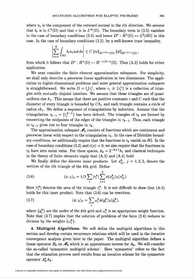
We finally define the discrete inner products. Let xkL, j = 1,2,3, denote the
vertices of the ith triangle of the fcth grid. Define
3
(3-6) (4>,X)k = l/3Çtfl5>(4)x(*&)-t j=i
Here |r*| denotes the area of the triangle rk. It is not difficult to show that (A.5)
holds for this inner product. Note that (3.6) can be rewritten
(3.7) (*,x)* = £«M»?)x(0?).i
where {yk} are the nodes of the fcth grid and uk is an appropriate weight function.
Note that (3.7) implies that the solution of problems of the form (2.4) reduces to
division by the weights {u>k}.
4. Multigrid Algorithms. We will define the multigrid algorithms in this
section and develop certain recurrence relations which will be used in the iterative
convergence analysis given later in the paper. The multigrid algorithm defines a
linear operator Bk on J?k which is an approximate inverse for Ak- We will consider
the so-called 'symmetric multigrid scheme'. Here 'symmetric' refers to the fact
that the relaxation process used results from an iterative scheme for the symmetric
operator A*kAk-
License or copyright restrictions may apply to redistribution; see http://www.ams.org/journal-terms-of-use
396 JAMES H. BRAMBLE, JOSEPH E. PASCIAK, AND JINCHAO XU
We define the operator Bk : J?k *->■ -^k by induction on fc. As we shall see in later
sections, for stability, the coarsest grid in the multigrid process must not be too
coarse. To this end, we shall define our algorithms starting from the intermediate
grid level j, 1 < j < J. In this algorithm, we assume that the operator Bj equals
AJ1, although some results still hold when Bj is defined differently (see Remark
5.2).
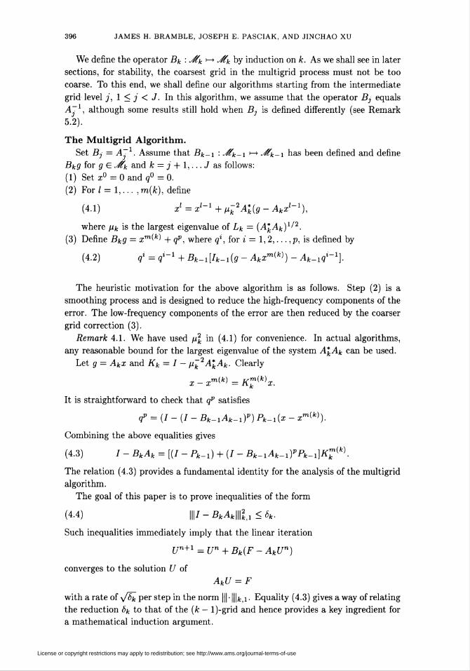
The Multigrid Algorithm.
Set Bj = A~l. Assume that Bk-i : ̂ k-i ^ -^fe-i has been defined and define
Bkg for g E ^k and k — j + I,.. .J as follows:
(1) Set z° = 0 and q° = 0.
(2) For 1 = 1,... ,m(k), define
(4.1) xl = xl-l+p-k2Al(g-Akx1-1),
where pk is the largest eigenvalue of Lk = (A*kAk)1/2.
(3) Define Bkg = zm(fc) + qp, where ql, for i = 1,2,... ,p, is defined by
(4.2) «f = q*-1 + Bfc-il/fc-ite - Akxm^) - Afc-H*"1].
The heuristic motivation for the above algorithm is as follows. Step (2) is a
smoothing process and is designed to reduce the high-frequency components of the
error. The low-frequency components of the error are then reduced by the coarser
grid correction (3).
Remark 4.1. We have used pk in (4.1) for convenience. In actual algorithms,
any reasonable bound for the largest eigenvalue of the system A*kAk can be used.
Let g = Akx and Kk = I — pk2A*kAk. Clearly
x-x^)=Kkn{k)x.
It is straightforward to check that qp satisfies
qp = (/-(/ - Bk-iAk-i)p) Pk-i(x - xm^).
Combining the above equalities gives
(4.3) / - BkAk = [(I - Pk-i) + (I- Bk-iAk-ifPk-i\K{k).
The relation (4.3) provides a fundamental identity for the analysis of the multigrid
algorithm.
The goal of this paper is to prove inequalities of the form
(4-4) \\\I-BkAk\\\li<6k.
Such inequalities immediately imply that the linear iteration
jjn+i = un + Bk(F-AkUn)
converges to the solution U of
AkU = F
with a rate of y/i\ per step in the norm ||| • \^k,i ■ Equality (4.3) gives a way of relating
the reduction 6k to that of the (fc - l)-grid and hence provides a key ingredient for
a mathematical induction argument.
License or copyright restrictions may apply to redistribution; see http://www.ams.org/journal-terms-of-use
MULTIGRID ALGORITHMS FOR ELLIPTIC PROBLEMS 397
5. The Convergence Theorems and their Proofs. We give our convergence
results for multigrid algorithms in this section. We first give results for the variable
2^-cycle. Next, we consider the 2^-cycle with constant m(k) = m. Finally, we
consider the 3F-cycle algorithms. The proofs of these theorems depend on three
lemmas. These lemmas are central to the analysis of the paper and will be proved
in the next section. In this section, we prove our multigrid theorems, assuming the
lemmas.
We start by stating the lemmas. The first lemma gives a so-called 'regularity
and approximation' estimate for the projection operator TV
LEMMA 5.1. If hj is sufficiently small, there exists a positive constant C not
depending on fc such that
||(7 - Pk-i)v\\\ < C(pkl \\Lkv\\2k)a(Lkv, v)l~a for all v E Jtk.
The next two lemmas represent an essential part of the analysis of this paper.
Their proof uses the Dunford-Taylor integral formula for operators and is given in
the next section.
LEMMA 5.2. If hj is sufficiently small, there exists a positive constant C not
depending on k such that for all v E ^#fe, x £ -$k-i,
(5.1) (Lk(I - Pk-i)v,x)k <Chak-1/2~£\\\(I - Pk-i)v\\\k,i\\\x\\\k,i
holds for any positive e.
LEMMA 5.3. If hj is sufficiently small, there exists a positive constant C not
depending on k such that for all x € ^fc-i,
1111x1111,1 - lllxlllUil < Chka~\i + MfcDiiixMî,!.We can now state and prove the convergence theorem for the variable 2^-cycle
algorithm.
THEOREM 1. Let p = 1 and assume that m(k) satisfies
(5.2) ß0m(k) < m(k - 1) < ßim(k)
where ßo and ßi are constants greater than one and independent of k for k =
j + 2,... ,J. Let 7 be positive and less than min (a — 1/2,4a — 3). Then there exist
positive constants M and v not depending on k such that when hj < v, (4.4) holds
with
(5-3) 6k = M + m(k)«/2
for k = j + 1,... , J.
Proof. We will prove the theorem by induction. For the purpose of this proof,
let m(j) = ßotn(j + 1) (note that m(j) does not appear in the definition of the
multigrid process). Clearly, (4.4) holds for fc = j with Ok given by (5.3). Let
fc E {j + 1,... , J} and assume that (4.4) holds for fc - 1 with 6k-i given by (5.3).
It follows from the recursive relation (4.3) that
|||(7 - BkAk)v\\\ltl = |||(7 - Pk-i)v\\\2kA + |||(7 - Bk-iAk-i)Pk-iv\\\li
+ 2(Lk(I - Pk-i)i, (I - Bk-iAk-i)Pk~ii)k,
License or copyright restrictions may apply to redistribution; see http://www.ams.org/journal-terms-of-use
398 JAMES H. BRAMBLE, JOSEPH E. PASCIAK, AND JINCHAO XU
where v — Kk 'v. Applying Lemma 5.2 gives
|||(/ -iMfcHIlL
< (1 + Chak-1/2~£) (111(7 - Pk-i)v\\\li + |||(7 - Bk_iAk^)Pk-ii\\\li).
Using Lemma 5.3 and the induction hypothesis, we deduce that
|||(7 - Bk-iAk_i)Pk_iv\\\li < (1 + Chl)\\\(I - Bk-iAk-i)Pk-iv\\\2k-hi
<6k-i(l + Chl)\\\Pk-iv\\\Uhi
<6k^i(l + Ch1)\\\Pk-iv\\\li
holds for any fixed 7 less than 4a - 3. We remind the reader that here and through-
out the paper, C denotes a generic positive constant which may take on different
values from line to line. It follows from Lemma 5.2 that
\\\v\\\li = \\\Pk-iv\\\li + |||(7 - Pk-i)v\\\li + 2(Lk(I - Pk-i)v, Pk-iv)k
> (1 - Chak-1/2-e)(\\\Pk-ii\\\l,i + III (/ - Pk-i)v\\\l,i)
and thus for v sufficiently small
ipv-iiiii^ < (1+c/*r 1/2-£)iNi2fc,i - mu - Pk-i)v\tk,i-
Requiring, in addition, that 7 < a —1/2 and combining the above inequalities gives
|||(7 - BkAk)v\\\li < (1 + Ch]) {(1 - 4-i)|||(7 - Pk-i)v\\\li + 6k-i\\\v\\\li} -
By Lemma 5.1, the Schwarz inequality, and a generalized arithmetic geometric
mean inequality,
|||(7 - Pk-i)v\\\li < C {pk\L2i,v)k)a (Lki,v)k~a
<C(pk2(Llv,v)k)a/2(Lkv,v)k-a/2
<c{mpk2(Llv,^k + nka,{*~a)(LkvMk}
holds for any positive constant r)k- Using the definition of Kk and the fact that its
eigenvalues are in the interval [0,1) gives
p-k2(L\v,v)k = (Lk(I - Kk)K[k)v,K^v)k
2m(fc)-l
<(2m(fc))-x Y. (Lk(I - Kk)Klkv,v)k
1=0
= (2m(k))-\Lk(I - K2km{k))v,v)k.
Combining the above inequalities gives
|||(J -BkAk)v\\\ltl
(5.4) < (1 + Cihl)lco(l - ek-i)nkm(k)-\Lk(I - K2km(k))v, v)k
+ [Co(l - 6k-i)Vkan2~a)+6k-i](LkK2kmWv,v)ky
Setting C2 = Co(l + Ci), we see that the theorem will follow if we can choose
rjk, hj and M such that
(5.5) C2(l-8k.i)rlkm(k)-l<èk
License or copyright restrictions may apply to redistribution; see http://www.ams.org/journal-terms-of-use
MULTIGRID ALGORITHMS FOR ELLIPTIC PROBLEMS 399
and
(5.6) C2(l - 6k-i)r)ka/i2~a)+Cih]6k-i <6k- 6k-i.
We choose rjk by
(5.7) C2(l - ¿fc-i^mtfc)-1 = Sk-i,
from which (5.5) immediately follows. Solving for rjk in (5.7) and using this result
in (5.6) implies that it is sufficient to choose M and hj so that
(5.8) C3(l - 6k-i)2/{2-a)m(k)-a^2-^ + Cih]b2k'}2x-a) < (6k - 6k-i)6^~a).
Let 2S(k) = M + m(k)a/2 and ßk = m(fc - l)/m(fc) E [/?o,/?i]; then
<^\ 1 S (ßkm(k))a'2
A direct computation using (5.9) and the identity 6k = M/2>(k) shows that (5.8)
is equivalent to
(5.10) C3ßak/{2-a)M-^2~^ + Cih]M < M™(gj*/2 (ßak12 - 1).
Note that if M > 1 then
r_M«/2 iVQ< Mm(k)a>2 a/2 nC4 = (A> - !)/2 * M + m(jb)a/a (^ -1)'
hence it suffices to have
Q;M-Q/(2-o) + d/ijAf < d,
where C5 = C3/V . Thus, taking M > 1 large enough so that
<75M-Q/(2-Q) < C4/2
and
hj<v< C\h(2CiM)-lli
completes the proof of the theorem.
We next prove a theorem for the standard ^-cycle algorithm.
THEOREM 2. Consider the W-cycle algorithm (p = 1) with m(k) = m for
all fc. Let 7 be positive and less than min (a — 1/2,4a — 3). Then there exist
positive constants M, c, and v not depending on k such that when hj <
min(i/,c(j - l)"2/^)), (4.4) holds with
Mfc(2~a>/a
1 > k ~ (Mfc(2-Q)/Q+m«/2)
for k = j + l,... ,J.
Remark 5.1. The theorem suggests that the 2^-cycle may be less robust than the
variable 5^-cycle. Note that the convergence estimate for the 2^-cycle algorithm
deteriorates as fc becomes larger, even in the case a = 1. Furthermore, the theorem
suggests that for stability, the coarsest grid must become finer as the number of
grid levels increases.
License or copyright restrictions may apply to redistribution; see http://www.ams.org/journal-terms-of-use
400 JAMES H. BRAMBLE, JOSEPH E. PASCIAK, AND JINCHAO XU
Proof. The proof of this theorem is essentially contained in the proof of Theorem
1 and the proof of Theorem 1 of [5]. Indeed, (5.4) is valid with m(k) = m and hence
it suffices to choose r¡k, M, hj, and c so that (5.5) and (5.6) are satisfied. We choose
r)k by (5.7) and reduce (5.5)-(5.6) to (5.8). Making similar algebraic manipulations
(compare with (5.10)), we see it suffices to choose the parameters so that
C3M-Q/(2-a) +dh](k - 1)2/Q
<^w[^-a)/a-(k-i){2-a)/a)(k-i),
where 2>(k) = Mk^2-a^a+ma/2. Noting that fc > 2and(2-a)/a > 0, elementary
arguments imply
k(2-a)/a < C^k(2-a)/a _ (fc _ ^(a-oj/a] (fc _ -,)
Thus, it suffices to prove
MmQ/2fc(2-a'/a
We set
C3M-a/(a-a) + Cih]M(k - l)2'a < C6-
f-, ,->\(2_a)/a
and define A7 by
Then
C3M-a/(2_a) = Co/2.
r M-a/(2-a) < C6 M CeMnf^k^^CzM <___<_-__-.
We then set
c =C6M
2Ci(l + M),
from which it follows that hj < c(j - 1)_2/(tq) implies
Ca M Cr MmQ/2fc(2~a'/aCiK\M(k - 1)2/Q < ^-^T7 < ^ *,-.3 v ; - 2 1 + M - 2 3(k)
Combining the above inequalities proves the theorem.
The last theorem which we shall prove is for the 2F-cycle algorithm.
THEOREM 3. Consider the W-cycle algorithm (p = 2) with m(k) = m for all
fc. Let 7 be positive and less than min (a - 1/2,4a - 3). Then there exist positive
constants M and v such that when hj < v, (4.4) holds with
(5.12) 6k = 6 = (l + m/M)-a/2
for fc = j + 1,... , J.
Proof. The proof of this theorem is essentially contained in the proof of Theorem
1 and the proof of Theorem 3 of [5]. Since the term involving (7 - 73fc_i.4fc_i)
appears squared in (4.3), following the proof of Theorem 1, we see that (5.4) holds
License or copyright restrictions may apply to redistribution; see http://www.ams.org/journal-terms-of-use
MULTIGRID ALGORITHMS FOR ELLIPTIC PROBLEMS 401
with 6k-i replaced by ó2. We see that the theorem will follow if we can choose
Vk = *?! v and M such that
(5.13) C2(l-ö2)r/m-1 <6
and
(5.14) C2(l - ¿2)iTa/(2-Q) + Cih]S2 <6-62.
We choose r\ so that (5.13) holds with equality. Solving for r¡ and using this
result in (5.14) implies that it is sufficient to choose M and v so that
(5.15) C3(l - ¿2)2/(2-a)m-a/(2-a) + ^ ft7¿(4-a)/(2-a) < (1 _ ¿)¿2/(2-a)_
It is elementary to see that
(5.16) 2-V<-»<(1-i,-«/(-<.)(g)'""î-)(îl7)
for <S given by (5.12). Define M by
MQ/(2-a)2-2/(2-a) _ 2(o
2/(2-a)
ThenC3(l - ¿2)2/(2-Ci)m-a/(2-a) < 1(1 _ ¿)(c2/(2-a^
¿à
Choosing
(5.17) hj<v<
implies
(l-^lh
2Ci6
CiA75(4-a)/(2-a) < * (, _ ¿)(c2/(2-a)_J 2
This completes the proof of the theorem.
Remark 5.2. The multigrid process described in Section 4 requires that the prob-
lem on the coarsest grid be solved exactly, i.e., Bj = AJ1. It is possible to relax this
restriction and still apply the results of this paper. We consider, for example, the
variable J^-cycle multigrid algorithm. From the proof of Theorem 1 it is immediate
that the theorem will still hold as long as Bj satisfies
(5.18) W-BjAjMliKôj,
where
M(5.19) 6j =-To-.
M + /£/2m(i + l)«/2
One obvious choice for an iterative definition of B3 is B3g = x™1 where z for I =
1,... ,mj is given by (4.1) with fc = j. Here nij is some integer to be specified. An
iterative definition of B3 has the advantage that no additional coding is necessary
(in contrast to the use of Bj = AJ1, where direct solvers for nonsymmetric and
indefinite problems must be introduced into the code). There are two additional
factors involved in the use of an iterative process for Bj. First, one would like to
avoid the coarsest grids so that h3 < u is satisfied. Secondly, the computational
work on the coarsest grid should not increase the asymptotic work of the algorithm.
License or copyright restrictions may apply to redistribution; see http://www.ams.org/journal-terms-of-use
402 JAMES H. BRAMBLE, JOSEPH E. PASCIAK, AND JINCHAO XU
We consider the application described in Section 3. We should like the multigrid
algorithm to achieve a reduction 6j which is independent of hj , with computational
effort bounded by a constant times the number of grid points in the finest grid. Let
7V(fc) denote the number of degrees of freedom in the fcth grid level. We assume
N(k)/N(k — 1) > Co > ßi, and hence the amount of work on the grids 1,... , J
will be bounded by O (TV (J)) [3], [6]. It is not difficult to see that for Bj defined as
above,
W-BjAMh <(l-cfc$)m'.
On the other hand, if we take /?o = /?i = 2,
M + 2°/2m(j + l)"/2 * <W'Ai)a/a.
Consequently, to satisfy (5.18)—(5.19), we need only take
(5.20) rnj = 0(hj1h-3).
The work constraint is then h'j1^5 < ch~2. Thus setting hj = hj and defining
m.j by (5.20) gives rise to a multigrid algorithm which yields a uniform reduction in-
dependent of hj, with an operation count bounded by a constant times the number
of degrees of freedom on the finest grid.
6. The Proof of Lemmas 5.1, 5.2 and 5.3. This section will provide the
proofs of Lemmas 5.1-5.3. Before proceeding, let us state two propositions and two
preliminary lemmas.
PROPOSITION 6.1. There are positive constants c and C not depending on
v E ^ such that
\\v\\2m <C{A(v,v) + c\\v\\2H}.
PROPOSITION 6.2. For vE H1+a and 0 < 6 < a,
(6.1) ||(7-Pfc)t;||ffi-{ <Chi\\(I-Pk)v\\m.
If hj is sufficiently small, then Pk is well defined and
(6.2) \\(I - Pk)v\\H> <C inf \\v-x\\m,
for all v E Jf.
Proposition 6.1 follows immediately from (2.6). (6.1) follows from a standard
duality argument and (6.2) can be proved by using the techniques given in [20].
We next introduce the preliminary lemmas. The first lemma was essentially
proved in [1].
LEMMA 6.1. Let 0 < s < 1. There exist positive constants ci, c2 and c3 such
that
llxllJis < CiWxIlks ^ c2 llxllfc.s ^ c3||xI|ks for all x E JTk-
In addition, there are constants c and C satisfying
c\\\x\\\k,2 < ||xllfc,2 < G|llxlHfc,2 for all X e JTk.
License or copyright restrictions may apply to redistribution; see http://www.ams.org/journal-terms-of-use
MULTIGRID ALGORITHMS FOR ELLIPTIC PROBLEMS 403
LEMMA 6.2. There exists a positive constant C which does not depend upon
v E H1 such that
(6.3) \\(I-P°)v\\H<Chk\\v\\Hi,
(6.4) II**v||H. < C\\v\\Hs for allO<s<l.
Proof. Let kv denote the 77 projection of v into J?k- Using (A.3), (A.4) and
standard techniques of finite element analysis gives
IIHI/r <c|H|äi,\\(I-T)v\\H<Chk\\v\\Hl.
Forxe^fc,by(2.10),
((P% - tt)v, x)k = (irv, x) - ('tv, x)k < Chk\\irv\\Hi HxlU,
hence
\\(P%-*)v\\k<Chk\\irv\\Hi.
Estimate (6.3) follows from the triangle inequality.
For (6.4), by interpolation, it suffices to verify the cases s = 0 and s = I. The
case for s = 0 follows immediately from the definition of Pk and (2.9). For s = I,
the argument is standard and proceeds as follows:
||P^||Hi<||(P°-7rH|H1+|MI/ii
<Ch^\\(PS-ir)v\\k + C\\v\\H, <C|M|j,..
This completes the proof of the lemma.
We can now prove Lemma 5.1.
Proof of Lemma 5.1. Following the argument in [5], we can easily show (using
our assumptions and definitions) that
||(7 - tV-HI2 < C(h2k\\Âkv\\2)aÂ(v,v)1-" for all v E Jfk.
We note that (A.4) and Lemma 6.1 imply that h\ < Cp^1. The lemma now follows
from (6.2) and Lemma 6.1.
The proofs of Lemmas 5.2 and 5.3 require some technical perturbation estimates.
We consider the term on the left-hand side of (5.1). Let Gk = Lk — Ak\ then since
(Ak(I-Pk-i)v,x)k = 0,
we have
(Lk(I - Pk-i)v,x)k = (Gk(I - Pk-i)v,x)k = ((7 - Pk-i)v,Glx)k
<||(/-ft-i)ti|UI|GixlU.
Thus, we must estimate G*k = Lfc — Ak — Dk.
In light of (6.5), we see that it would be useful to estimate the difference Lk -Ak-
Note that Lk is defined as the positive square root of the discrete operator L\ =
A*kAk- An alternative expression for Lk is given by the Dunford-Taylor integral
representation (cf. [9]):
(6.6) Lk = (2«)-1 Í zll2mz(L\) dz,
T
License or copyright restrictions may apply to redistribution; see http://www.ams.org/journal-terms-of-use
404 JAMES H. BRAMBLE, JOSEPH E. PASCIAK, AND JINCHAO XU
where ¿^¿(L2.) = (z — Lk)_1 and T is a simple closed curve in the right half (com-
plex) plane which encloses the spectrum of L\. Let /c1,/c2 > 0 be such that the
eigenvalues of L\ and A\ are in the interval [2/ci, k2]. In this paper, we will take T
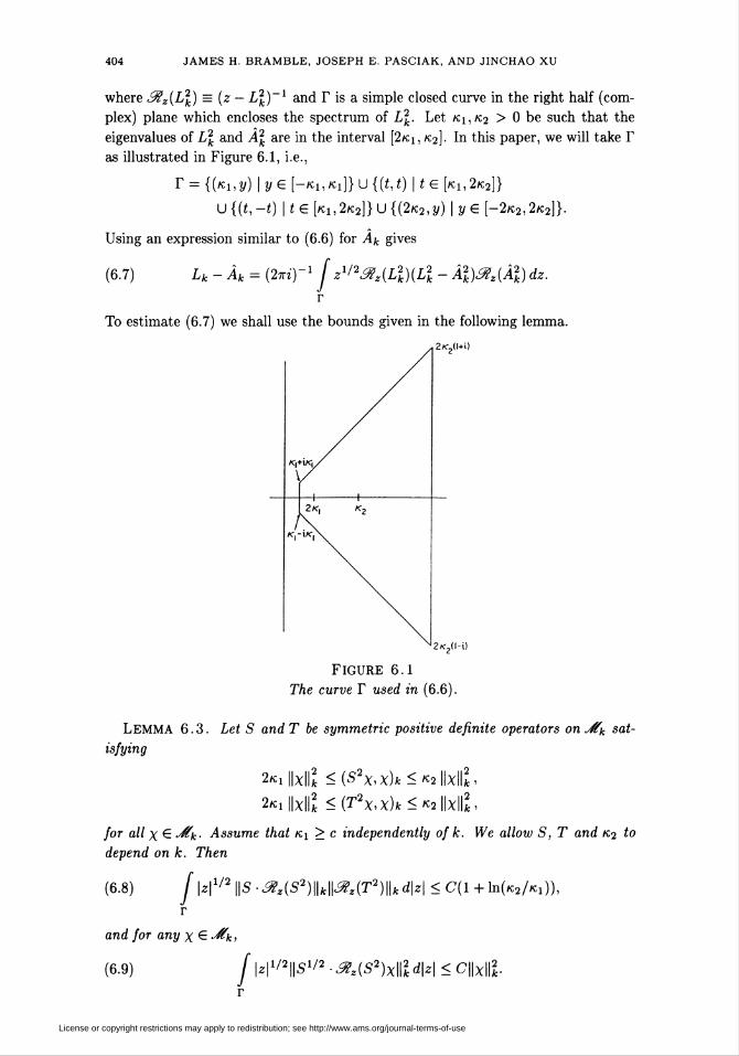
as illustrated in Figure 6.1, i.e.,
r = {(«i,y) \ye[-Ki,Ki]}u{(t,t) |íg[ki,2k2]}
U {(t, -t)\tE [k, , 2k2}} U {(2«2,y) | y E {-2k2,2k2}}.
Using an expression similar to (6.6) for Ak gives
(6.7) Lk - Ak = (2m)-1 jz^2^z(L2)(L2 - Â2)<%Z(Â\) dz.
T
To estimate (6.7) we shall use the bounds given in the following lemma.
Figure 6.1
The curve T used in (6.6).
LEMMA 6.3. Let S andT be symmetric positive definite operators on J?k sat-
isfying
2/ci||x||fc < (S2X,x)k < K2||xllfc,
2*i||x|fi <(T2X,x)k<rZ2\\x\\2k,
for all x S JUk- Assume that ni > c independently of fc. We allow S, T and k2 to
depend on fc. Then
(6.8) j \z\x/2 \\S ■ ̂(S2)\\k\\^(T2)\\k d\z\ < C(l + \n(K2/Ki)),
r
and for any x £ -^k,
(6-9) J\znsV2-^z(S2)x\\2kd\z\<C\\x\\l
License or copyright restrictions may apply to redistribution; see http://www.ams.org/journal-terms-of-use
MULTIGRID ALGORITHMS FOR ELLIPTIC PROBLEMS 405
and
Proof. By symmetry, it suffices to derive the above bounds for the curve r+ =
r,ur2ur3, where ri s {(/ci,y) | ye [O,/^]}, T2 = {(t,t) \ t E [rCi,2/c2]} and
T3 = {(2/c2,y) | y E [0,2/c2]}. By expansion in terms of eigenvectors, it is easy to
see that
(6.10) \\Sß&,{S2)\\k < max Xß\X2-z\-\ 0 = 0,1/2,1.
A similar inequality obviously holds for T.
Let
^i(l) = j\z\ll2\\S-^z(S2)\\k\\âêz(T2)\\kd\z\
i
W1) = f\z\í"\\s1'2-a,{3*Mld\z\.i
Then by (6.10) and elementary estimates,
&¡{Ti) <c Í\z\1/2rtx3/2d\z\ < C,
r,
^¡(T2)<CÍ \z\-1d\z\<C\n(2K2/Ki),
^ï(r3)<C H -^^dy<C.Jo k2 + y
This verifies (6.8). Similar arguments give
Wi) S C If \z\'* K-,'12 d\z\ ] llxlli < C
j,(r,)sc(r q5?*)wssoM
i2Ifc '
To bound 5*2(Y2), we expand in terms of the eigenvectors of 5. Let {A¿, 0¿} denote
the eigenvalue-eigenvector pairs for the operator 5. Without loss of generality, we
may assume that {0¿} form an orthornormal basis for JKj. Clearly, 2/ci < X2 < k2
holds for each i. Decomposing
X = ^2 Ci9ii
gives
\\S1/2-^(S2)x\\2k = Z\yTT7ü-
Integrating term by term yields
(6.11) mi) = p^fJ_^Ç_dt.Elementary manipulations show that the integrals in (6.11) are bounded uniformly
in ki,k2, and A¿. Hence ^(r2) < C \\x\\k- This completes the proof of the lemma.
We now state and prove a lemma for estimating Lk — Ak-
License or copyright restrictions may apply to redistribution; see http://www.ams.org/journal-terms-of-use
406 JAMES H. BRAMBLE, JOSEPH E. PASCIAK, AND JINCHAO XU
LEMMA 6.4. Let hj be sufficiently small. Then there exists a constant C such
that for all x £ ^k,
\\LkX - ÂkxWm < Chak~l(l + | In A*|)||4fexl|fc
and
\\LkX-ÀkX\\k<Chak-l\\x\\m-
Proof. By Lemma 6.1,
\\LkX- ÂkxWm <C\\Llk'2(Lk- Âk)x\\k-
By (6.7), for any x, 0 6 .¿i,
(Ll/2(Lk - Âk)X, 9)k = (27TZ)-1 j zl'2(Ekâlz(Â2k)Âkx, Lkâlz(L2k)9)k dz,
r
where
Ek = L-kl,2(L2k-Â2k)Â-k\
By the Schwarz inequality and (6.8), with S = Lk and T = Ak,
(4/2(Lfc-ifc)x,ö)fc<C(l + |ln/ifc|)||7ifc||fc||ifcx||fc||ö|U.
Note that we have used the fact that «i is bounded uniformly from below and by
(A.3), we can take k2 < Chk . Similarly, by (6.7),
(LkX-ÂkX,9)k = (27TÍ)-1 j z1/2(EkÂ1k/2^z(Â2)Â1k/2x,L1k/2^z(L2)9)kdz.
r
By the Schwarz inequality, Lemma 6.1 and (6.9),
\(LkX-ÀkX,9)k\<C\\Ek\\k\\x\\m\m\k-
Thus, the proof of the lemma will be complete if we can show that
(6.12) \\Ek\\k<Chak-1.
Obviously,
(6.13) L\-A\ = AkDk + D*kAk + D*kDk
and hence
(6.14) UTifcllfc < \\L;1/2ÂkDkÂï% + \\Lï1/2DkÂkÂï% + \\L-1/2DÎDkÂî%.
Using Lemmas 6.1 and 6.2 and (2.7) gives
(6.15) \\L-ll2DlÂkÂkl\\k = ||7)fcL-1/2||fc = ||Pfc°7?L-1/2||fc < C.
Similarly,
\\L;l/2DÎDkÂk% < C||I>fcL-1/2||fc||7?fcifc1/2||fc < C.
For the first term of (6.14), using Lemma 6.1 gives
WL-^ÂkDkÂ^U < \\Lk1/2Âl/2||fc||i£/27VÎfc'II* < CÛl^DkÂ^U.
Combining the above estimates, making an obvious change of variable, and applying
Lemma 6.2 implies that the proof of the lemma will be complete if we show
(6.16) \\Dkx\\Hi<Ch'£-1\\Âkx\\k forallxe^fe.
License or copyright restrictions may apply to redistribution; see http://www.ams.org/journal-terms-of-use
MULTIGRID ALGORITHMS FOR ELLIPTIC PROBLEMS 407
Fix x E Jik and let w E J£ be the solution to
A (w, <¡>) = (Akx, <p) for all <p E JÍ.
Clearly x = PkW- Now
\\DkX\\m < \\P2D(x-w)\\hi+\\PÏDw\\Hi.
Applying (2.7), (A.3), (A.4), and Lemma 6.2 gives
\\p^D(x-w)\\m iCh^Wx-wWw <fcr1IH|ji»+-
Finally, by (A.4), Lemma 6.2 and (2.8),
||Pfc°£HI/i> <Chak-l\\P%Dw\\Ha ̂c^-'II^IIh«» <Chak-l\\w\\i+a.
Inequality (6.16) now follows combining the above estimates with (A.l). This
completes the proof of Lemma 6.4.
We can now prove Lemma 5.2.
Proof of Lemma 5.2. By (6.5), Lemma 6.1 and Proposition 6.2, it suffices to
show that
||Gk||fc<c/r1/2-e||xllH>-
In turn, by Lemma 6.4 and the triangle inequality, noting that a > 1/2, it suffices
to show
(6.17) PfcXlk < Cfc-^-lxll/i-
Let 9 E J?k\ then by (A.2), (A.4) and Lemma 6.1,
(Dlx,9)k = (D*X,9) < C\\x\\h40\\hu^ < Chkl/2-£\\x\\H4ñk-
Inequality (6.17) immediately follows. This completes the proof of the lemma.
We shall need two additional lemmas for the proof of Lemma 5.3. The first
involves stability and approximation for the operator 7fc.
LEMMA 6.5. There exists a positive constant C such that for all x G -¿fc
(6.18) ||(7-7fc_1)x||ií < C7»fc||x||jí>
and
(6.19) ||/fc-ixlUr»<CllxlUp-
Proof. Note that by (2.9) and (2.10), for <p E Jtk-i,
((ik-i - p^_i)x, f)k-i = (x,<p)k - (x,<p) < chk\\x\\HiIMIfc-i-
This implies that
||(7fc_1-Pfc0_1)xlU-i<C/ifc||x||/il.
The lemma then follows from Lemmas 6.1 and 6.2 and (A.4).
LEMMA 6.6. There exists a positive constant C such that for all x £ ^k-i
(6.20) IlifcXlk^C/ir'Pfc-iXlU-i,
(6.21) HLfcxIlfc < Ch^WLk-ixh-u
(6.22) ||Á*-iXllfc-i < Chak-l\\Ik-iLkX\\k-i
License or copyright restrictions may apply to redistribution; see http://www.ams.org/journal-terms-of-use
408 JAMES H. BRAMBLE, JOSEPH E. PASCIAK, AND JINCHAO XU
and
(6.23) \\LkX\\k<Ch2ka-2\\Ik-iLkx\\k-i-
Proof. By Proposition 2, Lemma 6.1, (A.3) and (A.4), for all tp E ^#fc,
lb - Pk-M\h < Ch%\\<p\\Hi < Ctí£-l\\<p\\k,
hence
WPk-Mk^Chi-'Mk.
Therefore, for x E Jtk-i-,
(ÂkX, f)k = Â (x, <p) = Â(x, Pk-if)
= (Âk-iX,Pk-if)k-i <C/i2_1||ifc_ix||fc-i||v3||fc.
This proves (6.20). Inequality (6.21) then follows from (6.20) and Lemma 6.1.
We next prove (6.22). Noting that Ak-i = 7fc_iÂfc, the triangle inequality and
Lemma 6.4 give
||ifc-iXl|fc-i = ||7fc_,Âfcx||*-i < (pfc-iLfcxIlfc-i + ||(ifc - ¿fc)xlU)
<C/lr1(||/*-i7,fcxlU-1 + ||xl|j/0-
Finally, we note that by Lemma 6.1 and (2.9),
IIxIIki < C(Lkx,x)k < Cl^fc-iLfcxllfc-iHxlliîi,
and hence
Uxlltfi < C||//c_i¿/cXl|/c-l.
Combining the above inequalities completes the proof of (6.22). Inequality (6.23)
follows immediately from (6.22), (6.20) and Lemma 6.1.
We are now ready to prove Lemma 5.3. However, before doing so, we note a
few properties of our operators which are immediate consequences of the defining
relations. As noted earlier, Ak-i — Ik-iAk- Similarly, Dk-i = Ik-iDk- In
addition, the operator 7fc_i is symmetric on both J?k with the (•, -)k inner product
as well as J?k-i with the (•, -)k_x inner product.
Proof of Lemma 5.3. For x E Jfk-i,
llllxlllfc.1- lllxlllti.il = ((¿*-i-£*-i)x,x)*-i,where ¿fc_i = Ik-iLk. Note that the operator Lk-i : J?k-i l-> -¿fc-i is symmetric
and the eigenvalues of L\_x are in the interval [c,Chk4] for appropriate constants
c and C (independent of fc). Applying an expression analogous to (6.7) gives
{(Lk-i -¿fc_i)x,x),
= (2ttz)-1 Jzl'2(FkLk-i^z(L2k_i)x,Lk-i¿%z(L2k_i)x)k-idz,
r
where
Fk = Lk_x(Lk_i - Lk_i)Lk_v
By the Schwarz inequality and (6.9),
((Lfc_i -Lfc_i)x,x),\ / fc-i
^CIIFfcllfc-illL^xllfc-illTL^xllfc-i
^qiFfciifc.iiiixlllfc,,
License or copyright restrictions may apply to redistribution; see http://www.ams.org/journal-terms-of-use
MULTIGRID ALGORITHMS FOR ELLIPTIC PROBLEMS 409
where the second inequality follows from Lemma 6.1 and the identity (¿fc_ix, x)fc-i
= (LkX,x)k- To complete the proof of the lemma, we need only bound ||Ffc||fc_i.
We start first with the identity
Fk = Qi+Q2 + Q3,
where
Q1 = (7-7fc_1)(Lfc-ifc)L^1,
Q2 = 7>¡r_T7fc_i(7,fc - Ak)(I - Ik-i)AkLk_x,
Q3 = Lk_i(Lk_i - h-iLk - ^4fc_i + h-iAk)Lk_x.
Obviously, it suffices to bound the norms ||Q¿||fc-i for i = 1,2,3.
Let Xi9 E Jtk-i- For Qi, by Lemmas 6.1, 6.4, 6.5 and 6.6, we have
\\Q1xWk-1 <Chk\\(Lk - Âk)LklxxÏÏHi <G^(l + |ln/ífc|)||LfcL^lX||fc
< C7äJ0,-1(1 + I In fcfc|)||xll*-i-For Q2, we have
I (Q2X,0)k_x I = \(AkL^iX, (I - h-i)(Lk - Âk)Lkl_x9)k\
<||ifc7:^1x||fc||(7-7fc-i)(^-^)ifc1|UI|ifc¿fc-io||fc.
Thus, applying Lemmas 6.1, 6.4, 6.5, and 6.6 gives
||Q2|U-i<CXQ-3(l + |m/ifc|).
For Q3, we obviously have
IIQ3IU-1 < IIQs.illfc-i + WQzaWk-i + IIQ3,3|U-i,
where
Qz,i = 7/^'_1v4fc_i(7fc_i - I)DkLk_x,
Qz,2 = Lklx(Dl_iÂk-i - Ik-iD*kÂk)Lk\,
Qs,3 = ¿fcii^fc-i^fc-i - 7fc_17J»pfc)L^1.
For Q3ii, by (6.16), (6.22), and Lemma 6.5,
||Q3,ixlU-i < ChkWL^Âk-iWk-ÛDkL^xWH^
<Ch3a-2\\x\\k-i-
ForQ3i2,
I (Q3,2X, 9)k-i I = \(AkLk-iX, (I - Ik-i)DkLk'x9)k\
< 11^7.-^x^11(7-7fc_1)£»fci^1||fc||ifc¿^1o||fc.
Applying (6.16) and Lemmas 6.5 and 6.6 gives
||Q3,2||fc-i < Ch\a~\
Finally, for Q3)3,
I («3.3X,0)fc_i I = \(DkL-k-iX, (I - h-i)DkLkl_i9)k\
<||DfcLfc-1||fc||LfcL^1x||fc||(/-/fc-i)£»fcifc1||fc||ifc¿fcÍ1o||fc.
Applying (6.15), (6.16), and Lemmas 6.1, 6.5 and 6.6 gives
||Q3,2||fc-i<^4fca"3.
Combining the above inequalities proves Lemma 5.3.
License or copyright restrictions may apply to redistribution; see http://www.ams.org/journal-terms-of-use
410 JAMES H. BRAMBLE, JOSEPH E. PASCIAK, AND JINCHAO XU
7. Numerical Results. In this section, we give the results of numerical exper-
iments involving the multigrid algorithms. These model computations show that
the assumption hj < v is necessary for convergence in practice. In contrast, the
degradation of the convergence rate for a = 1 suggested by Theorem 2 was not
observed in the reported computations.
In our numerical examples, we consider the symmetric and indefinite problem
—pu — Au = / in fi,(7.1) * ;
u = 0 on dfi,
where fi is the unit square in 7?2. No examples for the nonsymmetric problem are
given.
The eigenvalues for the operator of (7.1) are (j2+k2)n2—p where j, k are positive
integers. We will consider the cases p = 30 and p = 65. The case p = 30 has only
one negative eigenvalue. When p — 65, there are two negative eigenvalues, one of
which is of multiplicity two.
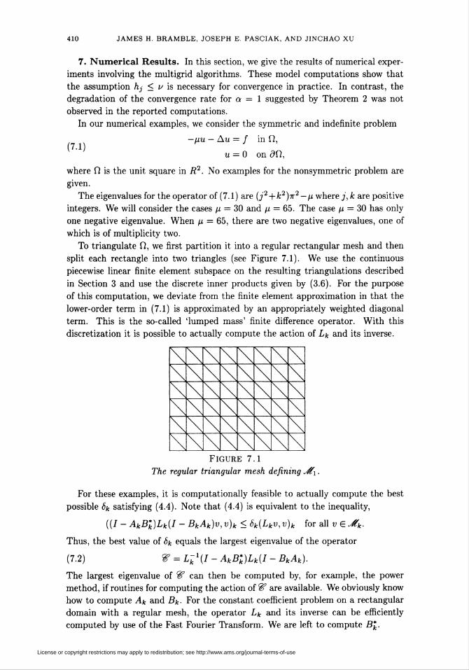
To triangulate fi, we first partition it into a regular rectangular mesh and then
split each rectangle into two triangles (see Figure 7.1). We use the continuous
piecewise linear finite element subspace on the resulting triangulations described
in Section 3 and use the discrete inner products given by (3.6). For the purpose
of this computation, we deviate from the finite element approximation in that the
lower-order term in (7.1) is approximated by an appropriately weighted diagonal
term. This is the so-called 'lumped mass' finite difference operator. With this
discretization it is possible to actually compute the action of Lk and its inverse.
Figure 7.1
The regular triangular mesh defining J?i.
For these examples, it is computationally feasible to actually compute the best
possible <5fc satisfying (4.4). Note that (4.4) is equivalent to the inequality,
((7 - AkB*k)Lk(I - BkAk)v, v)k < 6k(Lkv, v)k for all v E y£k-
Thus, the best value of 6k equals the largest eigenvalue of the operator
(7.2) W = Lkl(I-AkB*k)Lk(I-BkAk).
The largest eigenvalue of W can then be computed by, for example, the power
method, if routines for computing the action of W are available. We obviously know
how to compute Ak and Bk ■ For the constant coefficient problem on a rectangular
domain with a regular mesh, the operator Lk and its inverse can be efficiently
computed by use of the Fast Fourier Transform. We are left to compute Bk.
License or copyright restrictions may apply to redistribution; see http://www.ams.org/journal-terms-of-use
MULTIGRID ALGORITHMS FOR ELLIPTIC PROBLEMS 411
For a symmetric problem, the operator T?£ is also a multigrid operator and is
given by the following algorithm [18]:
Algorithm for computing B*k. Let B* : Jüj h-> J?j denote the adjoint of A~l.
Assume that B\_x : Jtk-\ *-> -^it-i has been defined and define Bkg for g E Jfk
as follows:
(I) Set q° = 0.
(II) Define z° = qp where ql, for i — 1,2,... ,p, is defined by
q'= q'-1 + B*k_i[Ik-ig - Ak-iq1-1}.
(Ill) For 1 = 1,... ,m(k), define
xl=xl-l+p-k2A*k(g-Akx1-1).
Arguments similar to those leading to (4.3) imply that the operator Bk defined by
(I)—(III) satisfies the equation
(7.3) 7 - B*kAk = K™{k)[(I - Pk-i) + (I - Bl_xAk-i)pPk-i}-
A straightforward mathematical induction argument using (7.3) and the symmetry
of Ak implies that the operator defined by (I)—(III) is the adjoint of Bk.
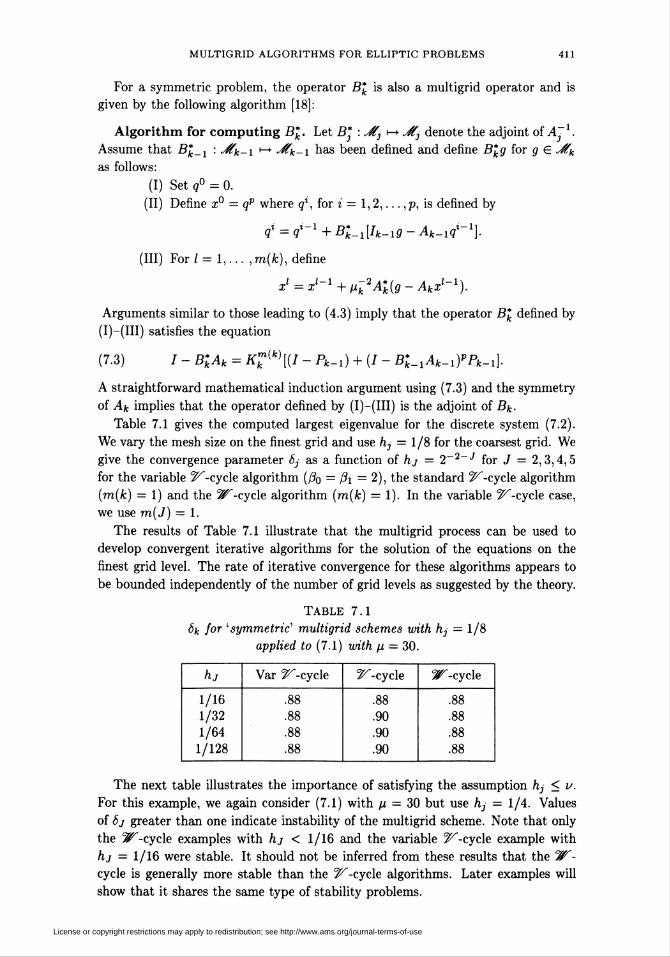
Table 7.1 gives the computed largest eigenvalue for the discrete system (7.2).
We vary the mesh size on the finest grid and use h3 = 1/8 for the coarsest grid. We
give the convergence parameter 6j as a function of hj = 2~2~J for J = 2,3,4,5
for the variable ^"-cycle algorithm (ßo = ßi = 2), the standard ^-cycle algorithm
(m(fc) = 1) and the W-cyc\e algorithm (m(k) = 1). In the variable 2^-cycle case,
we use m(J) = 1.
The results of Table 7.1 illustrate that the multigrid process can be used to
develop convergent iterative algorithms for the solution of the equations on the
finest grid level. The rate of iterative convergence for these algorithms appears to
be bounded independently of the number of grid levels as suggested by the theory.
TABLE 7.1
6k for 'symmetric' multigrid schemes with hj = 1/8
applied to (7.1) with p = 30.
h.,
1/16
1/321/641/128
Var 2^-cycle
.88
2^-cycle
.90
.90
.90
3T-cycle
.88
The next table illustrates the importance of satisfying the assumption hj < v.
For this example, we again consider (7.1) with p = 30 but use hj = 1/4. Values
of 6j greater than one indicate instability of the multigrid scheme. Note that only
the 3F-cycle examples with hj < 1/16 and the variable 2^-cycle example with
hj = 1/16 were stable. It should not be inferred from these results that the W-
cycle is generally more stable than the 2^-cycle algorithms. Later examples will
show that it shares the same type of stability problems.
License or copyright restrictions may apply to redistribution; see http://www.ams.org/journal-terms-of-use
412 JAMES H. BRAMBLE, JOSEPH E. PASCIAK, AND JINCHAO XU
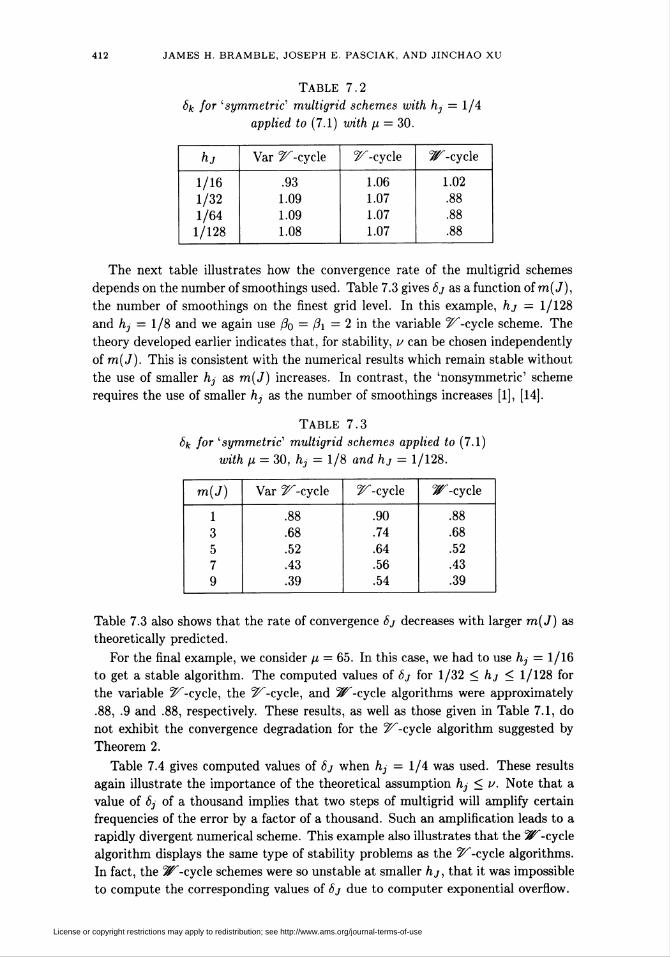
TABLE 7.2
6k for 'symmetric' multigrid schemes with hj = 1/4
applied to (7.1) with p = 30.
h.,
1/161/321/641/128
Var ^-cycle
.931.091.091.08
2^-cycle
1.061.071.071.07
^-cycle
1.02.88
The next table illustrates how the convergence rate of the multigrid schemes
depends on the number of smoothings used. Table 7.3 gives 6j as a function of m(J),
the number of smoothings on the finest grid level. In this example, hj = 1/128
and hj = 1/8 and we again use ßo = ß\ = 2 in the variable ^-cycle scheme. The
theory developed earlier indicates that, for stability, v can be chosen independently
of m(J). This is consistent with the numerical results which remain stable without
the use of smaller h3 as m(J) increases. In contrast, the 'nonsymmetric' scheme
requires the use of smaller h3 as the number of smoothings increases [1], [14].
TABLE 7.3
¿fc for 'symmetric1 multigrid schemes applied to (7.1)
with p = 30, hj = 1/8 and hj = 1/128.
m(J) Var ^-cycle
.68
.52
.43
.39
2^-cycle
.90
.74
.64
.56
.54
^"-cycle
.68
.52
.43
.39
Table 7.3 also shows that the rate of convergence 6j decreases with larger m(J) as
theoretically predicted.
For the final example, we consider p = 65. In this case, we had to use hj — 1/16
to get a stable algorithm. The computed values of 6j for 1/32 < hj < 1/128 for
the variable 2^"-cycle, the 2^-cycle, and ^"-cycle algorithms were approximately
.88, .9 and .88, respectively. These results, as well as those given in Table 7.1, do
not exhibit the convergence degradation for the ^-cycle algorithm suggested by
Theorem 2.
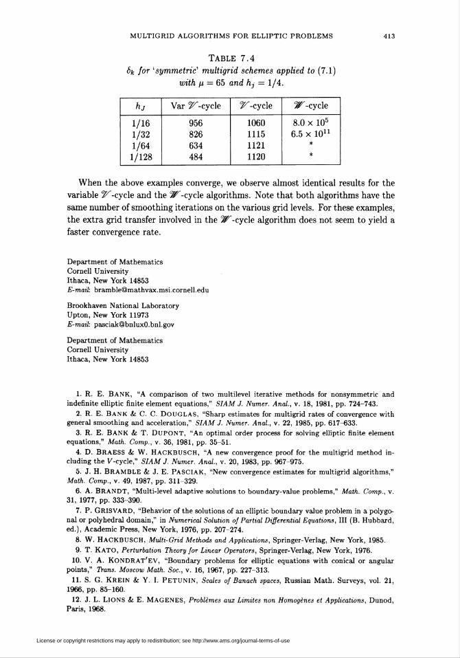
Table 7.4 gives computed values of 6j when h3 = 1/4 was used. These results
again illustrate the importance of the theoretical assumption hj < v. Note that a
value of 8j of a thousand implies that two steps of multigrid will amplify certain
frequencies of the error by a factor of a thousand. Such an amplification leads to a
rapidly divergent numerical scheme. This example also illustrates that the ^"-cycle
algorithm displays the same type of stability problems as the 2^-cycle algorithms.
In fact, the 3F-cycle schemes were so unstable at smaller hj, that it was impossible
to compute the corresponding values of 6j due to computer exponential overflow.
License or copyright restrictions may apply to redistribution; see http://www.ams.org/journal-terms-of-use
MULTIGRID ALGORITHMS FOR ELLIPTIC PROBLEMS 413
TABLE 7.4
6k for 'symmetric'1 multigrid schemes applied to (7.1)
with p — 65 and hj = 1/4.
1/161/321/641/128
Var ^"-cycle
956826634484
2^-cycle
10601115
11211120
^-cycle
8.0 x 10⁵
6.5 x 10¹¹
When the above examples converge, we observe almost identical results for the
variable J^-cycle and the ^-cycle algorithms. Note that both algorithms have the
same number of smoothing iterations on the various grid levels. For these examples,
the extra grid transfer involved in the ^"-cycle algorithm does not seem to yield a
faster convergence rate.
Department of Mathematics
Cornell University
Ithaca, New York 14853
E-mail: [email protected]
Brookhaven National Laboratory
Upton, New York 11973
E-mail: [email protected]
Department of Mathematics
Cornell University
Ithaca, New York 14853
1. R. E. BANK, "A comparison of two multilevel iterative methods for nonsymmetric and
indefinite elliptic finite element equations," SIAM J. Numer. Anal., v. 18, 1981, pp. 724-743.
2. R. E. BANK & C. C. DOUGLAS, "Sharp estimates for multigrid rates of convergence with
general smoothing and acceleration," SIAM J. Numer. Anal, v. 22, 1985, pp. 617-633.
3. R. E. BANK & T. DUPONT, "An optimal order process for solving elliptic finite element
equations," Math. Comp., v. 36, 1981, pp. 35-51.
4. D. BRAESS & W. HACKBUSCH, "A new convergence proof for the multigrid method in-
cluding the V-cycle," SIAM J. Numer. Anal., v. 20, 1983, pp. 967-975.
5. J. H. BRAMBLE & J. E. Pasciak, "New convergence estimates for multigrid algorithms,"
Math. Comp., v. 49, 1987, pp. 311-329.
6. A. BRANDT, "Multi-level adaptive solutions to boundary-value problems," Math. Comp., v.
31, 1977, pp. 333-390.
7. P. GriSVARD, "Behavior of the solutions of an elliptic boundary value problem in a polygo-
nal or polyhedral domain," in Numerical Solution of Partial Differential Equations, III (B. Hubbard,
ed.), Academic Press, New York, 1976, pp. 207-274.
8. W. HACKBUSCH, Multi-Grid Methods and Applications, Springer-Verlag, New York, 1985.
9. T. KATO, Perturbation Theory for Linear Operators, Springer-Verlag, New York, 1976.
10. V. A. Kondrat'ev, "Boundary problems for elliptic equations with conical or angular
points," Trans. Moscow Math. Soc, v. 16, 1967, pp. 227-313.
11. S. G. KREIN Si Y. I. PETUNIN, Scales of Banach spaces, Russian Math. Surveys, vol. 21,1966, pp. 85-160.
12. J. L. LIONS & E. MAGENES, Problèmes aux Limites non Homogènes et Applications, Dunod,
Paris, 1968.
License or copyright restrictions may apply to redistribution; see http://www.ams.org/journal-terms-of-use
414 JAMES H. BRAMBLE, JOSEPH E. PASCIAK, AND JINCHAO XU
13. J. F. MAITRE & F. MUSY, "Algebraic formalization of the multigrid method in the symmet-
ric and positive definite case—A convergence estimation for the V-cycle," in Multigrid Methods for
Integral and Differential Equations (D. J. Paddon and H. Holstein, eds.), Clarendon Press, Oxford,
1985.14. J. MANDEL, "Multigrid convergence for nonsymmetric, indefinite variational problems and
one smoothing step," in Proc. Copper Mtn. Conf. Multigrid Methods, Appl. Math. Comput., 1986,
pp. 201-216.15. J. MANDEL, Algebraic Study of Multigrid Methods for Symmetric, Definite Problems. (Preprint.)
16. J. MANDEL, S. F. McCORMICK & J. RUGE, An Algebraic Theory for Multigrid Methods for
Variational Problems. (Preprint.)
17. S. F. McCORMICK, "Multigrid methods for variational problems: Further results," SIAM
J. Numer. Anal, v. 21, 1984, pp. 255-263.18. S. F. McCORMICK, "Multigrid methods for variational problems: General theory for the
V-cycle," SIAM J. Numer. Anal, v. 22, 1985, pp. 634-643.19. J. NEÖAS, Les Méthodes Directes en Théorie des Equations Elliptiques, Academia, Prague,
1967.20. A. H. SCHATZ, "An observation concerning Ritz-Galerkin methods with indefinite bilinear
forms," Math. Comp., v. 28, 1974, pp. 959-962.21. H. YSERENTANT, "The convergence of multi-level methods for solving finite-element equa-
tions in the presence of singularities," Math. Comp., v. 47, 1986, pp. 399-409.
License or copyright restrictions may apply to redistribution; see http://www.ams.org/journal-terms-of-use