The Agricultural Innovation Process:

Research and Technology Adoption in a ChangingAgricultural Sector

(For the Handbook of Agricultural Economics)

David Sunding and David Zilberman

David Sunding is Cooperative Extension Specialist, Department of Agricultural andResource Economics, University of California at Berkeley

David Zilberman is Professor, Department of Agricultural and Resource Economics,

University of California at Berkeley

Revised January , 2000

Abstract: The chapter reviews the generation and adoption of new technologies in the

agricultural sector. The first section describes models of induced innovation andexperimentation, considers the political economy of public investments in agriculturalresearch, and addresses institutions and public policies for managing innovation activity.

The second section reviews the economics of technology adoption in agriculture.Threshold models, diffusion models, and the influence of risk, uncertainty, and dynamicfactors on adoption are considered. The section also describes the influence of

institutions and government interventions on adoption. The third section outlines futureresearch and policy challenges.

2

Keywords: innovation, diffusion, adoption, technology transfer, intellectual property

David Sunding: tel: 510-642-8229; fax: 510-643-8911; email: sunding@are.berkeley.edu.

David Zilberman: tel: 510-642-6570; fax: 510-643-8911; email: zilber@are.berkeley.edu.

1

The Agricultural Innovation Process:

Research and Technology Adoption in a ChangingAgricultural Sector

Technological change has been a major factor shaping agriculture in the last 100 years

[Schultz (1964); Cochrane (1979)]. A comparison of agricultural production patterns in

the United States at the beginning (1920) and end of the century (1995) shows that

harvested cropland has declined (from 350 to 320 million acres), the share of the

agricultural labor force has decreased substantially (from 26 to 2.6 percent), and the

number of people now employed in agriculture has declined (9.5 million in 1920 vs. 3.3

million in 1995); yet agricultural production in 1995 was 3.3 times greater than in 1920

[United States Bureau of the Census (1975, 1980, 1998)]. Internationally, tremendous

changes in production patterns have occurred. While world population more than

doubled between 1950 and 1998 (from 2.6 to 5.9 billion), grain production per person has

increased by about 12 percent, and harvested acreage per person has declined by half

[Brown, Gardner, and Halweil (1999)]. These figures suggest that productivity has

increased and agricultural production methods have changed significantly.

2

There is a large amount of literature investigating changes in productivity,1 which

will not be addressed here. Instead this chapter presents an overview of agricultural

economic research on innovations—the basic elements of technological and institutional

change. Innovations are defined here as new methods, customs, or devices used to

perform new tasks.

The literature on innovation is diverse and has developed its own vocabulary. We

will distinguish between two major research lines: research on innovation generation and

research on the adoption and use of innovation. Several categories of innovations have

been introduced to differentiate policies or modeling. For example, the distinction

between innovations that are embodied in capital goods or products (such as tractors,

fertilizers, and seeds) and those that are disembodied (e.g., integrated pest management

schemes) is useful for directing public investment in innovation generation. Private

parties are less likely to invest in generating disembodied innovations because of the

difficulty in selling the final product, so that is an area for public action. Private

investment in the generation of embodied innovations requires appropriate institutions for

intellectual property rights protection, as we will see below.

The classification of innovations according to form is useful for considering

policy questions and understanding the forces behind the generation and adoption of

innovations. Categories in this classification include mechanical innovations (tractors

1 See Mundlak (1997), Ball et al. (1997), and Antle and McGuckin (1993).

3

and combines), biological innovations (new seed varieties), chemical innovations

(fertilizers and pesticides), agronomic innovations (new management practices),

biotechnological innovations, and informational innovations that rely mainly on computer

technologies. Each of these categories may raise different policy questions. For

example, mechanical innovations may negatively affect labor and lead to farm

consolidation. Chemical and biotechnological innovations are associated with problems

of public acceptance and environmental concerns. We will argue later that economic

forces as well as the state of scientific knowledge affect the form of innovations that are

generated and adopted in various locations.

Another categorization of innovation according to form distinguishes between

process innovations (e.g., a way to modify a gene in a plant) and product innovations

(e.g., a new seed variety). The ownership of rights to a process that is crucial in

developing an important product may be a source of significant economic power. We

will see how intellectual property rights and regulations affect the evolution of innovation

and the distribution of benefits derived from them.

Innovations can also be distinguished by their impacts on economic agents and

markets which affect their modeling; these categories include yield-increasing, cost-

reducing, quality-enhancing, risk-reducing, environmental-protection increasing, and

shelf-life enhancing. Most innovations fall into several of these categories. For example,

a new pesticide may increase yield, reduce economic risk, and reduce environmental

4

protection. The analysis of adoption or the impact of risk-reducing innovations may

require the incorporation of a risk-aversion consideration in the modeling framework,

while investigating the economics of a shelf-life enhancing innovation may require a

modeling framework that emphasizes inter-seasonal dynamics.

Three sections on the generation of innovations follow in Part I. The first

introduces results of induced innovation models and the role of economic forces in

triggering innovations; the second presents a political-economic framework for

government financing of innovations; and the third addresses various institutions and

policies for managing innovation activities. Part II discusses the adoption of innovations

and includes four sections. The first section considers threshold models and models of

diffusion as a process of imitation; the second presents adoption under uncertainty; the

third addresses dynamic considerations on adoption; and the last two sections deal with

the impact of institutional and policy constraints on adoption. Part III addresses future

directions.

5

I. GENERATION OF INNOVATION

Induced Innovations

There are several stages in the generation of innovations. These stages are depicted in

Figure 1. The first stage is discovery, characterized by the emergence of a concept or

results that establish the innovation. A second essential stage is development, where the

discovery moves from the laboratory to the field, and is scaled up, commercialized, and

integrated with other elements of the production process. In cases of patentable

innovations, between the time of discovery and development there may also be a stage

where there is registration for a patent. If the innovation is embodied, once it is

developed it has to be produced and, finally, marketed. For embodied innovations, the

marketing stage consists of education, demonstration, and sales. Only then does adoption

occur.

Insert Figure 1

Some may hold the notion that new discoveries are the result of inspiration

occurring randomly without a strong link to physical reality. While that may sometimes

be the case, Hayami and Ruttan (1985) formalized and empirically verified their theory of

induced innovations that closely linked the emergence of innovations with economic

conditions. They argued that the search for new innovations is an economic activity that

6

is significantly affected by economic conditions. New innovations are more likely to

emerge in response to scarcity and economic opportunities. For example, labor shortages

will induce labor-saving technologies. Environmental-friendly techniques are likely to be

linked to the imposition of strict environmental regulation. Drip irrigation and other

water-saving technologies are often developed in locations where water constraints are

binding, such as Israel and the California desert. Similarly, food shortages or high prices

of agricultural commodities will likely lead to the introduction of a new high-yield

variety, and perceived changes in consumer preferences may provide the background for

new innovations that modify product quality.

The work of Boserup (1965) and Binswanger and McIntire (1987) on the

evolution of agricultural systems supports the induced-innovation hypothesis. Early

human groups, consisting of a relatively small number of members who could roam large

areas of land, were hunters and gatherers. An increase in population led to the evolution

of agricultural systems. In tropical regions where population density was still relatively

small, farmers relied on slash and burn systems. The transition to more intensive farming

systems that used crop rotation and fertilization occurred as population density increased

even further. The need to overcome diseases and to improve yields led to the

development of innovations in pest control and breeding, and the evolution of the

agricultural systems we are familiar with. The work of Berck and Perloff (1985) suggests

that the same phenomena may occur with seafood. An increased demand for fish and

7

expanded harvesting may lead to the depletion of population and a rise in harvesting

costs, and thus trigger economic incentives to develop alternative aquaculture and

mariculture for the provision of seafood.

While scarcity and economic opportunities represent potential demand that is, in

most cases, necessary for the emergence of new innovations, a potential demand is not

sufficient for inducing innovations. In addition to demand, the emergence of new

innovations requires technical feasibility and new scientific knowledge that will provide

the technical base for the new technology. Thus, in many cases, breakthrough knowledge

gives rise to new technologies. Finally, the potential demand and the appropriate

knowledge base are integrated with the right institutional setup, and together they provide

the background for innovation activities. These ideas can be demonstrated by an

overview of some of the major waves of innovations that have affected U.S. agriculture

in the last 150 years.

New innovations currently are linked with discoveries of scientists in universities

or firms. However, in the past, practitioners were responsible for most breakthroughs.

Over the years, the role of research labs in producing new innovations has drastically

increased, but field experience is still very important in inspiring innovations. John

Deere, who invented the steel plow, was a farmer. This innovation was one of a series of

mechanical innovations that were of crucial importance to the westward expansion of

U.S. agriculture in the nineteenth century. At the time, the United States had vast tracts

8

of land and a scarcity of people; this situation induced a wide variety of labor-saving

innovations such as the thresher, several types of mechanical harvesters, and later the

tractor.

Olmstead and Rhode (1993) argue that demand considerations represented by the

induced-innovation hypothesis do not provide the sole explanation for the introduction of

new technologies. They conclude that during the nineteenth century, when farm

machinery (e.g., the reaper) was introduced in the United States, land prices increased

relative to labor prices, which seems to contradict the induced-innovation hypothesis. As

settlement of the West continued and land became more scarce, land prices may have

risen relative to labor, but the cost of labor in America relative to other regions was high,

and that provided the demand for mechanical innovations. Olmstead and Rhode (1993)

argue that other factors also affected the emergence of these innovations, including the

expansion of scientific knowledge in metallurgy and mechanics (e.g., the Bessemer

process for the production of steel, and the invention of various types of mechanical

engines), the establishment of the input manufacturing industry, and the interactive

relationship between farmers and machinery producers.

The infrastructure that was established for the refinement, development, and

marketing of the John Deere plow was later used for a generation of other innovations,

and the John Deere Company became the world’s leading manufacturer of agricultural

mechanical equipment. It was able to establish its own research and development (R&D)

9

infrastructure for new mechanical innovations, had enough financial leverage to buy the

rights to develop other discoveries, and subsequently took over smaller companies that

produced mechanical equipment that complemented its own. This pattern of evolution,

where an organization is established to generate fundamental innovations of a certain

kind, and then later expands to become a leading industrial manufacturer, is repeated in

other situations in and out of agriculture.

It seems that during the settlement period of the nineteenth century, most of the

emphasis was on mechanical innovation. Cochrane (1979) noted that yield per acre did

not change much during the nineteenth century, but the production of U.S. agriculture

expanded drastically as the land base expanded. However, Olmstead and Rhode (1993)

suggest that even during that period there was heavy emphasis on biological innovation.

Throughout the settlement period, farmers and scientists, who were part of research

organizations such as the Agricultural Research Service (ARS) of the United States

Department of Agriculture (USDA), and the experiment stations at the land-grant

universities in the United States, experimented with new breeds, both domestic and

imported, and developed new varieties that were compatible with the agro-climatic

conditions of the newly settled regions. These efforts maintained per-acre yields.

Once most of the arable agricultural land of the continental United States was

settled, expansion of agricultural production was feasible mostly through increases in

yields per acre. The recognition of this reality and the basic breakthroughs in genetics

10

research in the nineteenth century increased support for research institutions in their

efforts to generate yield-increasing innovations. Most of the developed countries

established agricultural research institutions. After World War II, a network of

international research centers was established to provide agricultural innovations for

developing countries. The establishment of these institutions reflected the recognition

that innovations are products of R&D activities, and that the magnitude of these activities

is affected by economic incentives.

Economic models have been constructed to explain patterns of investment in

R&D activities and the properties of the emerging innovations. Evenson and Kislev

(1976) developed a production function of research outcomes particularly appropriate for

crop and animal breeding. In breeding activities, researchers experiment with a large

number of varieties to find the one with the highest yield. The outcome of research

efforts depends on a number of plots. In their model, the yield per acre of a crop is a

random variable that can assume numerous values. Each experiment is a sampling of a

value of this random variable and, if experiments are conducted, the experiment with the

highest value will be chosen. Let Yn be yield per acre of the nth experiment and n

assumes value from 1 to N. The outcome of n experiments is YN* = max Y1 ,...,YN{ }. YN

* is

the maximum value of the n experiment. Each Yn can assume the value in the range of

11

0,YX( ) with probability density g Yn( ) so that Ymaxg Yn( )dYn = 1. The outcome of research

on N plots YN* is a random variable with the expected value µ N( ) = E max

n =1,NYn{ } .

Evenson and Kislev (1976) showed that the expected value of YN* increases with

the number of the experiment, i.e., µN =∂EY∗

∂N> 0, µNN =

∂2 EY∗

∂N2 < 0 . As in Evenson

and Kislev, consider the determination of optimal research levels when a policymaker’s

objective is to maximize net expected gain from research. Assume that the research

improves the productivity of growers in a price-taking industry with output price P and

acreage L. The new innovation is adopted fully and does not require extra research cost.

The optimal research program is determined by solving

maxN

PL U N( )( ) − C(N) .

The first-order condition is

PL µN − CN = 0, (1)

where CN is the cost of the Nth research plot, and CN > 0, CNN > 0. Condition (1)

implies that the optimal number of experiments is such that the expected value of the

marginal experiment, PLµN( ) , equals the marginal cost of experiments, CN( ) .

Furthermore, the analysis can show that the research effort increases with the size of the

region, ∂N ∂L > 0( ) , and the scarcity of the product, ∂N* ∂P > 0( ) . Similarly, lower

research costs will lead to more research effort.

12

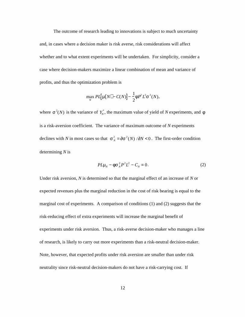
The outcome of research leading to innovations is subject to much uncertainty

and, in cases where a decision maker is risk averse, risk considerations will affect

whether and to what extent experiments will be undertaken. For simplicity, consider a

case where decision-makers maximize a linear combination of mean and variance of

profits, and thus the optimization problem is

maxN

PL µ N( ) − C(N)[ ]−1

2φP2 L2σ 2(N),

where σ 2(N) is the variance of YN*, the maximum value of yield of N experiments, and φ

is a risk-aversion coefficient. The variance of maximum outcome of N experiments

declines with N in most cases so that σ N2 = ∂σ 2(N) /∂N < 0 . The first-order condition

determining N is

PLµN − φσ N2 P2L2 − CN = 0 . (2)

Under risk aversion, N is determined so that the marginal effect of an increase of N or

expected revenues plus the marginal reduction in the cost of risk bearing is equal to the

marginal cost of experiments. A comparison of conditions (1) and (2) suggests that the

risk-reducing effect of extra experiments will increase the marginal benefit of

experiments under risk aversion. Thus, a risk-averse decision-maker who manages a line

of research, is likely to carry out more experiments than a risk-neutral decision-maker.

Note, however, that expected profits under risk aversion are smaller than under risk

neutrality since risk-neutral decision-makers do not have a risk-carrying cost. If

13

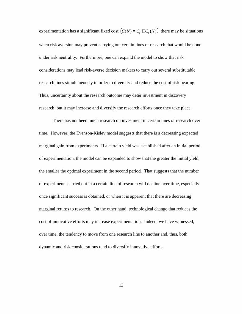
experimentation has a significant fixed cost C(N) = C0 + C1 (N)( ) , there may be situations

when risk aversion may prevent carrying out certain lines of research that would be done

under risk neutrality. Furthermore, one can expand the model to show that risk

considerations may lead risk-averse decision makers to carry out several substitutable

research lines simultaneously in order to diversify and reduce the cost of risk bearing.

Thus, uncertainty about the research outcome may deter investment in discovery

research, but it may increase and diversify the research efforts once they take place.

There has not been much research on investment in certain lines of research over

time. However, the Evenson-Kislev model suggests that there is a decreasing expected

marginal gain from experiments. If a certain yield was established after an initial period

of experimentation, the model can be expanded to show that the greater the initial yield,

the smaller the optimal experiment in the second period. That suggests that the number

of experiments carried out in a certain line of research will decline over time, especially

once significant success is obtained, or when it is apparent that there are decreasing

marginal returns to research. On the other hand, technological change that reduces the

cost of innovative efforts may increase experimentation. Indeed, we have witnessed,

over time, the tendency to move from one research line to another and, thus, both

dynamic and risk considerations tend to diversify innovative efforts.

14

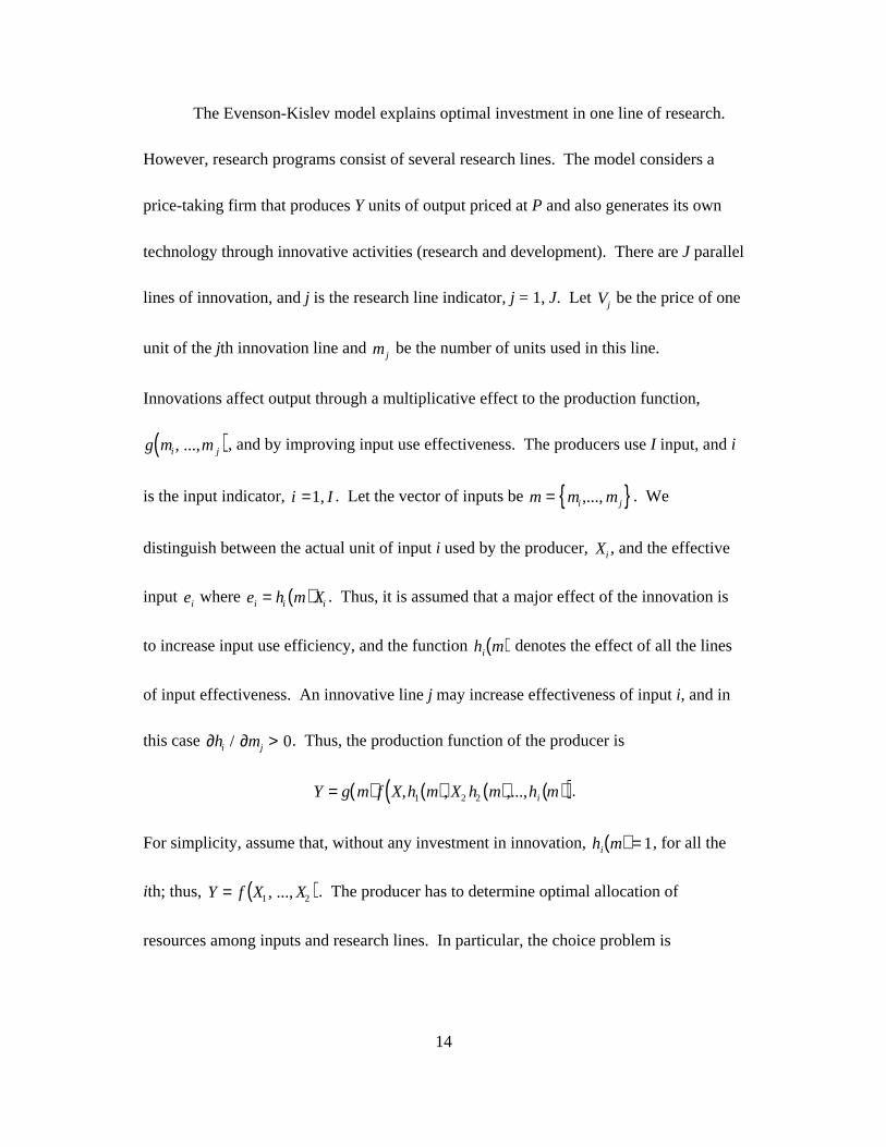
The Evenson-Kislev model explains optimal investment in one line of research.

However, research programs consist of several research lines. The model considers a

price-taking firm that produces Y units of output priced at P and also generates its own

technology through innovative activities (research and development). There are J parallel

lines of innovation, and j is the research line indicator, j = 1, J. Let Vj be the price of one

unit of the jth innovation line and m j be the number of units used in this line.

Innovations affect output through a multiplicative effect to the production function,

g mi , ...,m j( ), and by improving input use effectiveness. The producers use I input, and i

is the input indicator, i =1, I . Let the vector of inputs be m = mi ,..., m j{ }. We

distinguish between the actual unit of input i used by the producer, Xi , and the effective

input ei where ei = hi m( )Xi . Thus, it is assumed that a major effect of the innovation is

to increase input use efficiency, and the function hi m( ) denotes the effect of all the lines

of input effectiveness. An innovative line j may increase effectiveness of input i, and in

this case ∂hi / ∂mj > 0. Thus, the production function of the producer is

Y = g m( ) f X,h1 m( ), X2 h2 m( ),...,hi m( )( ).

For simplicity, assume that, without any investment in innovation, hi m( ) = 1, for all the

ith; thus, Y = f X1 , ..., X2( ). The producer has to determine optimal allocation of

resources among inputs and research lines. In particular, the choice problem is

15

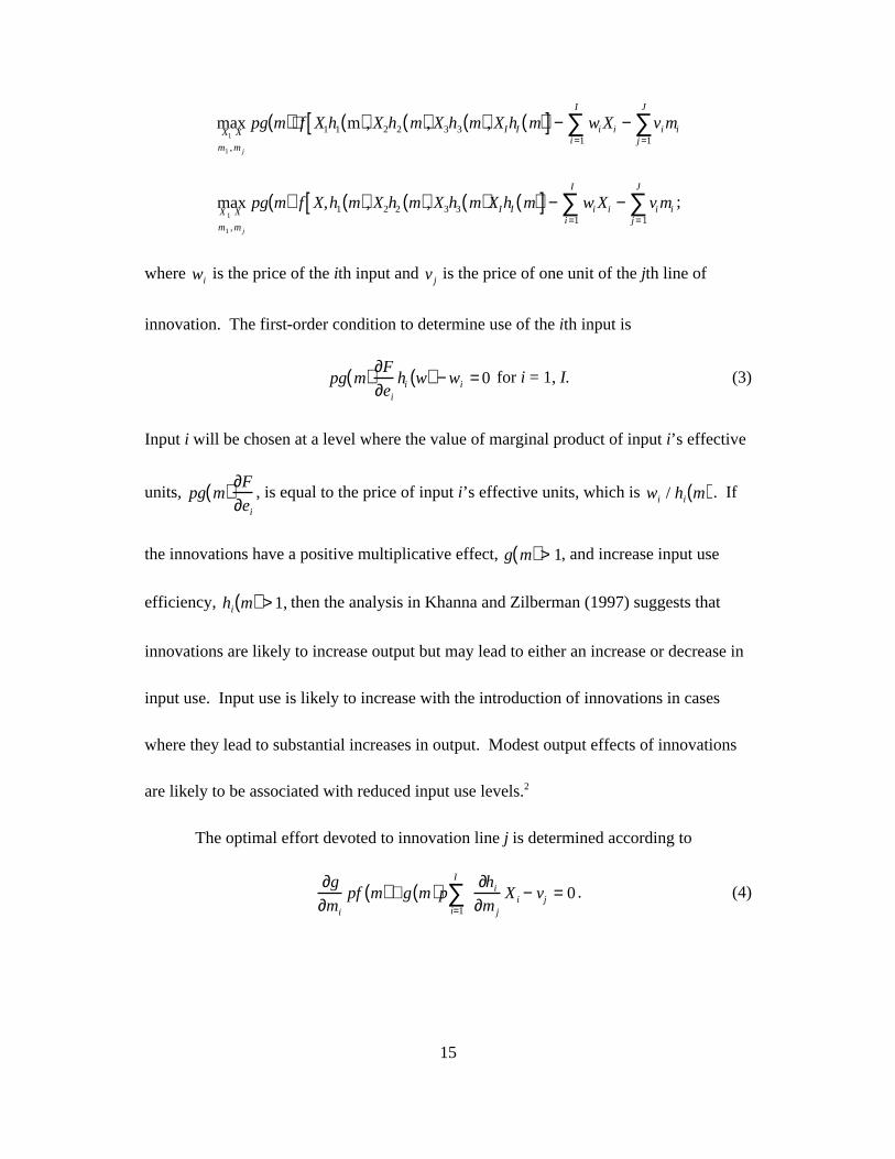
maxX1 X

m1 , m j

pg m( )⋅ f X1h1 m( ), X2h2 m( ), X3h3 m( ), XIhI m( )[ ] − wii =1

I

∑ Xi − vij =1

J

∑ mi

maxX 1 X

m1 , m j

pg m( ) f X,h1 m( ), X2h2 m( ), X3h3 m( )XIhI m( )[ ] − wii =1

I

∑ Xi − vij = 1

J

∑ mi ;

where wi is the price of the ith input and v j is the price of one unit of the jth line of

innovation. The first-order condition to determine use of the ith input is

pg m( ) ∂F

∂ei

hi w( ) − wi = 0 for i = 1, I. (3)

Input i will be chosen at a level where the value of marginal product of input i’s effective

units, pg m( ) ∂F

∂ei

, is equal to the price of input i’s effective units, which is wi / hi m( ) . If

the innovations have a positive multiplicative effect, g m( ) > 1, and increase input use

efficiency, hi m( ) > 1, then the analysis in Khanna and Zilberman (1997) suggests that

innovations are likely to increase output but may lead to either an increase or decrease in

input use. Input use is likely to increase with the introduction of innovations in cases

where they lead to substantial increases in output. Modest output effects of innovations

are likely to be associated with reduced input use levels.2

The optimal effort devoted to innovation line j is determined according to

∂g

∂mi

pf m( ) + g m( )p∂hi

∂m j

X ii=1

I

∑ − vj = 0 . (4)

16

Let the elasticity of the multiplicative effect of innovation with respect to the level of

innovation j be denoted by εm j

g =∂g

∂m j

mj

g m( ), and let the elasticity of input i’s

effectiveness coefficient, with respect to the level of innovation j, be εm j

hi =∂hi

∂m j

mj

hi

.

Using (3), the first order condition (4) becomes

PY εm j

g + Sii=1

I

∑ εmj

hi

− m jvj = 0 , (5)

where Si = wi Xi / PY is the revenue share of input i. Condition (5) states that, under

optimal resource allocation, the expenditure share (in total revenue of innovation line j)

will be equal to the sum of elasticities of the input effectiveness, with respect to research

line j, and the elasticity of the multiplicative output coefficient with respect to this

research line. This condition suggests that more resources are likely to be allocated to

research lines with higher productivity effects that mostly impact inputs with higher

expenditure shares that have a relatively lower cost.3

Risk considerations provide part of the explanation for such diversification, but

whether innovations are complements or substitutes may also be a factor. When the

tomato harvester was introduced in California, it was accompanied by the introduction of

a new complementary tomato variety [de Janvry, LeVeen, and Runsten (1981)].

2 Khanna and Zilberman (1997) related the impact of technological change on input use to the curvature ofthe production function. If marginal productivity of ei declines substantially with an increase in ei , the

output effects are restricted and innovation leads to reduced input use.3 Binswanger (1974) proves these assertions under a very narrow set of conditions.

17

McGuirk and Mundlak’s (1991) analysis of the introduction of high-yield “green

revolution” varieties in the Punjab shows that it was accompanied by the intensification

of irrigation and fertilization practices.

The induced innovation hypothesis can be expanded to state that investment in

innovative activities is affected by shadow prices implied by government policies and

regulation. The tomato harvester was introduced following the end of the Bracero

Program, whose termination resulted in reduced availability of cheap immigrant workers

for California and Florida growers. Environmental concerns and regulation have led to

more intensive research and alternatives for the widespread use of chemical pesticides.

For example, they have contributed to the emergence of integrated pest management

strategies and have prompted investment in biological control and biotechnology

alternatives to chemical pesticides.

Models of induced innovation should be expanded to address the spatial

variability of agricultural production. The heterogeneity of agriculture and its

vulnerability to random events such as changes in weather and pest infestation led to the

development of a network of research stations. A large body of agricultural research has

been aimed at adaptive innovations that develop practices and varieties that are

appropriate for specific environmental and climatic conditions. The random emergence

of new diseases and pests led to the establishment of research on productivity

18

maintenance aimed at generating new innovations in response to adverse outcomes

whenever they occurred.

The treatment of the mealybug in the cassava in Africa is a good example of

responsive research. Cassava was brought to Africa from South America 300 years ago

and became a major subsistence crop. The mealybug, one of the pests of cassava in

South America, was introduced to Africa and reduced yields by more than 50 percent in

1983–84; without treatment, the damage could have had a devastating effect on West

Africa [Norgaard (1988)]. The International Institute of Tropical Agriculture launched a

research program which resulted in the introduction of a biological control in the form of

a small wasp, E lopezi, that is a natural enemy of the pest in South America. Norgaard

estimated the benefit/cost ratio of this research program to be 149 to 1, but his calculation

did not take into account the cost of the research that established the methodology of

biological control, and the fixed cost associated with maintaining the infrastructure to

respond to the problem.

Induced innovation models such as Binswanger’s (1974) are useful in linking the

evolution of innovations to prices, costs, and technology. However, they ignore some of

the important details that characterize the system leading to agricultural innovations.4

Typically, new agricultural technologies are not used by the entities that develop them

4 The Binswanger model (1974) is very closely linked to the literature on quantifying sources ofproductivity in agriculture. For an overview of this important body of literature, which benefited fromseminal contributions by Griliches (1957, 1958) and Mundlak, see Antle and McGuckin (1993).

19

(e.g., universities and equipment manufacturers). Different types of entities have their

distinct decision-making procedures that need to be recognized in a more refined analysis

of agricultural innovations. The next subsection will analyze resource allocation for the

development of new innovations in the public sector, and that will be followed by a

discussion of specific institutions and incentives for innovation activities (patents and

intellectual property rights) in the private sector.

Induced innovations by agribusiness apply to innovations beyond the farm gate.

In much of the post World War II period, there has been an excess supply of agricultural

commodities in world markets. This has led to a period of low profitability in agriculture

requiring government support. While increasing food quantity has become less of a

priority, increasing the value added to food products has become a major concern of

agriculture and agribusiness in developed nations. Indeed, that has been the essence of

many of the innovations related to agriculture in the last 30 years. Agribusiness took

advantage of improvements in transportation and weather-controlled technologies that led

to innovations in packing, storage, and shipping. These changes expanded the

availability as well as the quality of meats, fruits, and vegetables; increased the share of

processing and handling in the total food budget; and caused significant changes in the

structure of both food marketing industries and agriculture.

It is important to understand the institutional setup that enables these innovations

to materialize. While there has not been research in this area, it seems that the

20

availability of numerous sources of funding to finance new ventures (e.g., venture capital,

stock markets, mortgage markets, credit lines from buyers) enables the entities that own

the rights to new innovations to change the way major food items are produced,

marketed, and consumed.

Political Economy of Publicly Funded Innovations

Applied R&D efforts are supported by both the public and private sectors because of the

innovations they are likely to spawn. Public R&D efforts are justified by the public-good

nature of these activities and the inability of private companies to capture all the benefits

resulting from farm innovations.

Studies have found consistently high rates of returns (above 20 percent) to public

investment in agricultural research and extension, indicating underinvestment in these

activities [see Alston, Norton, and Pardey (1995); Huffman (1998)]. Analysis of patterns

of public spending for R&D in agriculture shows that federal monies tend to emphasize

research on science and commodities which are grown in several states (e.g., wheat, corn,

rice), while individual states provide much of the public support for innovation-inducing

activities for crops that are specialties of the state (e.g., tomatoes and citrus in Florida,

and fruits and vegetables in California). The process of devolution has also applied to

public research and, over the years, the federal share in public research has declined

relative to the state’s share. Increased concern for environmental and resource

21

management issues over time led to an increase in relative shares of public research

resources allocated to these issues in agriculture [Huffman and Just (1994)].

Many of the studies evaluating returns to public research in agriculture (including

Griliches’ 1957 study on hybrid corn that spawned the literature) rely on partial

equilibrium analysis, depicted in Figure 2.

Insert Figure 2

The model considers an agricultural industry facing a negatively sloped demand curve D.

The initial supply is denoted by S0 , and the initial price and quantity are P0 and Q0 ,

respectively. Research, development, and extension activities led to adoption of an

innovation that shifts supply to S1 , resulting in price reduction to P1, and consumption

gain Q1 .5 The social gain from the innovation is equal to the area A0B0B1 A1 in Figure 2

denoted by G. If the investment leading to the use of the innovation is denoted by I, the

net social gain is NG = G − I , and the social rate of return to appropriate research

development and extension activities is NG I .

The social gain from the innovation is divided between consumers and producers.

In Figure 2, consumer gain is equal to the area P0B0B1P1 . Producer gain is A0FA1B1

because of lower cost and higher sales, but they lose P0B0FP1 because of lower price. If

demand is sufficiently inelastic, producers may actually lose from public research

5 Of course, actual computation requires discounting and aggregation, and benefits over time, and mayrecognize the gradual shift in supply associated with the diffusion process.

22

activities and the innovations that they spawn. Obviously, producers may not support

research expenditures on innovations that may worsen their well being, and distributional

considerations affect public decisions that lead to technological evolution.6

This point was emphasized in Schmitz and Seckler’s (1970) study of the impact

of the introduction of the tomato harvester in California. They showed that society as a

whole gained from the tomato harvester, while farm workers lost from the introduction of

this innovation. The controversy surrounding the tomato harvester [de Janvry, LeVeen,

and Runsten (1981)] led the University of California to de-emphasize research on

mechanical innovations.

De Gorter and Zilberman (1990) introduced a simple model for analyzing

political economic considerations associated with determining public expenditures on

developing new agricultural technologies. Their analysis considers a supply-enhancing

innovation. They consider an industry producing Y units of output. The cost function of

the industry is C (Y, I) and depends on output and investment in R&D where the level is

I. This cost function is well behaved and an increase in I tends to reduce cost at a

decreasing rate ∂c ∂I < 0 , and ∂2c / ∂I2 > 0 and marginal cost of output ∂2c ∂I∂Y < 0 .

Let the cost of investment be denoted by r and the price of output by P. The industry is

6 Further research is needed to understand to what extent farmers take into consideration the long-termdistributional effects of research policy. They may be myopic and support a candidate who favors anyresearch, especially when facing a pest or disease.

23

facing a negative-sloped demand curve, Y = D(P). The gross surplus from consumption

is denoted by the benefit function B(Y) = P(z)dz ,0

Y

∫ where P(Y) is inverse demand.

Social optimum is determined at the levels of Y and I that maximize the net

surplus. Thus, the social optimization problem is

maxY, I

B(Y) − C(Y, I) − rI ,

and the first-order optimality conditions are

∂B

∂Y−

∂C

∂Y= 0 ⇒ P(Y ) =

∂C

∂Y, (6)

and

−∂C

∂I− γ = 0. (7)

Condition (6) is the market-clearing rule in the output market, where price is

equal to marginal cost. Condition (7) states the optimal investment in R&D at a level

where the marginal reduction in production cost because of investment in R&D is equal

to the cost of investment. The function −∂C

∂I reflects a derived demand for supply-

shifting investment and, by our assumptions, reducing the price of investment (γ ) will

increase its equilibrium level. Condition (7) does not likely hold in reality. However, it

provides a benchmark with which to assess outcomes under alternative political

arrangements.

24

De Gorter and Zilberman (1990) argued that the political economic system will

determine both the level of investment in R&D and the share of the burden of financing it

between consumers (taxpayers) and producers. Let Z be the share of public investment in

R&D financed by producers. Thus, Z = 0 corresponds to the case where R&D is fully

financed by taxpayers, and Z = 1 where R&D is fully financed by producers. The latter

case occurs when producers use marketing orders to raise funds to collectively finance

research activities. There are many cases in agriculture where producers compete in the

output market but cooperate in technology development or in the political arena [Guttman

(1978)].

De Gorter and Zilberman (1990) compare outcomes under alternative

arrangements, including the case where producers both determine and finance investment

in R&D. In this case, I is the result of a constrained optimization problem, where

producer surplus, PS = P(Y)Y − C(Y, I), minus investment cost, rI , is maximized subject

to the market-clearing constraint in the output market P(Y) = ∂C / ∂Y . When there is

internal solution, the first-order optimality condition for I is

−∂C

∂I− η = r (8)

where η = −Y∂2C

∂Y∂C1 −

∂2C

∂Y2

/

∂P

∂I

. The optimal solution occurs at a level where

the marginal cost saving due to investment minus the term η , which reflects the loss of

25

revenues because of price reduction, is equal to the marginal investment cost, r. The loss

of revenues because of a price reduction due to the introduction of a supply-enhancing

innovation increases as demand becomes less elastic. A comparison of (8) to (7) suggests

that under-investment in agricultural R&D is likely to occur when producers control its

level and finance it, and the magnitude of the under-investment increases as demand for

the final product becomes less elastic. Below a certain level of demand elasticity, it will

be optimal for producers not to invest in R&D at all. If taxpayers (consumers) pay for

research but producers determine its level, the optimal investment will occur where the

marginal reduction in cost due to the investment is equal to η , the marginal loss in

revenue due to price reduction. When the impact of innovation on price is low (demand

for final product is highly elastic), producer control may lead to over-investment if

producers do not pay for it. However, when η > r , and expansion of supply leads to

significant price reduction, even when taxpayers pay for public agricultural research,

producer determination of its level will lead to under-investment.

The public sector has played a major role in funding R&D activities that have led

to new agricultural innovations, especially innovations that are disembodied or are

embodied but non-shielded. Rausser and Zusman (1991) have argued that choices in

political-economic systems are effectively modeled as the outcome of cooperative games

among parties. Assume that two groups, consumers/taxpayers and producers, are

26

affected by choices associated with investment in the supply-increasing innovation

mentioned above. The political-economic system determines two parameters. The first

is the investment in the innovation (I) and the second is the share of the innovation cost

financed by consumers. Let this share be denoted as z; thus, the consumer will pay zc I( )

for the innovation cost. It is assumed that the investment in the innovation is non-

negative I ≥ 0( ) , but z is unrestricted (z > 1 implies that the producers are actually

subsidized).

The net effects of the investment and finance of innovations on

consumers/taxpayers’ welfare and producers’ welfare are ∆CS I( ) − zc I( ) and

∆PS I( ) − 1 − z( )c I( ), respectively. The choice of the innovation investment and the

sharing coefficients are approximated by the solution to the optimization problem

maxI ,Z

∆CS(I) − zc(I)( )α ∆PS(I) − (1− z )c(I)( )1 −α , (9)

where α is the consumer weight coefficient, 0 ≤ α ≤ 1. The optimization problem (9) (i)

incorporates the objective of the two parties; (ii) leads to outcomes that will not make any

of the parties worse off; (iii) reflects the relative power of the parties (when α is close to

one, consumers dominate decision making but the producers have much of the power

27

when α → 0 ); and (iv) reflects decreasing marginal valuation of welfare gained by most

parties.7

After some manipulations, the solutions to this optimization problem are

presented by

∆CS(I)

∂I+

∂∆PS(1)

∂I=

∂C

∂I; (10)

α1

1 −α1

=∆CS(I) − zc( I)

∆PS(I) − (1− z)c(I). (11)

Equation (10) states that innovation investment will be determined when the sum of the

marginal increase in consumer and producer surplus is equal to the marginal cost of

investment innovation. This rule is equivalent to equating the marginal cost of

innovation investment with its marginal impact on market surplus (since

∆MS = ∆PS + ∆CS ).

Equation (11) states that the shares of two groups in the total welfare gain are

equal to their political weight coefficients. Thus, if α1 is equal to, say, 0.3 and

consumers have 30 percent of the weight in determining the level and distribution of

finance of innovation research, then they will receive 30 percent of the benefit.

Producers will receive the other 70 percent. Equation (9) suggests that the political

weight distribution does not affect the total level of investment in innovation research

7 ∂PG

∂I> 0

∂ 2 PG

∂I2

< 0,∂CS

∂I> 0 ,

∂ 2 CS

∂I2

< 0.

28

that is socially optimal, but only affects the distribution of benefits. If farmers have more

political gain in determining the outcome because of their intense interest in agricultural

policy issues, they will gain much of the benefit from innovation research.

The cooperative game framework is designed to lead to outcomes where both

parties benefit from the action they agree upon. Since both demand and supply

elasticities for many agricultural commodities are relatively low, producer surplus is

likely to decline with expanded innovation research. When these elasticities are

sufficiently low, farmers as a group will directly lose from expanded innovation research

unless compensated. Thus, in certain situations and for some range of products, positive

innovation research is not feasible unless farmers are compensated. This analysis

suggests a strong link between public support for innovation research and programs that

support farm income. In such situations innovation research leads to a significant direct

increase in consumer surplus through increased supplies and a reduction in commodity

prices. It will also result in an increase in farmer subsidies by taxpayers. Thus, for a

range of commodities with low elasticities of output supply and demand,

consumers/taxpayers will finance public research and compensate farmers for their

welfare losses. For commodities where demand is quite elastic, say about 2 or 3, and

both consumers and producers gain significantly from the fruits of innovation research,

both groups will share in financing the research. When demand is very elastic and most

of the gain goes to producers, the separate economic frameworks suggest that they are

29

likely to pay for this research significantly, but if their political weight in the decision is

quite important (α close to 1), they may benefit immensely from the fruits of the

innovation research, but consumers may pay a greater share of the research.

While this political analysis framework is insightful in that it describes the link

between public support for agricultural research and agricultural commodity programs, it

may be off the mark in explaining the public investment in innovation research in

agriculture, since there is a large array of studies that argues that the rate of return for

agricultural research is very high, and thus there is under-investment. One obvious

limitation of the model introduced above is that it assumes that the outcomes of research

innovation are certain. However, there is significant evidence that returns for research

projects are highly skewed. A small number of products may generate most of the

benefits, and most projects may have no obvious outcome at all. This risk consideration

has to be incorporated explicitly in the analysis determining the level of investment in

innovation research. Thus, when consumers consider investment I in innovation

research, they are aware that each investment level generates a distribution of outcome,

and they will consider the expected consumer surplus gain associated with I. Similarly,

producers are aware of the uncertainty involved with innovation research, and they will

consider the expected producer surplus associated with each level in assessing the various

levels of innovation research.

30

Policies and Institutions for Managing Innovation Activities

The theory of induced innovations emphasizes the role of general economic conditions in

shaping the direction of innovation activities. However, the inducement of innovations

also requires specific policies and institutions that provide resources to would-be

innovators and enable them to reap the benefits from their innovations.

Patent protection is probably the most obvious incentive to innovation activities.

Discoverers of a new patentable technology have the property right for its utilization for a

well-defined period of time (17 years in the U.S.). An alternative tool may be a prize for

the discoverer of a new technology, and Wright (1983) presents examples where prizes

have been used by the government to induce creative solutions to difficult technological

problems. A contract, which pays potential innovators for their efforts, is a third avenue

in motivating innovative activities. Wright (1983) develops a model to evaluate and

compare these three operations. Suppose that the benefits of an innovation are known

and equal to B. The search for the innovation is done by n homogeneous units, and the

probability of discovery is P n( ) , with ∂P / ∂n > 0, ∂2P / ∂n2 > 0 . The cost of each unit is

C. The social optimization problem to determine optimal research effort is

maxn

P(n)B − nC ,

and socially optimal u is determined when

∂P

∂NB = C . (12)

31

The expected marginal benefit of a research unit is equal to its cost. This rule may be

used by government agents in determining the number of units to be financed by

contracts. On the other hand, under prizes or patents, units will join in the search for the

innovation as long as their expected net benefits from the innovation, P N( )B

N, are greater

than the unit cost C. Thus, optimal N under patents is determined when

P N( )N

B = C . (13)

Assuming decreasing marginal probability of discovery, average probability of

discovery for a research unit is greater than the marginal probability, P(N) / N > ∂P / ∂N .

Thus, a comparison of (12) with (13) suggests that there will be over-investment in

experimentation under patents and prizes. In essence, under patents and prizes, research

units are ex ante, sharing a common reward and, as in the classical “Tragedy of the

Commons” problem, will lead to overcrowding. Thus, when the award for a discovery is

known, contracts may lead to optimal resource allocation.

Another factor that counters the oversupply of research efforts under patent

relative to contracts is that the benefits of the innovation under patent may be smaller

than under contract. Let Bp be the level of benefits considered for deriving

dL1r

dL = η

L1r

L + r −η( )R , the research effort under the patent system. Bpis equal to the

profits of the monopolist patent owner. Let Bc be the level of benefits considered in

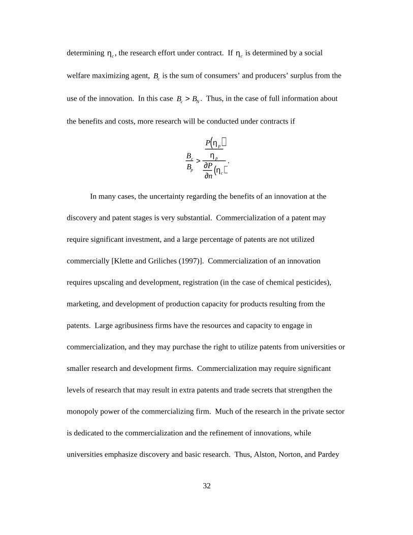
32

determining ηc , the research effort under contract. If ηc is determined by a social

welfare maximizing agent, Bc is the sum of consumers’ and producers’ surplus from the

use of the innovation. In this case Bc > BN . Thus, in the case of full information about

the benefits and costs, more research will be conducted under contracts if

Bc

Bp

>

P ηp( )ηp

∂P∂n

ηc( ).

In many cases, the uncertainty regarding the benefits of an innovation at the

discovery and patent stages is very substantial. Commercialization of a patent may

require significant investment, and a large percentage of patents are not utilized

commercially [Klette and Griliches (1997)]. Commercialization of an innovation

requires upscaling and development, registration (in the case of chemical pesticides),

marketing, and development of production capacity for products resulting from the

patents. Large agribusiness firms have the resources and capacity to engage in

commercialization, and they may purchase the right to utilize patents from universities or

smaller research and development firms. Commercialization may require significant

levels of research that may result in extra patents and trade secrets that strengthen the

monopoly power of the commercializing firm. Much of the research in the private sector

is dedicated to the commercialization and the refinement of innovations, while

universities emphasize discovery and basic research. Thus, Alston, Norton, and Pardey

33

(1995) argue that private-sector and public-sector research spending are not perfect

substitutes. Actually, there may be some complementarity between the two. An increase

in public sector research leads to patentable discoveries, and when private companies

obtain the rights to the patents, they will invest in commercialization research. Private

sector companies have recognized the unique capacity of universities to generate

innovations, and this has resulted in support for university research in exchange for

improved access to obtain rights to the innovations [Rausser (1999)].

Factors beyond the Farm Gate

Over the years, product differentiation in agriculture has increased along with an increase

in the importance of factors beyond the farm gate and within specialized agribusiness.

This evolution is affecting the nature and analysis of agricultural research. Economists

have recently addressed how the vertical market structure of agriculture conditions the

benefits of agricultural research, and also how farm-level innovation may contribute to

changes in the downstream processing sector.

One salient fact about the food-processing sector is that it tends to be

concentrated. The problem of oligopsonistic competition in the food processing sector

has been addressed by Just and Chern (1980), Wann and Sexton (1992), and Hamilton

and Sunding (1997). Two recent papers by Hamilton and Sunding (1998) and Alston,

Sexton, and Zhang (1997) point out that the existence of noncompetitive behavior

34

downstream has important implications for the impacts of farm-level technological

change.

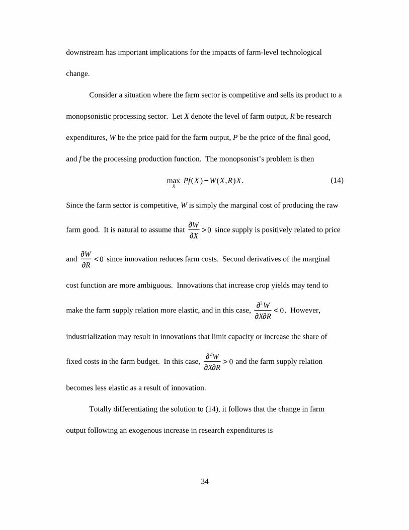
Consider a situation where the farm sector is competitive and sells its product to a

monopsonistic processing sector. Let X denote the level of farm output, R be research

expenditures, W be the price paid for the farm output, P be the price of the final good,

and f be the processing production function. The monopsonist’s problem is then

maxX

Pf(X ) − W(X ,R)X . (14)

Since the farm sector is competitive, W is simply the marginal cost of producing the raw

farm good. It is natural to assume that ∂W

∂X> 0 since supply is positively related to price

and ∂W

∂R< 0 since innovation reduces farm costs. Second derivatives of the marginal

cost function are more ambiguous. Innovations that increase crop yields may tend to

make the farm supply relation more elastic, and in this case, ∂2W

∂X∂R< 0 . However,

industrialization may result in innovations that limit capacity or increase the share of

fixed costs in the farm budget. In this case, ∂2W

∂X∂R> 0 and the farm supply relation

becomes less elastic as a result of innovation.

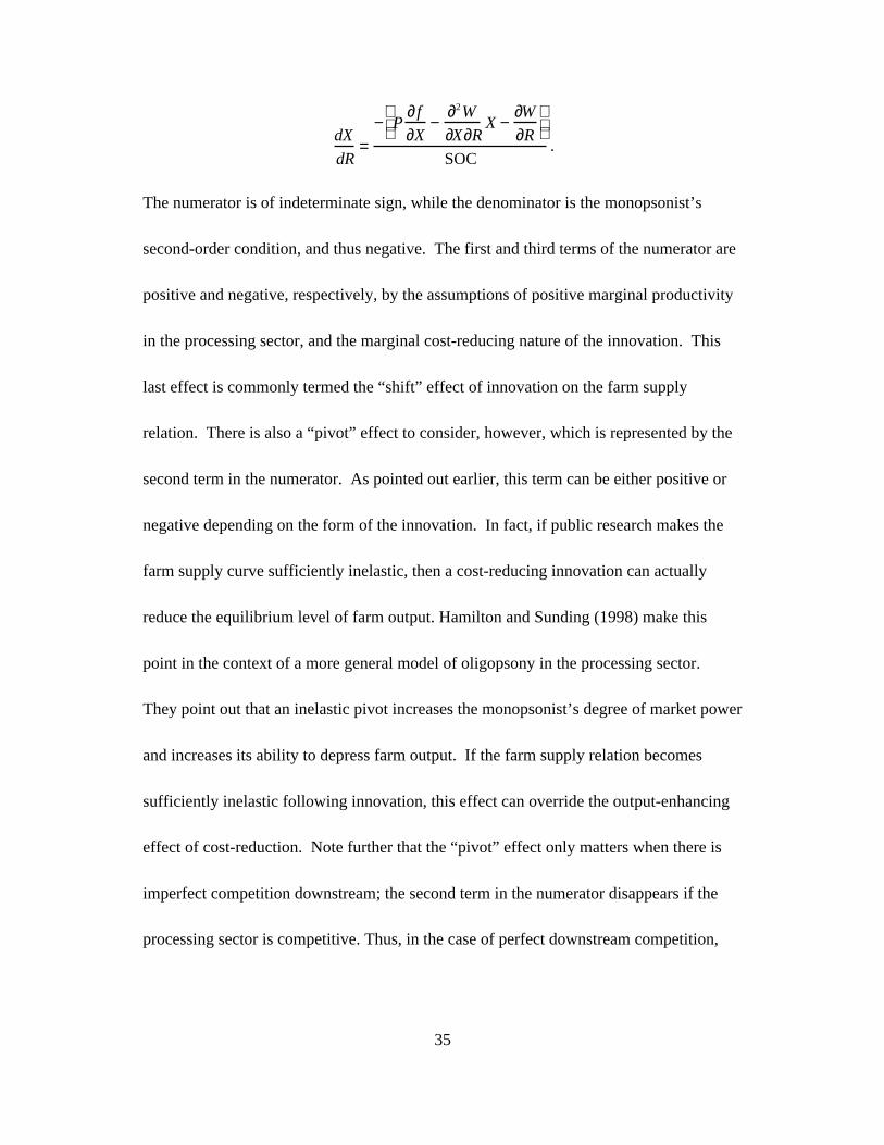
Totally differentiating the solution to (14), it follows that the change in farm

output following an exogenous increase in research expenditures is

35

dX

dR=

− P∂ f

∂X−

∂2W

∂X∂RX −

∂W

∂R

SOC.

The numerator is of indeterminate sign, while the denominator is the monopsonist’s

second-order condition, and thus negative. The first and third terms of the numerator are

positive and negative, respectively, by the assumptions of positive marginal productivity

in the processing sector, and the marginal cost-reducing nature of the innovation. This

last effect is commonly termed the “shift” effect of innovation on the farm supply

relation. There is also a “pivot” effect to consider, however, which is represented by the

second term in the numerator. As pointed out earlier, this term can be either positive or

negative depending on the form of the innovation. In fact, if public research makes the

farm supply curve sufficiently inelastic, then a cost-reducing innovation can actually

reduce the equilibrium level of farm output. Hamilton and Sunding (1998) make this

point in the context of a more general model of oligopsony in the processing sector.

They point out that an inelastic pivot increases the monopsonist’s degree of market power

and increases its ability to depress farm output. If the farm supply relation becomes

sufficiently inelastic following innovation, this effect can override the output-enhancing

effect of cost-reduction. Note further that the “pivot” effect only matters when there is

imperfect competition downstream; the second term in the numerator disappears if the

processing sector is competitive. Thus, in the case of perfect downstream competition,

36

reduction of the marginal cost of farming is a sufficient condition for the level of farm

output to increase.

The total welfare change from farm research is also affected by downstream

market power. In the simple model above, social welfare is given by the following

expression:

SW = P(Z)dZ0

Y ( X ( R))

∫ − W0

X ( R)

∫ (Z , R)dZ , (15)

where P(Z) is the inverse demand function for the final good. The impact of public

research is then

dSW

dR= P

∂f

∂X− W

dX

dR−

∂W

∂RdZ

0

X

∫ .

This expression underscores the importance of downstream market structure. Under

perfect competition, the wedge between the price of the final good and its marginal cost

is zero, and so the first term disappears. In this case, the impact of farm research on

social welfare is determined completely by its impact on the marginal cost of producing

the farm good.8 When the processing sector is imperfectly competitive, however, some

interesting results emerge. Most importantly, if farm output declines following the cost-

reducing innovation (which can only occur if the farm supply relation becomes more

inelastic), then social welfare can actually decrease. This argument was developed in

Hamilton and Sunding (1998), who describe the final outcome of farm-level innovation

8 This point has also been noted recently in Sunding (1996) in the context of environmental regulation.

37

as resulting from two forces: the social welfare improving effect of farm cost reduction

and the welfare effect of changes in market power in the processing industry.

Hamilton and Sunding (1998) show that the common assumption of perfect

competition may seriously bias estimates of the productivity of farm-sector research.

Social returns are most likely to be overestimated when innovation reduces the elasticity

of the farm supply curve, and when competition is assumed in place of actual imperfect

competition. Further, Hamilton and Sunding demonstrate that all of the inverse supply

functions commonly used in the literature preclude the possibility that ∂2W

∂X∂R> 0, and

thus rule out, a priori, the type of effects that result from convergent shifts. More

flexible forms and more consideration of imperfect competition are needed to capture the

full range of possible outcomes.

The continued development of agribusiness is leading to both physical and

intellectual innovation. Feed suppliers, in an effort to expand their market, contributed to

the evolution of large-scale industrialized farming. This is especially true in the poultry

sector. Until the 1950s, separate production of broilers and chickens for eggs were

scarce. The price of chicken meat fluctuated heavily and that limited producers’ entry

into the emerging broiler industry. Feed manufacturers provided broiler production

contracts with fixed prices for chicken meat, which led to vertical integration and modern

industrial methods of poultry production. These firms not only offer output contracts, but

38

they also provide production contracts and contribute to the generation of production

technology. Recently, this same phenomenon has occurred in the swine sector, where

industrialization has reduced the cost of production.

But agribusiness has spurred the development of another set of quality-enhancing

innovations. Again, some of the most important developments have been in the poultry

industry. Tyson Foods and other companies have produced a line of poultry products

where meats are separated according to different categories, cleaned, and ready to be

cooked. The development of these products was based on the recognition of consumers’

willingness to pay to save time in food preparation. In essence, the preparation of poultry

products has shifted labor from the household to the factory where it can be performed

more efficiently.

In addition to enhancing the value of the final product, the poultry agribusiness

giants introduced institutional technological innovations in poultry production [Goodhue

(1997)]. Packing of poultry has shifted to rather large production units that have

contractual agreements with processors/marketers. The individual production units

receive genetic materials and production guidance from the processor/marketer, and their

pay is according to the relative quality. This set of innovations in production and

marketing has helped reduce the relative price of poultry and increase poultry

consumption in the United States and other countries in the last 20 years. Similar

institutional and production innovations have occurred in the production of swine, high-

39

value vegetables, and, to some extent, beef. These innovations are major contributors to

the process of industrialization of agriculture. While benefiting immensely from

technology generated by university research, these changes are the result of private sector

efforts and demonstrate the important contributions of practitioners in developing

technologies and strategies.

II. TECHNOLOGY ADOPTION

Adoption and Diffusion

There is often a significant interval between the time an innovation is developed and

available in the market, and the time it is widely used by producers. Adoption and

diffusion are the processes governing the utilization of innovations. Studies of adoption

behavior emphasize factors that affect if and when a particular individual will begin using

an innovation. Measures of adoption may indicate both the timing and extent of new

technology utilization by individuals. Adoption behavior may be depicted by more than

one variable. It may be depicted by a discrete choice, whether or not to utilize an

innovation, or by a continuous variable that indicates to what extent a divisible

innovation is used. For example, one measure of the adoption of a high-yield seed

variety by a farmer is a discrete variable denoting if this variety is being used by a farmer

40

at a certain time; another measure is what percent of the farmer’s land is planted with this

variety.

Diffusion can be interpreted as aggregate adoption. Diffusion studies depict an

innovation that penetrates its potential market. As with adoption, there may be several

indicators of diffusion of a specific technology. For example, one measure of diffusion

may be the percentage of the farming population that adopts new innovations. Another is

the land share in total land on which innovations can be utilized. These two indicators of

diffusion may well convey a different picture. In developing countries, 25 percent of

farmers may own or use a tractor on their land. Yet, on large farms, tractors will be used

on about 90 percent of the land. While it is helpful to use the term “adoption” in

depicting individual behavior towards a new innovation and “diffusion” in depicting

aggregate behavior, in cases of divisible technology, some economists tend to distinguish

between intra-firm and inter-firm diffusion. For example, this distinction is especially

useful in multi-plant or multi-field operations. Intra-firm studies may investigate the

percentage of a farmer’s land where drip irrigation is used, while inter-firm studies of

diffusion will look at the percentage of land devoted to cotton that is irrigated with drip

systems.

41

The S-Shaped Diffusion Curve

Studies of adoption and diffusion behaviors were undertaken initially by rural

sociologists. Rogers (1962) conducted studies on the diffusion of hybrid corn in Iowa

and compared diffusion rates of different counties. He and other rural sociologists found

that in most counties diffusion was an S-shaped function of time. Many of the studies of

rural sociologists emphasized the importance of distance in adoption and diffusion

behavior. They found that regions that were farther away from a focal point (e.g., major

cities in the state) had a lower diffusion rate in most time periods. Thus, there was

emphasis on diffusion as a geographic phenomenon.

Statistical studies of diffusion have estimated equations of the form

Yt = K 1 + e− a + bt( )[ ]−1, (16)

where Yt is diffusion at time t (percentage of land for farmers adopting an innovation), K

is the long-run upper limit of diffusion, a reflects diffusion at the start of the estimation

period, and b is a measure of the pace of diffusion.

With an S-shaped diffusion curve, it is useful to recognize that there is an initial

period with a relatively low adoption rate but with a high rate of change in adoption.

Figure 3 shows this as a period of introduction of a technology. Following is a takeoff

period when the innovation penetrates the potential market to a large extent during a short

period of time. During the initial and takeoff periods, the marginal rate of diffusion

42

actually increases, and the diffusion curve is a convex function of time. The takeoff

period is followed by a period of saturation where diffusion rates are slow, marginal

diffusion declines, and the diffusion reaches a peak. For most innovations, there will also

be a period of decline where the innovation is replaced by a new one (Figure 3).

Insert Figure 3

Griliches’ (1957) seminal study on adoption of hybrid corn in Iowa’s different

counties augmented the parameters in (16) with information on rates of profitability, size

of farms in different counties, and other factors. The study found that all three

parameters of diffusion function (K, a, and b) are largely affected by profitability and

other economic variables. In particular, when ∆π denotes the percent differential in

probability between the modern and traditional technology, Griliches (1957) found that

∂a ∂∆π , ∂K ∂∆π , and ∂b ∂∆π are all positive. Griliches’ work (1957, 1958) spawned

a large body of empirical studies [Feder, Just, and Zilberman (1985)]. They confirmed

his basic finding that profitability gains positively affect the diffusion process. The use

of S-shaped diffusion curves, especially after Griliches (1957) introduced his economic

version, has become widespread in several areas. S-shaped diffusion curves have been

used widely in marketing to depict diffusion patterns of many products, for example,

consumer durables. Diffusion studies have been an important component of the literature

on economic development and have been used to quantitatively analyze the processes

through which modern practices penetrate markets and replace traditional ones.

43

Diffusion as a Process of Imitation

The empirical literature spawned by Griliches (1957, 1958) established stylized facts, and

a parallel body of theoretical studies emerged with the goal of explaining its major

findings. Formal models used to depict the dynamics of epidemics have been applied by

Mansfield (1963) and others to derive the logistic diffusion formula. Mansfield viewed

diffusion as a process of imitation wherein contacts with others led to the spread of

technology. He considered the case of an industry with identical producers, and for this

industry the equation of motion of diffusion is

∂Yt

∂ t= bYt 1 −

Yt

K

. (17)

Equation (17) states that the marginal diffusion at time t (∂Y / ∂t , the actual

adoption occurring at t) is proportional to the product of diffusion level Yt and the

unutilized diffusion potential 1 − Yt / K( ) at time t. The proportional coefficient b

depends on profitability, firm size, etc. Marginal diffusion is very small at the early

stages when Yt → 0 and as diffusion reaches its limit, Yt → K . It has an inflection point

when it switches from an early time period of increasing marginal diffusion

∂ 2Yt / ∂ t 2> 0( ) to a late time period of decreasing marginal diffusion ∂ 2Y / ∂ t2< 0( ). For

an innovation that will be fully adopted in the long run K = 1( ) , ∂Yt / ∂ t = bYt 1 − Yt( ) , the

inflection point occurs when the innovation is adopted by 50 percent of producers.

Empirical studies found that the inflection point occurs earlier than the simple dynamic

44

model in (17) suggests. Lehvall and Wahlbin (1973) and others expanded the modeling

of the technology diffusion processes by incorporating various factors of learning and by

separating firms that are internal learners (innovators) from those that are external

learners (imitators). This body of literature provides a very sound foundation for

estimation of empirical time-series data on aggregate adoption levels. However, it does

not rely on an explicit understanding of decision making by individual firms. This

criticism led to the emergence of an alternative model of adoption and diffusion, the

threshold model.

The Threshold Model

Threshold models of technology diffusion assume that producers are heterogeneous and

pursue maximizing or satisfying behavior. Suppose that the source of heterogeneity is

farm size. Let L denote farm size and g(L) be the density of farm size. Thus, g(L)∆L is

the number of farms between L − ∆L / 2 and L + ∆L / 2 . The total number of farms is

then N = g(L)dL0

∞

∫ , and the total acreage is L = Lg(L)dL0

∞

∫ .

Suppose that the industry pursued a traditional technology that generated π0 units

of profit per acre. The profit per acre of the modern technology at time t is denoted by

π1(t) and the profit differential per acre is ∆πt . It is assumed that an industry operates

under full certainty, and adoption of modern technology requires a fixed cost that varies

45

over time and at time t is equal to Ft . Under these assumptions, at time t there will be a

cutoff farm size, LtC = Ft ∆π t , upon which adoption occurs. One measure of diffusion at

time t is thus

Yt1 =

g L( )dLLt

C

∞

∫N

, (18)

which is the share of farms adopting at time t. Another measure of diffusion of time t is

Yt2 =

Lg L( )dLLt

C

∞

∫L

, (19)

which is the share of total acres adopting the modern technology at time t.

The diffusion process occurs as the fixed cost of the modern technology declines

over time ∂Ft / ∂ t < 0( ) or the variable cost differential between the two technologies

increases over time ∂∆πt / ∂ t > 0( ). The price of the fixed cost per farm may decrease

over time because the new technology is embodied in new indivisible equipment or

because it requires an up-front investment in learning. “Learning by doing” may reduce

fixed costs through knowledge accumulation. The profit differential often will increase

over time because of “learning by using.” Namely, farmers will get more yield and save

cost with more experience in the use of the new technology.

46

The shape of the diffusion curve depends on the dynamics of farm size and the

shape of farm size distribution. Differentiation of (18) obtains marginal diffusion under

the first definition

∂Yt1

∂ t= −

g LtC( )

N

∂LtC

∂ t. (20)

Marginal diffusion at time t is equal to the percentage of farms adopting technology at

this time. It is expressed as ∂ LtC / ∂ t times the density of the farm size distribution at

LtCg Lt

C( ) .

The dynamics of diffusion associated with the threshold model are illustrated in

Figure 4. Farm size distribution is assumed to be unimodal. When the new innovation is

introduced, only farms with a size greater than L0C will adopt. The critical size declines

over time and this change triggers more adoption. The marginal adoption between the

first and second year is equal to the area abL2CL1

C . Figure 4 assumes that the marginal

decline in LtC is constant because of the density function’s unimodality. Marginal

diffusion increases during the initial period (from 0 to 1 t s ), and then it declines, thus

leading to an S-shaped diffusion curve. It is plausible that farm size distribution (and the

distribution of other sources of heterogeneity) will be unimodal and that combined with a

continuous decline of LtC will lead to S-shaped behavior.9

9 To have an S-shaped behavior, f

2Yt

1 ft 2 > 0 for an initial period with t t< $ and f2Yt

1 ft 2 < 0 for

t t> $ . Differentiation of (20) yields

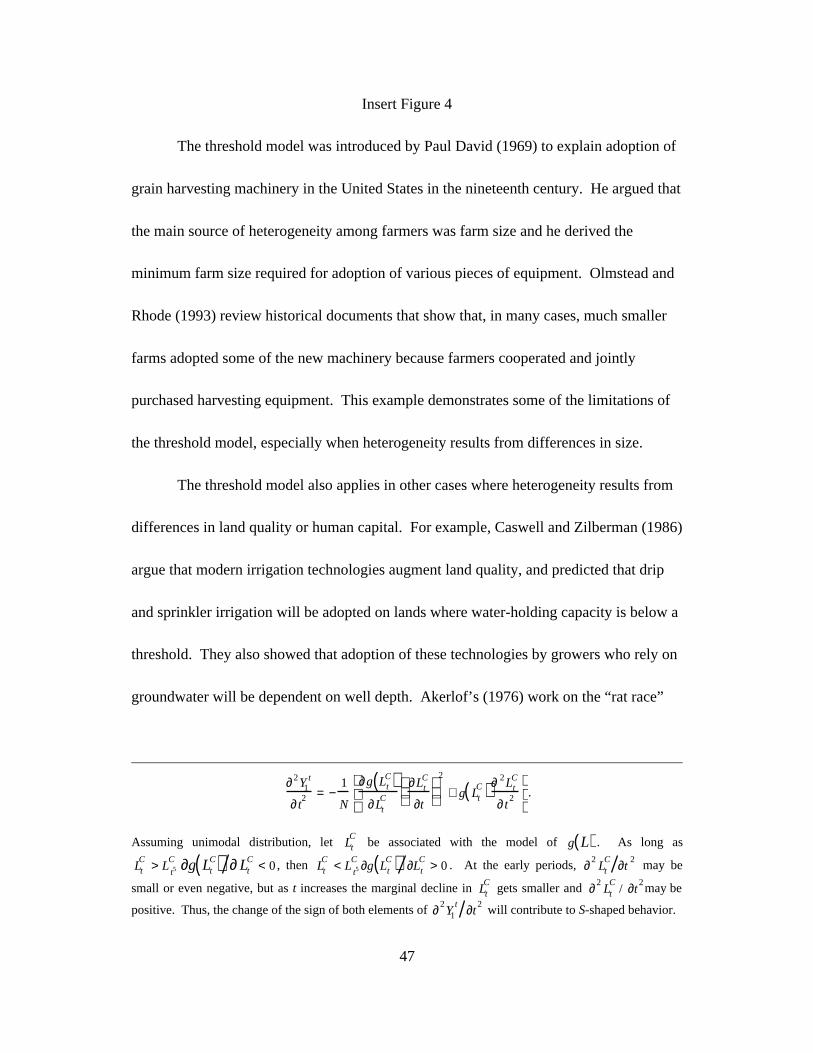
47

Insert Figure 4

The threshold model was introduced by Paul David (1969) to explain adoption of

grain harvesting machinery in the United States in the nineteenth century. He argued that

the main source of heterogeneity among farmers was farm size and he derived the

minimum farm size required for adoption of various pieces of equipment. Olmstead and

Rhode (1993) review historical documents that show that, in many cases, much smaller

farms adopted some of the new machinery because farmers cooperated and jointly

purchased harvesting equipment. This example demonstrates some of the limitations of

the threshold model, especially when heterogeneity results from differences in size.

The threshold model also applies in other cases where heterogeneity results from

differences in land quality or human capital. For example, Caswell and Zilberman (1986)

argue that modern irrigation technologies augment land quality, and predicted that drip

and sprinkler irrigation will be adopted on lands where water-holding capacity is below a

threshold. They also showed that adoption of these technologies by growers who rely on

groundwater will be dependent on well depth. Akerlof’s (1976) work on the “rat race”

∂2Y1

t

∂ t2 = −

1

N

∂g LtC( )

∂LtC

∂LtC

∂t

2

+ g LtC( )∂ 2Lt

C

∂ t2

.

Assuming unimodal distribution, let LtC

be associated with the model of g L( ) . As long as

LtC > L

t5C ∂g Lt

C( ) ∂ LtC < 0 , then Lt

C < Lt5C ∂g Lt

C( ) ∂LtC > 0 . At the early periods, ∂2

LtC ∂t

2 may be

small or even negative, but as t increases the marginal decline in LtC gets smaller and ∂2

LtC

/ ∂t2may be

positive. Thus, the change of the sign of both elements of ∂2Y1

t ∂t2 will contribute to S-shaped behavior.

48

suggests that differences in human capital establish thresholds and result in differences in

the adoption of different technologies and practices.

The threshold models shifted empirical emphasis from studies of diffusion to

studies of the adoption behavior of individual farmers and a search for sources of

heterogeneity. Two empirical approaches have been emphasized in the analysis of

monthly cross-sectional data on technological choices and other choices of parameters

and characteristics of individual firms. In the more popular approach, the dependent

variables denote whether or not certain technologies are used by a farm product or unit at

a certain period, and econometric techniques like logit or probit are used to explain

discrete technology choices. The dependent variable for the second approach denotes the

duration of technologies used by farms. (They answer the question, How many years ago

did you adopt a specific technology?) Also, limited variable techniques are used to

explain the technology data. Qualitatively, McWilliams and Zilberman (1996) found that

the two approaches will provide similar answers, but analysis of duration data will enable

a fuller depiction of the dynamics of diffusion.

Geographic Considerations

Much of the social science literature on innovation emphasizes the role of distance and

geography in technology adoption [Rogers (1962)]. Producers in locations farther away

49

from a regional center are likely to adopt technologies later. This pattern is consistent

with the findings of threshold models because initial learning and the establishment of a

new technology may entail significant travel and transport costs, and these costs increase

with distance.

Diamond’s (1999) book on the evolution of human societies emphasizes the role

of geography in the adoption of agricultural technologies. China and the Fertile Crescent

have been source regions for some of the major crops and animals that have been

domesticated by humans. Diamond argues that the use of domestic animals spread

quickly throughout Asia and laid the foundation for the growth of the Euro-Asian

civilizations that became dominant because most of these societies were approximately at

the same geographic latitude, and there were many alternative routes that enabled

movement of people across regions. The diffusion of crop and animal systems in Africa

and the Americas was more problematic because population movement occurred along

longitudinal routes (south to north) and thus, technologies required substantial

adjustments to different climatic conditions in different latitudes. Diamond argues that

there were other geographic barriers to the diffusion of agricultural technologies. For

example, the slow evolution of agricultural societies in Australia and Papua New Guinea

is explained by their distance from other societies, which prevented diffusion of practices

from elsewhere.

50

Geography sets two barriers to adoption: climatic variability and distance.

Investment in infrastructure to reduce transportation costs (e.g., roads and telephone

lines) is likely to accelerate adoption. One reason for the faster rate of technological

adoption in the United States is the emergence of a national media and the drastic

reduction in the cost of access that resulted from the establishment of railroads, the

interstate highway system, and rural electrification.

Distance is a major obstacle for adoption of technologies in developing countries.

The impediment posed by distance is likely to decline with the spread of wireless

communication technologies. It is a greater challenge to adopt technologies across

different latitudes and varying ecological conditions. The establishment of international

research centers that develop production and crop systems for specific conditions is one

way to overcome this problem.

Risk Considerations

The adoption of a new technology may expand the amount of risk associated with

farming. Operators are uncertain about the properties and performance of a new

technology, and these uncertainties interact with the random factors affecting agriculture.

The number of risks associated with new technologies gives rise to several modeling

approaches, each emphasizing aspects of the problem that are important for different

types of innovations. In particular, some models will be appropriate for divisible

51

technologies and others for lumpy ones, and some will explicitly emphasize dynamic

aspects while others will be static in nature.

Much of the agricultural adoption literature was developed to explain adoption

patterns of high-yield seed varieties (HYV), many of which were introduced as part of

the “green revolution.” Empirical studies established that these technologies were not

fully adopted by farmers in the sense that farmers allocated only part of their land to

HYV while continuing to allocate land to traditional technologies. Roumasset (1976) and

others argued that risk considerations were crucial in explaining these diversifications,

while having higher expected yield also tended to increase risk.

A useful approach to model choices associated with adoption of HYV is to use a

static expected utility portfolio model to solve a discrete problem (whether or not to adopt

the new technology at all); adoption can also be modeled as a continuous optimization

problem in which optimal land shares devoted to new technologies and variable inputs

are chosen [see Just and Zilberman (1988); Feder and O’Mara (1981)].

To present these choices formally, consider a farmer with L acres of land, which

can be allocated among two technologies. Let i be a technology variable, where i = 0

indicates the traditional technology, and i = 1 the modern one. Let the indicator variable

be δ = 0 when the modern technology is adopted (even if not adopted on all the land),

and δ1 = 0 when the modern technology is not adopted. When δ = 1, L0 denotes land

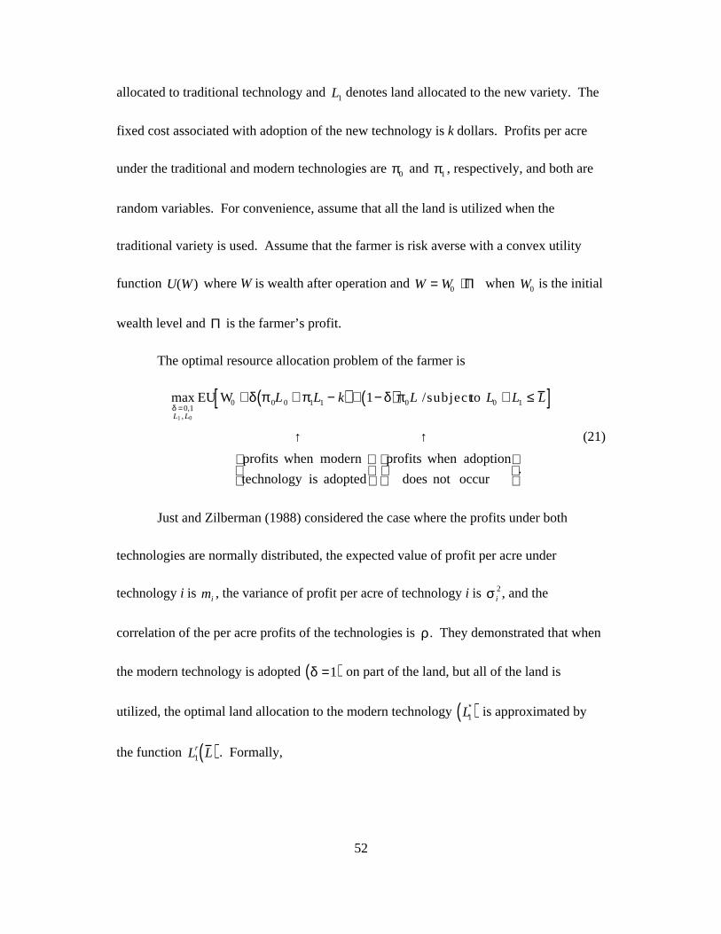
52

allocated to traditional technology and L1 denotes land allocated to the new variety. The

fixed cost associated with adoption of the new technology is k dollars. Profits per acre

under the traditional and modern technologies are π0 and π1 , respectively, and both are

random variables. For convenience, assume that all the land is utilized when the

traditional variety is used. Assume that the farmer is risk averse with a convex utility

function U(W) where W is wealth after operation and W = W0 + Π when W0 is the initial

wealth level and Π is the farmer’s profit.

The optimal resource allocation problem of the farmer is

maxδ = 0,1L1 , L0

EU W0 + δ π 0L0 + π1L1 − k( ) + 1− δ( )π0L /subjectto L0 + L1 ≤ L [ ]

↑ ↑profits when modern

technology is adopted

profits when adoption

does not occur

.

(21)

Just and Zilberman (1988) considered the case where the profits under both

technologies are normally distributed, the expected value of profit per acre under

technology i is mi , the variance of profit per acre of technology i is σ i2 , and the

correlation of the per acre profits of the technologies is ρ . They demonstrated that when

the modern technology is adopted δ =1( ) on part of the land, but all of the land is

utilized, the optimal land allocation to the modern technology L1∗( ) is approximated by

the function L1r L ( ) . Formally,

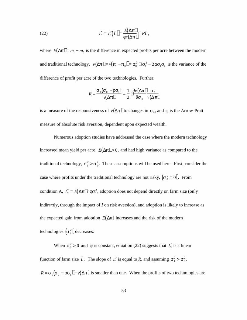
53

(22) L1* = L1

r L ( ) =E ∆π( )φr ∆π( ) + RL ,

where E ∆π( ) = m1 − m0 is the difference in expected profits per acre between the modern

and traditional technology. v ∆π( ) = v π1 −π 0( ) = σ02 + σ1

2 − 2ρσ1σ0 is the variance of the

difference of profit per acre of the two technologies. Further,

R =σ 0 σ0 − ρσ1( )

v ∆π( ) =1

2⋅∂v ∆π( )

∂σ 0

σ 0

v ∆π( )

is a measure of the responsiveness of v ∆π( ) to changes in σ0, and φ is the Arrow-Pratt

measure of absolute risk aversion, dependent upon expected wealth.

Numerous adoption studies have addressed the case where the modern technology

increased mean yield per acre, E ∆π( ) > 0 , and had high variance as compared to the

traditional technology, σ12 > σ 0

2 . These assumptions will be used here. First, consider the

case where profits under the traditional technology are not risky, σ 02 = 0( ) . From

condition A, L1* = E ∆π( ) / φσ1

2 , adoption does not depend directly on farm size (only

indirectly, through the impact of I on risk aversion), and adoption is likely to increase as

the expected gain from adoption E ∆π( ) increases and the risk of the modern

technologies σ12( ) decreases.

When σ02 > 0 and φ is constant, equation (22) suggests that L1

r is a linear

function of farm size L . The slope of L1r is equal to R, and assuming σ1

2 > σ02 ,

R = σ 0 σ0 − ρσ1( ) − v ∆π( ) is smaller than one. When the profits of two technologies are

54

highly correlated, ρ > σ 0 / σ1, R < 0 , dL1R / dL < 0 , and acreage of the modern

technology declines with farm size. This occurs because the marginal increase with

acreage (variance of profits) is larger than the marginal increase of expected profits that

slow the growth or even reduce (when ρ > σ 0 / σ ) the acreage of the modern and more

risky technology of larger farms.

Assume now that absolute risk aversion is a function of farm size (a proxy of

expected wealth) denoted by φ L( ) . In this case, Just and Zilberman showed that the

marginal effect of increase on the area of the modern technology is

dL1r

dL = η

L1r

L + r −η( )R ,

where η = −′ φ L

φ is the elasticity of absolute risk aversion and is assumed to be between 0

(η = 0 implies constant absolute risk aversion) and 1 (η = 1 implies constant relative risk

aversion coefficient, φ L( ) ⋅ L = constant). In this more general case, L1r may be a

nonlinear function of L and may have a negative slope in cases of high correlation and

small η .

Optimal land allocation to the modern technology, L1∗ , is constrained to be

between 0 and L . Thus, it may be different than L1r defined in (22). In cases with small

η (φ does not change much with L ), the increase in risk (variance of profits) with size is

much greater than the increase in expected profit with size. When L is close to zero,

55

L1R > L and thus where farm size is below a critical level, L b ,10 the modern technology

should be fully adopted if it is optimal. From (22) the adoption of the modern technology

is optimal if it pays for the extra investment it entails. Thus, farms below another critical

size, L a , cannot pay for the modern technology and do not adopt it.

Figure 5 depicts some plausible relations between L1* and L . The segment 0abcd

depicts the behavior of L1* when R > 0 and L b > L a . If L b > L a and R < 0, L1

* is depicted

by 0abce. If L a > L b , and R > 0 , L1* is depicted by 0gh and if L a > L b and R < 0 , L1

* is

depicted by 0gle. In the last two cases, there is no full adoption of the modern

technology.

Feder, Just, and Zilberman (1985) report the results of several studies that show

that when adoption occurs, the full share of modern technologies declines with farm size

among adopters. These findings are consistent with all the scenarios in Figure 5.

Insert Figure 5

Mechanisms to Address Performance and Fit Risk

Adopters of new technologies, especially if embodied in high capital costs that entail

significant irreversible investment, face uncertainty with respect to the performance of

10 At L = L

b, L

1r

L ( )b = L b

.

56

the product, its reliability, and appropriateness of their operation. When a farmer buys a

piece of machinery—be it a combine, harvester, seeder, or cultivator—and it has a

breakdown or major malfunction, it may cost a farmer much of his revenues.

Conceptually, one may think about several solutions to address some risk, including

insurance. The prevailing approach to address such risk is to form a product-backup

system. To address the financial risks that are associated with the repair cost of a broken

or malfunctioning product, especially in the early life of the product, manufacturers

introduced mechanisms such as warranties and established dealerships equipped to repair

breakdowns. Thus, the combination of a warranty agreement and a well-functioning

technical support system significantly reduce the amount of reliability risk associated

with new products.

Significant elements of agribusinesses, such as mechanic shops, are devoted to the

repair and maintenance of new capital equipment. The availability and quality of

performance of this support will determine the risk farmers face in adoption decisions

and, thus, their ability to carry risk. One of the main advantages of large farming

operations is their in-house capacity to handle repairs, breakdowns, and maintenance of

equipment. That makes them less dependent on local dealers and repair shops, and

reduces their risk of having to purchase (in many cases) new products.

The value of the capacity to address problems of product equipment failure

swiftly and efficiently is intensified by timing considerations. In many regions,

57

harvesting seasons are short. Leaving a wheat crop unharvested for an extra day or two

may expose it to damage due to rain, hail, or pests, thereby decreasing its yield. Market

prices of perishable fruits and vegetables are significantly dependent on the timing of

harvest; a one-week delay in harvesting early season fruits or vegetables for shipping can

reduce prices by factors of 30 to 40 percent [Parker and Zilberman (1993)]. This timing

consideration increases the value of a well-functioning product system. It may provide

an explanation for the maintenance of excess capacity to harvest or conduct other vital

activities. Of course, the extent to which farmers maintain excess capacity depends on

how well the product support system functions. The agricultural community may

establish customs and other social and institutional arrangements for mutual help in a

crisis situation associated with a breakdown of equipment.

Adoption of new technology entails risk with respect to its appropriateness to the

farm and its performance. Results of prior testing by manufacturers represent

performance and conditions that may not be exactly similar to those of farmers. New

technologies may also require special skills and training. Institutional arrangements to

reduce the risk associated with the adoption of new technologies have been introduced.

They include product information and demonstration such as educational materials in

various media formats as well as hands-on demonstrations. The farmer may go to a

showroom to see farm machinery in operation or the equipment may be loaned to the

farmers for a supervised and/or unsupervised trial period. For new seed varieties,

58

manufacturers will send farmers samples of seeds for examination. Many farms will

plant small trial plots.

When university researchers are the providers of new seeds, extension plays a

major role in demonstration. In the case of new seed varieties and equipment developed

by the private sector, extension plays an important role in demonstrating efficacy in local

conditions as well as making objective judgments on manufacturers’ claims regarding

new products.

In addition to various types of extension, the reduction of risk associated with

performance and the appropriateness of new technologies is addressed by arrangements

such as money-back guarantees. With money-back guarantees, the farmer is given the

option to return the product. In this case, obviously the price of the product includes

some payment for this option [Heiman, Zhao, and Zilberman (1998)]. However, the

money-back guarantee agreement allows farmers longer periods of experimentation with

new products. Generally money-back guarantees are not complete and a fraction of the

original cost is not returned.

Sometimes renting is used as a mechanism to reduce the risk associated with

investment in new products. For example, when sprinkler irrigation was introduced in

California, the main distributor of sprinklers in the state was a company called Rain for

Rent. This company rented sprinkler equipment to farmers. Over time, the practice of

renting sprinkler equipment became much less common and more new sprinkler

59

equipment was purchased. In some cases, farmers use custom services for an initial trial

with new technologies, and invest in the equipment only when they feel more secure and

certain about its properties.

Many of the marketing strategies, including warranties, money-back guarantees,

and demonstrations that are part of businesses throughout the economy, were introduced

by agricultural firms including John Deere and International Harvesting. Currently,

hundreds of millions of dollars are spent on promotion and education in the use of new

products. Unfortunately, not much research has been conducted to understand this aspect

of agricultural and technological change in agriculture. It seems, however, that a large

body of empirical evidence regarding geographic concentration of new technologies and

geographic patterns of technology adoption may be linked to considerations of marketing

and product support efforts. New technologies are more likely to be adopted earlier near

market centers where dealers and product supports are easily available. Agricultural

industries and certain types of technologies may be clustered in certain regions,

especially in the earlier life of a new technology, and these regions will generally be

located in areas that have technical support and expertise associated with the maintenance

and development of the technologies. It seems that considerations of marketing and

geographic locations are two areas where more research should be done.

60

Dynamic Considerations

The outcome of technology adoption is affected by dynamic processes that result in

changes in prices of capital goods and input, learning by producers and users of capital

goods, etc. Some of these processes have random components and significant uncertainty

over time. Some of these dynamic considerations have been introduced to recent

microlevel models of adoption behavior.

Optimal Timing of Technology Adoption

The earlier discussion on threshold models recognized that timing of adoption may vary

across production units reflecting differences in size, human capital, land quality, etc.

The above analysis suggests that, at each moment, decision-makers select technologies

with the best-expected net benefits (or expected net present values adjusted by risk).

Thus, when a new technology is available decision-makers continuously evaluate

whether or not to adopt; when the discounted expected benefits of adoption are greater

than the cost, the technology will be adopted. This approach may lead to suboptimal

outcomes because decision-makers do not consider the possibility of delaying the

technology choice to take advantage of favorable dynamic processes or to enable further

learning. These deficiencies have been corrected in recent models.

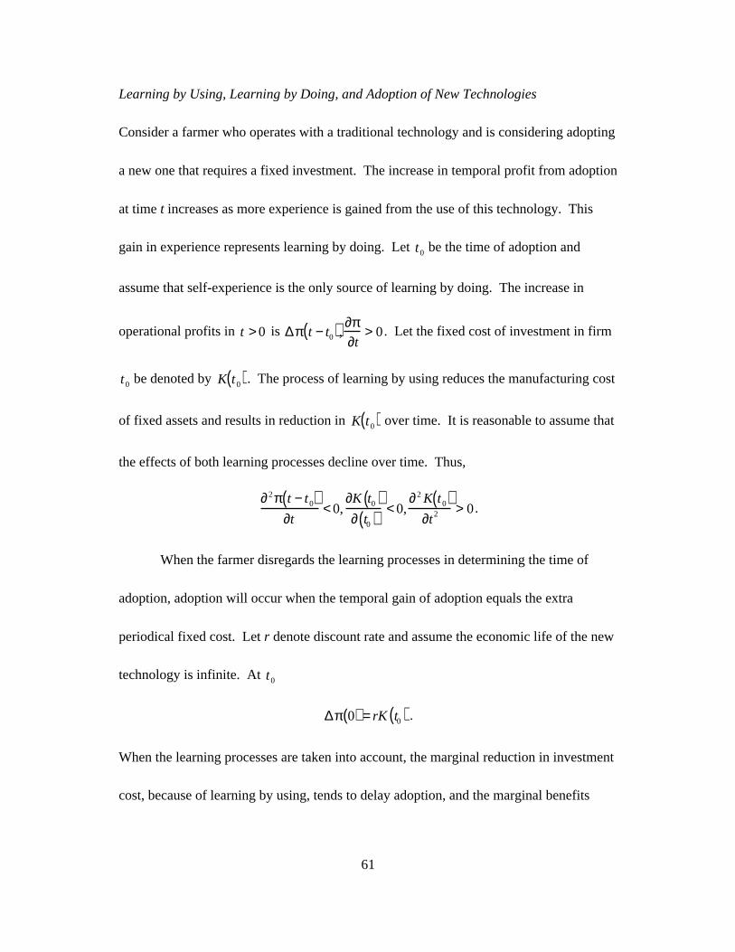
61

Learning by Using, Learning by Doing, and Adoption of New Technologies

Consider a farmer who operates with a traditional technology and is considering adopting

a new one that requires a fixed investment. The increase in temporal profit from adoption

at time t increases as more experience is gained from the use of this technology. This

gain in experience represents learning by doing. Let t0 be the time of adoption and

assume that self-experience is the only source of learning by doing. The increase in

operational profits in t > 0 is ∆π t − t0( ), ∂π∂t

> 0 . Let the fixed cost of investment in firm

t0 be denoted by K t0( ). The process of learning by using reduces the manufacturing cost

of fixed assets and results in reduction in K t0( ) over time. It is reasonable to assume that

the effects of both learning processes decline over time. Thus,

∂2π t − t0( )∂t

< 0,∂K t0( )∂ t0( ) < 0,

∂2 K t0( )∂t2 > 0 .

When the farmer disregards the learning processes in determining the time of

adoption, adoption will occur when the temporal gain of adoption equals the extra

periodical fixed cost. Let r denote discount rate and assume the economic life of the new

technology is infinite. At t0

∆π 0( ) = rK t0( ) .

When the learning processes are taken into account, the marginal reduction in investment

cost, because of learning by using, tends to delay adoption, and the marginal benefits

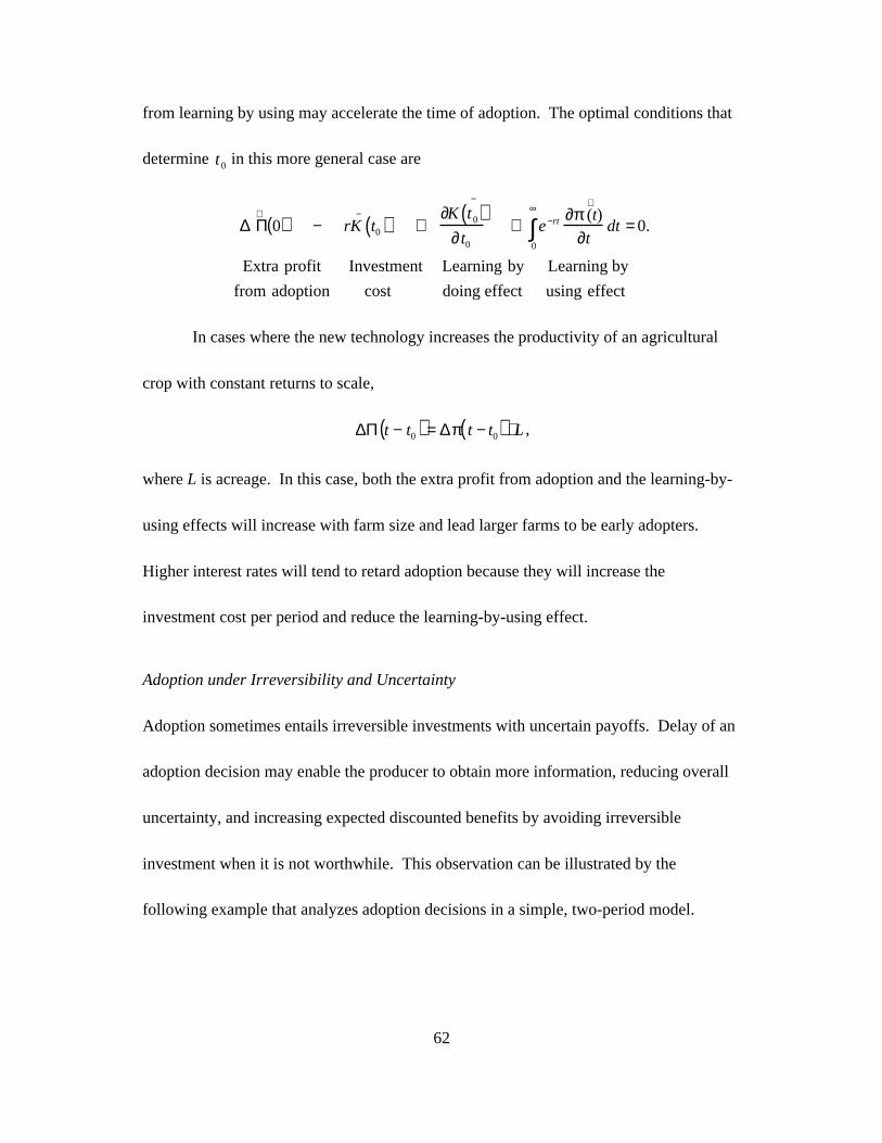
62

from learning by using may accelerate the time of adoption. The optimal conditions that

determine t0 in this more general case are

∆ Π+

0( ) − rK−

t0( ) +∂K t0( )

−

∂ t0

+ e−rt

0

∞

∫∂π (t)

+

∂tdt = 0.

Extra profit Investment Learning by Learning by

from adoption cost doing effect using effect

In cases where the new technology increases the productivity of an agricultural

crop with constant returns to scale,

∆Π t − t0( ) = ∆π t − t0( ) ⋅ L ,

where L is acreage. In this case, both the extra profit from adoption and the learning-by-

using effects will increase with farm size and lead larger farms to be early adopters.

Higher interest rates will tend to retard adoption because they will increase the

investment cost per period and reduce the learning-by-using effect.

Adoption under Irreversibility and Uncertainty

Adoption sometimes entails irreversible investments with uncertain payoffs. Delay of an

adoption decision may enable the producer to obtain more information, reducing overall

uncertainty, and increasing expected discounted benefits by avoiding irreversible

investment when it is not worthwhile. This observation can be illustrated by the

following example that analyzes adoption decisions in a simple, two-period model.

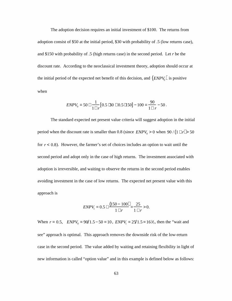
63

The adoption decision requires an initial investment of $100. The returns from

adoption consist of $50 at the initial period, $30 with probability of .5 (low returns case),

and $150 with probability of .5 (high returns case) in the second period. Let r be the

discount rate. According to the neoclassical investment theory, adoption should occur at

the initial period of the expected net benefit of this decision, and ENPV0( ) is positive

when

ENPV0 = 50 +1

1+ r0.5 ⋅30 + 0.5 ⋅150[ ] − 100 =

90

1+ r− 50 .

The standard expected net present value criteria will suggest adoption in the initial

period when the discount rate is smaller than 0.8 (since ENPV0 > 0 when 90 / 1 + r( ) > 50

for r < 0.8). However, the farmer’s set of choices includes an option to wait until the

second period and adopt only in the case of high returns. The investment associated with

adoption is irreversible, and waiting to observe the returns in the second period enables

avoiding investment in the case of low returns. The expected net present value with this

approach is

ENPV1 = 0.5 +150 − 100( )

1 + r=

25

1 + r> 0.

When r = 0.5, ENPV0 = 90 1.5 − 50 = 10 , ENPV1 = 25 1.5 = 1623 , then the “wait and

see” approach is optimal. This approach removes the downside risk of the low-return

case in the second period. The value added by waiting and retaining flexibility in light of

new information is called “option value” and in this example is defined below as follows:

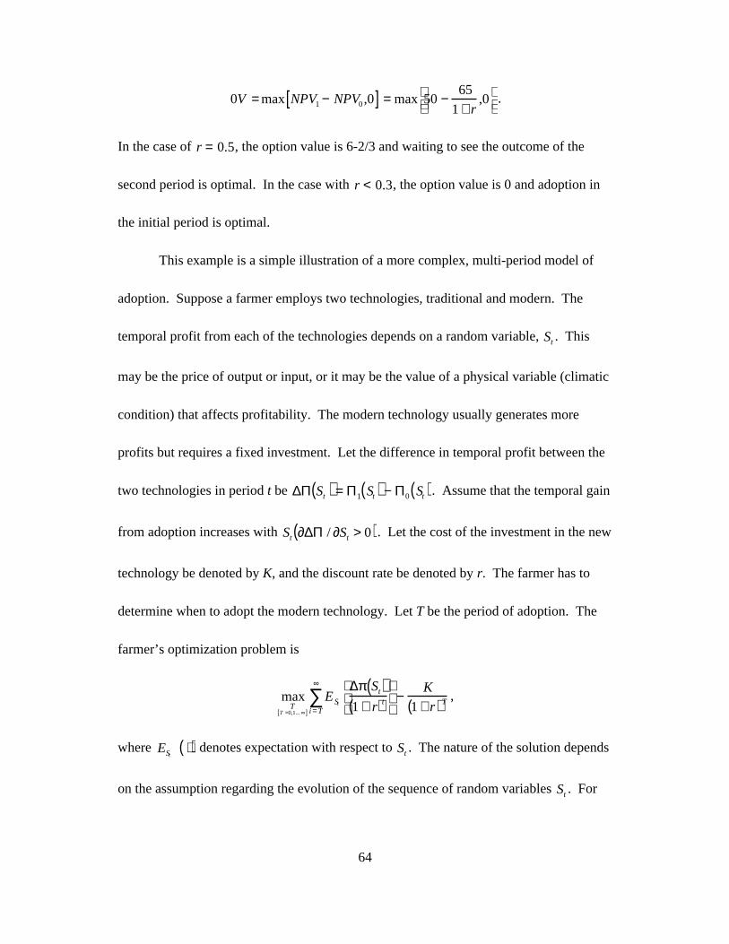
64

0V = max NPV1 − NPV0 ,0[ ] = max 50 −65

1 + r,0

.

In the case of r = 0.5, the option value is 6-2/3 and waiting to see the outcome of the

second period is optimal. In the case with r < 0.3, the option value is 0 and adoption in

the initial period is optimal.

This example is a simple illustration of a more complex, multi-period model of

adoption. Suppose a farmer employs two technologies, traditional and modern. The

temporal profit from each of the technologies depends on a random variable, St . This

may be the price of output or input, or it may be the value of a physical variable (climatic

condition) that affects profitability. The modern technology usually generates more

profits but requires a fixed investment. Let the difference in temporal profit between the

two technologies in period t be ∆Π St( ) = Π1 St( ) − Π0 St( ). Assume that the temporal gain

from adoption increases with St ∂∆Π / ∂St > 0( ). Let the cost of the investment in the new

technology be denoted by K, and the discount rate be denoted by r. The farmer has to

determine when to adopt the modern technology. Let T be the period of adoption. The

farmer’s optimization problem is

maxT

T =0,1... ∞[ ]

ESt

i = T

∞

∑ ∆π St( )1 + r( )t

−

K

1 + r( )T ,

where ESt ⋅( ) denotes expectation with respect to St . The nature of the solution depends

on the assumption regarding the evolution of the sequence of random variables St . For

65

example, suppose St = St −1 + εt where all the ε t ’s are independently and identically

distributed random variables whose means are zero. (If they are normally distributed, St

is generated by a “random walk” process.) This approach has been very successful in the

analysis of options in finance, and Dixit and Pindyck (1994) and McDonald and Siegel

(1986) applied it to the analysis of capital investments. They viewed investments with

unrestricted timing as “real options” since the decision about when to undertake an

investment is equivalent to the decision about when to exercise an option. McDonald and

Siegel (1986) considered a continuous time model to determine the time of investment.

They assumed that the S evolves according to a Wiener process (which is a differential

continuous version of the process described above) and used the Ito calculus to obtain

formulas to determine the threshold for adoption S . Their analysis suggests that the

threshold level of S increases as the variance of the temporal random variable ε t

increases.

Their framework was applied by Hasset and Metcalf (1992) to assess adoption of

energy conservation in the residential sectors. Thurow, Boggess, and Moss (1997)

applied the real option approach to assess how uncertainty and irreversibility

considerations will affect adoption of free-stall dairy housing, a technology that increases

productivity and reduces pollution. The source of uncertainty in their case is future

environmental regulation. Using simulation techniques, they showed that when

66

investment is optimal under the real option approach, expected annual returns are more

than twice the expected annual returns associated with adoption under the traditional net

present value approach. Thus, the real value approach may lead to a significant delay in

adoption of the free-stall housing and occurs when pollution regulations are very stiff.

Olmstead (1998) applied the real value approach to assess adoption of modern

irrigation technology when water prices and availability are uncertain. Her simulation

suggests that the water price leading to adoption under the real option approach is 133

percent higher than the price that triggers adoption under the standard expected net

present value approach. In her simulation, the average delay in adoption associated with

the real option approach is longer than 12 years.

There have been significant studies of adoption of irrigation technologies and,

while adoption levels seemed to respond significantly to economic incentives, adoption

did not occur in many of the circumstances when it was deemed to be optimal using the

expected present value criteria. Much of the adoption occurs during drought periods

when water prices escalate drastically [Zilberman et al. (1994)]. The option value

approach provides a good explanation of the prevalence of adoption during crisis

situations.

The analysis of adoption behavior using “real options” models holds much

promise and is likely to be expanded. In many cases, not all the adoption investment is

“sunk cost.” Some of it can be recovered. For example, capital goods may be resold, and

67

added human capital may increase earning opportunities. The delay caused by adoption

costs and uncertainties will likely be shorter if these costs are more recoverable, and

institutions that reduce irreversibilities (rental of capital equipment, money-back

guarantee agreements) are apt to increase and accelerate adoption.

The real option approach provides new insight and is very elegant, but it does not

capture important aspects of the dynamics of adoption. It assumes that decision makers

know the distribution of random events that determine profitability when it is more likely

that a learning process is going on throughout the adoption process, and adopters adjust

their probability estimates as they go along. Furthermore, while adoption requires a fixed

initial investment, it also may entail incremental investments, especially when the

intensity of use of a new technology changes over time. Thus, a more complete dynamic

framework for analyzing adoption should address issues of timing, learning, and

sequential investment. Some scholars [Chavas (1993)] have introduced models that

incorporate these features, but this research direction requires more conceptual and

empirical work.

The Cochrane Treadmill

A key issue in the economics of innovation and adoption is to understand the impact of

technology change on prices and, in particular, the well being of the farm population over

time. When a supply-increasing innovation is adopted to a significant degree, it will lead

68

to reduction in output prices, especially in agricultural commodities with low elasticity of

demand. When it comes to adoption of a new technology, Cochrane (1979) divided the

farming population into three subgroups—early adopters, followers, and laggards. The

early adopters may be a small fraction of the population, in which case the impact of their

adoption decision on aggregate supply and, thus, output prices is relatively small.

Therefore, these individuals stand to profit from the innovation.

The followers are the large share of the farm sector who tend to adopt during the

take-off stage of the innovation. Their adoption choice will eventually tend to reduce

prices, which reduces profits as well. This group of adopters may gain or lose as a result

of innovation.

Finally, the laggards (the third group) are the farmers who either adopt at the lag

stage of the adoption process or do not adopt at all. These individuals may lose from

technological change. If they do not adopt, they reduce the same quantity as before, at

low prices; and if they adopt, the significant price effect may sweep the gain associated

with higher yields. Thus, Cochrane argues that farmers, on the whole, are not likely to

gain from the introduction of innovation in agriculture, except for a small group of early

adopters. Introduction of new technology may lead to structural change and worsen the

lot of some of the small farms. The real gainers from technological change and

innovation in agriculture are likely to be consumers, who pay less for their food bill.

69

Kislev and Schori-Bachrach (1973) developed conceptual and empirical models

based on Cochrane’s analysis using data from Israel. They show that small subgroups of

farmers are the early innovators who adopt the new technologies. When there is a wave

of new technologies, these individuals, who have a higher education and other indicators

of human capital, will consistently be able to take advantage of technology change and

profit. The rest of the farming population does not do as well from technological change.

The Cochrane results are modified in situations where agricultural commodities

face perfectly elastic demand, for example, when adopting industry export goods from a

small country. In this case, the impact of increased profitability associated with the

introduction of a new technology will lead to an increase in land rents which may occur

some time after the innovation was introduced. Thus, the early adopters, even if they are

farm operators, may be able to make an above-normal profit as a result of their adoption

decision, but most of the followers will not gain much from the adoption decision

because their higher revenues will be reduced by an increase in rent. Laggards and

nonadopters may lose because the higher rent may reduce their profits. Again, you have

a situation where landowners will be gainers from the innovations and not the farmers.

Thus, this extension of Cochrane’s model reaches the same conclusion--that farmers do

not benefit from technological change as much as other agents in the population.

Cochrane’s modeling framework was used to argue that, in spite of the high

technological change that occurs in agriculture and its dynamic nature, farmers may not

70

be better off and actually some of them may be worse off from innovations. That may

justify the “farm problem” that occurred in much of the twentieth century where the well

being of farmers became worse relative to other sectors of the population. Cochrane’s

basic framework was not introduced formally. Zilberman (1985) introduced the

dynamics of the threshold model of adoption that identified conditions under which the

quasi-rents of farmers decline over time. His model did not take into account the changes

in structure that may be associated with innovation agriculture. When innovations are

embodied in technology packages that are both yield-increasing (high-yield varieties) and

labor-saving (tractors and other machinery), and agricultural demand is inelastic, then

technological change will reduce quasi rent per acre and make operations in the farm

sector less appealing to a large segment of the population. Thus the early adopters are

likely to accumulate more of the land, increasing their farm size. Over time, structural

change will result in a relatively small farm sector, and earnings per farm may actually

increase as farms become much bigger. Gardner’s (1988) findings show that, in relative

terms, the farm population is now as well off or even better off than the nonfarm

population, especially in the United States. His findings are consistent with the process

of technological change that led to the accumulation of resources by small subgroups of

the farm population while the rest migrated to the urban sector where earnings were

better. But in addition to the gains from technological change, the adopters may also

71

have benefited from a commodity program that slowed the decline in prices as well as the

processes of globalization that may demand more elasticity over time.

A more formal and complete understanding of the distribution and price

implications of technological change over time is a challenge for further research on the

economics of technology adoption. Stoneman and Ireland (1983) argue that firms

producing the components of new technology recognize the dynamics of adoption; they

design their production and establish technology component prices accordingly, taking

advantage of the monopolistic power. Thus there is a clear linkage between the

economics of innovation and adoption that should be investigated further. An

understanding of these links is essential for the design of better patent policy and public

research strategies.

Institutional Constraints to Innovation

While agricultural industries tend to be competitive, the perfectly competitive model does

not necessarily apply since farmers may face a significant number of institutional

constraints and policies which affect their behavior significantly and result in outcomes

that are different from those predicted by the perfectly competitive model. This

institutional constraint may be especially important in the area of technological change

and adoption. Some of the most important constraints relate to credit as well as tenure

relationships, as addressed below. Note that institutional constraints may affect the

72

patterns of adoption of new technologies, but on the other hand, the introduction of new

technologies may affect the institutional structure and operation of agricultural industries.

We will concentrate on the first problem but will address both.

Credit

Asymmetric information between lenders and borrowers, and the uncertain conditions in

agriculture and financial markets have led to imperfections in the credit market, most

notably credit constraints that affect adoption behavior [Hoff, Braverman, and Stiglitz

(1993)]. In many cases, farmers use some of their own equity to finance at least part of

their investments. In other cases, assets such as land or the crop itself are used as

collateral for financing a new technology. The exact formulation of the credit constraint

faced by farmers is quite tricky, but it is not unreasonable to approximate as a linear

function of acreage. The reason is that, in many cases, land is the major asset of a

farming operation.

Just and Zilberman (1983) introduced a credit constraint in their static model of

adoption under uncertainty. They assume that investment in the new technology is equal

to k +αL1 when α is investment per acre in the modern technology. The constraint on

credit per acre is m dollars. Thus, the farm credit constraint is mL ≥ k + αL1. If m < α1,

there will be full adoption. However, if m > α , the credit constraint will not bind for

larger farms. Figure 6 depicts some plausible outcomes for the second case. Consider a

73

case where R > 0 and L a < L b . Without the credit constraints, optimal allocation of land

to the modern technology, as a function of farm size, is depicted by 0abcd in Figure 6.

There may be several scenarios under the credit constraints.

Insert Figure 6

In terms of Figure 6, when credit is a binding constraint, L1 < −k

α+

m

αL . Small

farms (with sizes in the range 0a) will be non-adopters. Somewhat larger farms, in the

range bh, will be credit-constrained partial adopters. Even larger farms (in the range hc)

will specialize in the new technology, and farms of the largest size (corresponding to cd)

will be risk diversifiers when m is smaller. Policies to remove credit constraints will be

beneficial, especially to smaller farmers, and will enable some to adopt and others to

extend their intensity of adoption.

The credit constraints per acre may be affected by the lender’s perception of the

profitability of agriculture (and farmland prices that reflect the profitability). Initial

subsidization of credit early in the diffusion process that will enhance adoption will

provide evidence that may change (improve in the case of a valuable technology) the

lender’s perception of the profitability of the industry and the modern technology, and

lead to a relaxation of credit constraints. It will thus facilitate further adoption.

The interest rate and other financial charges may be differentiated according to

size. A bank may perceive smaller farms to be more risky, they may need to compensate

74

for the fixed cost of loan processing, etc.11 If the price of credit is higher for smaller

farms, that extra hurdle will reduce the minimal farm size that is required for new

technology adoption and will slow adoption by smaller sized farms. Thus, advantageous

credit conditions may be another reason larger farms adopt new technologies earlier. The

reduction of institutions such as the Grameen Bank in Bangladesh and organizations such

as the Bank of America in the United States, which in the beginning of the century

facilitated loans to smaller operations, may be a crucial element in accelerating the

process of technological change in improving adoption.

The financial crisis of the 1980s has led to a realization of the significance of risk

associated with emphasizing collateral considerations in loan generation. The value of

assets such as land is highly correlated to the profitability of agriculture and, in periods of

crises and bankruptcies, land will be less valuable as collateral. That will lead to an

increased emphasis on the “ability to pay” as criteria for loan generation. Thus, farmers

need to provide sufficient guarantees about the profitability of their investment and their

future ability to repay a loan. This may put investment in new technologies at a

disadvantage because many of them do not have a sufficient track record that will assure

banks of their economic viability. Banks may lack the personnel that are able to correctly

assess new technologies and their economic value [Agricultural Issues Center (1994)].

11 There is significant evidence in the development literature that smaller operators face a higher interestcost.

75

One approach to overcome this obstacle is by credit subsidies for a new

technology, which may be appropriate in situations when investments generate positive

externalities. However, an alternative and more prevalent solution is the provision of

finance or a loan guarantee by the input manufacturer that leads to a reduction of the

financial constraints on farmers. Furthermore, it reduces the fixed cost of adoption since

it reduces the cost of searching for a loan. (One of the major implications of restricted

availability of credit is the higher cost of finance, even for people who eventually obtain

the credit.) Indeed, some of the major automobile and heavy equipment companies have

their own subsidiaries or contractual arrangements that provide financing for new

purchases of equipment, and seed companies often play an important role in the provision

of credit. In many cases farmers may obtain loans for credit provisions through

cooperatives or government policies (see chapter on credit).

Tenure

There is a distinct separation between ownership and the operation of agricultural land

throughout the world. About 50 percent of the farmland in the United States is operated

by individuals who do not own the land, and the financial arrangements between owners

and operators vary. In the development literature, there is a significant emphasis on the

importance of tenure systems on technology adoption. Most of the literature takes tenure

as given and assesses its impact on adoption of technologies. However, this impact

76

depends on the arrangements as well as the nature of the technology. Furthermore, as we

will argue later, the introduction of new technologies may result in new tenure

relationships.

The simplest relationships are land rent contracts where operators pay a fixed rent

to landowners. Several factors will determine how these contracts affect adoption

behavior. In the case of short-term contracts, when operators are not secure in

maintaining the same land for a long time, the likelihood that they will adopt a

technology that requires investment in the physical infrastructure and improvement of the

land is very low. In these cases, rental relationships may be a significant deterrent for the

adoption of innovations. On the other hand, the fixed-rate rent will not be a major

deterrent of adoption if the innovation does not require a significant modification of the

physical infrastructure, or if it augments or is dependent upon the human or physical

capital of the operator. For example, an operator may purchase a tractor to reduce the

cost of his operation. The necessary condition for adoption in this case is that the

operator rent a sufficient amount of land every year in order to recapture and repay the

investment. Actually, in some cases, the existence of a well-functioning land rental

market may accelerate adoption of technologies that require a significant scale of

operation. In fact, some farmers may augment the land utilized by them by renting land

from others, thus enabling them to adopt large equipment. This was the situation, for

example, in California when the cotton harvester was introduced. Therefore, it is useful

77

to distinguish between large operators who use rental agreements to increase the acreage

under their control (the rental agreements may facilitate adoption) and small operators

without land of their own. For these operators, due to the credit constraints, lack of land

may be a deterrent for adoption, even for technologies that do not improve the land and

related assets.

Complementary Inputs and Infrastructure

The introduction of new technologies may increase demand for complementary inputs

and when the supply of these inputs is restricted, adoption will be constrained. High-

yield “green revolution” varieties require increased water and fertilizer use. McGuirk

and Mundlak’s (1991) analysis of the adoption of high-yield varieties in the Punjab

showed that adoption was constrained by the availability of water and fertilizer. Private

investment in the drilling of wells, and private and public investment in the establishment

of fertilizer production and supply facilities removed these constraints and contributed to

the diffusion of modern wheat and rice varieties in the Punjab. The adoption of high-

yield maize varieties in the Punjab was much lower than wheat and rice, mostly because

of disease problems. Adoption rates in maize might have been higher if complementary

disease-control technologies were available.

Some of the complementary input constraints are eased or eliminated with the

appropriate infrastructure. Effective research and extension programs may devise

78

solutions to pest problems thus enabling the adoption of vulnerable varieties. Some of

the modeling and analysis of diffusion [Mahajan and Peterson (1985)] suggest that the

diffusion rates in regions that are farther from commercial centers are lower. To some

extent this reflects barriers for professional support and more limited and costly access to

complementary inputs. Improvement in transportation infrastructure may thus be useful

for enhancing adoption.

Adoption and Farm Policy

Agriculture in developing and developed countries has been subject to government

interventions that, in turn, affect technological change. Generally speaking, agricultural

policies in developed countries aim to raise and stabilize agricultural incomes and, in

some cases, to curtail supplies, while agricultural outputs have been taxed in developing

nations. In both cases agricultural inputs have tended to be subsidized.

In recent years, agriculture has been subject to new environmental policies that

control and affect the use of certain inputs that may cause pollution. The following is a

discussion of the impacts of different policies on technological change.

Price Supports

Just, Rausser, and Zilberman (1986) and Just et al. (1988) developed a framework,

relying on the model presented in equation (21), to analyze the impact of agricultural

79

policies on technology adoption for farmers operating under uncertainty. They analyze

various policies by tracing their impacts on price distributions of inputs and outputs as

well as constraints (i.e., credit) on adoption. Price supports increase the mean of prices

received by farmers and reduce their variability by setting lower price bounds. When the

new technology has a yield-increasing effect (for example, high-yield variety), and if it is

also perceived to have higher risk, price-support policies tend to increase its relative

profitability, which leads to an increase in both the extent and intensity of adoption.

McGuirk and Mundlak (1991) argue that the introduction of guaranteed markets for

Punjabi food grain production by the government procurement policy (which was in

essence a price support policy) enhanced the adoption of high-yield wheat and rice

varieties in this region.

The mechanism through which price supports impact the adoption behavior of

farms of different sizes varies. Smaller farms may increase their adoption because of

price supports (their impact on credit) and the reduction in the minimum size required to

justify adoption. Larger farms that may be risk diversifiers will increase the share of

modern technologies on their land because of the mean effect and the reduction in risk.

Price supports may also enhance adoption of mechanical innovations when they increase

the relative profitability of operations with a new technology and thus reduce the size

threshold required for adoption. Price supports may enhance adoption also through their

80

impact on credit. When the ability to obtain credit depends on expected incomes, price

supports will increase adoption when credit is constrained.

Combined Output Price Supports and Land Diversion Policies

In the United States as well as in some European countries, the subsidization of prices has

been accompanied by a conditional reduction in acreage. The higher and most secure

prices on at least part of the land provide incentives for farmers to adopt yield-increasing

varieties. On these lands, they raise the value of property and expected income, which

increases their capacity to obtain credit that may enhance the adoption of all types of

technologies.

Specific elements of the support program vary over time. In recent years, the base

for support has not been the actual yield, but the average base yield that is dependent on

the average past performance of either the farmer or the region. The acreage that

provides the base for entitlement to the benefits of a diversion program also depends on

past performance. According to the specifics of a program, farmers might expand their

yield or acreage in order to expand their entitlements in the future. Thus, adoption of

high yielding technologies, or technologies that may be especially beneficial with

marginal land, is more likely to occur with price supports/diversion policies.12 The

historical record that provides a base for future program entitlements may, on the other

12 The work of Zilberman (1984) provides a rigorous argument on the impact of programs such asdeficiency payments and diversion policies on the expansion of acreage and supply.

81

hand, provide disincentives to adopt new crops or to introduce nonprogram crops to

certain areas and thus reduce the flexibility of farming. The Freedom to Farm Act in the

United States makes entitlements that are independent of most farming activities,

including choice of crop. However, even under this bill, land that is entitled to income

support is somewhat restricted in its choice of crops, and that may retard the adoption and

introduction of new crops to some of the major field crop regions of the United States.

Cochrane (1979) argued that the commodity programs in the United States played

a major role in the adoption of mechanical and chemical innovations by reducing risk and

increasing profitability per acre. The commodity programs as well as the increases in

demand and prices during and after World War II led to modernization and structural

change in U.S. agriculture. De Gorter and Fisher (1993) used a dynamic model to show

that the combination of price supports and land diversion led to intensification of farming

in the United States. Lichtenberg’s (1989) work demonstrates the importance of

economic incentives for the adoption of center-pivot irrigation in Nebraska and other

Midwestern states, and suggests that expansion of the irrigated land base in these states

benefited from the support programs of the 1970s and 1980s.

Output Taxation

Taxation of agricultural outputs, prevalent especially in developing countries, has a

disastrous effect on technological change. It reduces the incentive to adopt yield-

82

increasing technologies, increases the scale of operation that justifies financing purchases

of new equipment, and depresses the price of agricultural land, thus reducing the ability

to borrow. Furthermore, with lower prices, there are incentives to apply intensively

modern inputs, which are associated in many cases with the adoption of modern, high-

yield varieties in developing countries. The low growth of Argentinian agriculture

between 1940 and 1973 is a result of output taxation and other policies that reduced

relative prices to agriculture and slowed investments and technological change in this

sector [Cavallo and Mundlak (1982)].

Trade Liberalization and Macroeconomic Policies

The adoption of innovations is likely to be significantly influenced by policies that affect

the general economy. This may include trade and exchange rate policies as well as

macroeconomic and credit policies. Macroeconomic policies that lead to high interest

rates may reduce adoption because investment in new technologies is more costly.

Adoption of mechanical innovations may suffer more significantly with high interest

rates, while farmers may switch to technologies that are labor-intensive.

Changes in international trade regimes will affect various regions differently

according to their relative advantage. The opening of markets in the United States led to

the introduction of high-value varieties in different communities in Central America

[Carletto, de Janvry, and Sadoulet (1996)]. This change in cropping was combined with

83

the establishment of a new infrastructure and the construction of packinghouses and

transportation facilities. Thus, when a change in trade rules seems permanent, it may

lead to a complete overhaul of the infrastructure, and that may enable adoption of new

crops and modernization.

Favorable pricing because of trade barriers enables growers in Europe, Japan, and

some parts of the United States to adopt yield-increasing varieties, to invest and develop

greenhouse technologies, and to expand the capacity of different technologies, including

irrigated agriculture, in situations that would not have warranted it under free trade. The

growth and investment in the agricultural sector in both Argentina and Chile suffered

during periods when international trade was constrained, and benefited from trade

liberalization [Coeymans and Mundlak (1993); Cavallo and Mundlak (1982)].

Environmental Policies

A wide array of environmental regulations affects technologies available for agriculture.

Pesticide bans provide a strong incentive for the development of alternatives at the

manufacturer level and for the adoption of alternative strategies including nonchemical

treatment, biological control, etc. On the other hand, the lack of availability of chemicals

may retard adoption of high-yield varieties or new crops that are susceptible to a

particular pest, especially in cases where nonchemical alternatives are not very effective.

The elimination of DBCP (with its unique capacity to treat soil-borne diseases) in the

84

mid-1980s in California led, on the one hand, to the abandonment of some grape acreage

and a switch to other crops. At the same time, it enhanced the adoption of drip irrigation

that enabled applications of alternatives in other areas.

Input Subsidies

There is a wide body of literature [Caswell (1991)] that shows that subsidized water

pricing tends to retard the adoption of modern irrigation technologies. However,

subsidized input led to the adoption of high-yield varieties and “green revolution”

technologies in countries like India. They also increased profitability and thus have an

indirect positive impact on adoption through credit effects. Similarly, subsidization of

pesticides and fertilizers led to the adoption of high-yield varieties and chemical-

intensive technologies in developing and developed countries alike, which is also likely

to result in problems of environmental pollution since the environmental side effects of

agriculture are often the result of excessive residues. Alternatively, elimination of

subsidies and especially taxation of chemical inputs may lead to adoption of more precise

application technologies that will reduce residues and actually may increase yield

[Khanna and Zilberman (1997)].

Conditional Entitlements of Environmental Programs

Governments have recognized that they can use entitlements to support programs

conditional on certain patterns of behavior. Therefore, in recent years there have been

85

attempts to link entitlements to income supports, policies, and other subsidization to

certain patterns of environmental behavior. A program like the Environmental Quality

Incentives Program (EQIP) in the United States attempts to induce farmers to adopt

practices such as low-tillage and soil testing, and to reduce the application of chemicals

in exchange for entitlements for some support. In some cases, the benefits of such a

program are short-lived and farmers may quit using modern practices once the program

benefits disappear. On the other hand, especially when it comes to new, untested

technologies, elements of learning-by-doing and experience may improve the profitability

of those technologies that have some environmental benefits so that farmers recognize

their economic advantages. Thus, the adoption of such technologies may persist in the

long run.

III. FUTURE DIRECTIONS

Research on agricultural technology evolves from the technology and the institutions

associated with it. At present, agriculture is undergoing a technological revolution as

evidenced by the introduction of biotechnology and precision technology. We are also

witnessing related processes of industrialization, product differentiation, and increased

vertical integration in agriculture [Zilberman, Sunding, and Khanna (1997)]. These

changes raise new issues and introduce new challenges. Several significant changes have

86

been observed thus far from the emergence of biotechnology [Zilberman, Yarkin, and

Heiman (1998)].

With many past technologies, university research identified some of the basic

concepts while most of the innovations were done in industries. However, with

biotechnology, universities are the source of numerous new discoveries, and technology

transfer from universities to industries has triggered the creation of leading products and

companies. The unwillingness of private firms to develop university innovations without

exclusive rights motivated the establishment of offices of technology transfer that

identified buyers who would share the rights to develop university innovations. Each

arrangement provides new sources of funding to universities since royalties are divided

among universities, researchers, and departments. Thus far, income from technology

transfer revenues has paid less than 5 percent of university research budgets. However,

in some areas (biology and medicine) it made a difference. Most of the royalties were

associated with fewer than 10 innovations [Parker, Zilberman, and Castillo (1998)],

reinforcing our existing knowledge that benefits to research tend to concentrate on a

small number of critical innovations. Established companies were not willing to buy the

rights to develop some of the most radical, yet important, university innovations and

biotechnology. Thus, offices of technology transfer, working with venture capitalists,

helped to establish new upstart companies, some of which became leading biotechnology

firms (e.g., Genentech, Chiron and Amgen). As these companies grew and became

87

successful, some of the major multinationals bought a majority of shares in these

companies. Thus, most of the activities in biotechnology have been in medical

biotechnology. However, 1996 was the breakthrough year for agricultural biotechnology

as millions of acres were planted with pest-resistant varieties of cotton and soybeans. In

agricultural biotechnology, we see again the importance of small startups from the

collaborations between university researchers and venture capitalists. Most of the

startups in agricultural biotechnology have been acquired by giants like Monsanto and

DuPont.

The evolution of biotechnology suggests that the university is becoming a major

player in industrial development, and it affects the structure and competitiveness of

industries. University researchers working with venture capitalists generate new avenues

of product development. Sometimes they may force some of the giant companies to

change their product development strategy, and may even give up some of their

monopolistic power. Other forms of contractual relationships between university

researchers and industries are being established. For example, industries support certain

lines of research for an exclusive option to purchase the rights for technology.

Furthermore, some researchers suddenly find themselves wearing another hat, that of a

partner in a technology company, and that may affect the way universities run their

patterns of payments and support for researchers. Given these new realities, there is a

need for both empirical and conceptual research on innovations and the relationships

88

between public and private research. We need to better understand the existing

arrangements of royalties, sharing of royalties within the university, the relationship

between publications and patents, and the effect of university research and industrial

structure, etc.

With computers, biotechnology, and other new technologies, most of the value is

now embodied in specific knowledge. The Cohen-Boyer patent once generated the

largest revenues to universities. In this case, companies paid for the right to use a process

for genetic manipulation. The key to biotechnology is the process of innovation (that

specifies how to conduct specific manipulation) and product innovation (that specifies

what type of outcomes can be controlled by which genes). New genetic engineering

products will be produced by combining certain procedures and items of knowledge that

are protected by certain patent rights. In principle, the developers of new products should

pay the royalties to whoever owns the patents. Thus the markets for rights to different

types of knowledge will emerge.

A new research agenda is suggested to address the economics of intellectual

property rights. In particular, it should address pricing rules for different types of

intellectual property rights and the design of biotechnology products given the price

structures for different processes and product innovations. An important area of

understanding is the pricing of international property rights within complex international

89

systems where protection of intellectual property rights is not always feasible and where

there are significant disparities in income.

The research in intellectual property rights will also have implications on the

issues of biodiversity and compensation for developing countries for genetic materials

that are embodied in their natural resources. Other related issues include the incentives

for and integration of research to develop basic foods; the alleviation of starvation in the

poorest countries; how new emerging industrial orders in agriculture and biotechnology

can provide appropriate technologies to these countries; defining the role of international

research institutes and other public entities (e.g., the United Nations and global

organizations) in conducting research aimed at the poorest countries; and what type of

payment arrangement should exist between research units focused on developing

countries and commercial firms in the more developed nations.

Materials and chemicals that were previously produced by chemical procedures

may be produced through modified biological organisms. First, biotechnology in

agriculture will produce alternative forms of pest control and pest-resistant varieties but,

over time, they will produce higher quality food products and new products such as

pharmaceuticals and fine chemicals [see Zilberman, Sunding, and Khanna (1997)]. With

biotechnology the value added of seeds will increase to include some of the rent that was

accrued to chemicals. Pesticide manufacturers already have become major players in

biotechnology and are taking over seed companies in order to obtain a channel to market

90

their products. Often the owners of the rights to patents try to capture some of the rent

through contracting; thus, biotechnology will provide both the incentives to enhance

contractual arrangements and vertical integration in agriculture. Some of the recent

mergers and acquisitions in agricultural biotechnology can be explained by attempts to

obtain rights to intellectual property and access to markets [Rausser, Scotchmer, and

Simon (1999)]. Finally, biotechnology causes firms with agricultural characteristics (for

example, dairies, livestock operations, and even field crop operations) to produce

products in areas that are not traditionally agricultural (pharmaceutical, oils, coloring).

As the borderline between agriculture and industry becomes fuzzier, new models replace

the competitive models as the major paradigm to assess agriculture.

The new product lines and the new types of industrial organization that may occur

with biotechnology will raise environmental concerns and management issues.

Biotechnology, thus far, has had a good track record, but it could have a negative

potential. The design of the regulatory framework will significantly affect the structure

of biotechnology industries and their impact. A more restrictive registration process, for

example, may lead to a more concentrated biotechnology. Thus, it will become a

research and policy challenge to modify the registration process and to balance the risks

and benefits associated with biotechnology through monitoring over time. The optimal

design of intellectual property rights agreements in biotechnology will become another

issue of major concern. Patent rights that are too broad will lead to concentration in

91

industries. It may stymie competition but may encourage a small number of firms to

invest heavily in new products. Biotechnology patent protections that are too narrow

may prevent significant investment in a costly research line.

Over the last 30 or 40 years, precision technologies have evolved that adjust input

use to variation over space and time and reduce residues. The use of precision

technologies is still in its infancy. The development of computer and satellite technology

suggests a new, vast potential, but it has had limited use thus far. However, new products

are continuously being introduced, and some types of precision technologies will play a

major role in the future of agriculture. One challenge in improving precision technology

will be to develop the software and management tools that will take advantage of new

information. That will present a significant challenge to researchers in farm

management. Other issues involve the development of institutions that take advantage of

network externalities associated with knowledge and that accumulate and distribute

information that is pertinent to farm management. The pricing of knowledge will also

become a major issue of research within the context of precision farming.

Another important issue associated with precision farming is the potential for

improving environmental quality. The adoption of precision farming may be induced by

environmental regulation. The link between environmental regulation, research,

development, and the adoption of new products needs to become clearer and provide

insight to improve institutions and incentives. Most of the research on technology and

92

innovation thus far has been done within regional bounds, but one of the main challenges

of the future is to analyze issues of research and development within an international

context. We need to better understand issues of technology transfer and intellectual

property rights within nations. In some cases we need to better understand the

mechanisms of collaboration between nations to address either global problems or to take

advantage of increases in returns to scale. International food research centers and some

existing binational research and development arrangements have become very

prominent.13 These types of arrangements may become more important in the future and

should be further investigated. Furthermore, the relationship between the private and the

public sectors in research and development should be viewed in a global context. A

multinational corporation may change the research activities and infrastructure between

nations in response to changes in economic conditions, and the activities of such private

organizations depend both on national and international public sector policies.

International aspects of research and development are especially important in light

of trade agreements such as GATT and NAFTA, and there is very little knowledge on

how international trade agreements affect research and development. However, this type

of knowledge is crucial because R&D is becoming a key element in the evolution of

agricultural industries. An important issue to address, of course, is the development of

13 For evaluation of the Binational Agricultural Research Development (BARD) fund between Israel andthe United States, see Just et al. (1988).

93

research infrastructure on global problems, for example, private global climate change.

Thus far, this research has been conducted by individual nations without much

coordination of finance, finding, and direction. As we recognize our interdependence and

the importance of issues such as global management of natural resources, fisheries, and

biodiversity, we need to determine what type of mechanism we should use to enhance

efficiency and research in knowledge development on a global basis?

In addition to an abundance of new research topics on innovations that should be

addressed in the future, there are new research techniques and paradigms that seem very

promising for the future. The new evolution in finance examines investments within the

context of dynamics, and uncertainty should be further incorporated to assess the

economics and management of research. Research activities should be evaluated as part

of the management portfolio and financial activities of firms and concerns. The use of

financial tools will provide new avenues for pricing research products and international

property rights. However, tools, while very useful, have limits of their own. We need to

better understand what kinds of processes, in terms of technology and economic and

physical forces, give rise to the stochastic processes that are used in financial

management. We need to better understand the dynamics of uncertain events and how

they affect markets. Research agendas that link general equilibrium modeling with

financial tools are an important challenge to economics in general but will be very

important in the area of agricultural research and development.

94

Much of the research has emphasized technical innovations but it may be just as

important to understand institutional innovations. What are the reasons for the

emergence of institutions such as futures markets, farmer cooperatives, product quality

warranties, etc.? To what extent are these institutions induced by economic conditions?

How do human capital and political structures affect the emergence of institutions?

Zilberman and Heiman (1997) suggest that economic research contributed to the

emergence of institutional innovations (e.g., Keynesian macroeconomic policies,

emission, etc.). But this topic needs to be studied in-depth which will enable better

assessment of investments in social science research. Research on the emergence of

institutions will benefit if we have a better understanding of how institutions actually

work and the main features that characterize them.

Innovative activities are critically dependent on human capacity to make decisions

and learn. The assumption of full rationality that characterizes many economic models is

unrealistic. It will be useful to borrow the modeling approach from psychology and other

behavioral sciences, and develop models of learning, adoption, and other choices that

recognize bounded rationality. Thus far, there is much successful research in other areas,

in particular, on uncertainty, and such direction will be very important in the study of

innovation and technology.

Technological innovation and institutional change have a profound effect on the

evolution of the agricultural sector. The agricultural economic literature on innovation

95

clearly documents that innovations do not occur randomly, but rather that incentives and

government policies affect the nature and the rate of innovation and adoption. Both the

generation of new technologies and their adoption are affected by intentional public

policies (e.g., funding of research and extension activities), unintended policies (e.g.,

manipulation of commodity prices), and activities of the private sector. One of the

challenges of designing technology policies in agriculture is to obtain an optimal mix of

public and private efforts. Design of these policies will require improved understanding

of the economics of complex processes of innovation, learning, and adoption in a myriad

of institutional and technological settings. Economists have made many notable

advances through their research on innovation and adoption, but there remains much to

be discovered.

96

References

Agricultural Issues Center, 1994, Financing Agriculture in California’s New RiskEnvironment: Proceedings of a Conference on December 1, 1993 in Sacramento,

California, Steven C. Blank, ed., Stephanie Weber, technical ed. (AgriculturalIssues Center, University of California, Davis, California).

Akerlof, George, 1976, The economics of caste and of the rate race and other woefultales, Quarterly Journal of Economics 90(November), 591–617.

Alston, J.M., G.W. Norton and P.G. Pardey, 1995, Science under Scarcity: Principles andPractice for Agricultural Research Evaluation and Priority Setting (CornellUniversity Press, Ithaca, NY).

Alston, J., R. Sexton and M. Zhang, 1997, The effects of imperfect competition on thesize and distribution of research benefits, American Journal of Agricultural

Economics 79(4), 1252–1265.

Antle, John M. and Tom McGuckin, 1993, Technological innovation, agricultural

productivity, and environmental quality, in: Gerald A. Carlson, David Zilbermanand John A. Miranowski, eds., Agricultural and Environmental ResourceEconomics (Oxford University Press, New York).

Ball, V. Eldon, Jean-Christophe Bureau, Richard Nehring and Agapi Somwaru, 1997,Agricultural productivity revisited, American Journal of Agricultural Economics

79(4), 1045–1063.

Berck, Peter and Jeffrey M. Perloff, 1985, The commons as a natural barrier to entry:

Why there are so few fish farms, American Journal of Agricultural Economics67(2), 360–363.

Binswanger, H.P., 1974, A microeconomic approach to induced innovation, EconomicJournal 84(336), 940–958.

Binswanger, H.P. and J. McIntire, 1987, Behavioral and material determinants of

production relations in land abundant tropical agriculture, Journal of EconomicDevelopment and Cultural Change 36(1), 73–100.

97

Boserup, E., 1965, Conditions of Agricultural Growth (Aldine Publishing Company,Chicago).

Brown, Lester R., Gary Gardner and Brian Halweil, 1999, Beyond Malthus. NineteenDimensions of the Population Challenge, The Worldwatch Environmental AlertSeries, Linda Starke, Series Editor (W.W. Norton & Company, New York).

Carletto, Calgero, Alain de Janvry and Elisabeth Sadoulet, 1996, Knowledge, toxicity,and external shocks: The determinants of adoption and abandonment of non-

traditional export crops by smallholders in Guatemala, Working paper 791,Department of Agricultural and Resource Economics, University of California,Berkeley, May 1996.

Caswell, Margriet, 1991, Irrigation technology adoption decisions: Empirical evidence,in: Ariel Dinar and David Zilberman, eds., The Economics and Management

Water and Drainage in Agriculture (Kluwer Academic Publishers, Boston).

Caswell, Margriet F. and David Zilberman, 1986, The effects of well depth and land

quality on the choice of irrigation technology, American Journal of AgriculturalEconomics 68(4), 798–811.

Cavallo, Domingo and Yair Mundlak, 1982 (December), Agriculture and EconomicGrowth in an Open Economy: The Case of Argentina, Research Report 36(International Food Policy Research Institute, Washington, DC).

Chavas, Jean Paul, 1993, On sustainability and the economics of survival, AmericanJournal of Agricultural Economics 75(1), 72–83.

Cochrane, Willard W., 1979, The Development of American Agriculture: A HistoricalAnalysis (University of Minnesota Press, Minneapolis).

Coeymans, Juan Eduardo and Yair Mundlak, 1993, Sectoral Growth in Chile: 1962-82,Research Report 95 (International Food Policy Research Institute, Washington,DC).

David, Paul A., 1969, A contribution to the theory of diffusion, Stanford Center forResearch in Economic Growth, Memorandum no. 71.

98

de Gorter, Harry and Eric O. Fisher, 1993, The dynamic effects of agricultural subsidies

in the United States, Journal of Agricultural and Resource Economics 18(2),147–159.

de Gorter, Harry and David Zilberman, 1990, On the political economy of public goodinputs in agriculture, American Journal of Agricultural Economics 72(1),131–137.

de Janvry, Alain, Philip LeVeen and David Runsten, 1981, The political economy oftechnological change: Mechanization of tomato harvesting in California, Working

paper 177, Department of Agricultural and Resource Economics, University ofCalifornia, Berkeley, July, 1981.

Diamond, Jared, 1999, Guns, Germs and Steel (W.W. Norton and Company, New York).

Dixit, Avinash and Robert Pindyck, 1994, Investment Under Uncertainty (Princeton

University Press, Princeton).

Evenson, R. and Y. Kislev, 1976, A stochastic model of applied research, Journal of

Political Economics 84(2), 265–281.

Feder, Gershon and Gerald T. O’Mara, 1981, Farm size and the adoption of green

revolution technology, Economic Development and Cultural Change 30(October),59–76.

Feder, Gershon, Richard E. Just and David Zilberman, 1985, Adoption of agriculturalinnovations in developing countries: A survey, Economic Development andCultural Change 33(2), 255–298.

Gardner, Bruce, 1988, The Economics of Agricultural Policies (Macmillan PublishingCompany, New York).

Goodhue, Rachael, 1997, Agricultural complementarities and coordination: Modelingvalue differentiation and production contracting, Ph.D. Dissertation, Departmentof Agricultural and Resource Economics, University of California, Berkeley.

Griliches, Z., 1957, Hybrid corn: An exploration in the economics of technologicalchange, Econometrica 25(4), 501–522.

99

Griliches, Z., 1958, Research costs and social returns: Hybrid corn and related

innovations, Journal of Political Economy 66(5), 419–431.

Guttman, Joel M., 1978, Interest groups and the demand for agricultural research, Journal

of Political Economy 85(3), 467–484.

Hamilton, Stephen F. and David L. Sunding, 1997, The effect of farm supply shifts on

concentration and market power in the food processing sector, American Journalof Agricultural Economics 79(May), 524–531.

Hamilton, Stephen F. and David L. Sunding, 1998, Returns to public investments inagriculture with imperfect downstream competition, American Journal ofAgricultural Economics 80(4), 830–838.

Hasset, Kevin A. and Gilbert E. Metcalf, 1992, Energy Tax Credits and ResidentialConservation Investment (NBER, Cambridge).

Hayami, Yujiro and Vernon M. Ruttan, 1985, Agricultural Development: AnInternational Perspective (Johns Hopkins University Press, Baltimore).

Heiman, Amir, Jinhua Zhao and David Zilberman, 1998, Modeling money-backguarantees as financial options, Mimeograph, Department of Agricultural and

Resource Economics, University of California, Berkeley.

Hoff, K., A. Braverman and J. Stiglitz, 1993, The Economics of Rural Organization:

Theory, Practice and Policy (Oxford University Press, New York, NY).

Huffman, Wallace E., 1998, Finance, organization and impacts of U.S. agricultural

research: Future prospects, Paper prepared for conference “KnowledgeGeneration and Transfer: Implications for Agriculture in the 21st Century,”University of California, Berkeley, June 18–19, 1998.

Huffman, Wallace E. and Richard E. Just, 1994, Funding, structure, and management ofpublic agricultural research in the United States, American Journal of AgriculturalEconomics 76(4), 744–759.

Just, R. and W. Chern, 1980, Tomatoes, technology, and oligopsony, Bell Journal ofEconomics 11(Autumn), 584–602.

100

Just, Richard E. and David Zilberman, 1983, Stochastic structure, farm size, and

technology adoption in developing agriculture, Oxford Economic Papers 35(2),307–328.

Just, Richard E. and David Zilberman, 1988, The effects of agricultural developmentpolicies on income distribution and technological change in agriculture, Journal ofDevelopment Economics 28, 193–216.

Just, Richard E., Gordon C. Rausser and David Zilberman, 1986, Modelling the effects ofpolicy on farmers in developing agriculture, International Journal of Development

Planning Literature 1(3), 287–300.

Just, Richard E., David Zilberman, Douglas Parker and Mark Phillips, 1988, The

economic impacts of BARD research on the U.S., Report prepared for theCommission to Evaluate BARD, June, 1988.

Khanna, Madhu and David Zilberman, 1997, Incentives, precision technology andenvironmental quality, Ecological Economics 23(1), 25–43.

Kislev, Y. and N. Schori-Bachrach, 1973, The process of an innovation cycle, AmericanJournal of Agricultural Economics 55(1), 28–37.

Klette, Tor Jakob and Zvi Griliches, 1997, Empirical patterns of firm growth and R&Dinvestment: A quality ladder model interpretation, Working paper 5945, NationalBureau of Economic Research, Cambridge, MA, February, 1997.

Lehvall, Per and Clas Wahlbin, 1973, A study of some assumptions underlyinginnovation diffusion functions, Swedish Journal of Economics 75(December),

362–377.

Lichtenberg, Erik, 1989, Land quality, irrigation development, and cropping patterns in

the northern High Plains, American Journal of Agricultural Economics 71(1),187–194.

Mahajan, Vijay and Robert A. Peterson, 1985, Models for Innovation Diffusion (Sage

Publications, Beverly Hills, CA).

Mansfield, Edwin, 1963, The speed of response of firms to new techniques, Quarterly

Journal of Economics 77, 290–311.

101

McDonald, Robert and Daniel Siegel, 1986, The value of waiting to invest, QuarterlyJournal of Economics 101, 707–728.

McGuirk, Anya and Yair Mundlak, 1991, Incentives and Constraints in theTransformation of Punjab Agriculture, Research Report 87 (International FoodPolicy Research Institute, Washington, DC).

McWilliams, Bruce and David Zilberman, 1996, Time of technology adoption andlearning by doing, Economics of Innovation and New Technology 4, 139–154.

Mundlak, Yair, 1997, Agricultural production functions: A critical survey, Workingpaper, The Center for Agricultural Economic Research, Rehovot, Israel.

Norgaard, Richard B., 1988, The biological control of cassava mealybug in Africa,American Journal of Agricultural Economics 70(2), 366–371.

Olmstead, Alan L. and Paul Rhode, 1993, Induced innovation in American agriculture: Areconsideration, Journal of Political Economy 101(1), 100–118.

Olmstead, Janis, 1998, Emerging markets in water: Investments in institutional andtechnological change, Ph.D. Dissertation, Department of Agricultural and

Resource Economics, University of California, Berkeley.

Parker, Douglas and David Zilberman, 1993, Hedonic estimation of quality factors

affecting the farm-retail margin, American Journal of Agricultural Economics75(2), 458–466.

Parker, Douglas, David Zilberman and Federico Castillo, 1998, Office of technologytransfer: Privatizing university innovations for agriculture, Choices (FirstQuarter), 19–25.

Rausser, Gordon, 1999, Private/public research: Knowledge assets and future scenarios,Invited fellows address, Annual meeting of the American Agricultural EconomicsAssociation, Nashville, TN, August 10, 1999.

Rausser, Gordon and Pinhas Zusman, 1991, Political-Economic Analysis: Explanationand Prescription (Cambridge University Press, New York).

102

Rausser, Gordon, Suzanne Scotchmer and Leo Simon, 1999, Intellectual property and

market structure in agriculture, Work in progress, Department of Agricultural andResource Economics, University of California, Berkeley, April 13, 1999.

Rogers, Everett, 1962, Diffusion of Innovations (Free Press of Glencoe, New York).

Roumasset, James A., 1976, Rice and Risk: Decision-Making among Low-Income

Farmers (North-Holland Publishing Co., Amsterdam).

Schmitz, A. and D. Seckler, 1970, Mechanized agriculture and social welfare: The case

of the tomato harvester, American Journal of Agricultural Economics 52(4),569–577.

Schultz, Theodore W., 1964, Transforming Traditional Agriculture (Yale UniversityPress, New Haven, CT).

Stoneman, P. and N. Ireland, 1983, Technological diffusion, expectations and welfare,Oxford Economic Papers 38(July), 283–304.

Sunding, David, 1996, Measuring the marginal cost of nonuniform environmentalregulations, American Journal of Agricultural Economics 78(November),1098–1107.

Thurow, Amy P., William G. Boggess and Charles B. Moss, 1997, An ex ante approachto modeling investment in new technology, in: Douglas Parker and Yacov Tsur,

eds., Decentralization and Coordination of Water Resource Management (KluwerAcademic Publishers,

United States Bureau of the Census, 1975 (September), Historical Statistics of the UnitedStates. Colonial Times to 1970, Parts 1&2 (United States Department ofCommerce, Washington, DC).

United States Bureau of the Census, 1980 (October), Statistical Abstract of the UnitedStates 1980, 101st Edition (United States Department of Commerce, Washington,DC).

United States Bureau of the Census, 1998 (October), Statistical Abstract of the UnitedStates 1998, 118th Edition (United States Department of Commerce, Washington,

DC).

103

Wann, J. and R. Sexton, 1992, Imperfect competition in multiproduct food industrieswith application to pear processing, American Journal of Agricultural Economics74(4), 989–990.

Wright, Brian D., 1983, The economics of invention incentives: Patents, prizes, andresearch contracts, The American Economic Review 73(4), 691–707.

Zilberman, David, 1984, Technological change, government policies, and exhaustibleresources in agriculture, American Journal of Agricultural Economics 66(5),

634–640.

Zilberman, David, 1985, Technological change, government policies and exhaustible

resources in agriculture, American Journal of Agricultural Economics 66(5),634–640.

Zilberman, David and Amir Heiman, 1997, The value of economic research, AmericanJournal of Agricultural Economics 79(5), 1539–1544.

Zilberman, David, David Sunding and Madhu Khanna, 1997, The changing nature ofagricultural markets: Implications for privatization of technology, informationtransfer, and the role of land-grant research and extension, in: Steven Wolf, ed.,

Privatization of Information and Agricultural Industrialization (CRC Press, BocaRaton, FL).

Zilberman, David, Cherisa Yarkin and Amir Heiman, 1998, Agricultural biotechnology:Economic and international implications, Mimeograph, Department ofAgricultural and Resource Economics, University of California, Berkeley.

Zilberman, David, David Sunding, Richard Howitt, Ariel Dinar and Neal MacDougall,1994, Water for California agriculture: Lessons from the drought and new water

market reform, Choices (Fourth Quarter): 25–28.