the 2007 ieee cec simulated car racing competition

ORI GIN AL PA PER

The 2007 IEEE CEC simulated car racing competition

Julian Togelius Æ Simon Lucas Æ Ho Duc Thang ÆJonathan M. Garibaldi Æ Tomoharu Nakashima ÆChin Hiong Tan Æ Itamar Elhanany Æ Shay Berant ÆPhilip Hingston Æ Robert M. MacCallum ÆThomas Haferlach Æ Aravind Gowrisankar ÆPete Burrow

Received: 31 December 2007 / Revised: 11 May 2008 / Published online: 9 July 2008

� Springer Science+Business Media, LLC 2008

Abstract This paper describes the simulated car racing competition that was

arranged as part of the 2007 IEEE Congress on Evolutionary Computation. Both the

game that was used as the domain for the competition, the controllers submitted as

entries to the competition and its results are presented. With this paper, we hope to

provide some insight into the efficacy of various computational intelligence meth-

ods on a well-defined game task, as well as an example of one way of running a

competition. In the process, we provide a set of reference results for those who wish

J. Togelius (&)

Dalle Molle Institute for Artificial Intelligence (IDSIA), Galleria 2,

6928 Manno-Lugano, Switzerland

e-mail: [email protected]

S. Lucas � P. Burrow

Department of Computing and Electronic Systems, University of Essex,

Colchester CO4 3SQ, UK


P. Burrow


H. D. Thang � J. M. Garibaldi

Department of Computer Science, University of Nottingham,

Nottingham, UK


J. M. Garibaldi


T. Nakashima

Graduate School of Engineering, Osaka Prefecture University,

Gakuen-cho 1-1, Naka-ku, Sakai 599-8531, Japan


123

Genet Program Evolvable Mach (2008) 9:295–329

DOI 10.1007/s10710-008-9063-0

to use the simplerace game to benchmark their own algorithms. The paper is

co-authored by the organizers and participants of the competition.

1 Introduction

In association with 2007 IEEE Congress on Evolutionary Computation (CEC), the first

two authors of this paper organized a simulated car racing competition. The

competition was to be won by submitting a controller with superior driving

performance, i.e. one that drove a randomized path faster than all other controllers

entered to the competition in a head-to-head race. Ten teams submitted controllers in

the months leading up to the competition, and the results were presented by the authors

and several of the competing teams in a special session at the CEC conference.

In this paper, which is co-authored by the members of all of the teams except one,

we provide a complete description of the problem domain, a detailed description of

the controllers submitted by the various teams, and a discussion of the results of the

competition. Our hope is that the descriptions, arguments and discussions here will

contribute to illuminating at least two different sets of questions.

One set of questions concerns how to best learn control for this type of game tasks

and simulated robot tasks. Represented among the contributions to this paper are a

wide variety of computational intelligence methods, including genetic algorithms,

evolution strategies, neural networks, genetic programming, temporal difference

learning, fuzzy logic and force field control. Several of the contributions feature

C. H. Tan

National University of Singapore, Singapore, Singapore


I. Elhanany

Department of Electrical Engineering and Computer Science,

University of Tennessee, Knoxville, TN, USA


S. Berant

Binatix, Inc., Palo Alto, CA, USA


P. Hingston

Edith Cowan University, Joondalup, Australia


R. M. MacCallum � T. Haferlach

Imperial College, London SW7 2AZ, UK


T. Haferlach


A. Gowrisankar

Department of Computer Sciences, University of Texas, Austin, TX, USA


296 Genet Program Evolvable Mach (2008) 9:295–329

123

novel uses and combinations of these techniques. Succeeding at the competition task

requires being able to control an agent in a dynamic environment, but excelling in it

requires a certain degree of tactics. The task bears strong similarities to tasks faced by

players of (and computer-controlled agents in) many commercial computer games;

therefore we expect the experiences drawn from this competition and techniques

developed for it to be transferrable to other game environments.

The other set of questions concerns how to best organize and learn from

competitions of this type. The major computational intelligence conferences now all

feature some sort of competitions. This paper, and the supporting material at the

competition web site1, gives a rather complete description of how this particular

competition was organized and the outcomes of it, thus providing an example for

other competitions to follow or avoid. We also discuss our experiences organizing

this competition at the end of the paper.

Finally, the racing game which was used for the competition is freely available online

and can be used for benchmarking other controllers and/or algorithms used to derive

them; this paper provides a set of reference results to compare these controllers with.

The structure of the paper is as follows: in the next section, we describe the

racing game that was used for the competition, and the following section describes

the example controllers bundled with the competition software package and the

scoring mechanism for the competition. The next section describes the final versions

of the entries submitted to the competition at some length. This is followed by the

results of the competition, and a final section that discusses what we can learn from

this competition, both from a control learning perspective and from a competition

organizer’s perspective.

2 Racing game

This section describes the simple car racing simulator and racing game built on this

simulator (aptly called simplerace) that was used for the competition. The first two

subsections describe the simulation itself (dynamics and collision mechanics)

whereas the next subsection describes the game mechanics. The one-sentence

summary is that it is a tactical racing game for one or two players (each of which

can be a program or human controlling the car via the keyboard), based on a two-

dimensional physics model, where the objective is to drive a car so as to pass as

many randomized way points as possible.

The full Java source code for the game is available freely online2; we encourage

researchers to use the code for benchmarking their own algorithms.

2.1 Dynamics

For dynamics and collision handling, inspiration was taken from som standard racing

game development texts [1, 2], but the model was simplified in order to reduce

1 http://julian.togelius.com/cec2007competition2 http://julian.togelius.com/cec2007competition/simplerace.zip

Genet Program Evolvable Mach (2008) 9:295–329 297

123

http://julian.togelius.com/cec2007competition

http://julian.togelius.com/cec2007competition/simplerace.zip

computational complexity. In the simulation, a car is simulated as a 20 9 10 pixel

rectangle, operating in a rectangular arena of size 400 9 300 or 400 9 400 pixels.

The car’s complete state is specified by its position (s), velocity (v), orientation (h)

and angular velocity ( _h). The simulation is updated 20 times per second in simulated

time, and each time step the state of the car(s) is updated according to the equations

presented here. The fundamental equations for the position are:

stþ1 ¼ st þ vt ð1Þvtþ1 ¼ vt � ð1� cdragÞ þ fdriving þ fgrip ð2Þ

cdrag is a scalar constant, set to 0.1 in this version of the simulation.

fdriving represents the vectorial contribution from the motors. The magnitude of

the contribution is 4 if the forward driving command is given, 2 if the backward

command is given, and 0 if the command is neutral. The vector is obtained by

rotating the vector consisting of (the scalar component, 0) according to the

orientation of the car.

fgrip represents the effort from the tyres to stop the car’s skidding. It is defined as

0 if the angle between the direction of movement and orientation of the car is less

than p/16. Otherwise, it is a vector whose direction is perpendicular to the

orientation of the car: h - (p/2) if the difference is [ 0, otherwise h + (p/2). Its

magnitude is the minimum of the velocity magnitude of the car and the maximum

lateral tyre traction, which is set to 2 in all versions of the simulation.

Similarly, the fundamental equations for the orientation of the car are:

htþ1 ¼ ht þ _h ð3Þ_htþ1 ¼ ftractionðfsteeringðÞ � _htÞ ð4Þ

fsteering() is defined as mag(v) if the steering command is left, -mag(v) if the

steering command is right, and 0 if it is centre.

ftraction limits the change in angular velocity to between -0.2 and 0.2.

The behaviour emerging from all this is a car that accelerates faster (and reaches

higher top speeds) when driving forwards than backwards, that has a fairly small

turning radius at low speeds, but an approximately twice as large turning radius at

higher speeds, due to a large amount of skidding at moderate to high speeds.

2.2 Collisions

Each time step, all corners of both cars are checked for collision with the other car;

collision checking is done for both cars before collision handling is initiated for any

car. This is done simply by checking whether each corner intersects the rotated and

translated rectangle defining the other car. The point of collision is calculated as the

center of the points of intersection on both cars, and the collision handling method is

then called on both car objects. The first thing that happens is that the velocities

(both speed and direction) of the two cars is simply exchanged:

vthis ¼ vother ð5Þ


123

Then, in order to avoid the otherwise occasionally occuring phenomenon that the

two cars ‘‘hook up’’ to each other and keep moving together as a unit, the center of

each car is moved a few pixels away from the center of the other car:

sthis ¼ sthis þ ½cosðDposÞ; sinðDposÞ� ð6ÞDpos ¼ pthis � pother ð7Þ

How the angular velocity is affected depends on where the point of collision is

relative to center of the car and its orientation.

_h ¼ _hþ�magðvotherÞ þ magðvthisÞ2

ð8Þ

If the corner closest to the point of collision is the front left or back right, the

average of this and the other car’s velocity magnitude is subtracted from the angular

velocity, otherwise it is added. Additionally, this update of the angular velocity is

only done in a particular time step if no vehicle collision was detected in the

preceding time step.

The resulting collision response is somewhat unrealistic in that the collisions are

rather too elastic; the cars sometime bounce away from each other like rubber balls.

On the other hand, we reliably avoid the hooking up of cars to each other, and make

it possible, though hard, for a skilful driver to intentionally colide with the other car

in such a way that the other car is forced off course (but also easy for the driver

initiating the collision to fail this maneuver, and lose his own direction).

2.3 Point-to-point racing

In this game, one or two cars race in an arena without walls. Every trial begins with

the car(s) at fixed positions near the center of the arena; in the two car case, the cars

are facing opposite directions. The objective of the game is to reach as many way

points as possible within 500 time steps. These way points appear within a 400 9 400

pixel square area; the cars are not bounded by this area and can drive as far from the

center of the arena as they want. At any point in time, three way points exist within

this area. The first two way points can potentially be seen by the car, but only the first

of them can be passed, nothing happens when a car drives through one of the other

two way points. The initial way points are randomly positioned at the start of every

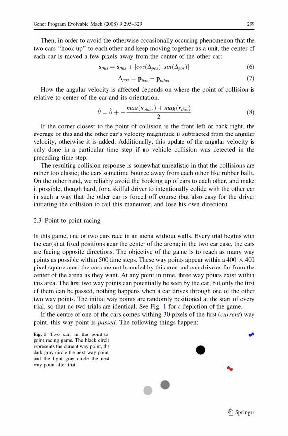
trial, so that no two trials are identical. See Fig. 1 for a depiction of the game.

If the centre of one of the cars comes withing 30 pixels of the first (current) way

point, this way point is passed. The following things happen:

Fig. 1 Two cars in the point-to-point racing game. The black circlerepresents the current way point, thedark gray circle the next way point,and the light gray circle the nextway point after that


123

– The passed way points count (the score) for that car’s driver increases by 1.

– The current way point disappears, the second way point becomes current, and

the third way point becomes second.

– A new third way point is generated, by drawing its x and y coordinates from a

uniform distribution limited by 0 and 400.

The objective of the game is simply to reach as many way points as possible

within the time limits, on a single trial or averaged over several trials. With only one

car this mainly comes down to maneuvering the car to the current way point as fast

as possible, but some foresight is needed as the way points are not navigated to in

isolation. With two cars on the same track considerably more complexity is added.

The following is a probably incomplete breakdown of the tasks that need to be

mastered, in order of increasing difficulty, in order to win the game in direct

competition with a sophisticated opponent:

1. Reach the current way point. This requires not only driving towards the correct

way point, but also not overshooting it. A driver that constantly accelerates

(issues the forward command) while steering in the direction of the way point

will end up ‘‘orbiting’’ the way point at one time or another, as the grip of the

tyres is limited and decreases with speed.

2. Reach the current way point fast. While it is possible to solve the preceding task

by just driving very slowly (through only accelerating when the speed of the car

is below a low threshold) and steering in the direction that the angle between

the direction of the car and the way point is smallest, it would obviously take a

long time to reach the way point that way. As a driver that on average reaches

way points faster will win over a slower driver, it is necessary to drive at as high

speed as possible without overshooting the way point.

3. Reach the current way point in such a way that the next way point can be

reached quickly. For example, it is usually a bad idea to reach the current way

point going at full speed away from the next way point, which will soon be the

current way point. In such cases, it often pays off to start braking before

reaching the current way point, and trading off a slight delay in reaching that

way point with being able to reach the next way point much faster.

4. Predict which car will reach the current way point first. If a driver can predict

whether his car or the opponents’ car will reach the next way point first, he can

take appropriate action. An obvious response is aiming for the next way point

instead, and waiting for it to become the current way point; in that way he only

misses one way point, instead of risking to miss two way points. However,

knowing for sure which car will reach the current way point first involves

understanding not only the dynamics of the car simulation, but also the

behaviour of the other driver. What if he decides that he is not going to make it

first to the current way point, and goes for the next way point directly himself?

5. Use collisions to one’s advantage. There are situations when it is advantageous

to be able to knock the opponent off course. For example in case the opponent

would get to the current way point first, due to higher speed, but it is possible to

get in the way of the opponent and collide with him so that he misses the way

point. It could even be possible to ‘‘steal’’ some of his velocity this way, and use


123

it to get oneself to the current way point faster. Conversely, if the opponent has

figured out how to disrupt one’s path through intentional collisions, it becomes

important to learn how to avoid such collisions.

3 Interface, default controllers and scoring

Controllers interact with the game either directly, through a Java interface, or via a

TCP/IP protocol. This makes it possible to submit controllers written in any

programming language capable of network communication and producing execu-

tables that work on standard desktop operating systems; however, in the CEC

competition all submitted controllers were written in pure Java. Regardless of which

communication method was chosen, the controllers can access (but obviously not

modify) the full state of the game in a third-person representation similar to that

used by the game internally. Additionally, controllers can access much of the

information in a more convenient first-person perspective, e.g. angles and distances

in the frame of reference of the car. If the controller is written in Java, it implements

a simple Controller interface, which specifies a method called control that at every

time step gets passed an object instantiating the interface SensorModel. The

controller can then query this object for any first- or third-person information it

wants, and can also retrieve a copy of the game engine itself with which it can

simulate the outcome of actions.

Regardless of the interface type or the information used by the controller, the

controller always returns two integers signifying the motor command (backward,

neutral, forward) and the steering command (left, center, right).

In addition to the game itself, the simplerace source code package, available for free

download from the competition web page, contains two sample learning algorithms

and a number of sample controllers. Both the sample algorithms and controllers are in

some form reused in several of the contributions, and some of the controllers were used

in the competitionscore scoring function used for ranking the controllers.

The two sample learning algorithms that are provided are a (15 + 15) evolution

strategy and a TD(0) temporal difference learner. These algorithms can then be

combined with either state-value-based or direct-action controller representations

based on perceptrons or feedforward neural networks (MLPs). The evolution strategy

can further be combined with controller representations based on recurrent neural

networks or expression trees (as are commonly used in genetic programming). The

direct-action controller representations use the following state representation as

inputs to their neural network or possible terminals in a GP tree: speed of the own

vehicle, angle to current way point, distance to current way point, angle to next way

point, distance to next way point, angle to other vehicle and distance to other vehicle.

This set of inputs, while rather incomplete when compared to the full state of the

system, has proved to be a good fit for many types of parameterized function

representations, making relatively good driving easy to learn.

Apart from these evolvable controller substrates, three hard-coded heuristic

controllers are provided.


123

– GreedyController is as simple as a controller can be: it always outputs the motor

command ‘‘forward’’, and depending on whether the angle to the current way

point is negative or positive, outputs right or left a steering command. This

controller is very ineffective. It typically overshoots way points because it is

driving too fast, and frequently ends up ‘‘orbiting’’ a way point, meaning that it

gets stuck circling the way point, as it cannot slow down.

– HeuristicSensibleController aims straight for the current way point just like the

GreedyController, but limits its speed to 7 pixels per time step, a moderate

speed. If the speed is below the limit, it issues the forward motor command, but

if it’s above the limit it issues the neutral driving command. This controller

performs much better than the GreedyController when driving a track on its

own, but with another car on the track it typically loses out, as it aims for the

current way point even if the other car is bound to get there first. It also has some

problems with orbiting.

– HeuristicCombinedController is a rather more complex beast. Its behaviour

differs depending on whether the car it is controlling is currently closer to the

current way point than the other car. If so, it behaves like the HeuristicSen-sibleController. If not, it enters ‘‘underdog’’ mode and steers toward the nextway point, with the same speed limit as the aforementioned controller. However,

when it gets close to that way point, it stops; when in underdog mode, it

decreases its speed proportionally to the distance to the next way point. This

controller behaves much better than the HeuristicSensibleController in head-to-

head races, and is typically a match for an intermediate human player of the

game. However, it can be beaten by a learned controller, as we shall see.

This brings us to the CompetitionScore metric, which is the metric used to rank

the submitted controllers before the final tournament. This metric is defined as the

mean fitness of 500 trials in each of three conditions: on its own, versus a

HeuristicSensibleController and versus a HeuristicCombinedController. This

means that to achieve a high CompetitionScore, a controller needs to perform well

on its own, as well as against a weak and an intermediate controller, and so can’t

assume too much about the behaviour of its opponent.

4 Competition organization

The competition was organized as described in this section. Approximately four

months before the competition event at the CEC conference, the software package

was made available for free downloading from the competition web site. The

software package contains the racing game itself as well as sample controllers and

learning algorithms; the web page contains simple instructions for e.g. training your

first controller, playing a manual game against it, measuring its CompetitionScore

etc. Full Java source code, as well as compiled class files, is provided for all

software. This is done in order to maximize the competitors’ understanding of the

domain, and facilitate for people who prefer to work in another programming

language than Java to translate their algorithms into their own frameworks. While it

may be argued that the details of the model should be hidden to the competitors in


123

order to make the competition more about learning algorithms and less about clever

human use of domain knowledge, this is in practice very hard to do; a determined

individual could always decompile and de-obfuscate compiled classes. Addition-

ally, the dynamics are to our best knowledge too complicated to allow for any

complete analytical solution to the problem.

Each submitted entry was scored by the organizers using the standard

CompetitionScore method (participants were encouraged to provide their figure

for the score of their controller, to make sure that the organizers ran the controller

correctly) and the score and controller were as soon as possible made available on

the competition web page. As participants were encouraged to submit source code

for their controllers, this meant that for all except one controller, full source code is

available from the website; for the last controller, only binaries (class files) are

available. The reason the submitted controllers were put up on the website was to

give the competition participants good opponents to train their own controllers

against; the reason the source code was made available as well was to increase the

usefulness of the outcomes of the competition. We reasoned that through being able

to access the source code itself, more can be learnt than just reading the description

of a controller in a paper.

Participants were permitted to resubmit their controllers an unlimited number of

times, and also to submit more than one controller from the same team, as long as

they could show that there were significant differences between the controllers.

While no team took advantage of the possibility to enter more than one controller in

the competition, most participants did update their submissions several times. This

was especially true in the last few days of the competition, when the top few teams

tried their best to outdo each other’s efforts, submitting a stream of updates to their

controllers that were in part general improvements, in part tuned specifically to beat

the other controllers in the top four. However, the team that eventually won the

competition submitted their controller on the very day of the deadline, thus not giving

any of the other teams a chance to tailor their controllers to it, while themselves being

able to take the behaviour of the already submitted controllers into account.

After the deadline, the four top-scoring controllers were all played out against

each other, and the controller that beat most of the other controllers in head-to-head

races won the competition as a whole. The results were presented as part of the

(well-attended) special session on Evolutionary Computation in Games of the

Congress on Evolutionary Computation, and the winners were also awarded a cash

prize at the conference banquet.

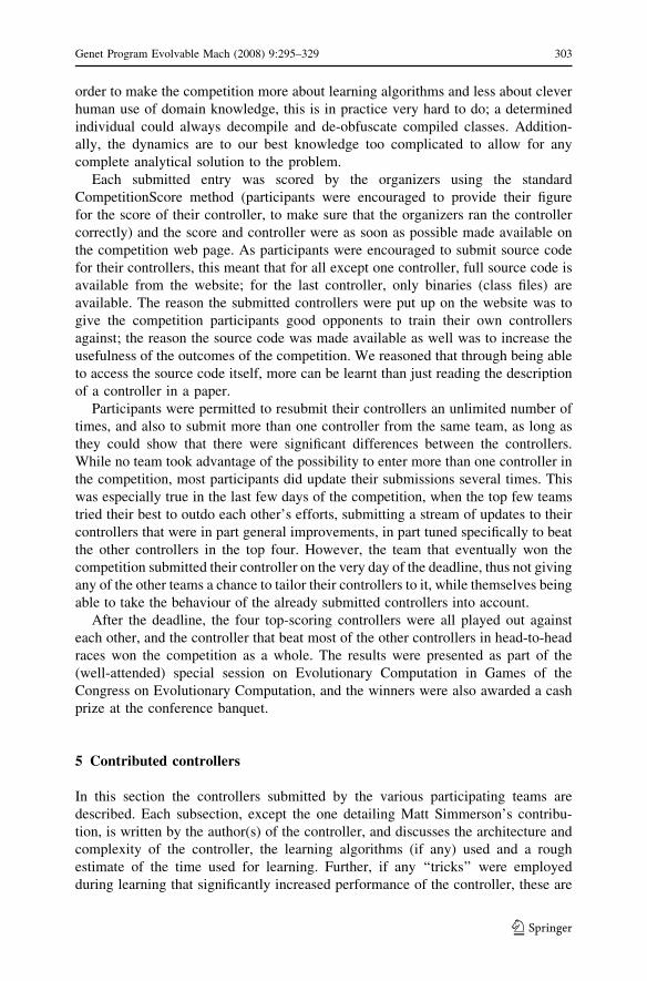
5 Contributed controllers

In this section the controllers submitted by the various participating teams are

described. Each subsection, except the one detailing Matt Simmerson’s contribu-

tion, is written by the author(s) of the controller, and discusses the architecture and

complexity of the controller, the learning algorithms (if any) used and a rough

estimate of the time used for learning. Further, if any ‘‘tricks’’ were employed

during learning that significantly increased performance of the controller, these are


123

explained. The sections are ordered by the controllers’ competition scores, in

ascending order; this order is chosen because the higher scoring controllers are

typically more complex than the lower-scoring ones, and tend to reuse and refine the

techniques introduced in the lower-scoring controllers.

5.1 Matt Simmerson

NEAT (Neuro Evolving Augmenting Topologies) is a methodology for efficiently

evolving Neural Networks through complexification developed by Stanley and

Miikkulainen [3]. It uses a genetic representation that enables principled crossover

of different topologies. NEAT has an elaborate mechanism for protecting structural

innovation using speciation. The networks start minimally and grow in complex-

ity(nodes,links) incrementally. For more details about NEAT and its applications in

various domains, see [4].

For this controller, a rather straightforward approach was taken, with a

‘‘standard’’ set of inputs (as described in section 3) interfaced to a single network,

and the outputs interpreted as driving and steering commands. The NEAT4Jimplementation of NEAT was used for the training.3 We currently don’t have any

information on the complexity of the evolved neural network.

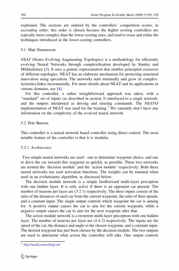
5.2 Pete Burrow

This controller is a neural network based controller using direct control. The most

notable feature of the controller is that it is modular.

5.2.1 Architecture

Two simple neural networks are used - one to determine waypoint choice, and one

to drive the car towards this waypoint as quickly as possible. These two networks

are termed the ‘decision module’ and the ‘action module’ respectively. Both these

neural networks use tanh activation functions. The weights can be mutated when

used in an evolutionary algorithm, as discussed below.

The decision module network is a simple feedforward multi-layer perceptron

with one hidden layer. It is only active if there is an opponent car present. The

number of neurons per layer are (3 2 1) respectively. The three inputs consist of the

ratio of the distances of each car from the current waypoint, the ratio of their speeds,

and a constant input. The single output controls which waypoint the car is aiming

for. A positive output causes the car to aim for the current waypoint, while a

negative output causes the car to aim for the next waypoint after that.

The action module network is a recurrent multi-layer perceptron with one hidden

layer. The number of neurons per layer are (4 4 2) respectively. The inputs are the

speed of the car, the distance and angle to the chosen waypoint, and a constant input.

The desired waypoint has just been chosen by the decision module. The two outputs

are used to determine what action the controller will take. One output controls

3 http://neat4j.sourceforge.net


123

http://neat4j.sourceforge.net

direction, the other whether to accelerate forward, backward or not at all. Each of

the three actions are determined by whether the output is less than -0.3, greater

than 0.3, or somewhere in the middle.

5.2.2 Training

Training of the controller was performed using evolutionary learning. There was

mutation but no crossover. The two neural networks were trained separately.

The action module was trained first using a standard (15 + 15) evolution

strategy. The population of controllers was evolved on the single controller case,

where there was no other car to compete against. This network was evolved for 500

generations. This produced a controller with good solo performance.

The decision module was trained using our version of the N-strikes-out algorithm

[5, 6]. A population of 30 individuals were evolved while competing to see which

performed best against a fixed opponent in the two car case. The provided

HeuristicSensibleController was used as the fixed opponent. The weights on the

action module were kept constant during this process - only the weights of the

decision module were subject to mutation. Evolution was run for the equivalent of

500 generations, which was enough to produce a controller that performed well with

the CompetitionScore class.

5.2.3 Complexity

In terms of size and complexity, the controller is fairly simple. The controller is

about 100 lines of code, not including the provided MLP and RMLP neural network

classes. In total there are 16 neurons, and 48 connections/weights. There is no

internal simulation, it is simply a direct action controller.

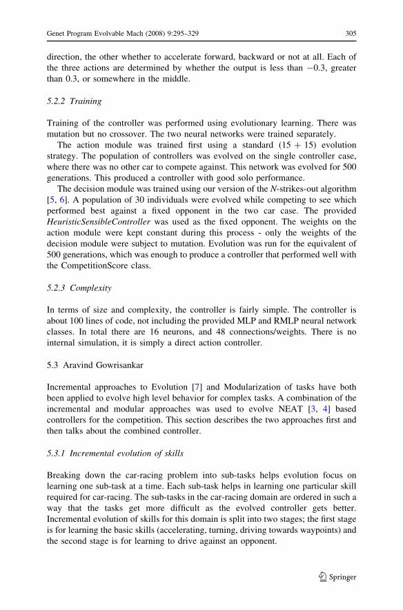
5.3 Aravind Gowrisankar

Incremental approaches to Evolution [7] and Modularization of tasks have both

been applied to evolve high level behavior for complex tasks. A combination of the

incremental and modular approaches was used to evolve NEAT [3, 4] based

controllers for the competition. This section describes the two approaches first and

then talks about the combined controller.

5.3.1 Incremental evolution of skills

Breaking down the car-racing problem into sub-tasks helps evolution focus on

learning one sub-task at a time. Each sub-task helps in learning one particular skill

required for car-racing. The sub-tasks in the car-racing domain are ordered in such a

way that the tasks get more difficult as the evolved controller gets better.

Incremental evolution of skills for this domain is split into two stages; the first stage

is for learning the basic skills (accelerating, turning, driving towards waypoints) and

the second stage is for learning to drive against an opponent.


123

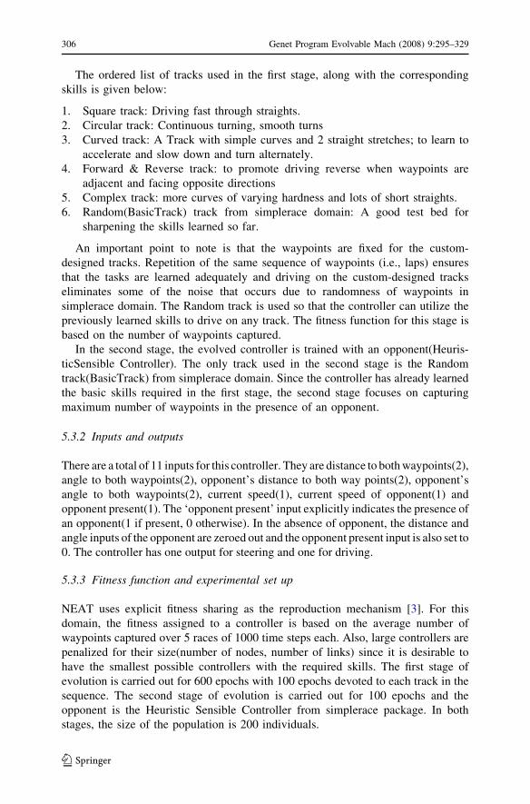
The ordered list of tracks used in the first stage, along with the corresponding

skills is given below:

1. Square track: Driving fast through straights.

2. Circular track: Continuous turning, smooth turns

3. Curved track: A Track with simple curves and 2 straight stretches; to learn to

accelerate and slow down and turn alternately.

4. Forward & Reverse track: to promote driving reverse when waypoints are

adjacent and facing opposite directions

5. Complex track: more curves of varying hardness and lots of short straights.

6. Random(BasicTrack) track from simplerace domain: A good test bed for

sharpening the skills learned so far.

An important point to note is that the waypoints are fixed for the custom-

designed tracks. Repetition of the same sequence of waypoints (i.e., laps) ensures

that the tasks are learned adequately and driving on the custom-designed tracks

eliminates some of the noise that occurs due to randomness of waypoints in

simplerace domain. The Random track is used so that the controller can utilize the

previously learned skills to drive on any track. The fitness function for this stage is

based on the number of waypoints captured.

In the second stage, the evolved controller is trained with an opponent(Heuris-

ticSensible Controller). The only track used in the second stage is the Random

track(BasicTrack) from simplerace domain. Since the controller has already learned

the basic skills required in the first stage, the second stage focuses on capturing

maximum number of waypoints in the presence of an opponent.

5.3.2 Inputs and outputs

There are a total of 11 inputs for this controller. They are distance to both waypoints(2),

angle to both waypoints(2), opponent’s distance to both way points(2), opponent’s

angle to both waypoints(2), current speed(1), current speed of opponent(1) and

opponent present(1). The ‘opponent present’ input explicitly indicates the presence of

an opponent(1 if present, 0 otherwise). In the absence of opponent, the distance and

angle inputs of the opponent are zeroed out and the opponent present input is also set to

0. The controller has one output for steering and one for driving.

5.3.3 Fitness function and experimental set up

NEAT uses explicit fitness sharing as the reproduction mechanism [3]. For this

domain, the fitness assigned to a controller is based on the average number of

waypoints captured over 5 races of 1000 time steps each. Also, large controllers are

penalized for their size(number of nodes, number of links) since it is desirable to

have the smallest possible controllers with the required skills. The first stage of

evolution is carried out for 600 epochs with 100 epochs devoted to each track in the

sequence. The second stage of evolution is carried out for 100 epochs and the

opponent is the Heuristic Sensible Controller from simplerace package. In both

stages, the size of the population is 200 individuals.


123

5.3.4 Modular approach to car-racing

The simplest way to decompose the car racing problem is to have two modules—

one for way-point selection and one for navigating to the selected way-point.

5.3.5 Inputs and outputs

The navigator and waypoint chooser have 7 inputs each. The waypoint chooser uses

information (about both players) like current speed and estimated time to travel to each

of the two waypoints for selecting a target waypoint. It has just one output indicating

the selected target waypoint. The navigator takes in the current speed, the distance and

angle to the ‘selected waypoint’ (for both players) as inputs. It has two outputs for

steering and driving. As in the earlier approach, both controllers have the ‘opponent

present’ input which is used to indicate the presence or absence of an opponent.

5.3.6 Fitness functions and experimental setup

In this approach, the navigator and waypoint chooser controllers are evolved

together. During a race, the way-point chooser picks the next way-point and the

navigator drives towards the selected waypoint. This is implemented by having two

populations, one each for the navigator and waypoint chooser. The populations

consist of 200 organisms each and the evolution is carried out for 500 epochs. Each

way-point chooser from the waypoint chooser population is paired up with every

navigator from the navigator population. The fitness of the modular controller has

two components . The first component is a solo race and the second one is with an

opponent. Both components involve 5 races of 1000 time-steps each. The fitness

assigned to the controller is a weighted sum of the waypoints captured in the two

cases. As it is more difficult to drive with an opponent, the waypoints captured while

racing with an opponent are weighed higher than waypoints captured while driving

alone. Also, since the two populations are being evolved simultaneously, fitness

must be assigned to controllers from both populations. Fitness assigned to a

controller from one population(way-point chooser or navigator) is the best fitness

achieved when paired with every controller from other population.

5.3.7 Results

The controller developed using the first approach(Incremental Evolution of Skills)

obtained a credible solo score of 18.1 (Table 1). However, the scores with the

Sensible Heuristic Controller and Combined Heuristic Controller were significantly

lower and hence the overall competition score was lower(14.86). In the second

approach, a modular controller was created specifically to separate the navigation

and waypoint selection tasks. The modular controller, surprisingly failed to perform

as well as the controller created using the former approach. Both the solo

scores(14.76) and the scores while racing with an opponent were lower than

the incrementally evolved controller(discussed in the next sub-section). However,

the controller had a desired behavior of being fast on long straights. For the


123

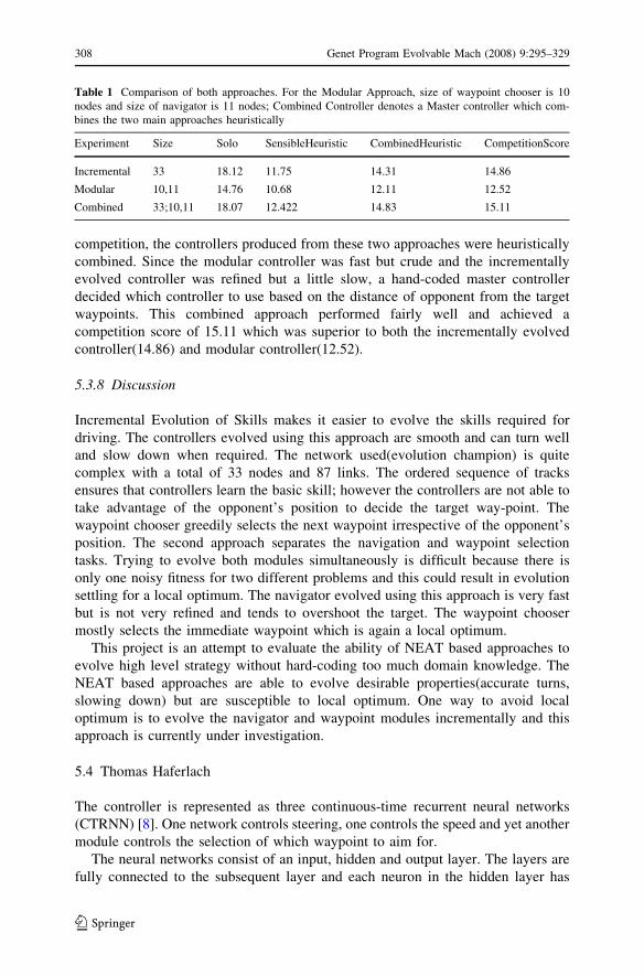
competition, the controllers produced from these two approaches were heuristically

combined. Since the modular controller was fast but crude and the incrementally

evolved controller was refined but a little slow, a hand-coded master controller

decided which controller to use based on the distance of opponent from the target

waypoints. This combined approach performed fairly well and achieved a

competition score of 15.11 which was superior to both the incrementally evolved

controller(14.86) and modular controller(12.52).

5.3.8 Discussion

Incremental Evolution of Skills makes it easier to evolve the skills required for

driving. The controllers evolved using this approach are smooth and can turn well

and slow down when required. The network used(evolution champion) is quite

complex with a total of 33 nodes and 87 links. The ordered sequence of tracks

ensures that controllers learn the basic skill; however the controllers are not able to

take advantage of the opponent’s position to decide the target way-point. The

waypoint chooser greedily selects the next waypoint irrespective of the opponent’s

position. The second approach separates the navigation and waypoint selection

tasks. Trying to evolve both modules simultaneously is difficult because there is

only one noisy fitness for two different problems and this could result in evolution

settling for a local optimum. The navigator evolved using this approach is very fast

but is not very refined and tends to overshoot the target. The waypoint chooser

mostly selects the immediate waypoint which is again a local optimum.

This project is an attempt to evaluate the ability of NEAT based approaches to

evolve high level strategy without hard-coding too much domain knowledge. The

NEAT based approaches are able to evolve desirable properties(accurate turns,

slowing down) but are susceptible to local optimum. One way to avoid local

optimum is to evolve the navigator and waypoint modules incrementally and this

approach is currently under investigation.

5.4 Thomas Haferlach

The controller is represented as three continuous-time recurrent neural networks

(CTRNN) [8]. One network controls steering, one controls the speed and yet another

module controls the selection of which waypoint to aim for.

The neural networks consist of an input, hidden and output layer. The layers are

fully connected to the subsequent layer and each neuron in the hidden layer has

Table 1 Comparison of both approaches. For the Modular Approach, size of waypoint chooser is 10

nodes and size of navigator is 11 nodes; Combined Controller denotes a Master controller which com-

bines the two main approaches heuristically

Experiment Size Solo SensibleHeuristic CombinedHeuristic CompetitionScore

Incremental 33 18.12 11.75 14.31 14.86

Modular 10,11 14.76 10.68 12.11 12.52

Combined 33;10,11 18.07 12.422 14.83 15.11


123

recurrent connections to all of the other neurons in the hidden layer. The inputs are

the speeds and distances of both competitors towards the next waypoint and the

angle and distance of the racer towards the competitor.

The network was evolved with a simplified version of the CoSyNE algorithm,

which uses competitive co-evolution on synapse (network connection) level [9].

Instead of performing crossover between two members of the population, the genes

are permuted amongst all members of the population. Every resulting controller has

a mix of genes from the whole previous population. This lead to a 5–7x increase in

speed of finding a well performing solution in comparison to a genetic algorithm

using regular crossover.

The controller was evolved for 200 generations with a population of 100

networks; several runs with this configuration were made, but fitness never

increased significantly after 200 generations.

5.5 Bob MacCallum

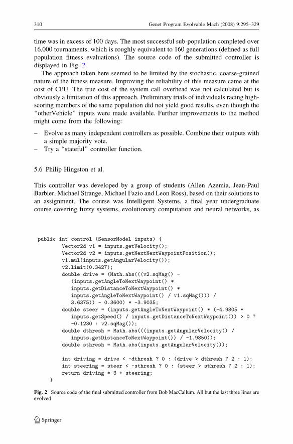
The core logic of the controller was evolved using genetic programming in a

somewhat unorthodox fashion. The code is generated by the grammar-based PerlGP

system [10, 11] as Java source text, which is then compiled and executed through

system calls from Perl. The fitness is ‘‘grepped’’ from the text output of the

simplerace.Stats or CompetitionScore classes.

The controller uses a simple direct control architecture (no state values or internal

simulation) similar to several of the demonstration classes (e.g. simplerace.Percep-

tronController). The only modification to this approach is that the thresholds used to

quantize the ‘‘drive’’ and ‘‘steer’’ outputs are evolved. (The values for ‘‘drive’’ and

‘‘steer’’ are also evolved, of course.) The values are produced by evolved Java code

as follows: Two temporary vector variables v1 and v2 are initialised from one of the

inputs, and then modified by an arbitrary number of vector manipulation statements.

Finally the drive and steer variables and their respective thresholds are assigned by

arbitrary length scalar expressions of Java type ‘‘double’’. These scalar expressions

may contain components derived from vector inputs or temporary variables (e.g.

v1.sqMag()). For convenience, the threshold outputs are wrapped in a Math.abs()

call hardcoded into the grammar. All sensor inputs which do not involve the other

vehicle can contribute to the generation of driving and steering command. The

controller method is stateless (no memory of previous invocations).

Training was performed in two stages. First, a modifed version of simple-

race.Evaluator.evaluateSolo was used which returned the product of the standard

fitness measure and the number of different controller commands used during the

simulation. The purpose of this was to encourage ‘‘interesting’’ controller behaviour

which was not seen prior to the introduction of this fitness function modification.

The number of trials averaged over was also increased to 1000. The second stage of

training used the standard simplerace.CompetitionScore measure (number of

waypoints passed averaged over three races: one solo and two against opponents)

with 2000 trials. The increased number of trials seemed to be needed to provide a

stable measure of performance. Ten experiments were run in parallel with

occasional migration between populations (each of 2000 individuals). Total CPU


123

time was in excess of 100 days. The most successful sub-population completed over

16,000 tournaments, which is roughly equivalent to 160 generations (defined as full

population fitness evaluations). The source code of the submitted controller is

displayed in Fig. 2.

The approach taken here seemed to be limited by the stochastic, coarse-grained

nature of the fitness measure. Improving the reliability of this measure came at the

cost of CPU. The true cost of the system call overhead was not calculated but is

obviously a limitation of this approach. Preliminary trials of individuals racing high-

scoring members of the same population did not yield good results, even though the

‘‘otherVehicle’’ inputs were made available. Further improvements to the method

might come from the following:

– Evolve as many independent controllers as possible. Combine their outputs with

a simple majority vote.

– Try a ‘‘stateful’’ controller function.

5.6 Philip Hingston et al.

This controller was developed by a group of students (Allen Azemia, Jean-Paul

Barbier, Michael Strange, Michael Fazio and Leon Ross), based on their solutions to

an assignment. The course was Intelligent Systems, a final year undergraduate

course covering fuzzy systems, evolutionary computation and neural networks, as

Fig. 2 Source code of the final submitted controller from Bob MacCallum. All but the last three lines areevolved


123

well as touching on ant colony optimisation, particle swarm optimisation, and

artificial life. Students were given six weeks to complete their individual controllers.

They were assessed on the competition score achieved by their controller, and on a

project log in which they recorded their progress. At the end of semester, the authors

of the four best controllers were invited to spend an additional day to work as a

team, putting together a concensus solution to submit to the competition.

The students were provided with the competition code, and an Intelligent

Systems Toolkit created by the lecturer, which is a Java class library that supports

type-1 fuzzy systems, multi-layer perceptrons, and simple evolutionary algorithms.

The Toolkit also makes it simple to tune a fuzzy system or a multi-layer perceptron

using an evolutionary algorithm. Students in this class have varying degrees of

programming skill, from rather poor to very capable. With the combination of the

competition code and the Toolkit, even the most challenged students were able to

create a working controller.

5.6.1 Architecture

The consensus solution used a multi-layer perceptron and a number of fuzzy sub-

systems to perform various tasks:

1. A multi-layer perceptron (MLP) to decide whether or not to try for the next

waypoint;

2. A fuzzy system (DRIFT) to decide whether to start ‘‘drifting’’ (when

approaching a waypoint, at the last moment we turn our steering towards the

next waypoint, thus drifting through the current waypoint);

3. A fuzzy system (SPEED) to control speed;

4. A fuzzy system (STEER) to control steering; and

5. A fuzzy system (STALEMATE) to detect a special kind of stalemate situation,

where the opponent has become ‘‘stuck’’ cycling around the current waypoint, and

we have decided to concede the current waypoint and go to the next waypoint.

In pseudo-code form, the logic of the controller is as follows:

If MLP decides to go for this waypoint or stalemate detected then

angle ¼ angle to this waypoint

distance ¼ distance to this waypoint

else==go for next waypoint

angle ¼ angle to next waypoint

distance ¼ distance to next waypoint

If DRIFT decides it is time to drift then

angle ¼ angle to waypoint after selected waypoint

Calculate SPEED and STEERING and combine these to select the control

action


123

5.6.2 MLP

The architecture of the MLP was this:

– Inputs: (our speed)/(opponent speed), (our distance to the waypoint)/(opponent

distance to waypoint)

– Hidden layers: 1, with 5 hidden units

– Outputs: 2, if first output[ second output go to next waypoint else go to current

waypoint

5.6.3 Fuzzy logic

Fuzzy sets were defined using trapezoidal membership functions. All the fuzzy rules

are Sugeno type fuzzy rules with a constant as the consequent. So an example of a

fuzzy rule might be:

IF distance to waypoint IS medium AND our speed IS very slow THEN

drift = 0

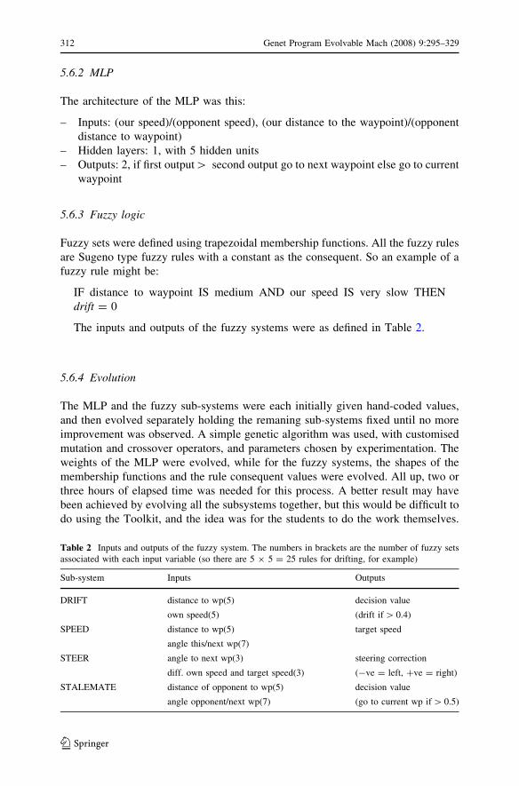
The inputs and outputs of the fuzzy systems were as defined in Table 2.

5.6.4 Evolution

The MLP and the fuzzy sub-systems were each initially given hand-coded values,

and then evolved separately holding the remaning sub-systems fixed until no more

improvement was observed. A simple genetic algorithm was used, with customised

mutation and crossover operators, and parameters chosen by experimentation. The

weights of the MLP were evolved, while for the fuzzy systems, the shapes of the

membership functions and the rule consequent values were evolved. All up, two or

three hours of elapsed time was needed for this process. A better result may have

been achieved by evolving all the subsystems together, but this would be difficult to

do using the Toolkit, and the idea was for the students to do the work themselves.

Table 2 Inputs and outputs of the fuzzy system. The numbers in brackets are the number of fuzzy sets

associated with each input variable (so there are 5 9 5 = 25 rules for drifting, for example)

Sub-system Inputs Outputs

DRIFT distance to wp(5) decision value

own speed(5) (drift if [ 0.4)

SPEED distance to wp(5) target speed

angle this/next wp(7)

STEER angle to next wp(3) steering correction

diff. own speed and target speed(3) (-ve = left, +ve = right)

STALEMATE distance of opponent to wp(5) decision value

angle opponent/next wp(7) (go to current wp if [ 0.5)


123

The aims of our entry into this competition were not scientific, but educational.

Students were very motivated by this task. Some spent much too much time

working on it, and nearly all gained a much more solid understanding of the

methods used. The course received high student ratings and the comments in the

logbooks were almost universally positive. I would heartily recommend setting

student assignments based on competitions in this area, and encourage competition

organisers to keep the entry barrier low by providing simple interfaces.

5.7 Itamar Elhanany and Shay Berant

A direct-critic reinforcement learning (RL)-based controller was implemented using

a feed-forward neural network. The critic was trained to estimate the state-value

function, based on experience initially driven by a heuristic reference controller,

followed by direct interaction with the environment. Training was based on a

model-free temporal difference (TD) approximate dynamic programming frame-

work [12]. While a state-value function-based control suffices for the solo (single-

car) scenario, a higher layer of hard-coded domain knowledge was added to address

the two cars scenario, as outlined below.

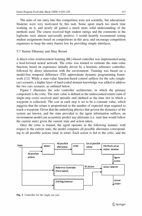
Figure 3 illustrates the solo controller architecture, in which the primary

component is the critic. The state value is defined as the undiscounted return (sum of

single-step costs) received until episodic end (defined as the time slot in which a

waypoint is collected). The cost in each step is set to be a constant value, which

suggests that the return is proportional to the number of expected steps required to

reach a waypoint. Given that the underlying physics that govern the dynamics of the

system are known, and the state provided to the agent information suffices, an

environment model can accurately predict any afterstate (i.e. state that would follow

the current state) given the current state and action taken.

Once the critic is trained, the agent operates in the following manner: with

respect to the current state, the model computes all possible afterstates correspond-

ing to all possible actions (nine in total). Each action is fed to the critic, and the

Fig. 3 Controller for the single-car case


123

action that yields the minimal return (i.e. the minimal expected time to reach the

waypoint) is selected. Critic training was achieved using a temporal difference

learning method in which the state contained information pertaining to the current

waypoint only, and was composed from the following invariant parameters: distance

and angle to next waypoint, car velocity (magnitude and angle), slip angle and

angular velocity. The weights of the neural network were updated using a standard

backpropagation algorithm, with the error defined as the TD error:

dt ¼ rtþ1 þ cVtðstþ1Þ � VtðstÞ ¼r þ Vtðstþ1Þ � VtðstÞ not at waypoint

r � VtðstÞ at waypoint

�ð9Þ

where dt,rt and Vt(s) are the error, reward (cost) and estimated value of state s at

time t, respectively, and c = 1 is the discount-rate parameter.

In many real-life applications, training a system from scratch proves impractical

from a running-time perspective. To that end, a unique apprenticeship learning

scheme was employed in which the critic was initially trained to learn the state-

action value function of a reference, heuristic controller. The latter comprised of a

simplistic rule-based scheme. In a subsequent stage, the agent improved its

proficiency by modifying its value function estimation, based on experience

acquired through interaction with its environment. Control is gradually shifted to the

agent using the minimum return action selection method as described above,

allowing the agent to explore new states. Based on the policy improvement theorem

in RL [12], the agent continuously improves its policy by greedily following the

current policy and adjusting its value function estimation, accordingly. The critic

ends up learning its own improved policy’s value function.

As with many other controllers applied to this task, while testing the agent it was

observed that an ‘orbiting’ phenomenon occurred. This resulted from over-speeding

in situations where speed limitations should be enforced by the agent. A heuristic

framework for overcoming orbiting at any radius, was devised in which an

approximated measure, lt, of the recent average distance from the waypoint and its

variation, rt, were continuously calculated in the following manner:

ltþ1 ¼ a � lt þ ð1� aÞ � dtþ1

rtþ1 ¼ a � rt þ ð1� aÞ � ltþ1 � dtþ1

�� orbiting if rt \ rthreshold

ð10Þ

A small standard deviation (less than a predefined threshold) served as an

indication for orbiting. When the latter was detected, control was switched to the

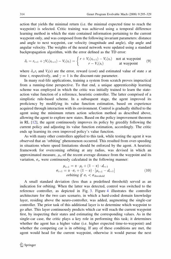
reference controller, as depicted in Fig. 3. Figure 4 illustrates the controller

architecture for the two cars scenario, in which a hard-coded domain knowledge

layer, residing above the neuro-controller, was added, augmenting the single-car

controller. The prior task of this additional layer is to determine which waypoint to

go after. This layer continuously predicts which car will reach the current waypoint

first, by inspecting their states and estimating the corresponding values. As in the

single-car case, the critic plays a key role in performing this task; it determines

whether the agent has a higher value (i.e. higher expected time-to-waypoint) and

whether the competing car is in orbiting. If any of these conditions are met, the

agent would head for the current waypoint, otherwise it would pursue the next


123

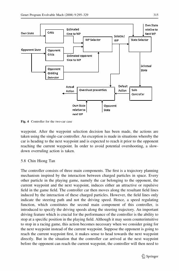
waypoint. After the waypoint selection decision has been made, the actions are

taken using the single-car controller. An exception is made in situations whereby the

car is heading to the next waypoint and is expected to reach it prior to the opponent

reaching the current waypoint. In order to avoid potential overshooting, a slow-

down overruling action is taken.

5.8 Chin Hiong Tan

The controller consists of three main components. The first is a trajectory planning

mechanism inspired by the interaction between charged particles in space. Every

other particle in the playing game, namely the car belonging to the opponent, the

current waypoint and the next waypoint, induces either an attractive or repulsive

field in the game field. The controller car then moves along the resultant field lines

induced by the interaction of these charged particles. However, the field lines only

indicate the steering path and not the driving speed. Hence, a speed regulating

function, which constitutes the second main component of this controller, is

introduced to specify the driving speeds along the steering trajectory. An important

driving feature which is crucial for the performance of the controller is the ability to

stop at a specific position in the playing field. Although it may seem counterintuitive

to stop in a racing game, this action becomes necessary when we consider going for

the next waypoint instead of the current waypoint. Suppose the opponent is going to

reach the current waypoint first, it makes sense to head towards the next waypoint

directly. But in the situation that the controller car arrived at the next waypoint

before the opponent can reach the current waypoint, the controller will then need to

Fig. 4 Controller for the two-car case


123

stop the car at the next waypoint and wait until it becomes activated. The third

component is a predictive module that chooses which waypoint to go for. By

observing the state of the game area, the controller predicts which car will reach the

current waypoint first. In the event that the opponent is predicted to be faster to the

current waypoint, the controller should then direct the car towards the next waypoint

instead and vice versa.

5.8.1 Evolution

A (25, 25) ES running for 200 generations was used as a training method for the

controller. Each individual is evaluated against the HeuristicSensibleController,

which was a standard controller used in CompetitionScore, for 5 rounds of

competition, followed by 5 rounds of competitive coevolution against another

individual from the population. The fitness function was defined as number of

waypoints the controller collected averaged over the 10 rounds of gameplay. No solo

training was used during the training. Elitism was implemented by retaining the best 4

individuals of each generation. Each chromosome was encoded with a total of 11 real

valued variables, 6 from force field component, 4 from speed regulation component

and 1 additional variable which encode the threshold for reversing driving.

5.8.2 Force field trajectory

The direction of the resulting force field vector at the position of the controlled car

determines the direction in which the car should be steered and the equation for the

force field induced by each particle in the game arena is as follows:

Ei ¼ qirpi r; i ¼ fother;wp1;wp2g ð11Þ

The three particles in the games arena are represented in the set i where other is the

opponent vehicle, wp1 is the current waypoint, wp2 is the next waypoint, Ei is the field

vector induced by the point particle i, qi is the charge of particle i, r is the distance from

the particle with charge qi and the evaluation point, pi is the power factor of the

distance r and r is the unit vector pointing from the particle with charge qi to the

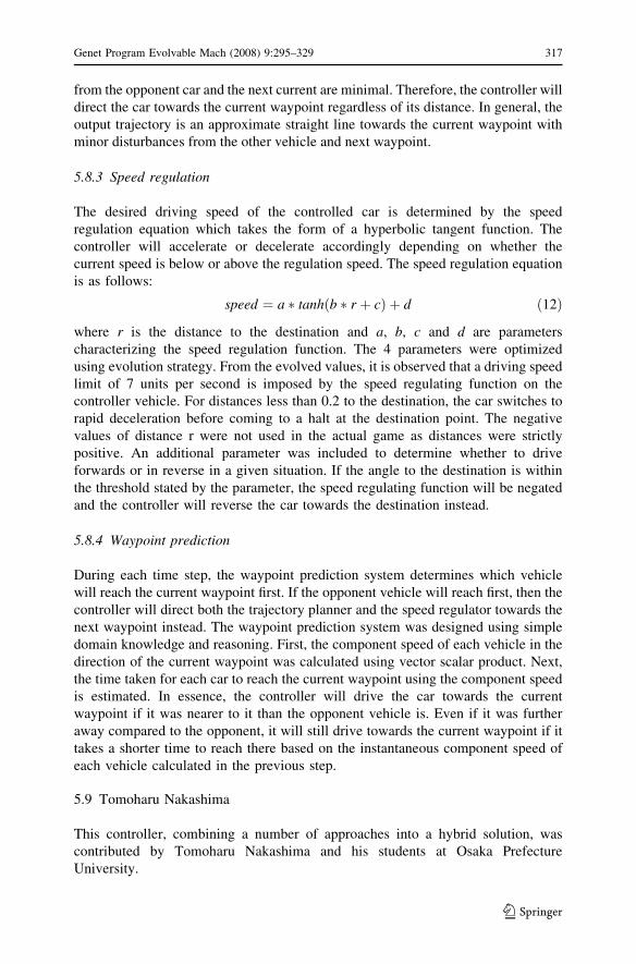
evaluation point. The variables qi and pi for the opponent car, the current waypoint and

the next waypoint were optimized using evolution strategy. The controller car was

considered a point positive charge in calculations in order to evaluate the resultant

force exerted on the controller car. The evolved values are presented in Table 3. All

forces acting on the car are attractive in nature since all qi values turned out to be

negative. The field strength of the current waypoint is at least 10 times larger than that

of the opponent car and the next waypoint within the range of the game area. This

implies the controller car is strongly attracted to the current waypoint while the effects

Table 3 Evolved force field

parameters of best individuali other wp1 wp2

qi -0.02803 -0.896679 -0.063289

pi -0.10153 -0.08817 -0.377045


123

from the opponent car and the next current are minimal. Therefore, the controller will

direct the car towards the current waypoint regardless of its distance. In general, the

output trajectory is an approximate straight line towards the current waypoint with

minor disturbances from the other vehicle and next waypoint.

5.8.3 Speed regulation

The desired driving speed of the controlled car is determined by the speed

regulation equation which takes the form of a hyperbolic tangent function. The

controller will accelerate or decelerate accordingly depending on whether the

current speed is below or above the regulation speed. The speed regulation equation

is as follows:

speed ¼ a � tanhðb � r þ cÞ þ d ð12Þ

where r is the distance to the destination and a, b, c and d are parameters

characterizing the speed regulation function. The 4 parameters were optimized

using evolution strategy. From the evolved values, it is observed that a driving speed

limit of 7 units per second is imposed by the speed regulating function on the

controller vehicle. For distances less than 0.2 to the destination, the car switches to

rapid deceleration before coming to a halt at the destination point. The negative

values of distance r were not used in the actual game as distances were strictly

positive. An additional parameter was included to determine whether to drive

forwards or in reverse in a given situation. If the angle to the destination is within

the threshold stated by the parameter, the speed regulating function will be negated

and the controller will reverse the car towards the destination instead.

5.8.4 Waypoint prediction

During each time step, the waypoint prediction system determines which vehicle

will reach the current waypoint first. If the opponent vehicle will reach first, then the

controller will direct both the trajectory planner and the speed regulator towards the

next waypoint instead. The waypoint prediction system was designed using simple

domain knowledge and reasoning. First, the component speed of each vehicle in the

direction of the current waypoint was calculated using vector scalar product. Next,

the time taken for each car to reach the current waypoint using the component speed

is estimated. In essence, the controller will drive the car towards the current

waypoint if it was nearer to it than the opponent vehicle is. Even if it was further

away compared to the opponent, it will still drive towards the current waypoint if it

takes a shorter time to reach there based on the instantaneous component speed of

each vehicle calculated in the previous step.

5.9 Tomoharu Nakashima

This controller, combining a number of approaches into a hybrid solution, was

contributed by Tomoharu Nakashima and his students at Osaka Prefecture

University.


123

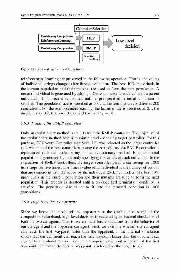
5.9.1 Low-level decision making

For the low-level decision making of our controller, we mainly use two neural

networks with some exception handling. One neural network is a multi-layered

perceptron (MLP) with a 6-9-1 topology, and the other is a recurrent multi-layer

perceptron (RMLP) with a 6-10-9 topology. The ten hidden units of the RMLP are

connected to each other. The input information includes the distance to the first

waypoint, the relative angle to the first waypoint, the distance to the second

waypoint, the relative angle to the second waypoint, and orthogonal components of

the car velocity. We generate the input vector for the MLP from the estimation of

the situation two steps ahead assuming that the car agent performs an action to

evaluate twice. The output of the MLP represents the value of the next state. The

best direction with the largest value is selected as the action of the next time step.

For the RMLP, the action that corresponds to the firing output unit with the largest

value is the action selected by the RMLP controller. The same input vector as in the

case of the MLP is used for the RMLP. For the exception handling, we use

HeuristicCombinedController. The HeuristicCombinedController in this case also

overrides the high-level decision (i.e., the target waypoint). This controller is used in

some special situations where the two neural networks do not work properly. If the

car agent is not in such an emergency, then one of the two controllers is selected

based on the car agents situation. The final action (i.e., one of the possible nine

directions) is determined according to the selected controller. The following are the

selection rules of a controller for low-level decision making:

1. Hand-coded controller that aims at the first waypoint, if the car agent is out of

the main field,

2. Hand-coded controller that aims at the second waypoint, if the high-level

decision is for the second waypoint and the distance between the car agent and

the second waypoint is less than 0.15,

3. RMLP controller, if the distance between the car agent and the first waypoint is

less than 0.6 and the magnitude of the car velocity is less than 5.0,

4. MLP controller, otherwise.

The above selection rules are generated from trial-and-error using the domain

knowledge. Figure 5 illustrates the decision making process for low-level actions.

5.9.2 Training the MLP controller

We trained the MLP controller by the combination of an evolutionary method and a

reinforcement learning method. The reinforcement learning is applied to each

individual during the fitness evaluation. An individual is represented by a real-coded

string of the network weights of an MLP. First, an initial population is generated by

randomly specifying the value of weights of each individual. Next, each individual

is evaluated within a solo car race (i.e., without any opponent car agent) for 1000

time steps. During the evaluation, the weight of the network is modified by temporal

difference learning. The fitness value of an individual is calculated as an average

score for five solo car racings. The weights of the networks modified by the


123

reinforcement learning are preserved in the following operation. That is, the values

of individual strings changes after fitness evaluation. The best 10% individuals in

the current population and their mutants are used to form the next population. A

mutant individual is generated by adding a Gaussian noise to each value of a parent

individual. This process is iterated until a pre-specified terminal condition is

satisfied. The population size is specified as 50, and the termination condition is 200

generations. For the reinforcement learning, the learning rate is specified as 0.1, the

discount rate 0.8, the reward 0.0, and the penalty -1.0.

5.9.3 Training the RMLP controller

Only an evolutionary method is used to train the RMLP controller. The objective of

the evolutionary method here is to mimic a well-behaving target controller. For this

purpose, ECUNeuralController (see Sect. 5.6) was selected as the target controller

as it was one of the best controllers among the competitors. An RMLP controller is

represented as a real-coded string in the evolutionary method. First, an initial

population is generated by randomly specifying the values of each individual. In the

evaluation of RMLP controllers, the target controller plays a car racing for 1000

time steps for five times. The fitness value of an individual is the number of actions

that are coincident with the action by the individual RMLP controller. The best 10%

individuals in the current population and their mutants are used to form the next

population. This process is iterated until a pre-specified termination condition is

satisfied. The population size is set to 50 and the terminal condition is 1000

generations.

5.9.4 High-level decision making

Since we know the model of the opponents in the qualification round of the

competition beforehand, high-level decision is made using an internal simulation of

both the two car agents. That is, we estimate future situations from the behavior of

our car agent and the opponent car agent. First, we examine whether our car agent

can reach the first waypoint faster than the opponent. If the internal simulation

shows that our car agent can reach the first waypoint faster than the opponent car

agent, the high-level decision (i.e., the waypoint selection) is to aim at the first

waypoint. Otherwise the second waypoint is selected as the target to go.

Fig. 5 Decision making for low-level actions


123

In the case where the model of opponent car agents is not known beforehand, an

adaptive HeuristicCombinedController is assumed to be the opponent car agent in

the internal simulation. The adaptive HeuristicCombinedController is an extended

version of HeuristicCombinedController that also internally examine whether it can

reach the first waypoint faster than its opponent or not. In the internal simulation of

the adaptive HeuristicCombinedController, the adaptive HeuristicCombinedCon-

troller can move twice with the probability p. The value of p is modified so that the

movement estimation of the opponent car agent is as correct as possible. If the

estimate of the opponent car agent in the internal simulation is faster than its real

move, the value of p is decreased. On the other hand, the value of p is increased if

the real opponent car agent moves faster than the estimation.

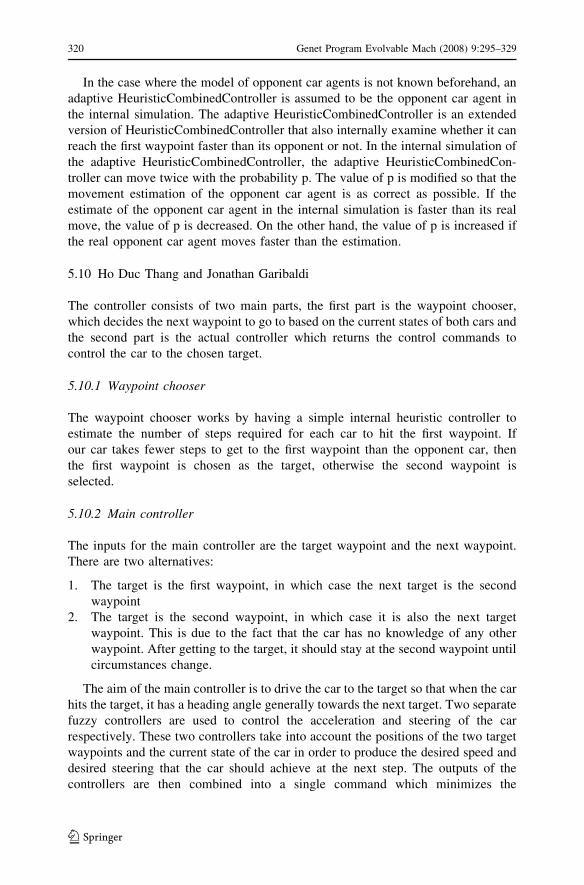
5.10 Ho Duc Thang and Jonathan Garibaldi

The controller consists of two main parts, the first part is the waypoint chooser,

which decides the next waypoint to go to based on the current states of both cars and

the second part is the actual controller which returns the control commands to

control the car to the chosen target.

5.10.1 Waypoint chooser

The waypoint chooser works by having a simple internal heuristic controller to

estimate the number of steps required for each car to hit the first waypoint. If

our car takes fewer steps to get to the first waypoint than the opponent car, then

the first waypoint is chosen as the target, otherwise the second waypoint is

selected.

5.10.2 Main controller

The inputs for the main controller are the target waypoint and the next waypoint.

There are two alternatives:

1. The target is the first waypoint, in which case the next target is the second

waypoint

2. The target is the second waypoint, in which case it is also the next target

waypoint. This is due to the fact that the car has no knowledge of any other

waypoint. After getting to the target, it should stay at the second waypoint until

circumstances change.

The aim of the main controller is to drive the car to the target so that when the car

hits the target, it has a heading angle generally towards the next target. Two separate

fuzzy controllers are used to control the acceleration and steering of the car

respectively. These two controllers take into account the positions of the two target

waypoints and the current state of the car in order to produce the desired speed and

desired steering that the car should achieve at the next step. The outputs of the

controllers are then combined into a single command which minimizes the


123

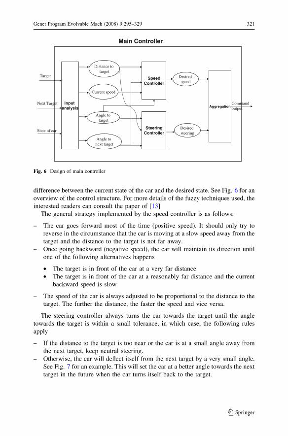
difference between the current state of the car and the desired state. See Fig. 6 for an

overview of the control structure. For more details of the fuzzy techniques used, the

interested readers can consult the paper of [13]

The general strategy implemented by the speed controller is as follows:

– The car goes forward most of the time (positive speed). It should only try to

reverse in the circumstance that the car is moving at a slow speed away from the

target and the distance to the target is not far away.

– Once going backward (negative speed), the car will maintain its direction until

one of the following alternatives happens

• The target is in front of the car at a very far distance

• The target is in front of the car at a reasonably far distance and the current

backward speed is slow

– The speed of the car is always adjusted to be proportional to the distance to the

target. The further the distance, the faster the speed and vice versa.

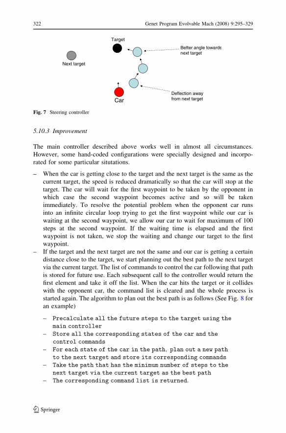
The steering controller always turns the car towards the target until the angle

towards the target is within a small tolerance, in which case, the following rules

apply

– If the distance to the target is too near or the car is at a small angle away from

the next target, keep neutral steering.

– Otherwise, the car will deflect itself from the next target by a very small angle.

See Fig. 7 for an example. This will set the car at a better angle towards the next

target in the future when the car turns itself back to the target.

Inputanalysis

SpeedController

SteeringController

AggregationCommandoutput

Target

Next Target

State of car

Main Controller

Distance totarget

Current speed

Angle totarget

Angle tonext target

Desiredspeed

Desiredsteering

Fig. 6 Design of main controller


123

5.10.3 Improvement

The main controller described above works well in almost all circumstances.

However, some hand-coded configurations were specially designed and incorpo-

rated for some particular situtations.

– When the car is getting close to the target and the next target is the same as the

current target, the speed is reduced dramatically so that the car will stop at the

target. The car will wait for the first waypoint to be taken by the opponent in

which case the second waypoint becomes active and so will be taken

immediately. To resolve the potential problem when the opponent car runs

into an infinite circular loop trying to get the first waypoint while our car is

waiting at the second waypoint, we allow our car to wait for maximum of 100

steps at the second waypoint. If the waiting time is elapsed and the first

waypoint is not taken, we stop the waiting and change our target to the first

waypoint.

– If the target and the next target are not the same and our car is getting a certain

distance close to the target, we start planning out the best path to the next target

via the current target. The list of commands to control the car following that path

is stored for future use. Each subsequent call to the controller would return the

first element and take it off the list. When the car hits the target or it collides

with the opponent car, the command list is cleared and the whole process is

started again. The algorithm to plan out the best path is as follows (See Fig. 8 for

an example)

– Precalculate all the future steps to the target using the

main controller

– Store all the corresponding states of the car and the

control commands

– For each state of the car in the path; plan out a new path

to the next target and store its corresponding commands

– Take the path that has the minimum number of steps to the

next target via the current target as the best path

– The corresponding command list is returned:

Fig. 7 Steering controller


123

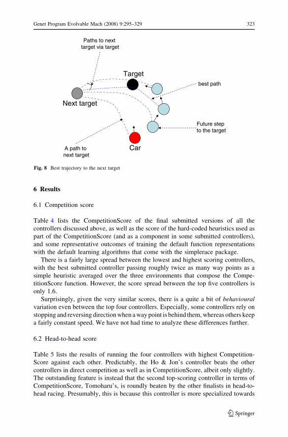
6 Results

6.1 Competition score

Table 4 lists the CompetitionScore of the final submitted versions of all the

controllers discussed above, as well as the score of the hard-coded heuristics used as

part of the CompetitionScore (and as a component in some submitted controllers),

and some representative outcomes of training the default function representations

with the default learning algorithms that come with the simplerace package.

There is a fairly large spread between the lowest and highest scoring controllers,

with the best submitted controller passing roughly twice as many way points as a

simple heuristic averaged over the three environments that compose the Compe-

titionScore function. However, the score spread between the top five controllers is

only 1.6.

Surprisingly, given the very similar scores, there is a quite a bit of behaviouralvariation even between the top four controllers. Especially, some controllers rely on

stopping and reversing direction when a way point is behind them, whereas others keep

a fairly constant speed. We have not had time to analyze these differences further.

6.2 Head-to-head score

Table 5 lists the results of running the four controllers with highest Competition-

Score against each other. Predictably, the Ho & Jon’s controller beats the other

controllers in direct competition as well as in CompetitionScore, albeit only slightly.

The outstanding feature is instead that the second top-scoring controller in terms of

CompetitionScore, Tomoharu’s, is roundly beaten by the other finalists in head-to-

head racing. Presumably, this is because this controller is more specialized towards

Fig. 8 Best trajectory to the next target


123

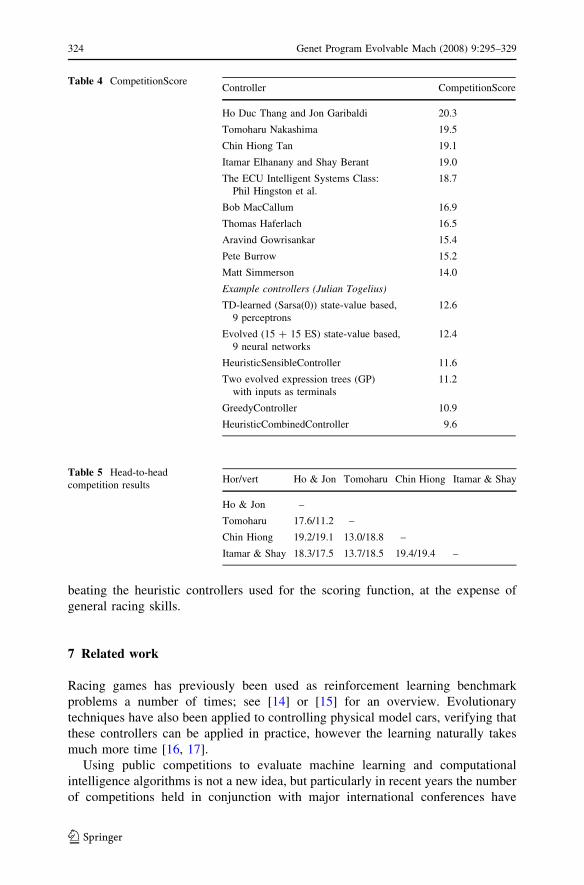
beating the heuristic controllers used for the scoring function, at the expense of

general racing skills.

7 Related work

Racing games has previously been used as reinforcement learning benchmark

problems a number of times; see [14] or [15] for an overview. Evolutionary

techniques have also been applied to controlling physical model cars, verifying that

these controllers can be applied in practice, however the learning naturally takes

much more time [16, 17].

Using public competitions to evaluate machine learning and computational

intelligence algorithms is not a new idea, but particularly in recent years the number

of competitions held in conjunction with major international conferences have

Table 5 Head-to-head

competition resultsHor/vert Ho & Jon Tomoharu Chin Hiong Itamar & Shay

Ho & Jon –

Tomoharu 17.6/11.2 –

Chin Hiong 19.2/19.1 13.0/18.8 –

Itamar & Shay 18.3/17.5 13.7/18.5 19.4/19.4 –

Table 4 CompetitionScoreController CompetitionScore

Ho Duc Thang and Jon Garibaldi 20.3

Tomoharu Nakashima 19.5

Chin Hiong Tan 19.1

Itamar Elhanany and Shay Berant 19.0

The ECU Intelligent Systems Class:

Phil Hingston et al.

18.7

Bob MacCallum 16.9

Thomas Haferlach 16.5

Aravind Gowrisankar 15.4

Pete Burrow 15.2

Matt Simmerson 14.0

Example controllers (Julian Togelius)

TD-learned (Sarsa(0)) state-value based,

9 perceptrons

12.6

Evolved (15 + 15 ES) state-value based,

9 neural networks

12.4

HeuristicSensibleController 11.6

Two evolved expression trees (GP)

with inputs as terminals

11.2

GreedyController 10.9

HeuristicCombinedController 9.6


123

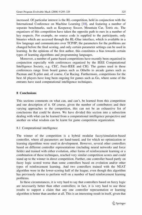
increased. Of particular interest is the RL-competition, held in conjunction with the

International Conference on Machine Learning [18], and featuring a number of

separate benchmarks, such as Keepaway Soccer, Mountain Car, Tetris etc. The

organizers of this competition have taken the opposite path to ours in a number of

key respects. For example, no source code is supplied to the participants, only

binaries which are accessed through the RL-Glue interface, which is available in a

few language and communicates over TCP/IP; the parameters for the problems are

changed before the final scoring, and only certain parameter settings can be used in

learning. In the opinions of the first author, this constitutes a bias towards certain

types of learning algorithms and programming languages.

Moreover, a number of game-based competitions have recently been organized in

conjunction especially with conferences organized by the IEEE Computational

Intelligence Society, e.g. CEC, Fuzz-IEEE and CIG. The games used in these

conferences range from board games such as Othello to arcade games such as

Pacman and X-pilot and, of course, Car Racing. Furthermore, competitions for the

best AI players have long been ongoing for games such as Go, where some of the

entrants have used computational intelligence techniques.

8 Conclusions

This sections comments on what can, and can’t, be learned from this competition

and our description of it. Of course, given the number of contributors and their

varying approaches to the competition, this can not be an exhaustive list of

conclusions that could be drawn. We have divided this section into a subsection

dealing with what can be learned from a computational intelligence perspective and

another on what wisdom can be learnt for game competition organization.

8.1 Computational intelligence

The winner of the competition is a hybrid modular fuzzy/simulation-based

controller, where all parameters are hand-tuned, and for which no optimization or

learning algorithms were used in development. However, several other controllers

based on different controller representations (including neural networks and force

fields) and trained with either evolution, other forms of reinforcement learning or a

combination of these techniques, reached very similar competition scores and could

stand up to the winner in direct competition. Further, one controller based partly on

fuzzy logic scored worse than some controllers based on evolution and/or other

types of reinforcement learning. And two controllers trained with the NEAT

algorithm were in the lower-scoring half of the league, even though this algorithm

has previously shown to perform well on a number of hard reinforcement learning

problems.

In these circumstances, it is very hard to say that controllers based on fuzzy logic

are necessarily better than other controllers; in fact, it is very hard to use these

results to support a claim that any one controller representation or learning

algorithm is better than another at all. This is an interesting result in itself, given that


123

there are people with very strong beliefs about the superiority of one method over

all others, or the total worthlessness of other specific methods. Instead, the most

important factors for the success of a controller seems to have been the familiarity

of the participating team with their algorithm(s) of choice, the amount of time spent

by the team in empirically tuning the algorithm(s) and devising a good training

regime, and to some extent luck.

Still, there are two features which are recurring in most of the better-scoring

controllers and absent in most of the lower-scoring. One of these is modularity. All

the well-performing neural network controllers were composed of different sub-

networks, and most of the other controllers in the top half of the league were

similarly divided into different modules, taking care of the different aspects of the

control task. A popular modularization, representing a clever incorporation of

domain knowledge, is using one module for deciding which way point to aim for

and another to steer the car to the desired way point, but we have also seen e.g. a

module for deciding when to reverse the car. The other recurring feature is internal

simulation of the opponent car, using a model of the opponent controller, to predict

which car will reach the current way point first, a prediction which is then used to

decide which way point to aim for.

Now to the question: how good are these controllers? This is really two

questions: how good are the controllers for racing solo, and how good are they for

two-car competitive racing? For solo racing, the top-scoring controllers are probably

close to optimal. We don’t know of a way of proving this rigorously, but the top

controllers perform very similarly in solo racing, they all outperform good human

players, and visual inspection of their driving behaviour reveals no obvious

mistakes. Competitive racing is another matter. Here, two top controllers can

perform very similarly in solo car racing even though one outperforms the other by a

large margin in a head-to-head race. Further, while no systematic studies have been

made of human and machine controllers head-to-head, there is circumstantial

evidence that a good human player can often ‘‘outsmart’’ even the top controllers,

by learning their driving patterns and way point prediction mechanism, and reach

higher scores. To realiably beat a good human player, a controller would probably

have to incorporate on-line learning of the driving style of this particular competitor.

Thus, it seems that the potential performance gains in head-to-head racing are not at

all exhausted in the simplerace game.

8.2 Competition organization

Given the amount of domain knowledge that was infused into the better-performing

controllers, the reader might get the impression that the competition was more about

clever tricks for hand-coding racing controllers than about learning algorithms.

While such a verdict would be unfair given the prominent use of CI algorithms in all

submissions (it would be more fair to say that the competition was partly about

knowing for which aspects of a problem to use learning algorithms, and for which

aspects to use hand-coding), concern remains about how to make sure that we are

benchmarking learning algorithms rather than programming skills. One suggestion

is to change the fitness function (e.g. which tracks to use, or the car model) between


123

the initial ranking and the final scoring, forcing a degree of generality on the

solution. This could be taken further and allowing the learning algorithm some

further learning time before final evaluation, on the final version of the problem but

without the presence of the experimenter, similar to what is done in the RL-

competition. However, it seems to be very hard to define a framework and interface

for this that is reasonably simple and does not discriminate against particular

learning algorithms. It could also be argued that by allowing controllers to enter the

competition that were not primarily based on learning, we are giving learning

controllers more of a challenge, and assuring that if the winner is based on CI

methods, this means that CI methods are really competitive with other methods in

this domain.

Throughout the organization of this competition, we have strived for simplicity

and transparency. Interfaces were designed to be as simple as possible, software

cross-platform, dependence on external libraries minimal, and all source code made

public as soon as possible. In this way, we succeeded in fostering a decent amount

of participation, though even more participants would of course have been welcome.

(But competitions that fail to attract more than one or two entrants because of how

hard it is to set up the software or understand the interface are not unheard of.) The

competition has also resulted in a repository of good controllers showcasing various

methods of solving the simplerace task, which is undeniably more useful than just a

list of participant names and their respective scores.

One unexpected but very welcome development was the adoption of the

competition task and software for class exercises; the only submitted controller that

was developed this way was the (rather well-performing) one from Phil Hingston’s

Intelligent Systems class, but we know that several other teachers at least considered

using the software and task in a similar way. Of course, the software together with

documentation and submitted controllers is still available on the web page, so there

is nothing hindering teachers from continuing to use the software for these purposes

in the future.

An unexpected problem with the submission and scoring method was that many

of the top-scoring controllers were very computationally expensive to run, due to

the use of opponent modelling. For some controllers, the CompetitionScore can take

hours to calculate on a normal laptop computer. This problem became especially

prominent towards the very end of the competition, when several controllers were

submitted per day, and fast updating of the league table was important. In future

competitions, a cap on computation time taken will have to be used.

Another problem with the submission method was that the winning submission

was the very last controller to be submitted, not giving other participants a chance to

learn from the success of that controller and tune their own controllers accordingly.

A possible effect of this is that participants in the future choose to only submit their

controllers toward the very end of the competition, a development which would be

most unwelcome. This might be counteracted by having two deadlines, one for new

submissions, and another for refinements of these submissions.

One of the aims of this competition was to have representatives for the various

subfields of computational intelligence represented, a goal we think was accom-

plished, given the wide variaty of CI methods used by the different participants. In


123

subsequent competitions in the computational intelligence and games it would be

desirable to have not only computational intelligence researchers, but also people

from outside academia participate. Especially, participation from commercial game

developers could help form bonds between CI research and industry. However, it

seems game developers are rather distrustful of the value of testing algorithms on

games as simple as simplerace. One solution would be to use an open-source game

engine, such as the racing game TORCS, which features more advanced dynamics

and 3D graphics, or the Quake games. However, great care would have to be taken

in order to simplify participation as much as possible. Requiring participants to use

a particular operating system or programming language risks reducing participation

drastically.

While on the sum we feel that the benefits of transparency far outweigh the

disadvantages, one effect of this decision worth pointing out is a fair amount of

‘‘feature diffusion’’. Participants often studied each others’ source code and imitated

features seen to be successful in other controllers, such as using a separate decision

layer for way point choice (pioneered by Pete Burrow), and internal simulation of

the other car for predicting who will reach the next way point first. It is worth

considering only releasing the source code of contributed controllers after the

conclusion of the competition in a future iteration, though Java source code can

always be decompiled (and we must release binaries during the course of the

competition so competitors have good opponent to test their controllers against),

and if a substantially identical version of the game is used for a future competition

the best controllers from the last competition will be around anyway. In the end, as

long as no outright plagiarism goes on (and the publication of the source code would

make such plagiarism easy to detect had it happened) we believe this should be seen

as a beneficial effect, as it leads to better controllers being submitted.

Acknowledgements Thanks to anonymous reviewers for a number of helpful comments.

References

1. M. Monster, Car physics for games. http://home.planet.nl/ monstrous/tutcar.html (2003)

2. D.M. Bourg, in Physics for Game Developers (O’Reilly, 2002)

3. K.O. Stanley, R. Miikkulainen, Competitive coevolution through evolutionary complexification.

J. Artif. Intell. Res. 21, 63–100 (2004)

4. K.O. Stanley, Efficient evolution of neural networks through complexification. PhD thesis, Depart-

ment of Computer Sciences, University of Texas, Austin, TX (2004)

5. J. Togelius, P. Burrow, S.M. Lucas, Multi-population competitive co-evolution of car racing con-

trollers. In Proceedings of the IEEE Congress on Evolutionary Computation (CEC) (IEEE Press,

2007), pp. 4043–4050

6. T. Miconi, A. Channon, The n-strikes-out algorithm: a steady-state algorithm for coevolution. in

Proceedings of the IEEE Congress on Evolutionary Computation (CEC) (IEEE Press, 2006),

pp. 1639–1646

7. F. Gomez, R. Miikkulainen, Incremental evolution of complex general behavior. Adapt. Behav. 5,

317–342 (1997)

8. R.D. Beer, On the dynamics of small continuous-time recurrent neural networks. Adapt. Behav. 3,

471–511 (1995)


123

http://home.planet.nl/ monstrous/tutcar.html

9. F. Gomez, J. Schmidhuber, R. Miikkulainen, Efficient non-linear control through neuroevolution. In

Proceedings of the European Conference on Machine Learning (ECML), ed. by J. Furnkranz,

T. Scheffer, M. Spiliopoulu (2006), pp. 654–662

10. R.M. MacCallum, Introducing a Perl genetic programming system: and can meta-evolution solve the

bloat problem. In Genetic Programming, Proceedings of EuroGP’2003. Volume 2610 of LNCS, 14–

16 April 2003, ed. by C. Ryan, T. Soule, M. Keijzer, E. Tsang, R. Poli, E. Costa (Springer-Verlag,

Essex, 2003), pp. 364–373

11. R.M. MacCallum, The Open Source Perl Genetic Programming System. http://perlgp.org (2003)

12. R.S. Sutton, A.G. Barto, in Reinforcement Learning: An Introduction (MIT Press, Cambridge, MA,

1998)

13. D.T. Ho, J.M. Garibaldi, A novel fuzzy inferencing methodology for simulated car racing. In To bePublished in the Proceedings of the IEEE International Conference on Fuzzy Systems (FUZZ-IEEE)(IEEE Press, 2008)

14. J. Togelius, S.M. Lucas, R. De Nardi, Computational intelligence in racing games. in AdvancedIntelligent Paradigms in Computer Games, ed. by N. Baba, L.C. Jain, H. Handa (Springer, 2007)

15. J. Togelius, Optimization, imitation and innovation: computational intelligence and games. PhD

thesis, Department of Computing and Electronic Systems, University of Essex, Colchester, UK, 2007

16. I. Tanev, M. Joachimczak, H. Hemmi, K. Shimohara, Evolution of the driving styles of anticipatory

agent remotely operating a scaled model of racing car. In Proceedings of the IEEE Congress onEvolutionary Computation (CEC) (IEEE Press, 2005), pp. 1891–1898

17. J. Togelius, R. De Nardi, H. Marques, R. Newcombe, S.M. Lucas, O. Holland, Nonlinear dynamics

modelling for controller evolution. In Proceedings of the Genetic and Evolutionary ComputingConference (GECCO) (ACM Press, London, UK, 2007)

18. S. Whiteson, A. White, R. Sutton, D. Precup, P. Stone, M. Littman, N. Vlassos, M. Riedmiller, Rl

competition. http://rl-competition.org (2008)


123

http://perlgp.org

http://rl-competition.org

the 2007 ieee cec simulated car racing competition

Documents