1

Testing the theories of law making in a parliamentary democracy:

a roll call analysis of the Italian Chamber of Deputies

Luigi Curini & Francesco Zucchini Paper prepared for ECPR joint sessions in Rennes, April 2008

(first draft, do not quote without permission)

Workshop: Comparing legislatures worldwide: roles, functions and performance in old and new democracies (directors: Natalia Ajenjo and Mariana Llanos)

Abstract

The theoretical efforts in the rational choice approach to explain the law making in United States Congress has been increasingly matched by attempts to test comparatively the explicative power of the different theories (Krehbiel et al 2005, Cox & McCubbins 2005). No similar effort has been made by the scholars studying the parliamentary democracies. In this paper we try to start filling this gap. Using roll calls of the 10th, 13th and 14th Italian legislatures we try to test via cut points distribution the explicative power in a parliamentary system of some of the law making theories. We aim to evaluate their explicative strength according to the dynamics of the party system, the type of government and the nature of the bill’s promoter. Introduction The theoretical efforts in the rational choice approach to explain the law making in United States

Congress has been increasingly matched by attempts to test comparatively the explicative power of

the different theories (Krehbiel et al 2005, Cox & McCubbins 2005). No similar effort has been

made by the scholars studying the parliamentary democracies1. Strictly intertwined reasons can

explain such a gap. “Positive” explanations of the law making in the Parliamentary democracies are

recent and did not trigger yet the same sanguine debate that enlivens the scientific community of the

Congress’ scholars. Besides, given the centrality of the Cabinet in the Parliamentary systems, most

of the theoretical and empirical efforts have been absorbed by the studies of the government

formation and dissolution. Such a prevalent scientific focus has induced to collect data very useful

for testing coalition theories, as for instance the expert survey data (Laver & Hunt 1992 , Laver &

Schofield 1991), but it has also induced to disregard the collection of other data, as the roll calls

data, that were evidently useless for testing government formation models , even if potentially

useful for other research goals.

In this paper we try to start filling this gap. Using roll calls of the 10th, 13th and 14th Italian

legislatures, differentiable also according to the nature of the legislative promoter (cabinet versus

Mps), we try to test the explicative power in a parliamentary system of some of the law making

1 A partial exception is represented by the papers published in the Cox & McCubbins website www.settingtheagenda.com .

2

theories. The choice of more than one legislature is not only driven by the trivial need to increase

the number of cases. The 10th Legislature can be considered the last long legislature of the Italian

first republic, namely a legislature characterized by a pivotal party system without perspective of

government alternation. On the contrary the other legislatures belong to the second republic and

they were characterized by two subsequent government alternations. Moreover in the 13°

Parliament, a minority government is followed by barely minimum winning cabinets while during

the 10th and 14th legislature most of the government are oversized.

Therefore we aim to evaluate the explicative strength of each law making model according to:

a) the dynamics of the party system; b) the type of government; c) the nature of the bill’s promoter.

In the next section we illustrate a typology of law making models based upon the distribution of

veto power inside the government and the government’s agenda setting power vis a vis the

parliament. In the following sections we explain the cut points method to assess the empirical

support of each model and the roll call analysis used to create the legislative space. After a

discussion of the conceptual problems connected to the dimensions and to the ideal points inferred

from the roll call analysis, the Italian legislative space for the each period is presented and

commented . In the last two sections we show the results of our test and discuss the broadest

implications.

Theories of law making in the parliamentary democracies. In the recent developments of the positive theory of America Congress two competing theoretical

models of law making seem to be survived by the scrutiny of the empirical research: the so called

pivotal politics model and the party cartel model (Krehbiel 2006).

In the first one Krehbiel contends the either of two agents- a veto pivot or a filibuster pivot- can

prevent any change of the status quo if such a change produces a final outcome worse for him/her

than the initial status quo. The nature and the identity of this two actors are determined by 1) the

qualified majority required by the standing orders and practices that rule the activity in the Senate

(filibustering) and the interaction between the Congress and the President (veto overriding ) 2) by

the position of the political actor in the legislative unidimensional space.

In the party cartel model Cox and McCubbins (Cox & McCubbins 2005) contend that the majority

party leadership, located in party median position, can prevent any change of the status quo that the

majority of the majority party dislikes. Both theories insist on the negative powers of some political

actors but they differ substantially on the identity of these political actors and on their role when

the veto is not put.

3

In the party cartel model once the party leadership has “opened the gate”, it cannot prevent the

parliament from legislating according to the floor median desires. On the contrary in the pivotal

politics model the last word is given to the pivotal actors (if the median voter is the first mover ). If

a change is considered positively by both pivots, then the final outcome will be the nearest

alternative to the floor median voter, among the alternatives the pivot nearest to the status quo still

considers an improvement. If the status quo is “far enough”, both models will predict the floor

median position as final outcome. Otherwise the predictions will differ.

Both models cannot be immediately and unconditionally transferred to a parliamentary democracy.

Cartel party model can be directly applied only to a one party government. When there is a

government coalition the model is open to different adaptations. Government coalition can be

considered as a party . In this case only the government median party exercises the veto power (we

will call such adaptation “government median party” model). Alternatively any government party

can have the power to veto a change of the status quo ( (we will call such adaptation “all

government parties model”). In this last case2 the veto power derives from the possibility for each

government party to risk the government’s and eventually the legislature’s life.

The pivotal politics model depends crucially on the special majorities of the US system. Therefore it

seems even more hardly exportable than the cartel party model. However in the comparative

politics literature one of the most successful model of law making in the parliamentary

democracies, the Tsebelis’s veto player model (Tsebelis 2002) , shares a crucial analytical property

with the Krehbiel’s model: the government parties in the parliamentary systems as the pivots in the

Congress have “practically” the last word, at least insofar we do not consider the minority

government. When the policy change is a Pareto improvement for all government party leaders, the

government party leaders find an agreement and bind their backbenchers to this agreement during

their following floor behaviour, preventing, if necessary, the floor median voter’s outcome. Such a

result can be obtained in two ways, not necessarily mutually in contrast: government party leaders

agree not only on the legislative content but also on presenting the bill in front of the parliament

with a closed rule (take or leave it offer) that prevents the parliament from emending the

government proposal; government party leaders can take advantage of a rigid party discipline. The

only plausible (and empirical) difference between the two ways to protect the government’s

proposals is that in the first case, with only the closed rule, we should observe more often

government party members voting against the government.

In order to clarify and summarize the possible law making models of the parliamentary

democracies, explicitly proposed by the authors or that we can reasonably infer from the rational 2 This last adaptation seems to be the version of the procedural cartel theory proposed by Cox, Heller and MCubbins in application of the model to the Italian case. (Cox, Heller & McCubbins 2008)

4

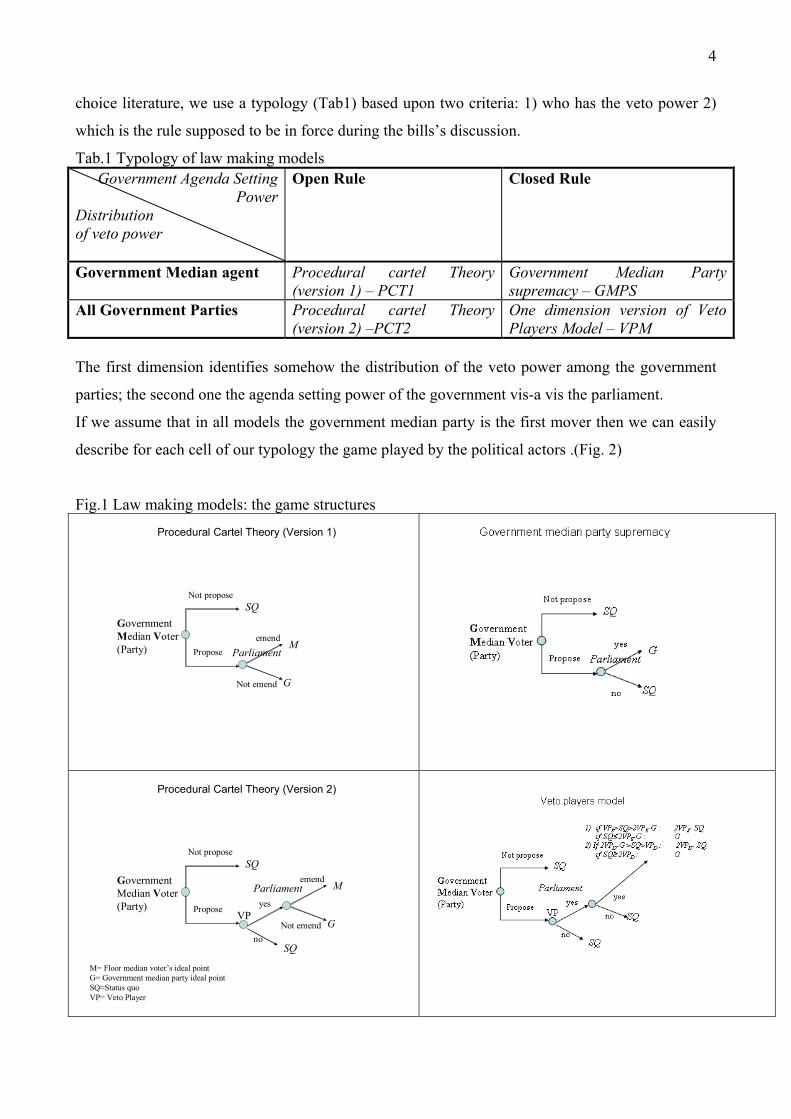
choice literature, we use a typology (Tab1) based upon two criteria: 1) who has the veto power 2)

which is the rule supposed to be in force during the bills’s discussion.

Tab.1 Typology of law making models Government Agenda Setting

Power Distribution of veto power

Open Rule Closed Rule

Government Median agent Procedural cartel Theory (version 1) – PCT1

Government Median Party supremacy – GMPS

All Government Parties Procedural cartel Theory (version 2) –PCT2

One dimension version of Veto Players Model – VPM

The first dimension identifies somehow the distribution of the veto power among the government

parties; the second one the agenda setting power of the government vis-a vis the parliament.

If we assume that in all models the government median party is the first mover then we can easily

describe for each cell of our typology the game played by the political actors .(Fig. 2)

Fig.1 Law making models: the game structures

Propose

Not proposeSQ

GovernmentMedian Voter (Party) Parliament

emend

Not emend G

M

Procedural Cartel Theory (Version 1)

Propose

Not proposeSQ

GovernmentMedian Voter (Party)

VP

noSQ

Parliamentyes

emend

Not emend G

M

Procedural Cartel Theory (Version 2)

M= Floor median voter’s ideal pointG= Government median party ideal pointSQ=Status quoVP= Veto Player

5

In a one dimension world each model helps to identify both a non decision line (gridlock) and the

legislative outcome when the legislative decision is possible. In the following graphs (Fig.2) the

solid lines describe the outcome location in one dimension for all possible positions of the status

quo in horizontal axis. When the outcome replicates perfectly the original status quo then there is no

legislative change. This circumstance takes place when the status quo’s change should imply a

worsening for at least a one crucial actor who according the legislative game can prevent it. For

instance with respect to the model PCT2 the two extreme government parties VPS and VPD cannot

agree to change a status quo when the status quo fall in the interval (2VPS- M) – (2VPD- M). These

point are respectively spaced at the same distance from VPS and from VPM as M. As according to

this model the government does not enjoy a strong agenda setting power, once proposed a bill to

parliamentary floor, the final outcome will be M. When SQ is in the interval (2VPS- M) – (2VPD-

M) it is better for both crucial actors than M. Such an example shows quite well that the extension

of the “gridlock line” depends on two features: the distance between the two most distant “crucial”

actors (in this example the VP actors) and the location of the final outcome in the policy dimension

when the veto is not put. This feature depends, on its turn, on the government agenda setting power.

If the Governments with the same crucial actors enjoy different level of agenda setting power vis a

vis the parliament then also the gridlock line will differ: a weak agenda setting power, (i.e. open

rule) as hypothesized in the procedural cartel theory, will imply more policy stability and a longer

gridlock line. On the contrary the closed rule (and/or a rigid party discipline in the case of the Veto

Player Model) should increase the probability of the legislative change.

6

Fig. 2 Law making models: legislative space, outcomes and cut points distribution Outcomesand “no cut points area”

Status quoM

(parliament’s median voter)

G (governent’smedian voter)

G

I II III

VPS VPD

M

Procedural cartel theory (version 1)

outcomes

cut points

2G-M

VPD

VPS

No cut points area

Gridlock

Outcomesand “no cut points area”

Status quoM

(parliament’s median voter)

G (governent’smedian voter)

G

I II III

VPS VPD

M

Government median party supremacy

outcomes

cut points

2G-M

VPD

VPS

No cut points area

Gridlock

2M-G

Outcomesand “cut points”

Status quoM(parliament’s median voter)

G(governent’smedian voter)

G

I II III

VPS VPD

M

Procedural cartel theory (Version 2)

outcomes

cut points

2 VPD -M2 VPS -M

VPD

VPS

Gridlock

No cut points area

Outcomesand “no cut points area”

Status quoM

(parliament’s median voter)

G (governent’smedian voter)

G

I II III

VPS VPD

M

Veto players model

outcomes

cut points

2 VPD -G2 VPS -G2G-M

VPS

VPD

Gridlock

No cut points area

Is it possible to test which of the previous model describes better the legislative process in the

Italian Parliament ? Is the explicative power of the models conditioned to some other characteristic

of the political system as the party system dynamic or the government coalition size? The

exploratory analysis of the roll calls (final voting ) in the Italian Chamber of Deputies that we are

going to present should help us give some preliminary answers. However the gulf separating the

spatial models just illustrated and the empirical data on roll calls is large enough to require some

further cautious methodological investigations.

In the horizontal axis of all models the change of the status quo along the policy dimension creates

different legislative outcome. Therefore if we knew the position of the status quo for each policy

issues we could compare the position of the bill as predicted by each model with the position of the

bill as inferred by the data analysis; then we could identify the model fitting better the empirical

observation. Unfortunately no statistical method using roll call data allows to identify a reliable

position of the approved bill. In the next paragraph we will deal with this problem. In the following

7

ones after having explained the feature of the main methods used to infer from the final voting

behaviour the legislative space, we will show the Italian legislative space and its parties and we will

discuss its origin and meaning.

Status quo and cut points. A roll call data analysis does not allow to know reliable positions in the legislative space of the

approved bills (or to be more precise the position of the legislative outcome). However it generates

another measure that can indirectly help us to test the different models. Such a measure is the cut

point. The cut point is a roll call specific midpoint between the estimated bill and the status quo

location( Krehbiel and alt. 2005). Consider the case of a vote on final passage of a bill b. In this

voting b is implicitly paired against the status quo sq. If the legislators have symmetric single

peaked preferences, then the cut point for such a vote is c=(b+sq)/2. Therefore the same analytical

model that predicts for all possible status quo a certain distribution of the legislative outcomes,

predicts also a certain distribution of cut points. As this last estimates are made available by some

methods for analyzing the roll calls (the family of methods called Nominate) , we can test indirectly

the models previously presented.

Imagine that we want to test the version 1 of procedural cartel theory – PCT1–- (Fig.3)

Any legislative change when the status quo SQ is in the range (M)-(2G-M) will be vetoed: the final

outcome would be M and the status quo SQ is for G better than M. On the contrary, when the status

quo is for instance SQ1, G should welcome any legislative change, given that M for G is now better

than SQ1. What about the locations of the cutpoints? In the first case, by definition, we expect to

find no cutpoint in the data. In the second case, a cutpoint must be found between G and 2G-M (if

the status quo is SQ it will be “cut”). As a result, by looking at the partition of the policy space in

which, according to PCT(1), we do not expect to find any cutpoints (i.e., between M and G), we

have a way to test the validity of the theory. It is worth noting that in this case the gridlock line is

longer than the “no cut point line”. The same happens with PCT(2) but not with the other two

theories (in which the two lines perfectly overlap).

Fig.3

8

The models of our typology that share the same distribution of veto power (PCT1 and GMPS versus

PCT2 and VPM) share also the same “no cut” line. However , as it is pretty clear looking at the

figures (Fig.2 ), the expected distributions of the cut points on the whole legislative space are quite

different from one model to the other even when the “no cut points line” is the same.

Therefore the cut points analysis helps to adjudicate among the lawmaking models of our typology

in two steps : first we look at the presence/absence of the cut points inside the “no cut line” in order

to evaluate which of the two groups/sets of models (PCT1 and GMPS versus PCT2 and VMP) fits

the data better. Secondly we observe the distribution of the cut points near the crucial actors of the

group of models that has fared better in the previous selection’s stage. In the case of the “All

Government Parties” models, if the VMP fits better the data than PCT2, we should find a

remarkable density of cut points around the position of VPs and VPd. Similarly, in the case of the

Government Median agent, if the Government median party supremacy model (GMPS) fits better

the data than PCT1, we should find many cut points concentrated around M .

The methods to analyze the roll calls. There are two general class of statistical model for analyzing the roll calls: parametric and non-

parametric ones (Poole 2005). The former recover metric information about legislator and roll-call

characteristics (in particular, for our purpose, the cut points) by assuming that roll-call voting fits a

probabilistic spatial model of voting. Essentially, this approach assumes a spatial model of party

competition in which differences between the policy positions of legislators can be represented as

Euclidean distances. Conditional on these assumptions, the spatial policy positions of legislators are

retrieved by analyzing roll call voting records, treating a pair of legislators with more similar voting

records as being closer to each other than a pair of legislators with less similar records. In particular,

the likelihood of a legislator accepting a proposal depends on the distance of the legislator’s ideal

point from the outcome point for accepting the proposal. The vote is only more likely, not certain,

because the votes are subject to error. Parametric methods differ in their choice of both the

deterministic component of the utility function of the MPs (quadratic or Gaussian) and of the

stochastic components (normal, logit, linear). Still their ability to obtain precise parameter estimates

depends heavily on the errors being relatively substantial.

The non-parametric model (essentially the optimal classification model – OC - developed by Poole

(Poole 2005) does not rely on distributional assumptions about errors to uncover metric information

from binary roll-call data. Instead, OC method derives ideal points by minimising classification

errors. A classification error for a legislator on a roll call occurs when the legislator’s ideal point is

such that his vote is inconsistent with the separating hyperplane for the roll call. This procedure is

9

highly robust to the stochastic nature of the data. Precisely for this reason it has been argued (Vogen

and Rosenthal 2004) that OC is a superior method than its parametric counterparts to analyze roll-

call data in a parliamentary context. In particular, in a legislative setting we can find different

situations (variation in discipline across parties, unstable party memberships, proxy voting,

parliamentary institutions that provide incentives for strategic voting) that may make the

assumptions about errors in voting that underlie the parametric methods not holding anymore. On

the contrary, OC can still produce reliable ideal point estimates in environments where voting errors

are not independent or evenly distributed across legislators and votes.

There is, of course, a price to be paid for using the non-parametric method. Using a non-parametric

method means that OC recovers a rank-order of actors’ ideal points rather than actors’ relative

spatial locations. This problem is particularly serious in one-dimension. If in two or more

dimensions OC can still recover metric information (altough in a different way compared to a

parametric model), in one-dimension we can recover only a rank order of legislator ideal points

(and roll-call cutting points). Two adjacent legislators in the rank order might have, in other words,

ideal points that are very close or very distant.

Given that the lawmaking theories we are going to test assume a unidimensional policy space, we

cannot rely on OC to analyze our roll-call data. Instead, we will employ the W-Nominate algorithm.

However, as we recognize the possible risks associated with a parametric model, we will use OC to

check the reliability of our results.

The W-Nominate algorithm estimates the positions of legislator ideal points as well as roll-call cut

points (i.e. the point in one dimension or line in two dimensions that divides the legislators

predicted by the model to favour a proposal from those expected to vote against it) such that the

likelihood assigned to each observed vote is maximized. The estimated ideal point of a MPS should

be seen in this framework as the point that best represents a legislator’s position in the Chamber of

Deputies relative to other legislators. The higher the probability with which the model predicts

correctly the MP’s voting choice, the better the model fits the data.

Building the space and mapping the parties: W-Nominate data analysis Following Poole and Rosenthal (1997) only roll calls with at least 2.5 percent in the minority are

included in the computations. We have excluded also MPs with fewer than 25 votes. Besides, we

focus on final passage votes only. Our assumption here is that voting decisions on successful final

passage votes should reflect (in a more accurate way) policy preferences (than, let’s say, procedural

or amendments votes), and so they should present the closest connection to the lawmaking theories.

10

It is worth noting that W-Nominate (as well as OC) allows only dichotomous behaviour: yes and

nay. On the contrary, the real voting includes at least two other choices that according the

circumstances and the institutional rules can be equivalent to (or nearer to) yes or nay: Absence and

Abstention. According to the rules in the Italian Lower House all the Mps who abstain are counted

for the quorum necessary to make valid the vote, but they are not counted to establish the majority

of votes necessary to win. Therefore, abstentions cannot be counted as nays but on the contrary they

have to be counted as yes. For the same reason in some circumstances being absent has a “negative”

valence. In particular, when a coalition of parliamentary groups try to boycott the voting by

preventing the quorum that makes valid the vote or when a group wants to signal in front of the

public opinion its complete refusal of the bill. Both behaviours require collective coordination and

group discipline. Therefore absence of an MP can be considered nay when almost all members of

his/her parliamentary group are absent. Otherwise it is considered as a missing value.

Finally, the present analysis is based mainly upon the assumption that each MP belongs to the

parliamentary group of the last parliamentary session, while holding constant his/her ideal point

during the whole legislature regardless of any party switching (for example, we consider a MP that

originally started as a member of FI before joining later to UDC, as having a fixed ideal point

throughout the Legislature. Moreover, we take into account this ideal point to estimate the median

position of UDC – not of FI)3. The only exceptions made to this rule concern the MPs belonging to

parties that during a Legislature switched from being government’s members (or at least

supporters,) to be an opposition party. In this case the parties are labelled with different names

according to their relationship with the government, and their median point is calculated for each

different label as if the legislature was characterized by more than one party only officially with the

same name. This applies to Pri in the 10th legislature and to RC and UDEUR in the 13th legislature.

As it will be show more clearly below, this distinction matters when assessing the ideal points of

the MPs.

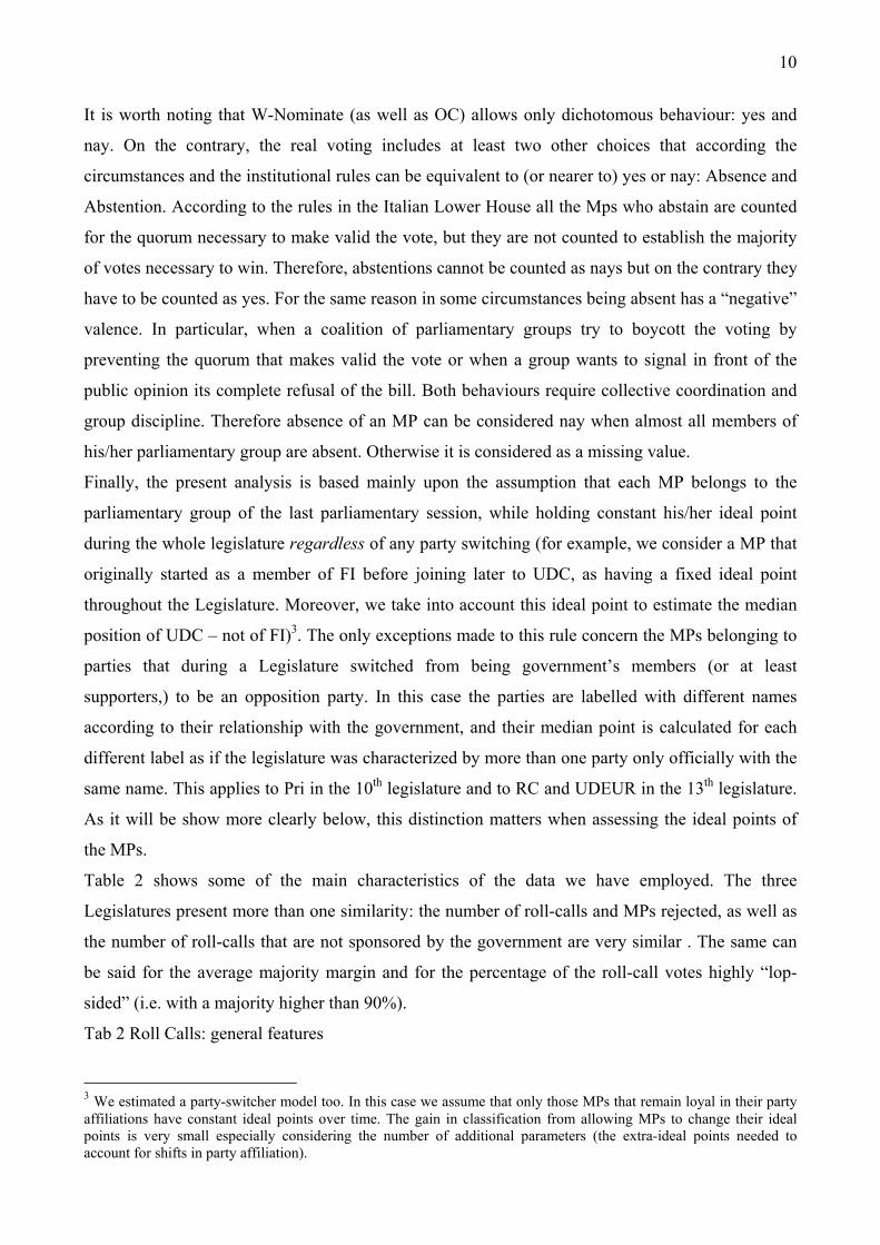
Table 2 shows some of the main characteristics of the data we have employed. The three

Legislatures present more than one similarity: the number of roll-calls and MPs rejected, as well as

the number of roll-calls that are not sponsored by the government are very similar . The same can

be said for the average majority margin and for the percentage of the roll-call votes highly “lop-

sided” (i.e. with a majority higher than 90%).

Tab 2 Roll Calls: general features 3 We estimated a party-switcher model too. In this case we assume that only those MPs that remain loyal in their party affiliations have constant ideal points over time. The gain in classification from allowing MPs to change their ideal points is very small especially considering the number of additional parameters (the extra-ideal points needed to account for shifts in party affiliation).

11

Roll calls read

Roll calls parl. origins

(% tot.)

Roll calls accepted

(cutoff=0.025)

% Roll call

rejectedMPs read

MPs accepted

(cutoff=25)% MPs rejected

Average majority margin

% lop-sided roll calls

(>90%)10th legislature (88-92) 413 9.4% 168 59.3% 691 649 6.1% 72.90% 29.20%13th legislature (96-01) 672 11.9% 276 58.9% 708 693 2.1% 78.10% 29.30%14th legislature (01-06) 589 10.2% 252 57.2% 643 607 5.6% 72.50% 32.50%

Table 3 summarizes the overall fit of the spatial models as estimated by W-nominate. As summary

statistics, we present the classification percentages as well as the Average Proportion Reduction in

Error (APRE). The APRE denotes the extent to which the spatial model better accounts for

observed vote choices than a model that simply predicts that each deputy always votes with the

majority on each roll call4.

The uni-dimensionanl space fitted by W-Nominate correctly classified at least 95% of the votes.

The APRE is remarkable as well, with the only partial exception of the 13th Legislature (where it

still reaches almost 80%). Fitting a second dimension resulted in an improvement in classification

accuracy of less than 1% in each legislature. While we do not reject in theory the presence of

multidimensionality in the data, still voting behaviour in thr 10th , 13th and 14th legislatures can be

largely accounted for by a single policy dimensions5. This is of course a good news for applying

and testing our models that imply a unidimensional world.

Table 3: Goodness of fit of the roll call analysis: WNominate and Optimal classification

1dw 2dw 1 oc 2 oc Class % APRE Class % APRE Class % APRE Class % APRE 10th legislature (88-92) 97.7 91.6 98.5 94.3 98.6 94.9 99.3 97.5 13th legislature (96-01) 95.1 77.6 96.6 84.6 96.7 84.7 98.1 91.3 14th legislature (01-06) 97.7 91.5 97.5 90.8 98.6 94.8 99.0 96.2 As previously stressed, when the assumptions about errors in voting that underlie the parametric

methods do not hold, this can jeopardize the validity of the ideal point estimates. In this sense OC is

an important check on all probabilistic methods, given that being built directly on the geometry, OC

is not subject to the vagaries of the error. Therefore we also estimated a 2-dimensional OC and we

compared the ideal points estimation we get along the first dimension (using a 2-dimensional OC) 4 APRE varies from zero to one. When APRE is equal to zero, the model is explaining nothing. When APRE is equal to one, perfect classification has been achieved. 5 Even tough we found a single dominant dimension of political contestation, this does not imply that the world is in some strict sense unidimensional. It can be that the “real world” is composed of many individual issue dimensions that exhibit significant inter-issues constraints, producing the appearance of (and, for predictive purposes, the reality of) a single dimension. As we will see later, the presence of a cabinet is one, if not the main reason, behind this unidimensionality.

12

with the ideal points estimation that result from the unidimensional W-Nominate analysis (a

procedure also suggested in Poole 2005). The correlations are quite high when we compare the MPs

ideal points (average R-Pearson: .9; average Rho: .9) as well as the median parties’ positions

(average R-Pearson: .94; average Rho: .97). We can infer from these tests that even if there are

some violations on the assumptions about errors in voting model, still they are not so huge to

invalidate our findings6.

Figure 4: Median positions and box plots of the main Italian parties

6 Another possible problem of using W-Nominate, instead of OC, is the following. W-Nominate estimates legislator ideal points within a hypersphere of radius one. (In one dimension within an interval from –1 to +1). These constraints, however, pose a problem for probabilistic models as the level of the error in the data decreases (after all, probability assumes the presence of random errors). The corrected classification in our estimations (see Table 2) is very high, so this is risk not far-from-reality in our data. When this happens W-Nominate produces spatial maps with large numbers of legislators at the edges of the space (i.e., close to the two extremes of –1 and +1). For example, Rosenthal and Voegen (2004) found that using a 2-dimensions W-Nominate in the case of the France Fourth-Republic produce one-third of MPs placed at the edges. In our case, the results are however much more favourable: just 2.5% MPs presents a value higher than .98 (considering the three legislatures together); 4.9% higher than .90 (in both cases the 14th legislature present the two highest values: 4.3% and 6.3% respectively).

13

After having estimated the spatial locations of each MPs we estimated also the median positions of

parties (implicitely we consider the median member’s decisions as reflecting the party’s position7).

Figure 4 summarizes both results by legislature using a box plot. Two manifest features of the

graphs deserve a more in-depth comment: 1) the apparent change in the level of dispersion of the

government parties in the passage from the first republic (10th Legislature) to the second republic

(13th and 14th Legislature) 2) the unexpected location of some parties on the legislative space.

We will deal with the first point in the rest of the current section while the next section will be

entirely dedicated to the second one .

At first glance the inspection of the box plots seems to indicate a level of dispersion around the

median much higher for the government parties of the 10th legislature than for the government

parties of the other legislatures. As we know much dispersion should mean lack of party cohesion

and discipline. Once confirmed, a decrease of the dispersion around the median of the government

parties could be an interesting phenomenon to associate both with the change from a pivotal non

competitive party system (10th legislature) to a alternational and competitive one. However the box

plots do not allow to weight such a dispersion according to the relative importance of the party.

Moreover we could be also interested to calculate the level of the overall government cohesion and

discipline at individual level.

We calculate the weighted (according to the importance in seats) mean of the MAD (the median

absolute deviation8) for each government party. We call this measure: “party cohesion in the

government” . Then we calculate also the MAD of the positions of MPs belonging to the

government parties. We call this measure “Government MP’s cohesion”. The first measure tell us

how disciplined and cohesive is on average a government party, regardless if such a party is more or

less loyal to the government; the second one tell us how disciplined and cohesive are the Mps

“belonging” to the government regardless their specific party affiliation.

7 By estimating the MPs ideal points and using them to find the position of a party, we do not treat the party as a unitary actor. On the contrary, we allow the possibility that any divergence in the votings patterns of its members, as well as the degree and the systematic nature of this divergence, affects the estimation of party’s position. Cox, Heller and McCubbins (2008) use a different strategy in their study of the Italian case: first they consider a party to have voted Yea or Nay to a given bill if the majority of its members voted Year or Nay to it. Secondly, they apply a roll-call analysis similar to the one we employed here directly to parties’ voting patterns, instead than to MPs’. So doing , however, they run the risk to underestimate any possible conflict – even if marginally – within a given party. This is a typical ecologic fallacy problem. 8 In statistics, the median absolute deviation (or "MAD") is a resistant measure of the variability of a univariate sample.For a univariate data set X1, X2, ..., Xn, the MAD is defined as MAD=mediani ( |Xj – medianj| ) that is, starting with the residuals (deviations) from the data's median, the MAD is the median of their absolute values.

14

Tab.4 Measures of cohesion Leg. Periods Government MP’s cohesion Party cohesion in government

Pentapartito 0.097 0.058 10th Leg. Quadripartito 0.092 0.051 Prodi Cabinet considered with RC 0.027 0.028 Prodi Cabinet considered without RC

0.023 0.024 13th Leg.

Post Prodi Cabinet 0.026 0.028 14th Leg. Berlusconi Cabinets 0.025 0.015 We have considered the Prodi government (see below) as it was formally (without RC) and adding

also RC, the extreme leftist party that supported the government in the Parliament (see below).

The impressions of the visual inspection are completely confirmed by our measures: both the party

cohesion in the government and the government MP’s cohesion have been increased in the passage

from the first to the second Republic. During the Berlusconi Cabinet the government MP’s cohesion

and the Party cohesion in government were around 26% of the same measures during the

Pentapartito government. We suspect that this change in the voting behaviour is associated with the

change in the party system dynamics: the government alternation and the possibility of government

alternation could have made less divisive and controversial the law making process for the

government parties and the government as whole.

The quandaries of the legislative space Looking at the box plot graphs (Fig. 4) , the one-dimensional spaces resulting from the roll call

analysis seem to well capture the overall ideological position of the government (centre-right in the

10th and 14th legislature, centre-left in the 13th). Still they are in some instances (notably for the 10th

and 13th Legislature) remarkably different from the conventional wisdom and the expert survey data

about Italian Politics during the First and Second Republic . In particular, the position of the neo-

fascist MSI in the 10th Legislature, on the left of the government’s parties, and the position close to

the centre-right parties of the communists (RC-PRO post) in the 13th, after they chose to withdraw

their support to the government. What’s wrong with these results ? Is the conventional wisdom (and

expert survey evaluation) erroneous ?

The previous results should not be a surprise. Indeed, by scaling roll-calls we directly measure the

structure of the “revealed behavioural space”. However, the “dimension” revealed by the voting

behaviour in the parliament is only indirectly linked with the underlying ideological dimension of

conflict in a polity. The difference between an “exogenous preference space” and the “revealed

behavioural space”, as measured by scaling recorded votes in a parliament, can derive from two

factors: the government gatekeeping power (and the fact that in a parliamentary system the vast

15

majority of all legislation, is proposed by the government) (see Table 1); the strategic or

instrumental nature of the opposition voting behaviour in a parliamentary setting.

Let’s start with the first factor. All the models we are going to test hypothesize that some

government actors (all or just the median one) enjoy a de facto gatekeeping power. If these models

are correct from this point of view, the proposals that actually reach the floor will be the proposals

less controversial for the government actors (all or some), namely the ones less risky to divide

government’s parties. Such a circumstance affects the legislative space in three ways :

1) the ideal points recovered through the analysis of the roll-calls become a function of

legislator policy preferences expressed on only those proposals allowed/sponsored by the

actor (the government) who controls the agenda. Of course, there is no requirement that the

substantive topics that are brought to the floor belong to the same policy dimension or hang

together in some logical sense.

2) all voting should be characterized by a pretty homogenous actor (the government party

members ) who has being voted consistently “yes” for the whole government duration, while

the other parties sometime will vote as the government parties and sometimes against the

government parties. This scenario allows to only one dimension to explain very well the

roll-call patterns (in the sense that conventional goodness-of-fit is already maximized by one

dimension). Cabinet existence, in other words, induces one-dimensionality in the legislative

space resulting from roll call analysis, even if the preference’s space behind (and before) can

be multidimensional.

3) As side effect of the government’s gatekeeping power we expect that the government actors

who exercise such a power appear also spatially close each to other.

A second and even more relevant factor differentiates the “exogenous preference space” and the

“revealed behavioural space”. The opposition parties, namely the parties that voted against the

government formation, may pay a price in terms of reputation and reliability towards their

electorate if they vote for a proposal supported also by the government parties. So they have always

to balance the policy effect of any bill with the effect of their voting behaviour on their reputation.

If the government parties are cohesive enough to allow a proposal to pass (and the government is

not a minority government), paradoxically the opposition parties could find very convenient to vote

against the same proposal even when they evaluate it an improvement of the current status quo.

They will win such an improvement preserving at the same time their reputation as opposition

parties. The frequency of this behaviour is very changeable. It depends for each single bill, on

16

which aspect of the voting will prevail in the party communication strategy (and consequently in the

party utility function): the policy content of the bill or the political identity of its supporters.

During the 13th legislature the extreme leftist Rc experienced a movement along the legislative

space that illustrates very well this phenomenon (see Fig ). Once Rc had withdrawn its support to

Prodi’s government , it became firmly placed among the centre-right parties. It is implausible that

suddenly most of the proposals coming from the centre-left governments disfavoured Rc and at the

same time the other centre-right parties (i.e., proposals to which, for example, both Rc and Fi should

vote Nay). Therefore the Rc position can be explained only if we assume that the policy content of

the proposals were not the only criteria behind its voting behaviour.

Summing up, the ideal points coming from a roll call analysis in a Parliamentary setting should be

carefully considered and the legislative space should be not confused or improperly compared with

the political spaces produced by other procedures as the expert survey or the party manifestos data.

Generally what we can say is that we can recover from the analysis at least the sincere preferences

of the government’s parties, in the sense that they will never vote for a change of the status quo that

leaves them worst in terms of policy preferences. In this case we suspect that the sincere

preferences are mostly detected in relation to the proposals actually sponsored or allowed by the

government9. Regarding the opposition parties the situation is much more confused as their

behaviour reflects not only their evaluation in terms of the policy preferences but also the

consequences of their voting behaviour on their image as opposition parties.

At the end of this discussion, the reader could start doubting the utility of roll-calls to test the law

making theories in a parliamentary setting. We believe that such a diffidence would be misplaced.

The common ingredients of all models are the following ones: 1) the distance in one dimension

between the crucial actors of the government matters and it is based upon sincere preferences; 2)

whoever are these crucial actors, they anticipate the final outcome of the decisional process for any

alternative move described in the specific legislative game.

If the distance inferred from the voting behaviour is not calculated de facto on all political issues

but only on the issues that the same actors agree to consider in the government pact, it means that

the same actors consider the other issues less important than the government agreement. Far from

being a “false” distance based upon insincere preferences, such a distance can be considered even

more accurate as it weights indirectly the real salience of the different issues for the government

actors.

9 On the perils of treating the roll-call analysis as exogenous without paying careful attention to how rules, strategies and agenda control shape the roll-call record see Roberts 2007.

17

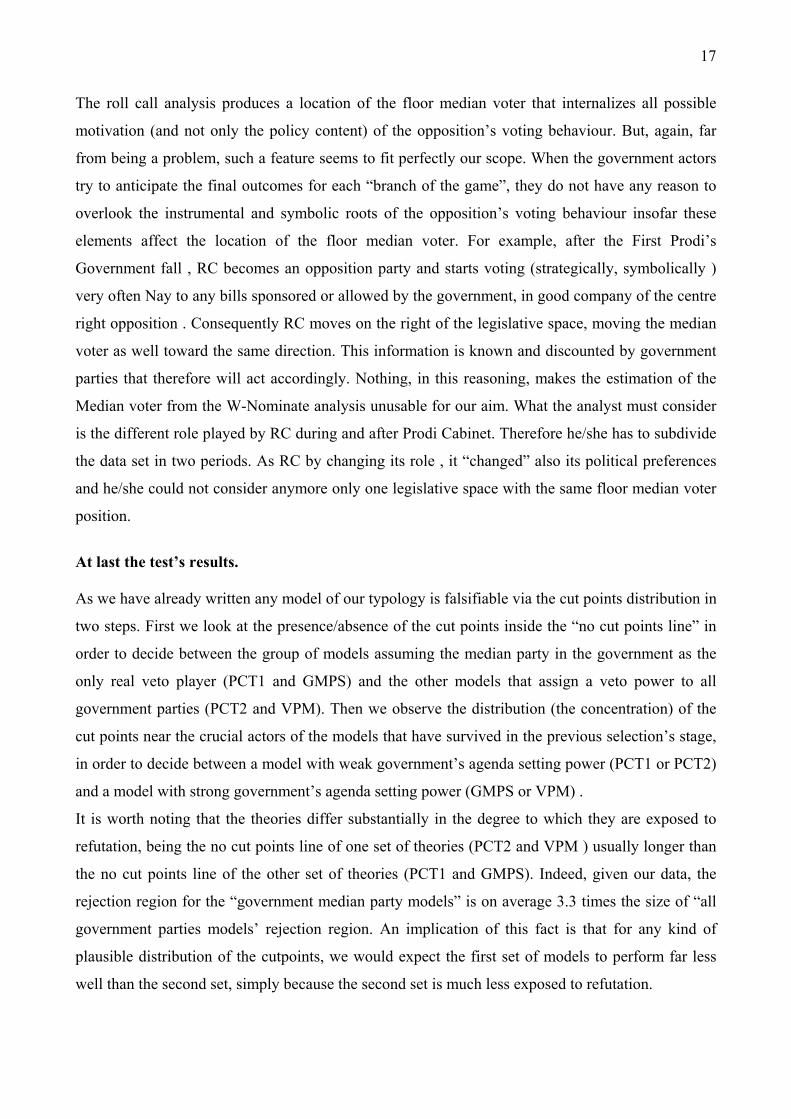
The roll call analysis produces a location of the floor median voter that internalizes all possible

motivation (and not only the policy content) of the opposition’s voting behaviour. But, again, far

from being a problem, such a feature seems to fit perfectly our scope. When the government actors

try to anticipate the final outcomes for each “branch of the game”, they do not have any reason to

overlook the instrumental and symbolic roots of the opposition’s voting behaviour insofar these

elements affect the location of the floor median voter. For example, after the First Prodi’s

Government fall , RC becomes an opposition party and starts voting (strategically, symbolically )

very often Nay to any bills sponsored or allowed by the government, in good company of the centre

right opposition . Consequently RC moves on the right of the legislative space, moving the median

voter as well toward the same direction. This information is known and discounted by government

parties that therefore will act accordingly. Nothing, in this reasoning, makes the estimation of the

Median voter from the W-Nominate analysis unusable for our aim. What the analyst must consider

is the different role played by RC during and after Prodi Cabinet. Therefore he/she has to subdivide

the data set in two periods. As RC by changing its role , it “changed” also its political preferences

and he/she could not consider anymore only one legislative space with the same floor median voter

position.

At last the test’s results. As we have already written any model of our typology is falsifiable via the cut points distribution in

two steps. First we look at the presence/absence of the cut points inside the “no cut points line” in

order to decide between the group of models assuming the median party in the government as the

only real veto player (PCT1 and GMPS) and the other models that assign a veto power to all

government parties (PCT2 and VPM). Then we observe the distribution (the concentration) of the

cut points near the crucial actors of the models that have survived in the previous selection’s stage,

in order to decide between a model with weak government’s agenda setting power (PCT1 or PCT2)

and a model with strong government’s agenda setting power (GMPS or VPM) .

It is worth noting that the theories differ substantially in the degree to which they are exposed to

refutation, being the no cut points line of one set of theories (PCT2 and VPM ) usually longer than

the no cut points line of the other set of theories (PCT1 and GMPS). Indeed, given our data, the

rejection region for the “government median party models” is on average 3.3 times the size of “all

government parties models’ rejection region. An implication of this fact is that for any kind of

plausible distribution of the cutpoints, we would expect the first set of models to perform far less

well than the second set, simply because the second set is much less exposed to refutation.

18

Tab 5. Rejection line’s lenght by groups of models PCT2/VPM (a) PCT1/GMPS (b) (a)/(b)

pentapartito 0.7 0.188 3.72 10th leg. quadripartito 0.2 0.187 1.07 Prodi cabinet without RC 0.09 0.085 1.06 Prodi cabinet with RC 0.41 0.085 4.82

13th leg.

post-Prodi Cabinets 1.01 0.259 3.90 14th leg. Berlusconi Cabinet 0.52 0.054 9.63

Tot without RC in Prodi Cabinet 0.504 0.1546 3.26 Tot. with RC in prodi Cabinet 0.568 0.1546 3.67 To face this “differential exposure to confutation” of the two set of models, we followed the method

proposed by Krehbiel, Meirowitz and Woon (2005). We compare three different cutpoint-

generating processes: the first is coherently based on “government median party models (PCT1 and

GMPS) , the second on the “all government parties models” (PCT2/VPM) , while the third one is

null-theoretic, i.e. an a-theoretic random draw from a normal distribution10. This procedure, besides

allowing us to directly compare the empirical support for the two sets of models “neutralizing” the

different size of their rejection regions, captures also the idea that, if a theory does not explain the

data appreciably better than a simple naïve model, then we can conclude that the model’s fit is very

poor.

For each Parliament analyzed, the cut points are drawn from a normal distribution where the mean

and variance parameters correspond to the estimated sample mean and variance of that real

Parliament’s cutpoints. In particular, we ran a Montecarlo simulation in which we drew 500

“virtual” cutpoints 1.000 times from this same normal underlying distribution.

With respect to the 10th and 13th legislature, i.e. the two legislature in which there is a remarkable

change in the membership of the government, we test the fit of the theories according to two

scenarios: before and after the exit of Pri and Rc from their respective government

coalition.(respectively in the 10th and 13th Legislature). Similarly, in these two cases, we estimated

two different null models relying on the sample mean and variance of cutpoints.

Table 6 presents the results for each period and on the whole. The first two columns give the actual

observed percentages of roll calls whose cutpoints would be consistent with the respective theory.

On average both sets of models perform very well. The all government parties models (PCT2/VPM)

seems to work slightly worse than the government median agent models (PCT1/GMPS): the overall

average is 98.2% versus 99.8% .

10 We utilize the normal distribution because of an a priori affinity which is reinforced by the actual distribution of cutpoints. Employing a uniform distribution just strengths our results.

19

Tab. 6 Law making models performance. PCT1/GMPS PCT2/VPM PCT1/GMPS PCT2/VPM PCT1/GMPS PCT2/VPM Observed Null Improvement 10th Legislature: Pentapartito 100.0% 100.0% 92.8% 88.1% 7.8% 13.5% 10th Legislature: Quadripartito 100.0% 100.0% 90.5% 90.5% 10.5% 10.6% 13th Legislature: Prodi government (without Rc) 100.0% 99.3% 94.8% 95.0% 5.5% 4.6% 13th Legislature: Post-Prodi 99.2% 96.8% 84.6% 69.5% 17.2% 39.3% 14th Legislature: Berlusconi government 100.0% 94.8% 98.1% 91.8% 1.9% 3.3% Overall average (without Rc) 99.8% 98.2% 92.2% 87.0% 8.6% 14.3% 13th Legislature: Prodi government (with Rc as VP) 100.0% 96.7% 94.8% 83.5% 5.5% 15.8% Overall average (with Rc) 99.8% 97.8% 92.2% 85.0% 8.6% 16.1%

Given the wider rejected area, as asserted earlier, of the first ones compared to the second ones, the

difference between the two groups of models we find in the empirical data is not really impressive.

In columns three and four we reported the percentage of roll calls whose cutpoints would be

consistent with the respective set of models, if cutpoints were indeed distributed normally. Finally,

the last two columns indicate the percentage improvements in prediction over the null or baseline

percentage. The overall difference between the two sets of models is not marginal (5.7%) and it is

in the opposite direction of the previous direct-test finding. In other words on average the “all

government parties” models outperform the “government median party” models

Behind this very general result, an investigation on the single periods reveal some variability. If,

with the exception of the Prodi cabinet, the models PCT2/VPM shows a stronger explicative power,

the performance differs remarkably from the other group of models only in two periods (during the

quadripartito and the post Prodi Cabinets). Moreover all theoretical models perform quite poorly

compared the null model during the Prodi cabinet in the 13th legislature and during the 14th

legislature.

In the first case , the Prodi cabinet period, the relative bad performance of all theoretical models and

the superiority of the government median party models (5.5% vs. 4.6) are not a surprise. The Prodi

government was a minority government. The assumption behind PCT2 and VPM model is that each

government party exercises a veto power as can condition the government survival. However in

case of minority government the agreement of the government parties is a necessary but not a

sufficient condition for the government survival. The government parties of a minority government

centrally located could look for a support to their proposals alternatively on left or on right of their

ideal points in terms of policy preferences (Tsebelis 2002). So doing the government could at the

20

same time promote the desired legislative change and survive. However as we have already written

in the previous sections, the opposition parties do not take in consideration always only the policy

content of the bills but also the symbolic (and instrumental) valence of their voting behaviour. They

could negate their support even when they agree on the legislative change. Therefore, at least in the

Italian institutional setting, most of the minority governments live because they are stably and

systematically supported in the parliament by one or more parties that decide not to enter in the

Cabinet. These parties are in fact “quasi veto players” as they allow the survival of the minority

government as well as the government parties and so doing they share their gatekeeping power. If

we re-analyze the Prodi government by including the Rc position (the party that had voted the

investiture of the Prodi Cabinet without any ministerial role ) to define the gridlock line (and

consequently the no cut points line), the improvement of the “all government parties models”

increases dramatically (reaching 15.8%). From now on we will consider the Prodi government with

Rc included. This choice increases the improvement difference between the two sets of theories in

favour of the all government set of models (from 5.7% to 7.5%).

The relatively low performance of our best theoretical models (PCT2/VPM models) in the 14th

legislature, both in the direct test and when they are compared with the null model , it is less easy to

explain. Certainly , coeteris paribus, the comparison with the null model is affected also by the

location of the no cut points line in the political space generated by the roll call analysis: an

extremist placement of the government parties makes the normal distribution “extracted” by the real

cut points less “erroneous” and at the same time the improvement of the theoretical model less

remarkable. Nevertheless the simple number of cut points inside the no cut points region is the

highest in all periods taken in consideration. Why ?

During the 14th legislature the Centre right governments are all oversized. Each of the two extreme

parties of the Cabinet (UDC and LNP, our VPS and VPD) is not strictly necessary for the

parliamentary survival of the government . Given the proximity of the “leftist” party (VPS) in the

centre right government to the government median party and to the floor median voter, it is highly

unlikely that G (the Government median party) proposes something that our VPS dislikes. On the

contrary the space for a potential conflict between G (FI) and the VPD (LNP) is much larger. And

this conflict has been materialized at least 13 times. Could we conclude that when there is an

oversized government, the extreme government party most distant from the floor median voter

and/or from the government median party cannot exercise fully its role as veto player?.

Unfortunately the case of the Pentapartito in the 10° legislature, another oversized government but

without cut points in the no cut points region, restrain us from adopting warmly this hypothesis.

Other cases and further investigations are necessary in the future.

21

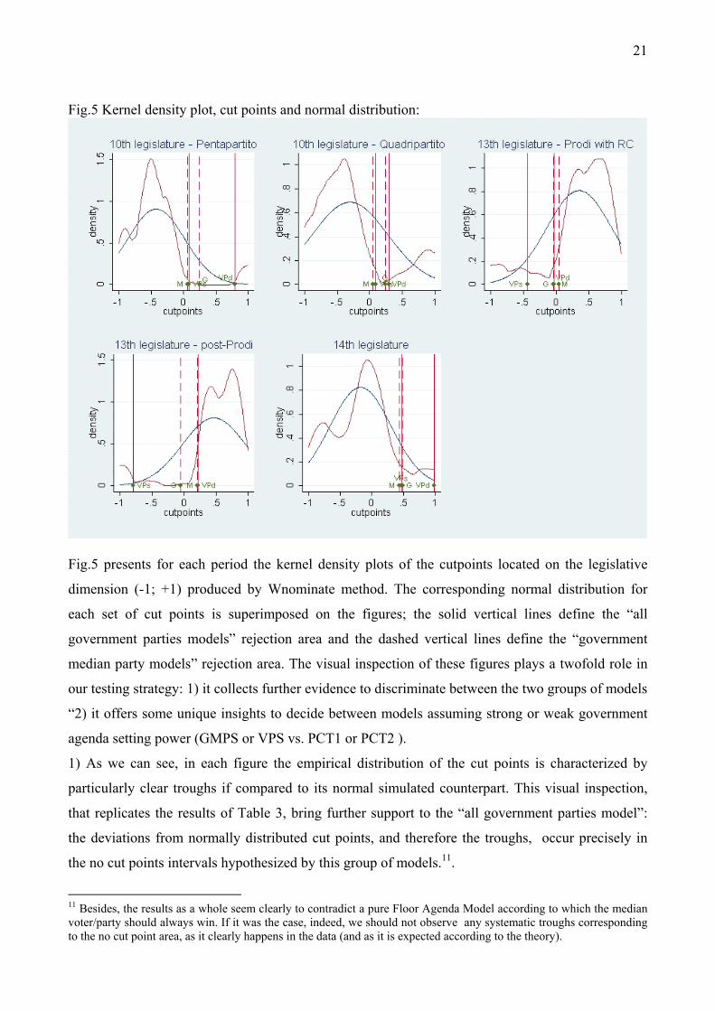
Fig.5 Kernel density plot, cut points and normal distribution:

Fig.5 presents for each period the kernel density plots of the cutpoints located on the legislative

dimension (-1; +1) produced by Wnominate method. The corresponding normal distribution for

each set of cut points is superimposed on the figures; the solid vertical lines define the “all

government parties models” rejection area and the dashed vertical lines define the “government

median party models” rejection area. The visual inspection of these figures plays a twofold role in

our testing strategy: 1) it collects further evidence to discriminate between the two groups of models

“2) it offers some unique insights to decide between models assuming strong or weak government

agenda setting power (GMPS or VPS vs. PCT1 or PCT2 ).

1) As we can see, in each figure the empirical distribution of the cut points is characterized by

particularly clear troughs if compared to its normal simulated counterpart. This visual inspection,

that replicates the results of Table 3, bring further support to the “all government parties model”:

the deviations from normally distributed cut points, and therefore the troughs, occur precisely in

the no cut points intervals hypothesized by this group of models.11.

11 Besides, the results as a whole seem clearly to contradict a pure Floor Agenda Model according to which the median voter/party should always win. If it was the case, indeed, we should not observe any systematic troughs corresponding to the no cut point area, as it clearly happens in the data (and as it is expected according to the theory).

22

2) As we already written (look also the fig.??), according to the VPM model we should expect an

high density of cut points around the position of the two parties defining the gridlock area (i.e., VPs

and VPd), given that for any localizations of the status quo within [2VPs-G, VPs] and [2VPd-G,

VPd] the final cut point position according to the this model should be, respectively, VPs or VPd

(see the first section). In other terms for a more or less extended segment of possible status quos, the

cut points should coincide or being located nearby the position of one of the two extreme

government parties. Viceversa, if PCT2 had to prevail, the distribution of the cut points should not

to show such a concentration around the same points (VPD and VPS) . As we can see from the

figures, there are no peak are around these critical points12. Therefore the model that seems to

represent more correctly the law making in the Italian Chamber of Deputies is the PCT2 model, a

model that does not assume a strong government agenda setting power.

Till now we have focused our analysis on the entire set of roll-calls without differentiating between

bills sponsored by the government and bills promoted by a MP. Even if (see Table 1) the vast

majority of roll-calls involves the first type of bills (9 out of 10), a distinct analysis of the cut points

according to the type of bills could further refine our test. Let’s focus here just on the model more

supported by our empirical data (PCT2 ). In this case, we should expect far less cut points within

the rejection area (in a perfect world, 0) when we deal with government sponsored bills rather than

when we deal with bills sponsored by the MPs. The legislative process of the first category of bills

mirrors quite well what is described in the model. As in our models the first mover is a government

agent and the proposal arrives to the parliamentary floor only if the other government party leaders

(often the ministers) agree. In other terms in the legislative game the formal or informal promoter is

the government as in the reality. The legislative process of a parliamentary bill is less well

represented by the same model as in this case the promoter is located in another institution and the

sequence of the law making process is various and somehow more intricate. The results of Table 4

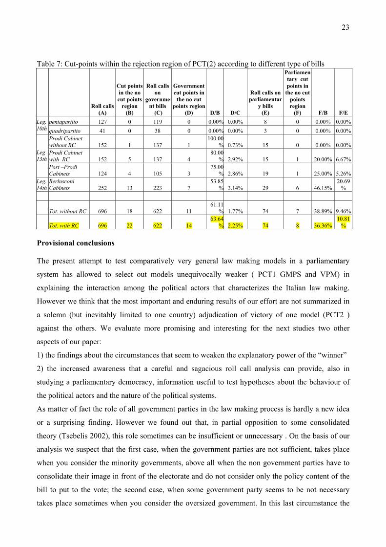
clearly support what we have just emphasized. More than one-third of the overall cut points that fall

within the rejection area of PCT2 is associated to a bill promoted by a MP when the percentage of

parliamentary bills on the bills considered in the roll call analysis is around 10%. Moreover, the

percentage of the bills promoted by a MP whose cut points falls within the rejection area is

remarkable (on average 10%) and much higher than the percentage of the similar bills sponsored by

the government (2.2%).

12 It is possible to test indirectly VPM versus PCT2 also by checking the existence of a relationship between the extension of the segments VPS- 2VPS-G and VPD-2VPD and the density of cut points around respectively VPS and VPD. Indeed if the VPM model fitted well the data we should expect many cut points around the VP actors when this extension increases. The results of this more accurate test confirms what found by the visual inspection.

23

Table 7: Cut-points within the rejection region of PCT(2) according to different type of bills

Roll calls

(A)

Cut points in the no cut points

region (B)

Roll calls on

government bills

(C)

Government cut points in

the no cut points region

(D) D/B D/C

Roll calls on parliamentar

y bills (E)

Parliamentary cut points in

the no cut points region

(F) F/B F/E pentapartito 127 0 119 0 0.00% 0.00% 8 0 0.00% 0.00%Leg.

10th quadripartito 41 0 38 0 0.00% 0.00% 3 0 0.00% 0.00%Prodi Cabinet without RC 152 1 137 1

100.00% 0.73% 15 0 0.00% 0.00%

Prodi Cabinet with RC 152 5 137 4

80.00% 2.92% 15 1 20.00% 6.67%

Leg 13th

Post –Prodi Cabinets 124 4 105 3

75.00% 2.86% 19 1 25.00% 5.26%

Leg.14th

Berlusconi Cabinets 252 13 223 7

53.85% 3.14% 29 6 46.15%

20.69%

Tot. without RC 696 18 622 11 61.11

% 1.77% 74 7 38.89% 9.46%

Tot. with RC 696 22 622 14 63.64

% 2.25% 74 8 36.36%10.81

% Provisional conclusions The present attempt to test comparatively very general law making models in a parliamentary

system has allowed to select out models unequivocally weaker ( PCT1 GMPS and VPM) in

explaining the interaction among the political actors that characterizes the Italian law making.

However we think that the most important and enduring results of our effort are not summarized in

a solemn (but inevitably limited to one country) adjudication of victory of one model (PCT2 )

against the others. We evaluate more promising and interesting for the next studies two other

aspects of our paper:

1) the findings about the circumstances that seem to weaken the explanatory power of the “winner”

2) the increased awareness that a careful and sagacious roll call analysis can provide, also in

studying a parliamentary democracy, information useful to test hypotheses about the behaviour of

the political actors and the nature of the political systems.

As matter of fact the role of all government parties in the law making process is hardly a new idea

or a surprising finding. However we found out that, in partial opposition to some consolidated

theory (Tsebelis 2002), this role sometimes can be insufficient or unnecessary . On the basis of our

analysis we suspect that the first case, when the government parties are not sufficient, takes place

when you consider the minority governments, above all when the non government parties have to

consolidate their image in front of the electorate and do not consider only the policy content of the

bill to put to the vote; the second case, when some government party seems to be not necessary

takes place sometimes when you consider the oversized government. In this last circumstance the

24

weak veto player should be the government party not numerically necessary and most distant from

the floor median voter. We found also that the nature of the promoter (Government versus MP)

matters: the prevailing model to explain the law making in the parliamentary system “fails” much

more often when the bill sponsor is an MP.

The roll call analysis and the linked analysis of cut points promise to help the research on at least

two topics. The location of the cut points could help to establish the consensual or confrontational

nature of a political system according to the voting behaviour in the parliament. The dispersion of

the Mps ideal points around their party median and around the government median can help to

establish, maybe in a more appropriate way, the level of party cohesion and government cohesion.

References Clinton J.D. – S. Jackman – D. River (2004), The Statistical Analysis of Roll Call Data, American Political Science Review, 98(2): 355-70 Clinton J.D. (2007), Lawmaking and Roll Calls, The Journal of Politics, 69(2), 457-69 Gary W. Cox and Mathew D. McCubbins, (2005), Setting the Agenda: Responsible Party Government in the US House of Representatives, Cambridge: Cambridge University Press,. Cox G.W., W.B.Heller and M.D. McCubbins (2008), Agenda Power in the Italian Chamber of Deputies, 1988-2000, Legislative Studies Quarterly, Forthcoming Jun Hae-Won – S. Hix (2006), A Spatial Analysis of Voting in the Korean Assembly, research paper Keith Krehbiel “Pivots” (2006) in In Donald Wittman and Barry Weingast (eds.), Oxford Handbook of Political Economy. New York: Oxford University Press. Krehbiel, Keith. (1998). Pivotal Politics: A Theory of U.S. Lawmaking. Chicago: University of Chicago Press. Krehbiel, K. – A. Meirowitz – J. Woon (2005), Testing Theories of Lawmaking, in Social Choice and Strategic Decisions: Essays in Honor of Jeffrey S. Banks, eds. D-A. Smith and J. Duggan, New York: Springer Laver M. - Schofield N. (1991) Multiparty government, Oxford University Press Laver, M. - Hunt B.(1992). Party and Policy Competition, London: Routledge. Laver M. (2006), Legislatures and Parliaments in Comparative Context, in The Oxford Handbook of Political Economy, eds. B.R. Weingast and D.A.Wittman, Oxford: Oxford University Press, 121:40 Poole K. (2005), Spatial Models of Parliamentary Voting. New York: Cambridge University Press

25

Poole, Keith T. and Howard Rosenthal. (1997). Congress: A Political-Economic History of Roll Call Voting. New York, NY: Oxford University Press. Roberts J.M. (2007), The Statistical Analysis of Roll-Call Data: A Cautionary Tale, Legislative Studies Quarterly, XXXII, 3, 341:60 Rosenthal H. – E. Voeten (2004), Analyzing Roll Calls with Perfect Spatial Voting: France 1946-1958, American Journal of Political Science, Vol.48(3), 620:32 Spirling A. – I. McLean (2007), UK OC OK? Interpreting Optimal Classification Scores for the U.K. House of Commons, Political Analysis, 15: 85-96 Tsebelis G. (2002) Veto Players. How political institutions work. Princeton University Press Voeten E. (2000), Clashes in the Assembly, International Organization, 54(2), 185-215