testing the masters hypothesis in commodity futures markets
TRANSCRIPT

Energy Economics 34 (2012) 256–269
Contents lists available at SciVerse ScienceDirect
Energy Economics
j ourna l homepage: www.e lsev ie r .com/ locate /eneco
Testing the Masters Hypothesis in commodity futures markets
Scott H. Irwin a,1, Dwight R. Sanders b,⁎a University of Illinois at Urbana-Champaign, Carbondale, 344 Mumford Hall, 1301 W. Gregory Drive, Urbana, IL, 61801, United Statesb Southern Illinois University, 226E Agriculture Building, 1205 Lincoln Drive, Carbondale, IL, 62901, United States
⁎ Corresponding author. Tel.: +1 618 453 1711; fax:E-mail addresses: [email protected] (S.H. Irwin), dw
1 Tel.: +1 217 333 6087; fax: +1 217 333 5538.2 See USS/PSI (2009), Irwin, Sanders, and Merrin (2
detailed discussions of the controversy surrounding ththe 2007–2008 commodity price spike.
3 Investors may enter directly into over-the-countedealers to gain the desired exposure to returns from aprices. Some firms also offer investment funds whose reindex. Exchange-traded funds (ETFs) and structureddeveloped that track commodity indexes. In the rema‘commodity index fund’ or ‘index fund’ is used genericmodity investments. See Engelke and Yuen (2008) for fudex investments.
0140-9883/$ – see front matter. Published by Elsevier Bdoi:10.1016/j.eneco.2011.10.008
a b s t r a c t
a r t i c l e i n f oArticle history:Received 13 January 2011Received in revised form 1 July 2011Accepted 7 October 2011Available online 12 October 2011
JEL classification:D84G12G13G14Q13Q41
Keywords:CommodityFutures marketIndex fundsMichael MastersPrice
The ‘Masters Hypothesis’ is the claim that long-only index investmentwas amajor driver of the 2007–2008 spikein commodity futures prices and energy futures prices in particular. Index position data compiled by the CFTC arecarefully compared. In the energymarkets, index position estimates based on agricultural markets are shown tocontain considerable error relative to the CFTC's Index Investment Data (IID). Fama–MacBeth tests using theCFTC's quarterly IID find very little evidence that index positions influence returns or volatility in 19 commodityfutures markets. Granger causality and long-horizon regression tests also show no causal links between dailyreturns or volatility in the crude oil and natural gas futures markets and the positions for two large energyexchange-traded index funds. Overall, the empirical results of this study offer no support for the MastersHypothesis.
Published by Elsevier B.V.
1. Introduction
Commodity futures prices spiked in 2007—2008, led by an in-crease in crude oil futures prices to a new (nominal) all-time highof $145 per barrel. As the spike developed, concerns emerged thatthe increase was being driven by inflows into new commodityindex investments.2 These financial investments are packaged in avariety forms but share a common goal—provide the investor withlong-only exposure to returns from an index of commodity prices.3
For example, the S&P GSCI™ is one of the most widely tracked com-modity indexes and generally considered an industry benchmark. It
+1 618 453 [email protected] (D.R. Sanders).
009), and Pirrong (2010) fore role of index investment in
r (OTC) contracts with swapparticular index of commodityturns are tied to a commoditynotes (ETNs) also have beeninder of this paper, the termally to refer to long-only com-rther details on commodity in-
.V.
is computed as a production-weighted average of the prices from 24commodity futures markets with a relatively heavy weighting towardsenergy markets.
Hedge fundmanager Michael W. Masters is a leading proponent ofthe view that commodity index investment was a major driver of thespike in commodity futures prices. He has testified numerous timesbefore the U.S. Congress and Commodity Futures Trading Commission(CFTC) with variations of the following argument:
“Institutional Investors, with nearly $30 trillion in assets undermanagement, have decided en masse to embrace commoditiesfutures as an investable asset class. In the last five years, theyhave poured hundreds of billions of dollars into the commoditiesfutures markets, a large fraction of which has gone into energyfutures. While individually these Investors are trying to do theright thing for their portfolios (and stakeholders), they are un-aware that collectively they are having a massive impact on thefutures markets that makes the Hunt brothers pale in comparison.In the last 4½, years assets allocated to commodity index replica-tion trading strategies have grown from $13 billion in 2003 to$317 billion in July 2008. At the same time, the prices for the 25commodities that make up these indices have risen by an averageof over 200%. Today's commodities futures markets are excessivelyspeculative, and the speculative position limits designed to protect

257S.H. Irwin, D.R. Sanders / Energy Economics 34 (2012) 256–269
themarkets have been raised, or in some cases, eliminated. Congressmust act to re-establish hard and fast position limits across all mar-kets.” (Masters and White, 2008, p. 1).
In essence, Masters argues that massive buy-side ‘demand’ fromindex funds created a bubble in commodity prices, with the resultthat prices, and crude oil prices in particular, far exceeded fundamen-tal values at the peak. We use the term ‘Masters Hypothesis’ as ashort-hand label for this argument.
As highlighted in the above quote the regulatory response to con-cerns about the impact of index investments in commodity futuresmarkets centers on speculative position limits. Limits on speculativepositions in U.S. agricultural futures markets have been set by theCFTC and its precursors for decades.4 The CFTC proposed to basicallyextend this regulatory regime to four energy futures markets in early2010. The fact that the CFTC received over 8000 responses during thepublic comment period for the proposed rule-making (Acworth andMorrison, 2010), the second highest number of responses in its 36-year history, highlights the economic importance of the policy debatesurrounding commodity index investments. Most recently, the 2010Dodd–Frank Wall Street Reform and Consumer Protection Act grantedthe CFTC broad authority to set aggregate speculative position limitson futures and swap positions in all non-exempt ‘physical commoditymarkets’ in the U.S.
From a theoretical perspective, the impact of index funds in com-modity futures markets hinges on the predictability of their positionchanges. If position changes are perfectly predictable, index fundswill not have an impact in a rational expectations equilibrium be-cause other market participants will anticipate their activity, tradeagainst them, and thereby negate any potential impact (De Longet al., 1990). If index fund position changes are less than perfectlypredictable, a market impact is possible. However, unpredictabilityof index fund activity is a necessary but not sufficient condition fora market impact. For example, assume index fund position changesare unpredictable but related to changing fundamentals (speculationin the traditional sense) then the changes would be positively corre-lated with contemporaneous or subsequent changes in commodityfutures prices, but this would be a reflection of valuable informationon fundamentals rather than a ‘flow’ impact.
One might expect actual index position changes to be highly pre-dictable since most funds track well-known commodity indexes andpublish their mechanical procedures for ‘rolling’ to new contractmonths. However, this ignores the fact that positions also changedue to investment flows into and out of index funds and these maybe quite large. A more plausible scenario is one where index fund posi-tion changes are largely unpredictable and unrelated to market funda-mentals, since portfolio diversification is a main driver of investmentin index funds (Stoll and Whaley, 2010) and this has the effect ofmaking index positions “…insensitive to the supply and demand funda-mentals” (Masters andWhite, 2008, p. 29). Prices could be impacted forseveral reasons under this scenario:
(i) The commodity futures market may not be sufficiently liquid toabsorb the large order flow of index funds. This implies pricesare temporarily pushed away from fundamental value. Sincethe impact is temporary, contemporaneous index fund positionand price changes are positively correlated and current positionchanges and subsequent price changes are negatively correlated.This is the classic problem of illiquidity arising from the asyn-chronous arrival of traders to the marketplace (Grossman andMiller, 1988).
4 A detailed history of position limit regulations in U.S. commodity futuresmarkets can befound at: http://www.cftc.gov/PressRoom/SpeechesTestimony/berkovitzstatement072809.html.
(ii) Index investors are in effect noise traders who make arbitragerisky. This opens the possibility of index investors ‘creatingtheir own space’ if their positions are large enough (De Longet al., 1990). Once again a positive contemporaneous correla-tion is implied between index position changes and pricechanges; however, subsequent price changes may be positivelyor negatively correlated with the current position changedepending on whether prices are pushed above or belowfundamentals.
(iii) Other traders in commodity futures markets have difficultydistinguishing signals from noise. The large order flow ofindex funds on the long side of the market may be seen as areflection of valuable private information about commodityprice prospects, which has the effect of driving the futuresprice higher as other traders subsequently revise their owndemands upward (Grossman, 1986). This increase in theexpected future cash price leads to an increase in inventoriesand also raises current cash prices (Hamilton, 2009). Indexposition changes are positively correlatedwith contemporaneousprice changes, and possibly, subsequent price changes if thereaction of other traders to index order flow is not instantaneous.
However plausible from a logical standpoint, it is nonetheless anempirical question whether these types of impacts are discernablein actual market observations.
Several recent studies test whether there is a statistical link be-tween market positions of index funds and commodity futures pricemovements.5 Gilbert (2009) reports evidence of a significant rela-tionship between index fund trading activity and returns in threecommodity futures markets: crude oil, aluminum, and copper. Heestimates the maximum impact of index funds in these markets tobe a price increase of 15%. In subsequent work, Gilbert (2010) findsevidence of significant relationship between index fund trading andfood price changes. Singleton (2011) estimates a regression modelof crude oil futures prices and finds that index investment flows arean important determinant of price changes along with several otherconditioning variables. His estimates indicate that a 1 million contractincrease in index fund positions in WTI crude oil over the previous13 week period results in a 0.272% increase in nearby crude oil fu-tures prices in the next week. Both Gilbert (2009, 2010) and Singleton(2011) rely on measures of index positions in energy markets im-puted from positions held in agricultural commodities.
Alternatively, Brunetti and Buyuksahin (2009) conduct a batteryof Granger causality tests and do not find a statistical link betweenswap dealers positions (a proxy for commodity index fund positions)and subsequent returns or volatility in the crude oil, natural gas, andcorn futures markets. Stoll and Whaley (2010) also use a variety oftests, including Granger causality tests, and find no evidence thatthe position of commodity index traders impacts prices in agriculturalfutures markets. Sanders and Irwin (2010, 2011a, 2011b) report similarresults for agricultural and energy futures markets. Buyuksahin andHarris (2011) do not find a statistical link between swap dealerspositions and changes in crude oil futures prices. Buyuksahin andRobe (2011) show that index fund activity (again, as measured byswap dealer positions) is not associated with the increasing correlationbetween commodity and stock returns.
Irwin and Sanders (2011) survey this literature and conclude thatthe weight of the available empirical evidence tilts against theMasters Hypothesis. However, proponents of the Masters Hypothesissharply criticize the data and methods used in the studies that fail to
5 Other studies investigate the impact of speculation in the recent commodity pricespike without directly testing for statistical linkages between index fund positions andprice movements (e.g., Einloth, 2009; Kilian and Murphy, 2010; Phillips and Yu, 2010;and Tang and Xiong, 2010). Conclusions are mixed with regard to the impact of spec-ulation or whether a price bubble occurred.

258 S.H. Irwin, D.R. Sanders / Energy Economics 34 (2012) 256–269
detect a market impact of index fund investment.6 The first criticismis due to reliance on the CFTC's Commitments of Traders (COT) data-base of the positions held by reporting traders. In this database thefutures positions of swap dealers represent the net of long commod-ity index positions with other long and short over-the-counter (OTC)positions and this may mask the true level of index investment incommodities markets. That is, to the degree that long and short OTCpositions are internally netted by swap dealers in a particular com-modity market, the futures positions reported to the CFTC by swapdealers may not accurately reflect the total effective ‘demand’ ofindex investors. The second criticism is that the impact of indexinvestment is estimated for daily or weekly time horizons; shorterthan the time horizon implicit in the Masters Hypothesis. While thehorizon is not stated explicitly, the basic idea is that a ‘wave’ ofindex investment pressures commodity futures prices over muchlonger time intervals such as a month or a quarter. This is similar tothe argument of Summers (1986) and others regarding tests for aslowly accumulating ‘fads’ component in stock returns. The thirdcriticism is that nearly all of the studies employ time-series Grangercausality tests, which may lack the statistical power necessary toreject the null hypothesis of non-causality because the dependentvariable—the change in commodity futures prices—is extremely volatile.
The present study addresses criticisms of previous work by usingnewdata that bettermatches the basic tenets of theMasters Hypothesisand applyingmore powerful statistical tests. The CFTC's quarterly IndexInvestment Data (IID) report provides the best measure of actual com-modity index investment and our study is the first to use these data inempirical tests. The IID data are not only a better measure of indexinvestment—because positions are measured before internal nettingby swap dealers—it also covers the complete spectrum of agricultural,energy, metal, and soft commodity futures markets. A cross-sectionalFama–MacBeth regression test is applied to the IID positions at aquarterly horizon. Ibragimov and Muller (2010a,b) show that theFama–MacBeth test has good power properties for the sample sizesconsidered here. Quarterly horizons should capture slowly accumulat-ing price pressure if it is present in the data. Consistent with theory,both lagged and contemporaneous effects are considered as well.
We supplement the cross-sectional tests using a large sample ofdaily positions held by the U.S. Oil and Natural Gas Funds, two ofthe largest exchange-traded index funds (ETFs), in the crude oil andnatural gas futures markets, respectively. In order to address powerconcerns, both Granger causality and long-horizon regression tests(Valkanov, 2003) are applied to the daily time-series of ETF positions.
Fama–MacBeth tests using the quarterly IID positions reveal verylittle evidence that index positions influence returns or volatility in19 commodity futures markets. The cross-sectional IID results arerobust to whether lagged or contemporaneous effects are consideredand the addition of the nearby-deferred futures spread as a condition-ing variable. Granger-causality tests show no causal links betweendaily returns or volatility in crude oil and natural gas futures marketsand the positions of the two large ETFs. Long-horizon regression testslikewise fail to reject the null hypothesis of no market impact for theETFs. Overall, the empirical results of this study fail to support theMasters Hypothesis.
2. Measures of commodity index fund investment
A key issue in testing the Masters Hypothesis is themeasurement ofindex fund investment in commodity futures markets. Private vendorshave collected data for over a decade; however, only the aggregatedollar investment is available for all markets combined. As noted inthe introduction, the CFTC has developed several data series on
6 For an example, see the letter “Swaps, Spots, and Bubbles” by Sir Richard Branson,Michael Masters, and David Frenk published in the July 29, 2010 issue of the Economistmagazine (http://www.economist.com/node/16690679).
commodity index fund investment and/or positions by individual fu-tures market. Since these data are used in nearly all previous studieson the market impact of commodity index investment, as well as thepresent study, it is important to understand how the data are collectedand categorized as well as any limitations.
2.1. Commitments of Traders (COT) reports
The core of the CFTC's market surveillance program is the LargeTrader Reporting System (LTRS) established under the CommodityExchange Act (CEA). The CEA authorizes the CFTC to collect marketdata and position information from market participants who haveposition levels above the reporting level for a specific futures market(CFTC, 2010c). The CFTC is prohibited from disclosing the positionsheld by individuals, but they have long categorized traders withinthe system as those traders who are largely hedgers (commercials)and those that are largely speculating (non-commercials). The classi-fication of traders is heavily based on the information provided bytraders in the CFTC's Form 40, where traders must describe the natureof their futures transactions (including the associated physical marketactivities, if any).
The CFTC releases the combined futures and delta-adjusted optionpositions aggregated by trader category each Friday in the Futures-and-Options-Combined Commitments of Traders (COT) report. Openinterest reflects Tuesday's closing positions for a given market and isaggregated across all contract expiration months. Non-commercialopen interest is divided into long, short, and spreading; whereas,commercial and non-reporting open interest is simply divided intolong or short. The following relation explains how the market's totalopen interest (TOI) is disaggregated:
NCLþ NCSþ 2 NCSPð Þ½ � þ CLþ CS½ �|fflfflfflfflfflfflfflfflfflfflfflfflfflfflfflfflfflfflfflfflfflfflfflfflfflfflfflfflfflfflfflfflfflffl{zfflfflfflfflfflfflfflfflfflfflfflfflfflfflfflfflfflfflfflfflfflfflfflfflfflfflfflfflfflfflfflfflfflffl}Reporting
þ NRLþ NRS½ �|fflfflfflfflfflfflfflfflffl{zfflfflfflfflfflfflfflfflffl}Non−Reporting
¼ 2 TOIð Þ; ð1Þ
where NCL, NCS, and NCSP are non-commercial long, short, and spread-ing positions, respectively. CL (CS) represents commercial long (short)positions, and NRL (NRS) are long (short) positions held by non-reporting traders. Reporting and non-reporting positions must sum tothe market's total open interest (TOI), and the number of longs mustequal the number of short positions.
There have been ongoing complaints that the legacy COT trader desig-nationsmay be inaccurate (e.g., Ederington and Lee, 2002). As one exam-ple, speculators may have an incentive to self-classify their activity ascommercial hedging to circumvent speculative position limits in somemarkets. But, the CFTC implements a fairly rigorous process—includingstatements of cash positions in the underlying commodity—to ensurethat commercial traders have an underlying risk associatedwith futurespositions. However, in recent years industry participants began to sus-pect that these data were contaminated because the underlying riskformany reporting commercials was not a position in the physical com-modity (CFTC, 2006a,b). Rather, the reporting commercials were banksand other swap dealers hedging risk associated with over-the-counter(OTC) derivative positions.
In response to these concerns the CFTC added two variations to thelegacy COT reports. Thefirst is theDisaggregated Commitments of Traders(DCOT) report which, as the title suggests, simply further disaggregatesthe legacy COT commercial and non-commercial trader categories. Thesecond report, Supplemental Commitments of Traders (SCOT) adds a newcategory specifically to capture commodity index traders.
2.2. Disaggregated Commitments of Traders (DCOT) report
The CFTC began publishing the Disaggregated Commitments ofTraders (DCOT) report in September 2009 and ultimately provid-ed historical data back to June 2006 (CFTC, 2009). The DCOT dataare available for most commodity futures markets. Constructed in

259S.H. Irwin, D.R. Sanders / Energy Economics 34 (2012) 256–269
a manner analogous to the legacy reports, DCOT reports breakdown combined futures and options positions as follows:
SDLþ SDSþ 2 SDSPð Þ½ � þ MMLþMMSþ 2 MMSPð Þ½ � þ PMLþ PMS½ � þ ORLþ ORSþ 2 ORSPð Þ½ �|fflfflfflfflfflfflfflfflfflfflfflfflfflfflfflfflfflfflfflfflfflfflfflfflfflfflfflfflfflfflfflfflfflfflfflfflfflfflfflfflfflfflfflfflfflfflfflfflfflfflfflfflfflfflfflfflfflfflfflfflfflfflfflfflfflfflfflfflfflfflfflfflfflfflfflfflfflfflfflfflfflfflfflfflfflfflfflfflfflfflfflfflfflfflffl{zfflfflfflfflfflfflfflfflfflfflfflfflfflfflfflfflfflfflfflfflfflfflfflfflfflfflfflfflfflfflfflfflfflfflfflfflfflfflfflfflfflfflfflfflfflfflfflfflfflfflfflfflfflfflfflfflfflfflfflfflfflfflfflfflfflfflfflfflfflfflfflfflfflfflfflfflfflfflfflfflfflfflfflfflfflfflfflfflfflfflfflfflfflfflffl}Reporting
þ NRLþ NRS½ �|fflfflfflfflfflfflfflfflffl{zfflfflfflfflfflfflfflfflffl}Non−Reporting
¼ 2 TOIð Þ; ð2Þ
where reporting non-commercial traders are disaggregated intomanaged money (MM) and other reportables (OR). Commercialtraders from the legacy COT reports are segregated into proces-sors and merchants (PM) as well as swap dealers (SD). Positionsare divided into long (L), short (S), and spreading (SP) as indicat-ed by the corresponding suffixes. For example, the SDL, SDS, andSDSP are the swap dealers' long, short, and spreading positions,respectively.
Taken from the legacy commercial category, swap dealers (SD) arethose traders who deal primarily in swaps and hedge those transactionsin the futures market. There is considerable uncertainty whether swapdealer positions represent an underlying speculative or hedging posi-tion. A large portion of swap dealers' trading represents commodityindex investors and swap dealer positions are often used as a proxyfor their activity (e.g., Brunetti and Buyuksahin, 2009; Buyuksahin andHarris, 2011; Sanders and Irwin, 2011b). Processors and merchants(PM) include traditional commercial users—processors and producersof the commodity who are actively engaged in the physical marketsand are using the futures to hedge associated price risks.
Disaggregated from the legacy non-commercial category, managedmoney (MM) represents positions held by commodity trading advisors,commodity pool operators and hedge funds that manage and conductfutures trading on behalf of clients. The traders included in themanagedmoney category would largely represent the more traditional class ofspeculative traders. Other reportable (OR) are non-commercial traderswho are large enough to report but do not fit into one of the othercategories. These might include large individual speculative traders ormarket-makers as well as firms managing their own assets. For swapdealers, managed money and other reportables, offsetting long andshort positions in the same market but with different contract monthsare reported as spreading positions. Index investment positions in theDCOT report can be a part of the swap dealers, managed money, andother reportable categories.
Legacy COT Report Disaggregated COT
Commercials
Non-Commercials
Non-Reporting
Processors & Mercha
Managed Money
Non-Reporting
Swap Dealers
Other Reportables
Fig. 1. Relationship between legacy, disaggregated, an
2.3. Supplemental Commitments of Traders (SCOT) report
Starting in 2007, the CFTC began releasing the Supplemental Commit-ments of Traders (SCOT) reports (sometimes referred to as the commod-ity index traders or CIT report), which specifically breaks out thepositions of index traders for 12 agricultural markets. Index traders areidentified by reviewing the CFTC Form 40 and through confidential in-terviews with traders known to be index traders or who exhibit tradingpatterns consistent with indexing (CFTC, 2010a). It is important to notethat the CFTC does not distinguish index and non-index positions in thisprocess. So, if a trader is identified as an index trader, then all of their po-sitions are counted as index positions. In addition, the index trader posi-tions reflect both institutional investment funds that would havepreviously been classified as non-commercials in the legacy COT reportsas well as swap dealers who would have previously been classified ascommercials hedging OTC transactions. Sanders, Irwin and Merrin(2010) show that approximately 85% of index trader positions in the12 SCOT markets are in fact drawn from the long commercial categorywith the other 15% from the long non-commercial category. This impliesthat the bulk of index positions in the 12 SCOT markets are initiallyestablished in the OTCmarket and the underlying position is then trans-mitted to the futures market by swap dealers hedging OTC exposure.
The supplemental data are released in conjunction with the legacyCOT report showing combined futures and options positions. The indextrader positions are simply removed from their prior categories and pre-sented as a new category of reporting traders. The supplemental data in-clude the long and short positions held by commercials (less indextraders), non-commercials (less index traders), index traders, and non-reporting traders aggregated across all contracts for a particular market:
NCL−CITLð Þ þ NCS−CITSð Þ þ 2 NCSPð Þ½ � þ CL−CITLð Þ þ CS−CITSð Þ½ � þ CITLþ CITS½ �|fflfflfflfflfflfflfflfflfflfflfflfflfflfflfflfflfflfflfflfflfflfflfflfflfflfflfflfflfflfflfflfflfflfflfflfflfflfflfflfflfflfflfflfflfflfflfflfflfflfflfflfflfflfflfflfflfflfflfflfflfflfflfflfflfflfflfflfflfflfflfflfflfflfflfflfflfflfflfflfflfflfflfflfflfflffl{zfflfflfflfflfflfflfflfflfflfflfflfflfflfflfflfflfflfflfflfflfflfflfflfflfflfflfflfflfflfflfflfflfflfflfflfflfflfflfflfflfflfflfflfflfflfflfflfflfflfflfflfflfflfflfflfflfflfflfflfflfflfflfflfflfflfflfflfflfflfflfflfflfflfflfflfflfflfflfflfflfflfflfflfflfflffl}Reporting
þ NRLþ NRS½ �|fflfflfflfflfflfflfflfflffl{zfflfflfflfflfflfflfflfflffl}Non−Reporting
¼ 2 TOIð Þ: ð3Þ
The above relation is analogous to that for the traditional COTreport shown in Eq. (1), except commercial and noncommercial posi-tions are adjusted for the commodity index trader long (CITL) andindex trader short (CITS) positions.
There is a relatively straightforward disaggregation of the legacyCOT categories into the DCOT categories and then back into the SCOTclassifications as shown in Fig. 1. In this illustration, the source of
Report Supplemental COT Report
nts
Commercials (less index traders)
Non-Commercials (less index traders)
Index Traders
Non-Reporting
d supplemental commitments of traders reports.

Table 1Notional value of net long index fund positions based on Index Investment Data (IID)and comparisons to popular commodity indices, March 31, 2010.
Commodityfutures market
IID notional value(billion $)
IIDportfolioweight
S&P-GSCIportfolioweight
DJ-UBSportfolioweight
RJ-CRBporfolioweight
Corn 6.9 4.3% 3.1% 6.6% 6.0%Soybeans 8.0 5.0% 2.2% 7.9% 6.0%Soybean oil 2.2 1.4% 0.0% 3.0% 0.0%Wheat, CBOT 5.5 3.4% 2.8% 4.4% 1.0%Wheat, KCBT 0.7 0.4% 0.6% 0.0% 0.0%Cotton 3.0 1.9% 1.2% 2.4% 5.0%Live cattle 5.1 3.2% 2.7% 4.0% 6.0%Feeder cattle 0.5 0.3% 0.5% 0.0% 0.0%Lean hogs 2.9 1.8% 1.8% 2.8% 1.0%Coffee 2.7 1.7% 0.7% 2.5% 5.0%Sugar 3.8 2.4% 1.5% 1.6% 5.0%Cocoa 0.7 0.4% 0.4% 0.0% 5.0%WTI crude oil 36.4 22.6% 36.4% 15.7% 23.0%RBOB unleadedgas
7.8 4.8% 4.7% 4.1% 5.0%
Heating oil 6.7 4.2% 4.7% 3.9% 5.0%Natural gas 12.5 7.8% 4.0% 8.4% 6.0%Gold 10.3 6.4% 3.1% 9.8% 6.0%Silver 3.1 1.9% 0.4% 3.4% 1.0%Copper 5.5 3.4% 3.6% 7.7% 6.0%Other U.S.markets
1.4 0.9% 0.0% 0.0% 1.0%
U.S. marketstotal
125.8 78.0% 74.2% 88.0% 93.0%
Non-U.S. marketstotal
35.4 22.0% 25.8% 12.0% 7.0%
All marketstotal
161.2 100.0% 100.0% 100.0% 100.0%
SectorGrains 23.3 14.5% 8.7% 21.8% 13.0%Livestock 10.2 6.3% 3.8% 6.5% 20.0%Softs 8.5 5.3% 5.0% 6.8% 7.0%Metals 18.9 11.7% 7.1% 20.9% 13.0%Energy 63.4 39.4% 49.7% 32.0% 39.0%Other U.S.markets
1.4 0.9% 0.0% 0.0% 1.0%
Non-U.S.markets
35.4 22.0% 25.8% 12.0% 7.0%
Note: In this and subsequent tables, CBOT denotes Chicago Board of Trade and KCBOTdenotes Kansas City Board of Trade.
260 S.H. Irwin, D.R. Sanders / Energy Economics 34 (2012) 256–269
errors in compiling index trader positions from the DCOT data be-comes clear. First, and most obvious, the use of the swap dealer posi-tions in the DCOT as a proxy for index trader positions will clearlyexclude those index positions found in the managed money and theother reportables categories. Second, and less obvious, to the degreethat positions are netted within firms—especially among swapdealers—reportable futures positions will understate true levels ofindex investment.
One can infer from comparisons found in the CFTC's September2008 report on swap dealer positions (CFTC, 2008) that DCOT swapdealer positions in agricultural futures markets correspond reason-ably well to index trader positions. Since swap dealers operating inagricultural markets conduct a limited amount of non-index long orshort swap transactions there is limited error in attributing the netlong futures position of swap dealers in these markets to indexfunds. In contrast, swap dealers in energy futures markets conduct asubstantial amount of non-index swap transactions on both the longand short side of the market, which creates uncertainty about howwell the net long position of swap dealers in energy markets repre-sent index fund positions. For example, the CFTC estimates that only41% of long swap dealer positions in crude oil futures markets onthree dates in 2007 and 2008 were linked to long-only index fundpositions (CFTC, 2008).
In sum, while the netting effect seems to have a relatively modestimpact on the measurement of index investing in agricultural futuresmarkets, it likely creates considerable measurement error for theenergy and metals futures markets. Realizing this, the CFTC utilizedtheir regulatory power to first issue a ‘special call’ in June 2008 to as-sess the total investment activities (on- and off-exchange) of com-modity index funds. The index investment data collected throughthe CFTC's special call provides the most accurate measure of totalcommodity index investment available to date.
2.4. Index Investment Data (IID) report
The on-going ‘special call’ of all swap dealers and index funds knownto be significant users of U.S. futuresmarkets has allowed the CFTC to col-lect the total notional value of the firms' commodity index business andthe equivalent number of futures contracts (CFTC, 2010b). The originalcall in September 2008 gathered data from 43 entities engaging inindex activities in commodity markets. These entities included indexfunds, swap dealers, pension funds, hedge funds, mutual funds, exchangetraded funds (ETFs), and exchange traded notes (ETNs). Since the call in-cluded the financial institutions known to be the largest swap dealers intheworld and all entities granted exemptions fromFederal position limitsor "no action" letters, the coverage of the special call is the most compre-hensive to date in terms of commodity index activity (CFTC, 2008).
Firms subject to the special call report the total notional value ofcommodity index positions, whether the positions are for a firm'sown account or on behalf of a client. Notional value is also reportedseparately for U.S. and non-U.S. markets. Crucially, each firm's entire"book of business" in futures and OTC markets that is related to com-modity index investments is reported, not just the netted amountthat may be managed ultimately in the futures markets. The datareported as part of the special call is cross-checked by comparing itto the positions in the CFTC's larger trader reporting system and byengaging the firms in extensive discussions.
As pointed out by the CFTC (2010b), because the special call correctsfor netting, the positions reported in the Index Investment Data (IID) re-port are is more precise than the SCOT and DCOT in representing indexinvestment. Moreover, because the netting effect that plagues the COTdata is corrected the IID data are more comprehensive in terms of mar-kets covered. The IID is available for the 12 agricultural markets in theSCOT report plus 7 major energy and metals markets. The IID reportdoes have some limitations. First, some small entities or entities un-known to the CFTCmay be omitted from the special call. Second, trading
records are not independently examined by the CFTC. Third, “index”activity is not specifically defined so there could be some inconsistencyin the reported data across firms. Despite these limitations, the com-prehensive nature of the data set makes the IID the best candidate forevaluating potential market impacts from commodity index invest-ments. In thewords of the CFTC, “The index investment data representsthe Commission’s best effort to provide a one-day snapshot of the posi-tions of swap dealers and index funds” (CFTC, 2010b, p. 4).
3. Data and descriptive statistics
3.1. Comparison of IID, DCOT, and SCOT Data
The IID is collected at the end of each quarter from December 31,2007 through March 31, 2011 (14 quarter-end observations). The mar-kets covered by the IID are listed in Table 1 along with the notionalvalues as of March 31, 2010. Table 1 also includes the percentageallocated across markets, and comparable weightings for three popularcommodity indices: S&P-Goldman Sachs Commodity Index™ (SP-GSCI), Dow Jones-UBS Commodity Index™ (DJ-UBS), and the Reuters/Jefferies Commodity Research Bureau Index™ (RJ-CRB). A total of$161.2 billion was invested in commodity index investments as ofMarch 31, 2010. The IID show that 78% of index investments are inU.S. futures markets with the other 22% in non-U.S. markets. Notsurprisingly, the energy markets—crude oil in particular—have the
60
80
100
120
140
160
180
200
220
Dec
-07
Mar
-08
Jun
-08
Sep
-08
Dec
-08
Mar
-09
Jun
-09
Sep
- 09
Dec
-09
Mar
-10
Jun
-10
Sep
-10
Dec
- 10
Mar
- 1
1
Inve
stm
ent (
bil.$
)
Quarter Ending
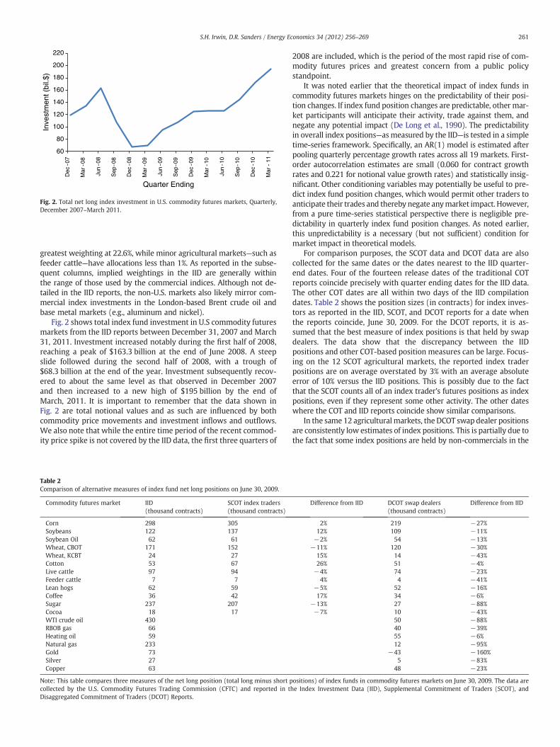
Fig. 2. Total net long index investment in U.S. commodity futures markets, Quarterly,December 2007–March 2011.
261S.H. Irwin, D.R. Sanders / Energy Economics 34 (2012) 256–269
greatest weighting at 22.6%, while minor agricultural markets—such asfeeder cattle—have allocations less than 1%. As reported in the subse-quent columns, implied weightings in the IID are generally withinthe range of those used by the commercial indices. Although not de-tailed in the IID reports, the non-U.S. markets also likely mirror com-mercial index investments in the London-based Brent crude oil andbase metal markets (e.g., aluminum and nickel).
Fig. 2 shows total index fund investment in U.S commodity futuresmarkets from the IID reports between December 31, 2007 and March31, 2011. Investment increased notably during the first half of 2008,reaching a peak of $163.3 billion at the end of June 2008. A steepslide followed during the second half of 2008, with a trough of$68.3 billion at the end of the year. Investment subsequently recov-ered to about the same level as that observed in December 2007and then increased to a new high of $195 billion by the end ofMarch, 2011. It is important to remember that the data shown inFig. 2 are total notional values and as such are influenced by bothcommodity price movements and investment inflows and outflows.We also note that while the entire time period of the recent commod-ity price spike is not covered by the IID data, the first three quarters of
Table 2Comparison of alternative measures of index fund net long positions on June 30, 2009.
Commodity futures market IID(thousand contracts)
SCOT index traders(thousand contracts)
Corn 298 305Soybeans 122 137Soybean Oil 62 61Wheat, CBOT 171 152Wheat, KCBT 24 27Cotton 53 67Live cattle 97 94Feeder cattle 7 7Lean hogs 62 59Coffee 36 42Sugar 237 207Cocoa 18 17WTI crude oil 430RBOB gas 66Heating oil 59Natural gas 233Gold 73Silver 27Copper 63
Note: This table compares three measures of the net long position (total long minus short pcollected by the U.S. Commodity Futures Trading Commission (CFTC) and reported in tDisaggregated Commitment of Traders (DCOT) Reports.
2008 are included, which is the period of the most rapid rise of com-modity futures prices and greatest concern from a public policystandpoint.
It was noted earlier that the theoretical impact of index funds incommodity futures markets hinges on the predictability of their posi-tion changes. If index fund position changes are predictable, other mar-ket participants will anticipate their activity, trade against them, andnegate any potential impact (De Long et al., 1990). The predictabilityin overall index positions—asmeasured by the IID—is tested in a simpletime-series framework. Specifically, an AR(1) model is estimated afterpooling quarterly percentage growth rates across all 19 markets. First-order autocorrelation estimates are small (0.060 for contract growthrates and 0.221 for notional value growth rates) and statistically insig-nificant. Other conditioning variables may potentially be useful to pre-dict index fund position changes, which would permit other traders toanticipate their trades and thereby negate anymarket impact. However,from a pure time-series statistical perspective there is negligible pre-dictability in quarterly index fund position changes. As noted earlier,this unpredictability is a necessary (but not sufficient) condition formarket impact in theoretical models.
For comparison purposes, the SCOT data and DCOT data are alsocollected for the same dates or the dates nearest to the IID quarter-end dates. Four of the fourteen release dates of the traditional COTreports coincide precisely with quarter ending dates for the IID data.The other COT dates are all within two days of the IID compilationdates. Table 2 shows the position sizes (in contracts) for index inves-tors as reported in the IID, SCOT, and DCOT reports for a date whenthe reports coincide, June 30, 2009. For the DCOT reports, it is as-sumed that the best measure of index positions is that held by swapdealers. The data show that the discrepancy between the IIDpositions and other COT-based position measures can be large. Focus-ing on the 12 SCOT agricultural markets, the reported index traderpositions are on average overstated by 3% with an average absoluteerror of 10% versus the IID positions. This is possibly due to the factthat the SCOT counts all of an index trader's futures positions as indexpositions, even if they represent some other activity. The other dateswhere the COT and IID reports coincide show similar comparisons.
In the same 12 agriculturalmarkets, the DCOT swap dealer positionsare consistently low estimates of index positions. This is partially due tothe fact that some index positions are held by non-commercials in the
Difference from IID DCOT swap dealers(thousand contracts)
Difference from IID
2% 219 −27%12% 109 −11%−2% 54 −13%
−11% 120 −30%15% 14 −43%26% 51 −4%−4% 74 −23%
4% 4 −41%−5% 52 −16%17% 34 −6%
−13% 27 −88%−7% 10 −43%
50 −88%40 −39%55 −6%12 −95%
−43 −160%5 −83%
48 −23%
ositions) of index funds in commodity futures markets on June 30, 2009. The data arehe Index Investment Data (IID), Supplemental Commitment of Traders (SCOT), and

Table 4Cross-market correlations of growth rates in index investment net long positions.
Non-SCOT market
WTI RBOB Heating NaturalSCOT market Crude oil Gasoline Oil Gas Gold Silver Copper
Corn −0.40 0.19 0.60 0.63 0.81 0.77 0.42Soybeans −0.36 0.27 0.82 0.52 0.69 0.78 0.42Soybean oil −0.37 0.21 0.88 0.61 0.66 0.59 0.23Wheat, CBOT −0.41 0.30 0.81 0.57 0.77 0.63 0.29Wheat, KCBT −0.31 0.02 0.54 0.23 0.09 0.20 0.04Cotton −0.23 0.23 0.44 0.35 0.54 0.69 0.33Live cattle −0.50 0.19 0.43 0.40 0.87 0.51 0.19Feeder cattle −0.10 0.43 0.08 0.19 0.17 0.21 0.34Lean hogs −0.52 0.23 0.29 0.34 0.76 0.62 0.32Coffee −0.38 0.31 0.19 0.22 0.48 0.77 0.43Sugar −0.07 0.38 0.13 0.33 0.48 0.32 0.59Cocoa −0.37 0.08 0.28 0.46 0.42 0.21 0.18Average −0.34 0.24 0.46 0.41 0.56 0.53 0.31
Note: Simple Pearson correlation coefficients calculated between the log-relativegrowth rates in net trader positions reported in the Index Investment Data (IID) Re-ports. SCOT denotes the Supplemental Commitments of Traders report. The data arebased on end-of-quarter positions between March 31, 2008 and March 31, 2011.
Table 3Correlation between index investment net long positions and alternative measures ofindex positions.
Commodity futuresmarket
IID and SCOT indextraders
IID and DCOT swapdealers
Corn 0.86 0.80Soybeans 0.81 0.88Soybean oil 0.76 0.66Wheat, CBOT 0.76 0.67Wheat, KCBT 0.45 0.47Cotton 0.83 0.72Live cattle 0.95 0.91Feeder cattle 0.73 0.57Lean hogs 0.95 0.93Coffee 0.82 0.71Sugar 0.93 0.59Cocoa 0.85 0.55WTI crude oil 0.13RBOB unleaded gas 0.42Heating oil 0.09Natural gas 0.33Gold −0.36Silver 0.10Copper 0.59
Note: Simple Pearson correlation coefficients are calculated between the changes in nettrader positions reported in the Index Investment Data (IID), SupplementalCommitment of Traders (SCOT), and Disaggregated Commitment of Traders (DCOT)Reports. The data are based on end-of-quarter positions between March 31, 2008 andMarch 31, 2011.
262 S.H. Irwin, D.R. Sanders / Energy Economics 34 (2012) 256–269
managed money and other reportables categories. It is also due to thenetting of positions that occurs within a swap dealer's book. Althoughthe netting effect is expected to be relatively small in the agriculturalmarkets, the average absolute error is still 29% for the 12 agriculturalmarkets. The largest errors are concentrated in sugar and cocoa wherethere is a greater tendency for offsetting non-index OTC transactions.
In the seven non-SCOT energy and metal markets shown inTable 2, the average absolute difference between swap dealer posi-tions and the IID increases markedly to 71%. Indeed, on this date theswap dealer position in the gold market is short, opposite of theIID's long position. Likewise, on other report dates net short swapdealer positions are recorded for silver, sugar, natural gas and crudeoil, whereas the IID only shows net long positions for these markets.This is clear evidence of the netting effect impacting reported DCOTswap dealer positions, where the internal crossing of positions effec-tively masks the total underlying level of index investment.
The differences between the index trader and swap dealer positionsand the IIDmay be irrelevant if themeasures are highly correlated. Cor-relation coefficients (Pearson) of changes in net positions are presentedin Table 3. Consider first the correlation between SCOT positions and IIDpositions. Statistically significant correlations are observed in 11 of the12 SCOTmarkets (10% level for a two-tailed t-test) with an average cor-relation coefficient at 0.81. For the same 12markets, DCOT swap dealerpositions are significantly correlated with IID positions in only 8 mar-kets. The correlation between IID net positions and swap dealer posi-tions breaks down even more in the energy and metals markets,where one of the correlations is negative (gold) and none are statistical-ly different from zero at the 10% level.
It is clear that the single best measure of total commodity indexpositions is that available in the IID report. TheDCOT report's swap dealernet positions are relatively poor proxies for total index positions as theyoften shownegative net long positions that are not statistically correlatedwith IIDpositions in the energy andmetalsmarkets. The SCOT report pro-vides useful measures of index positions in agricultural futures markets.
3.2. Comparison of mapping algorithm to IID
Masters (2008) and others impute index positions for individualcommodity futures markets (e.g., energy and metals) that are not
included in the SCOT report. This is accomplished by taking a SCOTmarket that is unique to a particular index and using the notionalvalue of index trader positions in that market (as reported in theSCOT) to estimate total investment in a particular index. Then, anynon-SCOT market is simply assigned the notional value according toits weight in the index.
As an example, consider the calculation using SCOT data fromDecember 31, 2007 and following the procedure presented in theappendix of Masters (2008). Soybean oil futures had a reported indexposition of 77,752 contracts with a notional value of $2279 million. Soy-bean oil is not included in the S&P-GSCI but is a component of the DJ-UBS commodity index, where it has a weight of 2.85%. Scaling this posi-tion up accordingly (2279/0.0285) yields a total notional investment of$79,965 million in the DJ-UBS index. WTI crude oil receives a weight of12.72% in the index; therefore, the notional value of the crude oil invest-ment stemming fromDJ-UBS investments is $10,172 million or 106,000contracts at $95.98 per barrel. For the S&P-GSCI an analogous process isfollowed using feeder cattle and Kansas City Board of Trade (KCBT)wheat futures, both of which are unique to the S&P-GSCI. The result isa range of possible WTI holdings from 286,000 (imputed via feedercattle) to 468,000 (imputed via KCBT wheat) contracts. Next, the WTIcrude oil contracts attributed to S&P-GSCI and DJ-UBS investments aresummed together to get a total index position inWTI crude oil contractsranging from 392,000 to 574,000 contracts with an average of 483,000.
This mapping algorithm rests on a number of key considerationsthat may not be an accurate reflection of reality (see appendix 2 inBuyuksahin and Robe (2011)). First, it assumes that total investmentis allocated to individual markets according to one of the widely-tracked commodity price indexes. Second, it assumes that fund man-agers strictly adhere to this weighting even in relatively minor mar-kets such as feeder cattle. Third, as shown above, it can generate awide range of estimates depending on the market on which the esti-mates are based. Finally, as pointed out by Singleton (2011), the mea-surement error using this mapping procedure will be amplified by theprocess of scaling minor market positions (such as soybean oil) up tomajor market positions (such as crude oil). For instance, in the exam-ple above, feeder cattle had a weight of 0.47% in the S&P-GSCI whichcreated a scaling factor of 213 for imputing total investment. So, anyerror in the SCOT feeder cattle position for index traders is increasedmany times over in the Masters (2008) scaling procedure.
Indeed, the data generated suggest that the level of error in thesemapping procedures is likely to be quite large. In the example presentedin Masters (2008) errors are of a relatively large magnitude even forSCOT markets. For example, the mapping algorithm under-estimates

300
400
500
600
700
800
900
Dec
-07
Mar
-08
Jun
- 08
Sep
-08
Dec
-08
Mar
-09
Jun
- 09
Sep
-09
Dec
- 09
Mar
-10
Jun
- 10
Sep
-10
Dec
-10
Mar
-11
Con
trac
ts (
1,00
0's)
Quarter Ending
Index Investment Data Masters
Fig. 3. Comparison of quarterly WTI crude oil net long index positions based on IndexInvestment Data (IID) and Masters Algorithm Estimates, December 2007–March 2011.
-80
-60
-40
-20
0
20
40
60
80
De
c-0
7
Mar
-08
Jun-
08
Se
p-0
8
De
c-0
8
Mar
-09
Jun-
09
Se
p-0
9
De
c-0
9
Mar
-10
Jun-
10
Se
p-1
0
De
c-1
0
Mar
-11
Gro
wth
Rat
e (
%)
Quarter Ending
Fig. 4. Growth rate of quarterly Index Investment Data (IID) Positions in 19 U.S. commod-ity futures markets, March 2008–March 2011. Note: Eachmarker represents the percent-age growth rate of index investment in a commodity futures market for each quarter.
263S.H. Irwin, D.R. Sanders / Energy Economics 34 (2012) 256–269
cocoa index positions by 35% and corn by 25%. If the errors for marketswithin the SCOT report are that large, then it is likely that the errors fornon-SCOT markets, like energy and metals, are even larger.
Even if the mapping algorithm is not accurate in an absolute sense,it may still provide useful estimates for statistical testing if there is areasonably close correlation between the index positions held in thereported SCOT market (e.g., soybean oil) and those markets notreported (e.g., crude oil). Table 4 shows the simple (Pearson) correla-tion between growth rates in IID positions in those markets includedin the SCOT and those that are not. Of the 84 correlations calculated,only 18 are statistically significant at the 10% level (two-tailed t-test). Most alarming, the correlations between the IID positions inthe 12 SCOT markets and WTI crude oil are negative, which suggestslarge errors may result by using any mapping algorithm to infer WTIcrude oil index positions from those held in agricultural markets.
To further demonstrate the potential errors associated with a map-ping algorithm, the method proposed by Masters (2008) is applied topositions reported in the SCOT report at the end of each quarter.7 Thedates utilized are those that coincide as closely as possible (usuallywithin 1 or 2 days) with the quarter-end dates for the IID reports. Theaverage estimated positions (1,000s contracts) forWTI crude oil futuresare shown in Fig. 3. Under the assumption that the IID data are the bestestimates of actual index positions, the positions inferred using theMasters algorithmhave amean absolute percentage error of 52%.More-over, the positions do not necessarily move together and the growthrates have a statistically insignificant correlation coefficient of 0.03. Inthe first half of 2008, when energy prices were moving rapidly higher,the IID showed WTI crude oil index positions declined while the Mas-ters estimates increased. From 2009 forward the gap between the IIDand the imputed WTI crude oil positions increased dramatically.8 Aclose examination of the SCOT data shows that the combined notionalvalue held by index funds in feeder cattle, KCBT wheat, and soybeanoil (the markets used to impute WTI crude oil positions) increased by
7 The Masters (2008) procedure was followed as closely as possible. The weights forthe S&P GSCI markets were those reported at the end of each quarter (1–2 days withinthe SCOT report dates). The DJ-UBS weights were not available on those specific dates,so the target weights reported for each year were utilized. While the raw data used byMasters (2008) were not available, we compared our estimates where possible to esti-mates presented graphically in Masters (2008, 2009), Masters and White (2008), andSingleton (2011). Our estimates appear to track their data closely through 2008, but di-verge by roughly 100,000 contracts beginning in mid-2009 with our estimates lower.Further research is needed to understand the sources of this gap. Regardless, our sim-ulation of the Masters imputed positions likely understates the potential error versusthose reported in the IID report.
8 One possibility is the rising popularity of single commodity or sector-specific indexfunds (for examples see the discussion here: http://www.barchart.com/articles/etf/agricultural).
241% through 2009 and 2010. Over those same two years, the notionalvalue of IID positions held in WTI crude oil rose by half as much, 107%.Clearly, any mapping algorithm that scales up positions in the threeSCOT markets will grossly over-estimate index positions held in WTIcrude oil futures.
In sum,mapping algorithms based on index positions reported in theSCOT report generate highly suspect data. The imputed data not onlycontain large absolute errors but also a lack of correlation with thebest available estimate of actual positions—those reported in the IID re-port. Consequently, empirical research (e.g., Gilbert, 2009; Stoll andWhaley, 2010; Singleton, 2011) that uses imputed data at best suffersfrom severe error inmeasurement and atworst leads to highlymislead-ing statistical estimates and inference. The IID report is the only accuratemeasure of total index positions in the energy andmetal markets and itis used in the cross-sectional regression tests of market impact thatfollow.
4. Cross-sectional regression tests
We use a cross-sectional regression framework to test the marketimpact of IID commodity index positions. This approach is adoptedfor two reasons. First, cross-sectional regression tests may be morepowerful than traditional time-series tests because the variation inindex fund positions across markets at a point in time may be moreinformative than the variation in fund positions across time for agiven market (Sanders and Irwin, 2010). This is precisely the motiva-tion for the wide use of such tests when estimating the factorsimpacting equity returns (e.g., Fama and French, 1992). Second, theIID data are available only on a quarterly basis since December2007, providing a limited number of time-series observations forany given market.9 The IID data set does include broad coverage of19 commodity futures markets, lending itself to cross-sectional testsof market impact.
A potential concern when using the cross-sectional approach iswhether there is sufficient variation in the index investment growthrates across commodities to estimate market impacts with a reasonabledegree of precision. The earlier analysis of SCOT vs. non-SCOT cross-market correlations (see Table 4) showed that, despite the widespread
9 A number of pooled or system estimation methods—such as a seemingly unrelatedregressions—could potentially be used with this data. At this time, the application ofthose methods is limited due to the fact that the number of time series observations(14) is less than the cross-sectional observations (19). As a longer history of the dataset becomes available, these estimation methods may prove to be a useful means to an-alyze these data.

264 S.H. Irwin, D.R. Sanders / Energy Economics 34 (2012) 256–269
use of similar commodity price indexes, growth rates do not move inlockstep. Further evidence is presented in Fig. 4, which shows the quar-terly growth rates in index investment in terms of net long contracts forthe 19 IIDmarkets. In each quarter ending betweenMarch 31, 2008 andMarch 31, 2011, there are usuallymarketswith positive growth in excessof 50% and some with declines in the 20% to 30% range. The averagecross-sectional standard deviation (by quarter across markets), 11.2%, isnot markedly smaller than average time-series standard deviation (bymarket across quarters), 14.7%, and the average pair-wise correlation ofgrowth rates across the 19 markets is only 0.36. The evidence presentedhere and earlier in Table 4 suggests there is ample cross-sectional varia-tion in growth rates for a valid cross-sectional regression analysis.
The relationship between commodity index positions and subse-quent commodity market returns can be expressed in the followingregression model:
RQi;t ¼ α þ βΔINDi;t−j þ ei;t i ¼ 1; ::;N t ¼ 1;…; T j ¼ 0 or 1; ð4Þ
where RQi, t is the return in commodity futures market i and quarter tand ΔINDi, t− j is the growth rate of commodity index fund investmentin market i and quarter t− j.10 The null hypothesis of no impact onreturns is that the slope coefficient, β, in Eq. (4) equals zero. An alter-native bubble-type hypothesis is that β > 0, such that an increase infund positions in market i portends relatively large subsequentreturns in that market. In the first set of regressions, the data areorganized such that the linkages run from the positions at time t−1(j=1) to the subsequent returns at time t. In the second set of regres-sions, the data are organized such that the linkages are contempora-neous (j=0) at time t.
The quarterly return for market i in Eq. (4) is calculated as RQi,
t=ln(pi, t1 /pi, t−11 )⋅100, where pi, t
1 is the commodity futures price ofthe nearest-to-expiration contract (but not entering the expirationmonth) on the last business day of each quarter. In order to avoiddistortions associated with contract rollovers p
i, t− 1is always calculat-
ed using futures prices for the same nearest-to-expiration contractas p
i, t. Returns are calculated for the 19 U.S. commodity futures mar-
kets listed in Table 1 for each quarter ending between March 31,2008 and March 31, 2011. Futures prices are obtained from Barchart,Inc. (http://acs.barchart.com/).
The growth rate of commodity index investment for the same 19markets and quarters is computed two ways for the IID.11 The firstis ΔINDi, t
* =ln(INDLi, t/INDLi, t−1)⋅100, where INDLi, t is the net longposition (number of long contracts minus short contracts) of com-modity index funds in market i at the end of quarter t and the secondis ΔINDi, t
* *=ln(INDNi, t/INDNi, t−1) ⋅100, where INDNi, t is the notionalvalue (net long position times the nearby futures price) of indexfunds in market i at the end of quarter t.
Volatility impacts are also tested using the following regressionmodel:
VQi;t ¼ α þ βΔINDi;t−j þ ei;t i ¼ 1; ::;K t ¼ 1;…; T j ¼ 0 or 1; ð5Þ
where VQi, t is the volatility of futures returns in commodity futuresmarket i and quarter t. Two measures of volatility are considered ineach commodity futures market. The first is the market's realized
10 It is important to use an explanatory variable that can be normalized across mar-kets. Since contract and market size varies widely across the 19 markets, we followStoll and Whaley (2010) and use the growth rate in commodity index investment. Thisassumes pricing pressure is related to the flow of commodity index investment ratherthan the absolute size of the investment.11 Futures equivalent positions in the IID report are inferred from total investment foreach market. We follow previous researchers (e.g., Stoll and Whaley, 2010) and relatethese aggregate positions to nearby futures returns because it is well-known that indexpositions generally are rolled from one nearby futures contract to the next.
volatility, estimated for each quarter by the annualized standard devia-tion of the daily log-relative returns for the nearby futures contract, andthe second is implied volatility, computed via Black's (1976) model asaverage of implied volatilities for the two nearest-to-the-money putand call options for the commodity futures contract expiring nearestto the end of each quarter but not during the quarter. The implied vol-atilities are obtained from Barchart, Inc. (http://acs.barchart.com/).
Fama and MacBeth (1973) propose amethod of estimatingβ in Eqs.(4) and (5) that is still widely used in the literature (see Campbell et al.,1997). With the Fama–MacBeth regression procedure, Eqs. (4) and (5)are estimated via ordinary least squares (OLS) regression for each timeperiod t =1,2,3,…,T across the i =1,2,3,…,N markets. The average ofthe estimated slopes (β) is calculated for the T regressions and the asso-ciated standard error is σ �β=T
1=2. The basic estimation strategy is toexploit the information in the cross-section of markets about the rela-tionship between index investment and returns or volatility and thentreat each cross-section as an independent sample. In our case, thereare T=12 quarters (accounting for calculation of growth rates and aone-period lag) that end between June 30, 2008 and March 31, 2011and N=19 markets for a total of 228 observations to be used in cross-sectional estimation.
Ibragimov and Muller (2010a, p. 454) provide a formal justificationfor the Fama–MacBeth test and show that as long as, “…coefficient esti-mators are approximately normal (or scale mixtures of normals) andindependent, the Fama–MacBeth method results in valid inferenceeven for a short panel that is heterogeneous over time.” Monte Carlosimulations indicate that the maximal loss in power is only 6% for a5% test when the number of groups (quarters in our case) is 16 and13% when the number is of groups is 8. The crucial assumption whenapplying the Fama–MacBeth test is independence in the time dimen-sion. Not surprisingly, the average first-order autocorrelation of quar-terly time-series returns across our sample of 19 commodity futuresmarkets is only 0.22, which indicates that independence in the timedimension is a plausible assumption. The average cross-sectional corre-lation of returns across the 12 quarters, 0.49, is over twice as high, butindependence in this dimension is not required. Finally, supplementarysimulations reported in Ibragimov and Muller (2010b) that roughlymatch the characteristics of our sample—8 groups, low correlation ofreturns through time for a given market, and moderately high correla-tion of returns across markets for a given period—show that theFama–MacBeth estimator performs well in terms of size and powerrelative to alternative estimators.12
The Fama–MacBeth estimation results are presented in Table 5.Panel A shows results for the cases where the independent variableis the growth rate of net long commodity index fund positions inthe prior period (j=1). The average slope coefficient estimates arenegative whether the dependent variable is returns, realized volatili-ty, or implied volatility. The coefficient on implied volatility is statis-tically significant at the 5% level (p-value=0.0179). The estimatedcoefficient indicates that a one percentage point increase in the IIDgrowth rate decreases subsequent implied volatility (annualized)about 1.7 percentage points. Panel B of Table 5 shows the cross-sectional regressions estimated using the lagged growth in notionalvalue as the explanatory variable. All but one of the average estimatedslope coefficients is again negative and none are statistically differentfrom zero. The contemporaneous results for the growth rate of netlong commodity index fund positions (j=0) are shown in Panel Cof Table 5. Notional values cannot be used in the contemporaneousmodel estimation because concurrent notional values are arithmeti-cally related to concurrent returns through the period-ending price.
12 Peterson (2009) also shows that the Fama–MacBeth slope estimator is unbiasedand has correctly sized confidence intervals in the absence of serial correlation for agiven market.

Table 5Quarterly Fama–MacBeth cross-sectional regression tests for index fund impacts incommodity futures markets.
Market variable Intercept (α) Slope (β ) p-value (β=0)
Panel A: position variable: one-period lagged growth in contractsReturns −1.77 −0.0329 0.8441Realized volatility −0.70 −0.1865 0.1282Implied volatility −0.84 −0.1739 0.0179
Panel B: position variable: one-period lagged growth in notional valueReturns −0.74 0.1340 0.1311Realized volatility −1.90 −0.0633 0.6531Implied volatility −0.27 −0.0151 0.9020
Panel C: position variable: contemporaneous growth in contractsReturns −1.99 −0.3807 0.0394Realized volatility −1.01 0.2271 0.1948Implied volatility −0.55 0.0378 0.7652
Note: The data are available for T=12quarters (accounting for calculation of growth ratesand a one-period lag) that end between June 30, 2008 and March 31, 2011 and N=19markets for a total of 228 observations. The p-value refers to a two-tailed t-test of thenull hypothesis that the slope equals zero.
265S.H. Irwin, D.R. Sanders / Energy Economics 34 (2012) 256–269
The return model has negative average estimated slope coefficientwhen contemporaneous changes in index investment are considered.The estimated slope coefficient suggests that a 1% increase in the no-tional value of index investments coincides with a statistically signifi-cant (but relatively small) 0.38% decrease in market returns. Theaverage estimated slopes for volatility are positive but not statisticallydifferent from zero. Overall, 6 of the 9 average slope coefficients inTable 5 are negative—the opposite of what is predicted under the Mas-ters Hypothesis—and there is little evidence of statistical significancefor the average slope coefficients.
Additional detail on the cross-sectional estimation results is foundin Fig. 5, which shows the individual quarterly slope estimates forreturns and the growth rate in IID net long positions. The plot revealsthe wide variation of slope estimates around zero from quarter-to-quarter, consistent with the lack of statistical significance reportedin Table 5. There is also no evidence of a trend in slope estimates,which eliminates possibility of a relatively large and positive relation-ship early in the sample but declining in subsequent periods as com-modity futures markets adjust to the entry of index investment. Ifthere is a surprising result it is the consistency of signs for contempora-neous IID growth rates—9 of the 12 quarterly point estimates for theslope are negative. Finally, similar plots for growth rates in notionalvalue and volatility (not shown) also show no discernable trends.
Aswith any regressionmodel the inclusion of important ‘conditioningvariables’ may improve the reliability of the cross-sectional regression
-2.00
-1.50
-1.00
-0.50
0.00
0.50
1.00
1.50
Jun-
08
Sep
-08
Dec
-08
Mar
-09
Jun-
09
Fam
a-M
acB
eth
Slo
pe E
stim
ate
Quart
Lagged
Fig. 5. Fama–MacBeth slope estimates for returns and growth rate of quarterly Index Investmthe Fama–MacBeth cross-sectional slope estimate between returns and the one-period laggeity futures markets for quarters ending between June 30, 2008 and March 31, 2011.
estimates. In the equity markets, fundamental pricing factors—such asbook-to-market ratios or price-to-earnings ratios—can be measured in aconsistent manner across companies and are often used as conditioningvariables in tests of the factors influencing equity returns (e.g., Famaand French, 1992). In commodity markets it is more difficult to identifyanalogous conditioning variables that can be quantified in a consistentmanner across markets. However, Gorton, Hayashi, and Rouwenhorst(2007) show that the spread between nearby and deferred futurescontracts is a good proxy for relative supply and demand (or inventories)across commoditymarkets. If the deferred futures price is higher than thenearby futures price (contango) then inventories are relatively abundant.Conversely, if the nearby futures price is higher than the deferred price(backwardation) then the spread signals that inventories are scarce.
To match up with the cross-sectional data, nearby and deferredfutures prices are collected at the end of each quarter. The spread formarket i in quarter t is calculated as Si, t=ln(pi, t1 /pi, t2 )⋅100, where, asearlier, pi, t1 is the commodity futures price of the nearest-to-expirationcontract on the last business day of each quarter and pi, t
2 is the price ofthe next-nearest-to-expiration futures contract on the last businessday of the each quarter. A negative value for Si, t indicates a market incontango and a positive value a market in backwardation. If the marketfundamentals—as captured by the spread—have an impact on the cross-section of returns it is expected that those markets that are backwar-dated (signaling relatively tight inventories) will have greater returns(Gorton et al., 2007). That is, the slope coefficient will be positive.
Eqs. (4) and (5) are re-estimated and the futures market spread isincluded as a second explanatory variable. Note that in a contempora-neous specification of Eq. (4) the quarter ending price of the nearbyfutures, pi, t
1 , would be on both sides of the regression equation,which would build in a predictive component to the specification.To avoid this problem the model is only specified using lagged spreadvalues. The estimation results for the equations using lagged explan-atory variables are shown in Table 6. Consistent with expectations,there is a tendency for the slope coefficient on the spread variableto be positive, indicating that a market in greater contango (relativelyhigher inventories) has lower returns and less volatility. However,none of the estimated slope coefficients on either index positions orthe spread are statistically different from zero, confirming the resultsin Table 5. Because differences in storage costs and other factors mayaffect the absolute size of futures spreads across markets, the modelswere also estimated using lagged changes in the spreads to capturerelative tightening or loosening of perceived fundamentals. The re-sults were not materially different from those presented here.
In sum, the cross-sectional regression tests provide very little evi-dence that increases in commodity index investment (contracts or no-tional value) are associated with contemporaneous or subsequent
Sep
-09
Dec
-09
Mar
-10
Jun-
10
Sep
-10
Dec
-10
Mar
-11
er Ending
Contemporaneous
ent Data (IID) Positions, March 2008–March 2011. Note: The solid (dashed) line showsd (contemporaneous) growth rate of net long index fund positions in 19 U.S. commod-

Table 6Quarterly Fama–MacBeth cross-sectional regression tests for index fund impacts incommodity futures market conditioned on nearby-deferred spreads.
Marketvariable
Intercept(α)
Positionsslope (β1 )
p-value(β1=0)
Spread slope(β2)
p-value(β2=0)
Panel A: position variable: one-period lagged growth in contractsReturns −2.28 0.0049 0.9727 −0.0559 0.8965Realized volatility −0.51 −0.0793 0.5949 0.5366 0.3339Implied volatility 0.83 −0.1013 0.3112 0.2774 0.5655
Panel B: position variable: one-period lagged growth in notional valueReturns −0.57 0.1141 0.1837 0.0652 0.8766Realized volatility −0.71 −0.0477 0.6759 0.5125 0.2823Implied volatility −0.72 −0.0156 0.8931 0.4247 0.3588
Note: The data are available for T=12 quarters (accounting for calculation of growthrates and a one-period lag) that end between June 30, 2008 and March 31, 2011 andN=19 markets for a total of 228 observations. The p-value refers to a two-tailed t-test of the null hypothesis that the slope equals zero.
0%5%10%15%20%25%30%35%40%45%
0
50
100
150
200
250
300
350
400
Dec
-07
Mar
-08
Jun-
08
Sep
-08
Dec
-08
Mar
-09
Jun-
09
Sep
-09
Dec
-09
Mar
-10
Jun-
10
Sep
-10
Dec
-10
Mar
-11
U.S
. Gas
Fun
d's
Sha
re
Inve
stm
ent (
1000
's C
ontr
acts
)
Quarter EndingTotal Index Investment U.S. Gas Fund's Share
Fig. 7. U.S. Natural Gas Fund's share of index investment in the natural gas futures mar-ket, quarterly, December 2007–March 2011.
266 S.H. Irwin, D.R. Sanders / Energy Economics 34 (2012) 256–269
commodity futures returns or volatility. Only 2 of 9 average estimatedslope coefficients are statistically significant and both of these significantcases have negative signs that contradict the claim that index investmentincreases returns or volatility. Similarly, cross-sectional regressions thatincluded the nearby-deferred futures spread as a conditioning variabledid not produce statistically significant results. The findings cast seriousdoubt on the Masters Hypothesis because: i) IID growth rates are thebest available measurement of the increase in the total effective ‘de-mand’ of index investors; and ii) the Fama–MacBeth test has goodpower properties even for a short panel that is heterogeneous overtime (Ibragimov and Muller, 2010a,b).
5. Time-series tests
While the IID report provides the most accurate measure of aggre-gate index investment in commodity futuresmarkets, especially in en-ergy and metals, the relatively small number of available time-seriesobservations precludes the estimation of market specific estimates ofindex impacts. This limitation is especially relevant given that energyfutures markets are at the center of the present policy debate. As iden-tified earlier, time-series tests using DCOT swap dealer positions (e.g.,Buyuksahin andHarris, 2011) in the energy futuresmarkets do not cap-ture total index investment. An alternative approach is to utilize the ac-tual position data reported by energy-related exchange-traded funds(ETFs) as the basis for time-series tests in energy futures markets
The United States Oil Fund, L.P. (USO) and the United States NaturalGas Fund, L.P. (UNG) are ETFs designed to track the percentage changein the price of light sweet crude oil in Cushing, Oklahoma and naturalgas at Henry Hub, Louisiana, respectively. Not coincidently, these are
0%
2%
4%
6%
8%
10%
12%
14%
16%
0
100
200
300
400
500
600
Dec
-07
Mar
-08
Jun-
08
Sep
-08
Dec
-08
Mar
-09
Jun-
09
Sep
-09
Dec
-09
Mar
-10
Jun-
10
Sep
-10
Dec
-10
Mar
-11
U.S
. Oil
Fun
d's
Sha
re
Inve
stm
ent (
1000
's C
ontr
acts
)
Quarter Ending
Total Index Investment U.S. Oil Fund's Share
Fig. 6. U.S. Oil Fund's share of index investment in the WTI crude oil futures market,quarterly, December 2007–March 2011.
the cash markets that underlie the New York Mercantile Exchange's(NYMEX) crude oil and natural gas futures contracts. USO and UNGgain this exposure by directly purchasing futures contracts, forward con-tracts, and swap contracts (USNGF, 2010; USOF, 2010). Each fund pub-lishes their daily position (futures contract equivalents) and pendingtransactions. Futures positions are generally held in the nearby futurescontracts with clearly publicized dates for rolling from the expiringfutures contract to the next expiration month.
Futures contracts held directly by the USO or UNG are categorizedas ‘managedmoney’ in the DCOT report. However, any swap positionsheld by the funds may or may not show up in the swap dealer catego-ry depending on whether the positions are netted internally by theparticular swap dealer. The published positions held by these fundsclearly provide the most exact measure of their market activity.Figs. 6 and 7 demonstrate the size of these funds relative to totalindex positions in WTI crude oil and natural gas futures as repre-sented by the IID report. USO accounted for nearly 15% of indexopen interest in crude oil during late 2008 and early 2009. Sincethen, it has declined to about 4% to 5% of the index positions in thecrude oil market. UNG's share of natural gas index positions rose toover 40% in early 2009 and then declined to near 7% in the most re-cent quarter. The correlation between the growth in positions forUSO and UNG and the corresponding IID net positions is 0.55 and0.58, respectively.
We use the growth in positions held by the USO and UNG ETFs in di-rect tests for index investment impacts in the energy futures markets.Daily data for USO are available from July 5, 2006 through May 24,2011 for a total of 1231 observations. Daily data for USG are availablefrom July 2, 2007 through May 24, 2011 for a total of 983 observations.The data are especially useful because: i) a relatively large number ofdaily observations are available, ii) these ETFs only trade at the dailyclose, so the change in the daily closing positions accurately representsall of the fund's buying or selling for a given day,13 and iii) the sampleperiod encompasses the entire 2007–2008 spike in energy futuresprices. While it is certain that trading activity of any two ETFs will notcompletely reflect overall commodity index investments in energy fu-tures markets, the USO and USG ETFs actively trade and represent animportant part of index investments in these markets. The availabilityof their positions over a reasonably long time also affords a unique op-portunity to identify temporal index investment effects in energy mar-ketswhere DCOT observations are of less value and IID observations areavailable for a more limited time span.
The predictability of ETF position changes is examined before con-ducting empirical tests. The daily growth in positions for USO andUSG were modeled in a simple autoregressive framework. The
13 Based on email communication with John Hyland, Chief Investment Officer, UnitedStates Commodity Funds, LLC.

Table 7Daily Granger Causality regression tests for ETF impacts in the crude oil and natural gasfutures markets.
Marketvariable
Crude oil futures Natural gas futures
Lagspecification(m,n)
Positionslope(βj)
p-value(βj=0)
Lagspecification(m,n)
Positionslope(βj)
p-value(βj=0)
Panel A: position variable: lagged growth in contractsReturns 1,1 0.0039 0.6570 2,1 0.0025 0.9050Realizedvolatility
10,1 0.0651 0.6091 9,1 −0.3670 0.2116
Impliedvolatility
3,1 −0.0088 0.7780 5,1 0.1185 0.0009
Panel B: position variable: lagged growth in notional valueReturns 1,1 0.0036 0.6839 2,1 0.0183 0.4188Realizedvolatility
10,1 −0.0573 0.6428 9,1 0.3648 0.1366
Impliedvolatility
3,1 −0.0098 0.7419 3,1 0.0027 0.9543
Panel C: position variable: contemporaneous growth in contractsReturns 1,0 −0.0230 0.0531 2,0 −0.0949 0.0001Realizedvolatility
10,0 −0.0039 0.9758 9,0 0.3206 0.2833
Impliedvolatility
3,0 −0.0277 0.4834 5,2 0.1203 0.0256
Note: Daily data for the U.S. Oil Fund is available from July 5, 2006 through May 24,2011 for a total of 1231 observations. Daily data for the U.S. Natural Gas Fund isavailable from July 2, 2007 through May 24, 2011 for a total of 983 observations.Note that the test of the null hypothesis that the slope equals zero in the case ofnatural gas futures and implied volatility in Panel C is based on the sum of the twoestimated beta coefficients. All other tests are based on a single beta coefficient.
267S.H. Irwin, D.R. Sanders / Energy Economics 34 (2012) 256–269
Schwarz criterion was used to select the order of the autoregressivemodel with a maximum lag structure of 20 days. The USO model isspecified as an AR(6) with the first-order autocorrelation coefficientinsignificantly different from zero. Lags 2 through 6 are statisticallysignificant but of both positive and negative signs. The model only ex-plains 3% of the variation in positions. The USG model is specified asan AR(9) with statistically significant autocorrelation coefficients atlags of 1, 2, and 5 days. While the estimated coefficients at theselags are statistically different from zero, they are small in magnitudeand the autoregressive model explains only 4% of the daily changesin USG positions. Similar results are found when modeling growthrates for notional value. Overall, the AR models provide very little ev-idence of persistence in the market activity of the USO and USG ETFs.
5.1. Granger causality tests
The first step of the empirical analysis is to test the causal relation-ship between futures returns and positions of a given ETF in aGranger-type framework:
RDt ¼ α þXm
i¼1
γiRDt−i þXn
j¼0
βjΔETFt−j þ εt t ¼ 1;…; T; ð6Þ
where RDt is the return in crude oil or natural gas commodity futureson day t and ΔETFt− j is the growth rate of USO or UNG positions onday t− j. In a similar fashion to the Fama–MacBeth regressions,returns are measured as the daily returns of the relevant nearby fu-tures contract and growth rates are measured as the log-relativechanges in contracts or notional value. To test for conventionalGranger causality between ETF trading activity and returns, Eq. (6)is restricted to j=1,…,n. When the contemporaneous association be-tween ETF trading activity and returns is also considered, Eq. (6) is re-specified allowing j=0,…n. The regression model is also specifiedwith the volatility of futures returns as the dependent variable:
VDt ¼ α þXm
i¼1
γiVDt−i þXn
j¼0
βjΔETFt−j þ εt t ¼ 1;…; T; ð7Þ
where VDt is either the growth in realized volatility or implied volatilityof crude oil or natural gas futures for day t. Realized volatility is estimatedusing Parkinson's (1980) estimator.14 In all of the above cases the nullhypothesis of no causality is βj=0 for all j.
The lag structure (m,n) in Eqs. (6) and (7) is determined by a searchprocedure over m=10 and n=10. The alternative model specificationsare estimated using OLS and the model that minimizes the Schwartz cri-teria is selected to avoid over-parmeterization (Enders, 1995, p. 88). TheOLS residuals are tested for serial correlation (Breusch–Godfrey Lagrangemultiplier test) and heteroskedasticity. In the event of serial correlation,additional lags of the dependent variable are addeduntil the null of no se-rial correlation cannot be rejected. If the errors are heteroskedastic, thenthe model is re-estimated using White's heteroskedastic-consistentcovariance estimator.15
14 Akay, Griffiths andWinters (2010) and others show that volatility estimation usingextreme values is highly efficient and generally free from bias caused by microstruc-ture noise.15 Using the ADF test, the null of a unit root could not be rejected (10% level) for the(log) level of USO contracts but it was for USG positions in terms of contracts. The nullis rejected (10% level) for USG but not for USO using the (log) level of notional values.The null is not rejected (10% level) in any case using the log-relative change in levels.Based on this evidence, the use of growth rates is assumed to be most appropriate forachieving stationarity and balanced regressions. In addition, there is a strong initialtrend in the size of the funds as they ‘ramped-up’ after the initial offering. The first3 months of data for each fund are deleted in order to eliminate growth rate outliersduring this period.
The estimation results and hypothesis tests are presented inTable 7 for various combinations of market and position variables.For instance, Panel A shows the results for USO (crude oil) and USG(natural gas) using lagged values of the growth in contracts. Withnearly all position measures, the selection process chooses the sim-plest model with a single lag (or contemporaneous value) of each in-dependent variable. Therefore, the null hypothesis of interest issimply β1=0. This null is rejected in only 4 of the 18 cases presentedin Table 7 at the 5% level. There is some evidence of a linkage betweenUSG positions and implied volatility in the natural gas market (PanelA), which implies that a one percentage point growth in contractsleads to just over a one-tenth of percentage point increase in impliedvolatility. There is also a significant positive contemporaneous rela-tionship between USG and implied volatility (Panel C). While statisti-cally significant, the magnitude of these relationships is of debatableeconomic importance.
A significant (p-value=0.0531) and negative contemporaneousrelationship is found between USO contract positions and crude oilfutures returns (Panel C). However, the estimated coefficient impliesthat a one percentage point increase in the growth rate of USO contractsis associated with only about a 0.02% decline in crude oil futures prices.Likewise, a negative and significant contemporaneous relationship isfound for UNG in the natural gas futures markets. The negative impacton returns is larger in this case, just under one-tenth of a percentagepoint.
5.2. Long-horizon regression tests
The Granger causality tests are designed to detect the relationship, ifany, between daily positions and returns. As noted earlier, such testsmay have low power to detect relationships over longer horizons(e.g., Summers, 1986). Index trader positions may flow in ‘waves’ thatbuild slowly—pushing prices higher—and then fade slowly. In this sce-nario, horizons longer than a day may be necessary to capture the

Table 8Long-horizon regression tests for ETF impacts in the crude oil and natural gas futuresmarkets.
Horizon (k) Crude oil Natural gas
Slope(βk)
Rescaled t-statistic(t/√T)
Slope(βk)
Rescaled t-statistic(t/√T)
Panel A: dependent variable: returns, independent variable: growth in contractsWeekly (k=5) −0.0452 −0.0770 −7.2859 −0.0770Monthly (k=20) −0.1803 −0.1442 −5.6635 −0.0421Quarterly (k=60) −0.3386 −0.1563 −9.2808 −0.0515
Panel B: dependent variable: returns, independent variable: growth in notional valueWeekly(k=5) 0.0221 0.0434 19.4459 0.1611Monthly (k=20) −0.0543 −0.0272 15.6069 0.0915Quarterly (k=60) −0.2143 −0.0587 6.8231 0.0536
Panel C: dependent variable: realized volatility, independent variable: growth incontracts
Weekly (k=5) 0.0462 0.0175 −0.1593 −0.0294Monthly (k=20) 0.1612 0.0648 0.1335 0.0493Quarterly (k=60) 0.2278 0.0790 0.1545 0.0801
Panel D: dependent variable: realized volatility, independent variable: growth innotional value
Weekly (k=5) −0.0209 −0.0081 −0.0101 −0.0022Monthly (k=20) 0.0358 0.0127 0.0826 0.0252Quarterly (k=60) 0.1306 0.0514 0.0986 0.0559
Panel E: dependent variable: implied volatility, independent variable: growth incontracts
Weekly (k=5) 0.0250 0.0255 0.1277 0.0834Monthly (k=20) 0.1355 0.0809 0.1859 0.1440Quarterly (k=60) 0.1750 0.0701 0.1940 0.1212
Panel F: dependent variable: implied volatility, independent variable: growth innotional value
Weekly (k=5) −0.0064 −0.0069 0.0602 0.0447Monthly (k=20) 0.0587 0.0282 0.0929 0.0461Quarterly (k=60) 0.0923 0.0404 0.1216 0.0630
Note: Daily data for the U.S. Oil Fund is available from July 5, 2006 through May 24,2011 for a total of 1231 observations. Daily data for the U.S. Natural Gas Fund isavailable from July 2, 2007 through May 24, 2011 for a total of 983 observations.Critical values for the rescaled t-statistic (−0.563,0.595) are taken from Valkanov's(2003) Table 4 for Case 2 and c=−5.0, δ=0.00, T=750, and tail values representingthe 10% significance level.
268 S.H. Irwin, D.R. Sanders / Energy Economics 34 (2012) 256–269
predictive component of index trader positions. So, we implement thelong-horizon regression model as specified by Valkanov (2003):
Xk−1
i¼0
RDtþi ¼ α þ βXk−1
i¼0
ΔETFtþi−1 þ εtþi t ¼ 1;…; T; and ð8Þ
Xk−1
i¼0
VDtþi ¼ α þ βXk−1
i¼0
ΔETFtþi−1 þ εtþi t ¼ 1;…; T; ð9Þ
where all variables are defined as before. In essence, Eqs. (8) and (9) areOLS regressions of a k-period moving sum of the dependent variable attime t against a k-periodmoving sum of the independent variable in theprevious period, time t−1. If the estimated β is positive (negative),then it indicates a fads-style model where prices tend to increase(decrease) slowly over a relatively long time period after widespreadindex buying (selling). The fads stylization captured in Eqs. (8) and(9)—with a positive β—is consistent with the Masters Hypothesis ofan index investment-driven bubble in commodity futures prices.
The underlying dependent variable (returns or volatility) and inde-pendent variable (growth in positions or notional value) in Eqs. (8)and (9) are both stationary, so the sums are also stationary. Valkanov(2003) demonstrates that the OLS slope estimator in this specificationis consistent and converges at a high rate of T. The specification in Eqs.(8) and (9) clearly creates anoverlapping horizonproblem for inference.Valkanov shows that Newey–West t-statistics do not converge to well-defined distributions and suggests using the re-scaled t-statistic, t=
ffiffiffiT
p,
alongwith simulated critical values for inference. Valkanov also demon-strates that the re-scaled t-statistic generally is the most powerfulamong several alternative long-horizon test statistics.
The long-horizon regressions represented by models (8) and (9)are estimated using daily data at alternative horizons of 5, 20, and60 trading days, which roughly correspond to weekly, monthly, andquarterly time horizons. The estimated OLS β coefficients are shownin Table 8 along with the re-scaled t-statistic. Critical values for therescaled t-statistic (−0.563, 0.595) are taken from Valkanov's(2003) Table 4 for Case 2 and c=−5.0, δ=0.00, T=750, and tailvalues representing the 10% significance level. These represent aconservative case that, if anything, favors a rejection of the nullhypothesis that the slope equals zero. The estimated slope coefficientsfor return regressions are presented in Panels A and B of Table 8 forthe growth in contracts and growth in notional value, respectively. Inno case is the null hypothesis for USO or USG rejected using Valkanov'scritical values. Panels C through F show the estimation results for volatil-ity models. Again, there is not a single case where the slope coefficient isstatistically significant. There is simply no evidence that the change inpositions by these ETFs impact crude oil or natural gas futures pricesover longer horizons.
In sum, time-series tests using positions held by the USO and UNGETFs provide no support for the Masters Hypothesis. With daily dataand Granger-style tests, we find no causal linkages between fund po-sitions and subsequent market returns. On a contemporaneous basis,there is some evidence of a negative association between fund buyingand market returns; just the opposite of what would be expectedunder the Masters Hypothesis. Long-horizon regressions provide apowerful time-series test of bubble and fad-style models, and thenull hypothesis of no impact is not rejected in a single case.
6. Conclusions
Hedge fund manager Michael W. Masters is a leading proponent ofthe view that commodity index investment was a major driver of the2007–2008 spike in commodity prices. In essence, Masters arguesthat massive buy-side pressure from index funds created a bubblein commodity prices, with the result that prices, and crude oil prices,in particular, far exceeded fundamental values at the peak. Empirical
tests of the Masters Hypothesis in commodity futures markets requiredata that match the basic tenets of the hypothesis. In particular, swapdealer netting of index positions with other over-the-counter (OTC)transactions result in futures positions—as reported in the U.S. Com-modity Futures Trading Commission's (CFTC) Commitment of Traders(COT) reports—that may not accurately reflect the total effective ‘de-mand’ of index investors. The netting effect is most severe in energyfutures markets which are at the heart of the current public policydebate about speculative impacts. The best measure of actual com-modity index investment is found in the CFTC's quarterly Index Invest-ment Data (IID) report, which is collected independently of the CFTC'slarge trader reporting system.
The IID data show that the statistical relationships between indexpositions in different markets can be weak. Most pointedly, the netlong IID position in crude oil is negatively correlated with those ofagricultural commodities from 2007 to 2011. WTI crude oil futures po-sitions created using the Masters (2008) algorithm do not correspondclosely with those reported in the IID. The average absolute error is52% and the correlation is near zero at the quarterly horizon. Empiricalstudies that use the Masters algorithm (Singleton, 2011) or othermapping methods (Gilbert, 2009) to generate index positions in WTIcrude oil futures are likely seriously flawed as a result. The IID appearto be the only reliable measure of index investments in the energyand metals futures markets.
Cross-sectional Fama–MacBeth regression tests using the IID findvery little evidence that index positions influence returns or volatility

269S.H. Irwin, D.R. Sanders / Energy Economics 34 (2012) 256–269
in 19 commodity futures markets. The results are robust to whetherlagged or contemporaneous effects are considered and the addition ofthe nearby-deferred futures spread as a conditioning variable. The find-ings are the strongest evidence against the Masters Hypothesis to datebecause: i) IID growth rates are the best available measurement of theincrease in the total effective ‘demand’ of index investors; and ii) theFama–MacBeth test has good power properties for the sample sizesconsidered in this study (Ibragimov and Muller, 2010a,b).
The cross-sectional tests are supplemented with time-series testsbased on extensive samples of daily position data for two large energyETFs—the U.S. Oil Fund and the U.S. Natural Gas Fund. In order toaddress power concerns, both Granger causality and long-horizonregression tests (Valkanov, 2003) are applied to the daily time-seriesof ETF positions. Granger-causality tests show no causal links betweendaily returns or volatility in crude oil and natural gas futures marketsand the positions of the ETFs. Long-horizon regression tests likewisefail to reject the null hypothesis of no market impact for the two ETFs.
The failure of the empirical results to support the Masters Hypoth-esis has important implications for the pricing performance of com-modity futures markets. It implies that the markets were sufficientlyliquid to absorb the large order flow of index funds in recent years,at least over daily or longer time horizons. Traders in commodityfutures markets also did not confuse index fund position changeswith signals about market fundamentals; rather, they reacted ratio-nally to the market activity of index funds. The evidence strongly sug-gests that index funds—while a sizable participant—did not in factharm price discovery in commodity futures markets. From this van-tage point, recent regulatory plans to impose speculative positionlimits on index fund investors in all U.S. commodity futures marketsappear to be ill-conceived.
Acknowledgments
The authors are indebted to John Hyland, Chief Investment Officer,United States Commodity Funds, LLC, for providing the ETF data usedin this study. Hongxia Jiao provided superb assistance in collectingthe futures and options data. Wade Brorsen, Phil Garcia, Jim Hamilton,and Aaron Smith provided numerous helpful comments on an earlierdraft of the paper.
References
Acworth, W., Morrison, J., 2010. Massive response to CFTC position limit proposal. TheMagazine of the Futures Industry. June/July, 38–41.
Akay, O., Griffiths, M.D., Winters, D.B., 2010. On the robustness of range-based volatilityestimators. J. Financ. Res. 33, 179–199.
Black, F., 1976. The pricing of commodity contracts. J. Financ. Econ. 3, 167–169.Brunetti, C., Buyuksahin, B., 2009. Is speculation destabilizing? Working paper. U.S.
Commodity Futures Trading Commission.Buyuksahin, B., Harris, J.H., 2011. Do speculators drive crude oil futures prices? Energy.
Energy J. 32, 167–202.Buyuksahin, B., Robe, M.A., 2011. Does 'paper oil' matter? Energy markets' financializa-
tion and equity-commodity co-movements. Working paper. U.S. CommodityFutures Trading Commission.
Campbell, J.Y., Lo, A.W., MacKinlay, A.C., 1997. The Econometrics of Financial Markets.Princeton University Press, Princeton, NJ.
Commodity Futures Trading Commission (CFTC), 2006a. Comprehensive review of thecommitments of traders reporting program: Federal Register, 71. FR 35627.
Commodity Futures Trading Commission (CFTC), 2006b. Commodity Futures TradingCommission actions in response to the Comprehensive review of the Commit-ments of Traders reporting program.
Commodity Futures Trading Commission (CFTC), 2008. Staff report on commodityswap dealers & index traders with commission recommendations.
Commodity Futures Trading Commission (CFTC), 2009. Disaggregated Commitmentsof Traders reports: Explanatory notes.
Commodity Futures Trading Commission (CFTC), 2010a. Commitments of Traders:Explanatory notes.
Commodity Futures Trading Commission (CFTC), 2010b. Index Investment Data:Explanatory notes.
Commodity Futures Trading Commission (CFTC), 2010c. Large trader reporting system.De Long, J.B., Shleifer, A., Summers, L.H., Waldmann, R.J., 1990. Noise trader risk in
financial markets. J. Polit. Econ. 98, 703–738.Ederington, L., Lee, J.H., 2002. Who trades futures and how: evidence from the heating
oil market. J. Bus. 75, 353–373.Einloth, J.T., 2009. Speculation and recent volatility in the price of oil. Working paper.
Division of Insurance and Research, Federal Deposit Insurance Corporation.Enders, W., 1995. Applied Econometric Time Series. John Wiley and Sons, New York, NY.Engelke, L., Yuen, J.C., 2008. Types of commodity investments. In: Fabozzi, F.J., Fuss, R.,
Kaiser, D. (Eds.), The Handbook of Commodity Investing. John Wiley and Sons,Hoboken, NJ, pp. 549–569.
Fama, E.F., French, K.R., 1992. The cross-section of expected stock returns. J. Finance 47,427–465.
Fama, E.F., MacBeth, J.D., 1973. Risk, return, and equilibrium: empirical tests. J. Polit.Econ. 81, 607–636.
Gilbert, C.L., 2009. Speculative influences on commodity futures prices, 2006–2008.Working paper. University of Trento.
Gilbert, C.L., 2010. How to understand high food prices. J. Agric. Econ. 61, 398–425.Gorton, G.B., Hayashi, F., Rouwenhorst, K.G., 2007. The fundamentals of commodity
futures returns. Yale ICF Working Paper No. 07-08. Yale University.Grossman, S.J., 1986. An analysis of “insider trading” on futures markets. J. Bus. 59,
S129–S146.Grossman, S.J., Miller, M.H., 1988. Liquidity and market structure. J. Finance 43,
617–633.Hamilton, J.D., 2009. Causes and consequences of the oil shock of 2007–08. Brookings
Papers on Economic Activity, pp. 215–261. Spring.Ibragimov, R., Muller, U.K., 2010a. t-statistic based correlation and heterogeneity robust
inference. J. Bus. Econ. Stat. 28, 453–468.Ibragimov, R., Muller, U.K., 2010b. Supplementary material to t-statistic based correla-
tion and heterogeneity robust inference.Irwin, S.H., Sanders, D.R., 2011. Index funds, financialization, and commodity futures
markets. Appl. Econ. Perspect. Policy 33, 1–31.Irwin, S.H., Sanders, D.R., Merrin, R., 2009. Devil or angel: the role of speculation in the
recent commodity price boom (and bust). J. Agric. Appl. Econ. 41, 377–391.Kilian, L., Murphy, D., 2010. The role of inventories and speculative trading in the global
market for crude oil. Working paper. University of Michigan.Masters, M.W., 2008. Testimony before the Committee on Homeland Security andGovern-
mental Affairs. United States Senate. May 20.Masters, M.W., 2009. Testimony before the Commodity Futures Trading Commission.
August 5.Masters,M.W.,White, A.K., 2008. The accidentalHunt brothers: how institutional investors
are driving up food and energy prices. Special report. www.accidentalhuntbrothers.com2008.
Parkinson, M., 1980. The extreme value method for estimating the variance of the rateof return. J. Bus. 53, 61–65.
Peterson, M.A., 2009. Estimating standard errors in finance panel data sets: comparingapproaches. Rev. Financ. Stud. 22, 435–480.
Phillips, P.C.B., Yu, J., 2010. Dating the timeline of financial bubbles during the subprimecrisis. Cowles Foundation Discussion Paper No. 1770. Yale University.
Pirrong, C., 2010. No theory? No evidence? No problem! Regulation 33, 38–44.Sanders, D.R., Irwin, S.H., 2010. A speculative bubble in commodity futures prices?
Cross-sectional evidence. Agric. Econ. 41, 25–32.Sanders, D.R., Irwin, S.H., 2011a. New evidence on the impact of index funds in U.S.
grain futures markets. Canadian Journal of Agricultural Economics. doi:10.1111/j.1744-7976.2011.01226.x.
Sanders, D.R., Irwin, S.H., 2011b. The impact of index funds in commodity futures mar-kets: a systems approach. Journal of Alternative Investments. 14, 40–49.
Sanders, D.R., Irwin, S.H., Merrin, R.P., 2010. The adequacy of speculation in agriculturalfutures markets: too much of a good thing? Appl. Econ. Perspect. Policy 32, 77–94.
Singleton, K.J., 2011. Investor flows and the 2008 boom/bust in oil prices. Workingpaper. Graduate School of Business, Stanford University.
Stoll, H.R., Whaley, R.E., 2010. Commodity index investing and commodity futuresprices. J. Appl. Finance 20, 7–46.
Summers, L.H., 1986. Does the stock market rationally reflect fundamental values?J. Finance 41, 591–601.
Tang, K., Xiong, W., 2010. Index investing and the financialization of commodities.Working paper. Princeton University.
United States Natural Gas Fund, L.P. (USNGF), 2010. Fund objectives and key features.United States Oil Fund, L.P. (USOF), 2010. Fund objectives and key features.United States Senate, Permanent Subcommittee on Investigations (USS/PSI), 2009.
Excessive Speculation in the Wheat Market. U.S. Government Printing Office,Washington, DC.
Valkanov, R., 2003. Long-horizon regressions: theoretical results and applications.J. Financ. Econ. 68, 201–232.