UKC Physics Part IIB Laboratory Lent Term 1990 Robert S. Chambers

TESTING OF THE PROTOTYPE THERMAL

PROPERTIES (THP) EXPERIMENT FOR THE

SURFACE SCIENCE PACKAGE OF THE

CASSINI/HUYGENS PROBE

1

1. ABSTRACT

The purpose of this project is to test the proposed circuitry and materials required in order to attempt to measure the thermal properties of the fluid (either atmosphere or ocean) expected to be found on the surface of Titan, a satellite of Saturn. The proposed experiment forms part of the contribution of the University of Kent at Canterbury Unit for Space Sciences to the Surface Science Package of the Huygens Probe, part of the joint ESA/NASA Cassini Mission to the Saturn system launched in 1996.

The experiment uses the “transient hot wire” method to obtain an accurate measure of both the thermal conductivity and diffusivity of a surrounding fluid. The advantage of this method is that it requires only a measurement of variation of resistance in a wire over a short period. This method is widely used in laboratory research, but has never before been attempted on such a small scale and at so great a distance.

2

2. INTRODUCTION

This project concerns the implementation of the “transient hot wire” method of thermal property measurement in a remote sensing device, part of the Surface Science Package on the Huygens Probe, part of the Cassini Mission to Titan, a satellite of Saturn, in 1996. This method, first described by Nagasaka and Nagashima1 in 1981, has since become a common method of measurement of thermal properties on Earth. Put simply, the method involves passing a small (of the order of milliamps) current, in the form of a pulse or a constant amount, through a wire made of a pure conductor immersed in a fluid. For the purposes of this project, the constant current method was chosen for simplicity. The resulting change in potential difference between the ends of the wire (due to the change in resistance of the wire) bears a simple mathematical relationship to the length of time current has been flowing for the first few seconds after the current has begun to flow. This corresponds to the dissipation of heat from the wire by conduction. It is observed that after about ten seconds, loss of heat by convection in the fluid becomes a significant consideration, and the potential difference then deviates from the simple relationship mentioned above. It is therefore vital to record accurately and at high sampling frequency the changes in potential difference during the first few seconds of the experiment. The constant of proportionality in the voltage/time relationship (gradient of an appropriate graph) must be determined accurately in order to obtain accurate values of thermal conductivity and diffusivity using the equation derived in reference 1.

Previous work on this method by Grant2 showed that a high sampling frequency and accuracy were necessary for this experiment and also that appropriate devices were not freely available. To this end, a custom-built circuit has now been provided, designed along the same lines as the circuit to be sent with the Huygens Probe. Carbon fibre has previously been used as the sensor material, but it is too fragile for a long mission with harsh landing conditions. Very thin (of the order of 50 µm diameter) platinum wire was therefore chosen, mainly because of its durability and high level of purity. Other methods of measurement were considered – for example the Needle Probe method used by Asher, Sloan and Grabowski9, but this method is not as accurate and is more difficult to construct.

The present project consisted of two parts:

- Establishment of the relationship between temperature and resistance for the wire, as this value is needed in the final set of equations (see Section 3).

- Writing of appropriate software for interfacing the analogue to digital converter to a PC and displaying the results, and obtaining measurements of potential difference at a sufficiently high sampling rate to yield accurate values for the thermal conductivity and diffusivity of water at room temperature.

3

3. THEORY

There are three main ways in which heat may be transferred through a fluid3:

i) Conduction

This is the mode of heat transfer due to intermolecular interactions in a fluid. Fourier first stated a law which fully describes the effect of this heat flow:

q = dQdt

= −λA dΔTdn

(1)

where dQ/dt = heat flow in unit time λ = thermal conductivity A = cross-sectional area of fluid perpendicular to direction of heat flow dΔT/dn = temperature gradient in direction normal to surface of the emitter

q′′ = qA

(2)

q’’ is often termed the heat flow.

q′′ = −λ dΔTdn

(3)

is the most general form of Fourier’s law.

ii) Radiation

This is the mode of heat transfer due to the emission of electromagnetic radiation from the emitting surface. It is described by the Stefan-Boltzmann law:

dQdt

= σA(T14 − T24) (4)

where σ = Stefan-Boltzmann constant (5.67x10-8 Wm-2K-4) T1,T2 = temperatures of the two materials involved

iii) Convection

This mode of heat transfer results from the macroscopic movement of fluid around the emissive material and has the effect of altering the influence of one or both of the other modes of transfer. Two forms of convection occur:

Forced convection results from a mass movement of fluid brought about by the action of a pump or fan.

Natural or free convection results from a local reduction in the density of the fluid. This fluid of lower density will rise from the emitting surface, bringing about a transfer of heat independent of the other modes. It has been found that

4

dQdt

= hA(T14 − T24) (5)

where h is a constant of proportionality dependent on the nature of the fluid and emissive body A = area of emissive surface T1, T2 = temperatures of the emissive surface and the surrounding fluid respectively

As our aim is to determine the thermal conductivity and diffusivity of a fluid, the experiment must be designed to minimise the loss of heat by radiation and convection. From equation (4), it can be seen that heat flux due to radiation is dependent on the surface area of the emitting body. By employing a very thin (50 µm diameter) wire in this capacity, this mode of heat loss can be largely neglected. Convection, too, depends on the surface area of the body, but as will be seen (Section 3.1) the onset of convective losses is evident in the deviation of the voltage/ln(time) relationship from a straight line.

3.1 THEORY OF MEASUREMENTS

As

qx′′ = −λΔTx

(from (2))

Then in three dimensions

q′′ = −λgradΔT (6)

The heat flux, and therefore temperature, at any point in a material is a function of the three dimensions of space and time. Consider the case of a rectangular parallelepiped with a point P at its centre, its edges parallel to the x, y and z axes and of lengths 2dx, 2dy and 2dz respectively. Call the faces in the planes x-dx and x+dx ABCD and A’B’C’D’ respectively. Heat will flow across the face ABCD at a rate

dQABCDdt

= 4 �qx′′ −∂qx′′ ∂x

dx�dydz (7)

where 𝑞𝑥′′ = flux at P across a parallel plane.

Similarly, the heat flow across A’B’C’D’ is given by

dQA′B′C′D′

dt= 4 �qx′′ −

∂qx′′ ∂x

dx�dydz (8)

Therefore, the rate of gain of heat across both faces is given by

dQxdt

= −8 �∂qx′′

∂x�dxdydz (9)

Extending this result to three dimensions, the total rate at which heat is gained by the parallelepiped is

5

dQVdt

= −8 �∂qx′′

∂x+ ∂qy′′

∂y+ ∂qz′′

∂z�dxdydz = −8dxdydz div qx′′ (10)

This is equivalent to

dQVdt

= 8ρc δ∆Tδt

dxdydz (11)

where 𝜌 = density c = specific heat capacity at temperature T

Equating (10) and (11) we have

ρc δ∆Tδt

+ �∂qx′′

∂x+ ∂qy′′

∂y+ ∂qz′′

∂z� = 0 (12)

Equation (12) holds at all points in a material, as long as these points are not themselves sources of heat.

For a homogeneous isotropic solid with thermal conductivity which is independent of temperature, 𝑞𝑥′′, 𝑞𝑦′′ and 𝑞𝑧′′ are given by appropriate variations of equation (2). Equation (12) becomes

δ2∆Tδx2

+ δ2∆Tδy2

+ δ2∆Tδz2

− 1Κδ∆Tδt

= 0 (13)

where

Κ = thermal diffusivity = λρc

(14)

The solution of (13) is

∆T = Q

8(πΚt)32�

e���x−x′�2+�y−y′�

2+�z−z′�2� 4Κt� � (15)

where Q is the strength of an instantaneous point source, i.e. the temperature to which the amount of heat liberated would raise a unit volume of the substance. The amount of heat liberated by the source is given by Qρc.

This interpretation of this solution is as the temperature in an infinite solid due to a quantity of heat Qρc instantaneously generated at t=0 at the point (x’,y’,z’).

To solve (13) for a line source, integrate (15) along the z axis:

∆T = Q

8(πΚt)32�∫ e���x−x

′�2+�y−y′�

2+�z−z′�2� 4Κt� �∞

−∞ dz (16)

Therefore

∆T = Q4πΚt

e���x−x′�2+�y−y′�

2+�z−z′�2� 4Κt� � (17)

6

and the heat liberated per unit length of the line source is Qρc.

If heat is liberated at a rate φ(t)ρc in unit time per unit length of a line parallel to the z axis and through the point (x’,y’) then the temperature at a time t after the supply of heat began is, from (17):

∆T(t) = 14πΚ ∫ φ(t′)t

0 e−r2 4Κ�t−t′�� dt′

t−t′ (18)

where r2 = (x-x’)2+(y-y’)2

If φ(t) = q’, a constant, then

∆T = q′

4πΚ ∫e−uduu

∞0 (19)

∆T = −q′

4πΚEi �

−r2

4Κt� (20)

where −𝐸𝑖(−𝑥) = ∫ 𝑒−𝑢

𝑢∞𝑥 𝑑𝑢

For small x (large t or small r)

−𝐸𝑖(−𝑥) = 𝛾 + ln(𝑥) − 𝑥 +14𝑥2 + 𝑂(𝑥3)

where γ=0.5772... (Euler’s constant)

Therefore

∆T = q′

4πΚln �4Κt

r2� − γq′

4πΚ (21)

This is the solution for temperature in the case of a solid heated by an infinitely thin wire carrying electric current.

Let q = quantity of heat produced per unit time per unit length of the wire.

Then

q = q′ρc (22)

Substituting this expression into (21) gives

∆T = q′

4πρcΚln �4Κt

r2� − γq′

4πρcΚ (23)

However, it is known that

Κ = λρc

(from (14))

Substituting into equation (23):

7

∆T = q′

4πλ�ln �4Κt

r2� − γ� (24)

If C = exp(γ), then substituting gives

∆T = q′

4πλ�ln �4Κt

r2� − ln(C)� (25)

Therefore

∆T = q′

4πλln �4Κt

r2C� (26)

This result shows the linear dependence of temperature on ln(time) for a thin wire within a solid or fluid material solely as a result of conduction processes.

Differentiating (26) with respect to ln(t) gives1

d∆Td(ln(t))

= q4πλ

(27)

which yields an expression for λ, the thermal conductivity of the material under test:

λ = q 4π⁄d∆T d(ln(t))⁄ (28)

For the purposes of this experiment, a variation on equation (28) is used:

λ = I2R4πL

× dRd∆T

× d(ln (t))dR

(29)

Equation (14) can then be used to determine the thermal diffusivity once the thermal conductivity is known.

3.2 THEORY OF ERRORS

While the experiment is being conducted, it must be realised that losses may occur and must be accounted for. The following are the main losses to be considered:

i) Losses by conduction through the walls of the test chamber

For a free-standing wire, only the losses through the walls are of concern. As the walls are far from the wire (i.e. much greater than the diameter of the wire) these losses will not be significant.

ii) Losses by radiation

The amount of heat lost in this manner is given by

Q = σ �� T1100

�4− � T2

100�4�F (30)

8

where σ = Stefan-Boltzmann constant T1, T2 = temperatures of wire and fluid F = radiative surface area

As the wire used had a diameter of 50 µm, the surface area was very small (of the order of 3x10-5 m2) so these losses are also minimal.

iii) Losses by convection

The theory of measurement allows the effect of the onset of convection (namely, deviation of the gradient of dT versus ln(t) from a straight line) to be clearly seen in the output, and can thus be excluded from further consideration. In addition, convection may be delayed by constricting the volume of the test chamber.

iv) Eccentricity

If the axis of the wire does not coincide with the axis of the (cylindrical) test chamber, an eccentric correction is needed. For our purposes, the body of fluid can be treated as cylindrical.

3.3 ERRORS FROM PRINCIPAL EQUATION

Using Equation (30) the accuracy of the experimental apparatus can be determined:

δλλ

= 2δII

+ δRR

+ δLL

+ δd∆Td∆T

+ δdln(t)dln(t)

(31)

It is clear from this equation that accurate measurement of current (and the requirement of constant current) is essential. The resistance of the wire must also be accurately known, for not only is it involved in the above equation, but the apparatus may also be required to act as a thermometer to calibrate other experiments during the voyage to Titan and after landing.

Note that, given the equation defining resistance:

δRR

= δll− δa

a+ δρ

ρ (32)

where l = length of wire a = cross-sectional area of wire ρ = resistivity

which can also be written5

δRR

= δll

(1 + 2ν) + δρρ

(33)

where ν = Poisson’s ratio

indicates that, if it is possible to make an educated guess as to the amount of change in the length of the wire as a result of, for example, temperature change, shock of landing or the force of the fluid entering the testing chamber, it is possible to know how much error to allow for in the calculations. It

9

would appear to be reasonable to assume that resistivity will not change, given a small change in length (perhaps 1%). A 1% change in length would then give an approximately 1.6% change in resistance.

It is also crucial to know as accurately as possible the time interval (sampling rate) used.

The ideal experimental apparatus would consist on an infinitely long and infinitely thin wire surrounded by an infinitely thin layer of fluid. This would ensure that no temperature gradient forms in the fluid and hence no convection will occur. In practice, a wire of approximately 10cm in length and 50µm in diameter in a container approximately 12cm by 5cm by 3 cm was sufficient to delay the onset of convection for about 5 seconds.

10

4. EXPERIMENT

4.1 DETERMINATION OF THE TEMPERATURE COEFFICIENT OF RESISTANCE

After mounting the supplied 50µm wire in a plastic test box, a Keithley 195 digital multimeter was used to measure the change in resistance of the wire directly (to an accuracy of 10-3 Ω) while in the test chamber, hot water was allowed to cool or cold water allowed to warm up towards room temperature. The water was well stirred throughout to ensure a constant temperature, and readings of resistance were taken for every 0.5°C change in temperature, as measured by a digital platinum resistance thermometer accurate to 0.1°C.

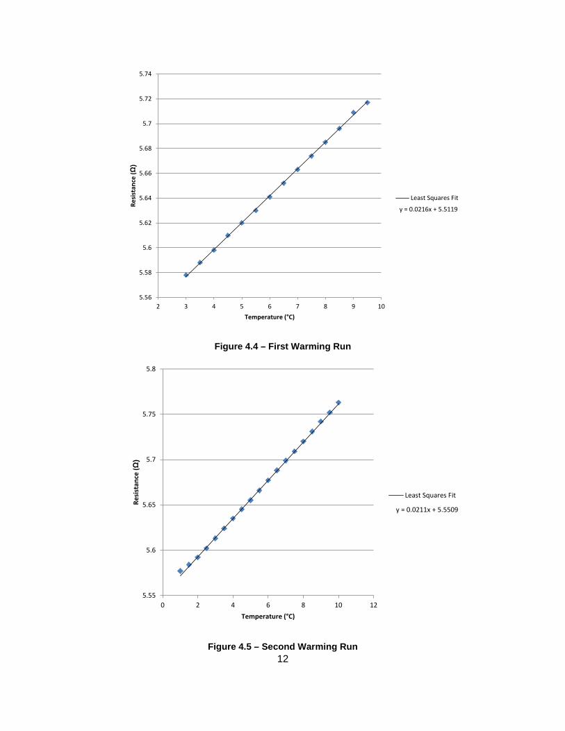
Graphs were plotted of the results, Figures 4.1, 4.2 and 4.3 being those of cooling water and Figures 4.4, 4.5 and 4.6 those of warming water (i.e. from below room temperature). The results obtained showed a high degree of consistency and can be found in section 5.1. The original experimental data can be found in Appendix 1.

Figure 4.1 – First Cooling Run

y = 0.0206x + 5.5228

5.9

6

6.1

6.2

6.3

6.4

6.5

6.6

20 25 30 35 40 45 50

Resi

stan

ce (Ω

)

Temperature (°C)

Least Squares Fit

11

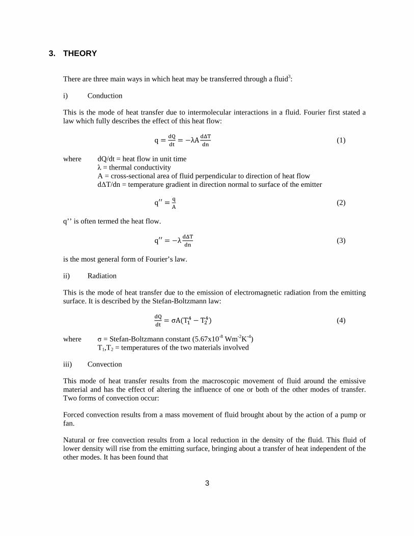
Figure 4.2 – Second Cooling Run

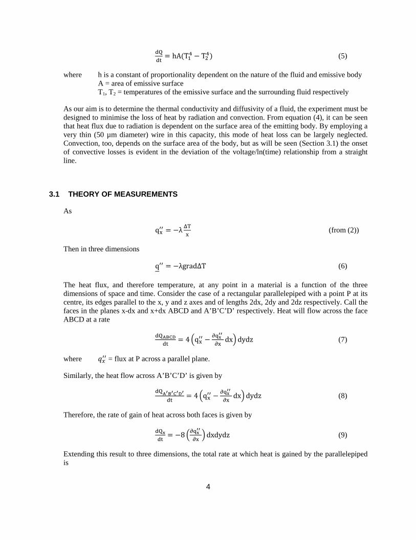
Figure 4.3 – Third Cooling Run

y = 0.0212x + 5.5531

6.05

6.1

6.15

6.2

6.25

6.3

6.35

6.4

6.45

6.5

6.55

6.6

25 30 35 40 45 50

Resi

stan

ce (Ω

)

Temperature (°C)

Least Squares Fit

y = 0.0211x + 5.5627

6.1

6.15

6.2

6.25

6.3

6.35

6.4

6.45

6.5

25 30 35 40 45

Resi

stan

ce (Ω

)

Temperature (°C)

Least Squares Fit

12

Figure 4.4 – First Warming Run

Figure 4.5 – Second Warming Run

y = 0.0216x + 5.5119

5.56

5.58

5.6

5.62

5.64

5.66

5.68

5.7

5.72

5.74

2 3 4 5 6 7 8 9 10

Resi

stan

ce (Ω

)

Temperature (°C)

Least Squares Fit

y = 0.0211x + 5.5509

5.55

5.6

5.65

5.7

5.75

5.8

0 2 4 6 8 10 12

Resi

stan

ce (Ω

)

Temperature (°C)

Least Squares Fit

13

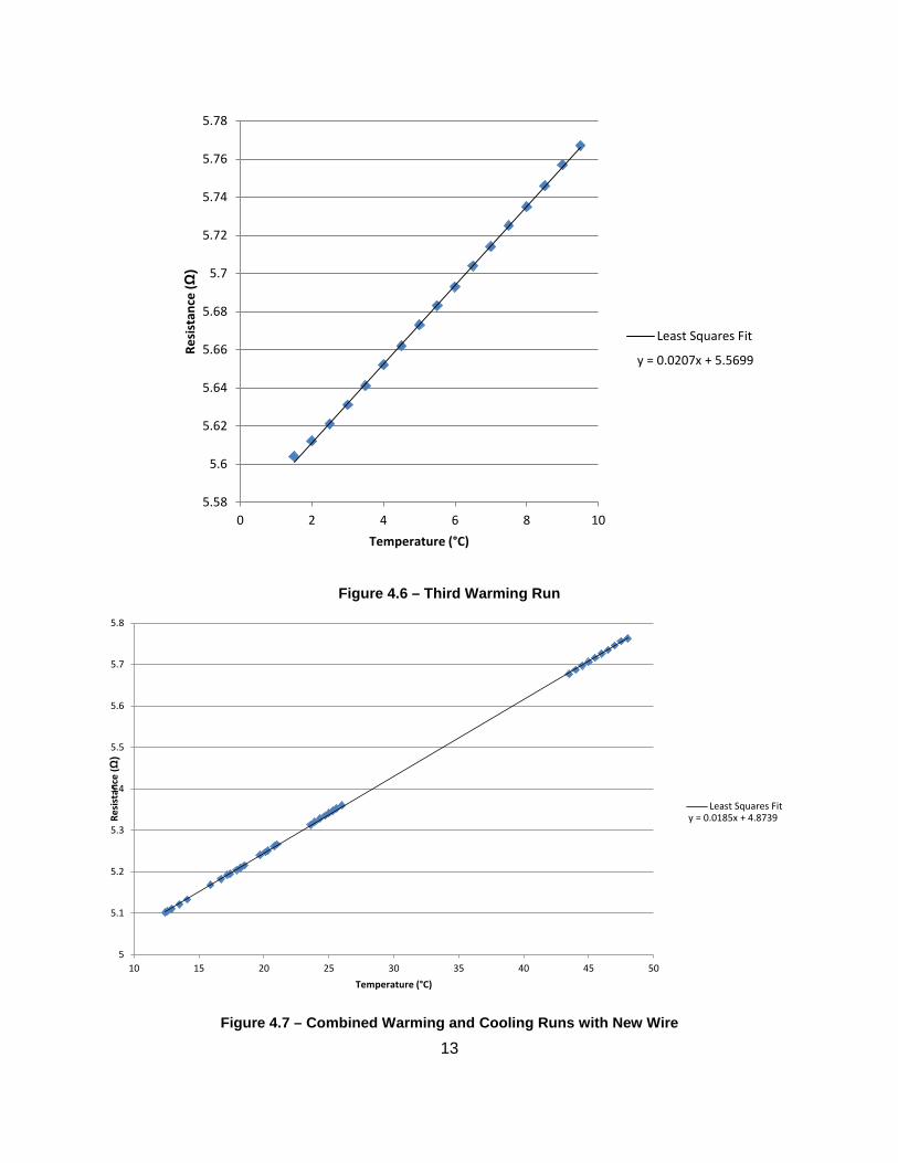
Figure 4.6 – Third Warming Run

Figure 4.7 – Combined Warming and Cooling Runs with New Wire

y = 0.0207x + 5.5699

5.58

5.6

5.62

5.64

5.66

5.68

5.7

5.72

5.74

5.76

5.78

0 2 4 6 8 10

Resi

stan

ce (Ω

)

Temperature (°C)

Least Squares Fit

y = 0.0185x + 4.8739

5

5.1

5.2

5.3

5.4

5.5

5.6

5.7

5.8

10 15 20 25 30 35 40 45 50

Resi

stan

ce (Ω

)

Temperature (°C)

Least Squares Fit

14

Concerns were raised at this stage that the wire may have been soldered to the mounting in the test chamber incorrectly, resulting in a dry joint. When a new wire was fitted, the change of resistance with temperature was investigated – the result of this test is in Figure 4.7. This new wire was used to make the measurements of ΔR versus ln(time) for the remainder of the project.

4.2 APPLICATION OF THE SUPPLIED TEST EQUIPMENT

It was necessary to write driver software for the test box, following the instructions given in reference 6. This was written in Turbo Pascal, this being the only compiled language available, and having sufficient graphics facilities for the needs of the project.

The test box itself caused a few problems – the 50-way “D”-type connection from the box to the PC30AT board was a female type, but male was required. A suitable connector was soon fitted. It was then found that the 4-way connections to the platinum wire had been connected to the wrong pins of its 9-way connector. Once discovered, this was soon rectified. After further problems with obtaining meaningful results, it was found that the polarity of the operational amplifier in the test box had been changed since the original instruction sheet had been written. It was then found necessary to alter the value of a resistance in the test box, as it had originally been intended to use a 25µm diameter wire (resistance ~25Ω) whereas a 50µm diameter wire (resistance 5.2Ω) was actually used. Once these initial teething troubles had been overcome, progress in making meaningful measurements was quickly made – raw data was obtained and a graph-plotting procedure was developed. This was further refined so that it was possible to exaggerate the vertical scale, so that once found, the section of interest could be examined more carefully. It was then possible to make approximate measurements from the monitor screen, printed screen dumps or by reference to the X and Y values of sample points in the section of interest. The vertical scale was altered to read first in volts, then in ohms, rather than the arbitrary units used by the test box. It was found that the wire’s container had to be kept as immobile in order to avoid forced convection due to vibration.

An attempt was made to sample in the ln(time) domain, i.e. taking readings more frequently early on in the experiment and less frequently later on, as convection set in. It was decided that a constant sampling rate (10Hz) yielded sufficient sample values in the required area. Problems were found with obtaining exact timing of sampling – this was eventually overcome by utilising timers on the PC30AT board, the PC’s own timer proving inadequate for the task.

15

5. RESULTS

5.1 MEASUREMENTS OF VARIATION OF RESISTANCE WITH TEMPERATURE

Six sets of measurements were made, three for cooling and three for warming (to room temperature). As can be seen from the graphs (following pages) some sample points show a slight deviation from an otherwise straight line, usually at the “end” where measurements began. It is believed that these are not valid points, as it is unlikely that an even temperature would have been reached in the short time that those particular measurements were made.

The values of (dR/dT) derived from the graphs by the method of least squares are as follows:

Figure 4.1 => 0.0206 Ω/°C Figure 4.2 => 0.0212 Ω/°C Figure 4.3 => 0.0211 Ω/°C Figure 4.4 => 0.0216 Ω/°C Figure 4.5 => 0.0211 Ω/°C Figure 4.6 => 0.0207 Ω/°C

The mean of these results is 0.0211 Ω/°C

An estimate of the error involved is therefore

(1 – (0.0211/0.0206)) x 100% ≈ 2.5%

so

δ(dR/dT)/(dR/dT) ≈ 0.025

The new wire was similarly tested – the results may be seen in Figure 4.7. By the method of least squares, dR/dT was found to be 0.0185 Ω/°C.

5.2 MEASUREMENTS OF RESISTANCE CHANGE AND LN(TIME)

A value of dΔR/dln(t), from a curve fitted to the data is 0.00712 Ω/ln(s), however, this was obtained before accurate sample timing had been achieved. The screen dumps taken after timing correction gave values of dΔR/dln(t) of 0.0075 Ω/ln(s).

From equation (29):

λ = I2R4πL

× dRd∆T

× d(ln (t))dR

where dR/dΔT = gradient of graph from section 5.1 = 0.0185 Ω/°C I = 0.238 A R = 5.3 Ω

16

L = 0.099 m d(ln(t))/dR = reciprocal of gradient of graph from section 5.2 = 200/1.5 = 133.33 ln(s)/Ω

gives a value for thermal conductivity λ for water at 20°C of

λwater = 0.596 (to 3 decimal places)

being a -0.3% difference from the expected value at 20°C (approximately 0.598).

Thermal diffusivity Κ is given by equation (14), thus given values of density and specific heat capacity of water at 20°C of

ρ = 998.21 kg/m3

cp = 4181.8 J/kg °C

then

Κwater = 1.43 x 10-7 m2/s

which is a 4% difference from the expected value at 20°C (approximately 1.49 x 10-7 m2/s).

5.2.1 Error Calculation

The total error in the experiment is given by the sum of the errors in 2I, R, L, dΔT and d(ln(t)):

2δI/I = 0.02/0.25 = ±8x10-3

δR/R = 0.2/4.9 = ±0.04

δL/L = 0.002/0.099 = ±0.02

As dΔT = µdΔR,

error in dΔT = error in µ + error in dΔR = ±0.05

δd(ln(t))/d(ln(t)) = 2/100 = ±0.02

Total error budget = ±14%

The experimental results show an error of -0.3% for thermal conductivity and -4% for thermal diffusivity, so our calculation of ±14% puts our values near the true figure – the best which can be expected at this stage in testing. The timing must be done accurately to ensure accurate results.

17

6. CONCLUSION

The project was successful in its aim of verifying that the test box circuitry was capable of producing results which gave accurate values for the thermal properties of water, giving confidence that the method and proposed circuitry (suitably ruggedized) would be capable of similar performance on the surface of Titan. The circuit, the model for the one to be flown with the Surface Science Package, proved stable over a 20-bit range (a greater than expected accuracy). Whether to employ on-board processing to convert time data into logarithmic data, or to send the raw information directly to Earth, remains to be decided. The feasibility of the method has been established.

The graph plotting software must still be refined, perhaps using the refractometry experiment’s software as a model. The method must still be tested with liquids other than water, for example toluene (around room temperature) and eventually liquid methane/ethane mixtures similar to those expected to be found on Titan.

Future experimentation should also consider the effect on accuracy of varying the sampling rate, for although the output of the test box is bandwidth limited to 10Hz, Nyquist’s theorem implies that the maximum amount of accuracy may be obtained by reading this output at 20Hz or greater. It will at least be necessary to ensure a precise sampling rate – it has not so far proved possible to do this reliably in software. Ideally the current flow should also be computer-controlled. It is believed that errors in measurements encountered in this project are largely due to these timing inaccuracies.

18

7. REFERENCES

1. “Simultaneous measurement of the thermal conductivity and the thermal diffusivity of liquids by

the transient hot-wire method”, Y. Nagasaka & A. Nagashima, Rev. Sci. Instrum 52(2), Feb 1981.

2. “Thermal Conductivity of the Titan Ocean – A Feasibility Study”, Stephen Grant, Part IIB project report, Michaelmas and Lent Terms 1989/90.

3. “Heat Transfer”, Bayley, Owen & Turner, ref. QC320 and “Heat Transfer”, Gebhart, ref. QC320.

4. “Conduction of Heat in Solids”, Carslaw & Jaeger, ref. QC321.

5. “Transducers – an introduction to their performance and design”, Neubert H.K. P., ref. QC872.T6.

6. “Instructions for use of SSP thermal sensor test box”. Available from the Space Sciences Laboratory.

7. “Introduction to Pascal, including Turbo Pascal”, Zaks R., ref. QA264.2.P35.

8. Amplicon Liveline PC30AT instruction manual – available from the Space Sciences Laboratory.

9. "A computer-controlled transient needle-probe thermal-conductivity instrument for liquids", Asher, G. B., Sloan, E. D. & Grabowski, M. S., International Journal of Thermophysics, 1986, v7 (2), p285-294.

19

Appendix 1 - Experimental Data

First Cooling Run Second Cooling Run Third Cooling Run

Temperature (°C) Resistance (Ω) Temperature (°C) Resistance (Ω) Temperature (°C) Resistance (Ω) 47 6.485 47 6.551 44 6.49

46.5 6.477 46.5 6.541 43.5 6.482 46 6.468 46 6.532 43 6.472

45.5 6.457 45.5 6.52 42.5 6.462 45 6.449 45 6.51 42 6.451

44.5 6.438 44.5 6.5 41.5 6.439 44 6.429 44 6.49 41 6.429

43.5 6.418 43.5 6.479 40.5 6.418 43 6.409 43 6.468 40 6.407

42.5 6.398 42.5 6.455 39.5 6.396 42 6.389 42 6.444 39 6.386

41.5 6.379 41.5 6.433 38.5 6.376 41 6.369 41 6.423 38 6.365

40.5 6.357 40.5 6.413 37.5 6.355 40 6.347 40 6.402 37 6.345

39.5 6.336 39.5 6.391 36.5 6.334 39 6.326 39 6.381 36 6.324

38.5 6.316 38.5 6.37 35.5 6.313 38 6.305 38 6.36 35 6.302

37.5 6.296 37.5 6.35 34.5 6.292 37 6.285 37 6.339 34 6.281

36.5 6.275 36.5 6.329 33.5 6.271 36 6.265 36 6.318 33 6.26

35.5 6.255 35.5 6.307 32.5 6.25 35 6.245 35 6.297 32 6.24

34.5 6.235 34.5 6.286 31.5 6.228 34 6.223 34 6.276 31 6.217

33.5 6.213 33.5 6.265 30.5 6.206 33 6.203 33 6.255 30 6.196

32.5 6.193 32.5 6.244 29.5 6.185 32 6.182 32 6.233 29 6.175

31.5 6.171 31.5 6.222 28.5 6.165 31 6.162 31 6.212 28 6.155

30.5 6.151 30.5 6.201 27.5 6.144 30 6.14 30 6.19 27 6.133

29.5 6.131 29.5 6.179 26.5 6.122 29 6.12 29 6.169

28.5 6.109 28.5 6.159 28 6.098 28 6.149

27.5 6.088 27.5 6.138 27 6.078 27 6.127

26.5 6.068 26.5 6.116 26 6.057 26 6.106

25.5 6.047 25 6.037

24.5 6.026 24 6.016

23.5 6.006 23 5.995

22.5 5.985

20

First Warming Run Second Warming Run Third Warming Run

Temperature (°C) Resistance (Ω) Temperature (°C) Resistance (Ω) Temperature (°C) Resistance (Ω) 3 5.578 1 5.577 1.5 5.604

3.5 5.588 1.5 5.584 2 5.612 4 5.598 2 5.592 2.5 5.621

4.5 5.61 2.5 5.602 3 5.631 5 5.62 3 5.613 3.5 5.641

5.5 5.63 3.5 5.624 4 5.652 6 5.641 4 5.635 4.5 5.662

6.5 5.652 4.5 5.645 5 5.673 7 5.663 5 5.655 5.5 5.683

7.5 5.674 5.5 5.666 6 5.693 8 5.685 6 5.677 6.5 5.704

8.5 5.696 6.5 5.688 7 5.714 9 5.709 7 5.699 7.5 5.725

9.5 5.717 7.5 5.709 8 5.735 8 5.72 8.5 5.746 8.5 5.731 9 5.757 9 5.742 9.5 5.767 9.5 5.752 10 5.763

21

Combined Warming and Cooling Runs with New Wire

Temperature (°C) Resistance (Ω) 26 5.36

25.6 5.353 25.3 5.347 25 5.341

24.7 5.335 24.3 5.328 23.9 5.32 23.6 5.313 21 5.266

20.8 5.261 20.3 5.251 20.1 5.247 19.7 5.24 13.5 5.121 12.4 5.101 12.6 5.105 12.9 5.11 14.1 5.133 15.9 5.168 16.7 5.182 17.2 5.192 17.4 5.195 17.9 5.204 18.2 5.209 18.5 5.215 48 5.763

47.5 5.756 47 5.746

46.5 5.735 46 5.726

45.5 5.716 45 5.706

44.5 5.697 44 5.687

43.5 5.677