Temporally Constrained Reconstruction Applied to MRITemperature Data

Nick Todd,1,2* Ganesh Adluru,2,3 Allison Payne,4 Edward V.R. DiBella,2 andDennis Parker2

The monitoring of thermal ablation procedures would benefitfrom an acceleration in the rate at which MRI temperature mapsare acquired. Constrained reconstruction techniques havebeen shown to be capable of generating high quality imagesusing only a fraction of the k-space data. Here, we present atemporally constrained reconstruction (TCR) algorithm appliedto proton resonance frequency shift (PRF) data. The algorithmgenerates images from undersampled data by iteratively mini-mizing a cost function. The unique challenges of using an iter-ative constrained reconstruction technique to generate real-time images were addressed. For a set of eight heating exper-iments on ex vivo porcine tissue, a maximum reduction factor of4 was achieved while keeping the root mean square error(RMSE) of the temperature below 0.5°C. For a set of threeheating experiments on in vivo canine muscle tissue, the max-imum reduction factor achieved was 3 while keeping the tem-perature RMSE below 1.0°C. At these reduction factors, theTCR algorithm underpredicted the thermal dose by an aver-age of 6% for the ex vivo data and 28% for the in vivo data.Compared with sliding window and low resolution recon-structions, the RMSE of the TCR algorithm was significantlylower (P < 0.05 in all cases). Magn Reson Med 62:406–419, 2009.© 2009 Wiley-Liss, Inc.

Key words: constrained reconstruction; temperature; protonresonance frequency shift; dose

Minimally invasive thermal therapies are being developedin which radiofrequency currents, microwaves, lasers, orhigh intensity focused ultrasound (HIFU) are used to pref-erentially kill tumor cells (1,2). To improve the safety andefficacy of these treatments, better techniques to monitorthe process must be developed. Temperature changes inthe tumor and the surrounding tissue must be tracked inreal-time to detect the instant attainment of endpoint tem-peratures or to calculate the accumulated thermal dose inthese regions. MRI is capable of detecting changes in tissuedue to heating and is also able to measure temperaturedistributions in a variety of tissue types. Most investigatorsuse the proton resonance frequency (PRF) shift techniqueto monitor heating and thermal dose accumulation duringthermal treatments (3,4). PRF is currently the most accu-rate method for creating temperature maps and can pro-

vide adequate spatial resolution within a single two-di-mensional (2D) image (5). However, the temporal resolu-tion of PRF scans must be improved to provide adequateresolution over a 3D volume with sufficient temporal res-olution to meet the needs of increasingly sophisticatedtumor ablation procedures that incorporate higher energydepositions, real-time feedback control, and offline trajec-tory optimization.

Thermal therapies focus the applied energy on a smallvolume, causing rapid heating and, potentially, rapid doseaccumulation. The thermal dose, which provides a mea-sure of equivalent tissue damage, is given as the cumula-tive effect of temperature over time, as:

D43 � �t�0

t�final

R�43�Tt��t [1]

Where D43 is the equivalent thermal dose at 43°C, R �0.5 is used for T � 43°C, and R � 0.25 is used for T � 43°C(6). Tissue is considered to be fully necrosed when thermaldose has reached 240 cumulative equivalent minutes(CEM) (7). Because thermal dose rate is a nonlinear expo-nential function of temperature, high spatial and temporalresolution in temperature measurements is especially im-portant in the area where the temperature is increasingmost rapidly and to the highest values. HIFU treatmentshave been proposed in which large amounts of ultrasoundpower are deposited quickly to the region of interest, tem-perature information from the MR scan is sent to a con-trolling computer, and the ultrasound power deposition isadjusted according to safety and efficacy concerns (8,9). Intreatments such as these, the ultrasound can induce tem-perature changes in tissue of up to 20°C in under 30 s. Iftissue temperature is at 57°C (20°C above baseline), it willaccumulate dose at a rate of 273 CEM/s. In this environ-ment, to effectively monitor dose and use a feedback loopto control the power deposition appropriately, entire vol-umes need to be scanned in seconds.

The PRF method for creating temperature maps acquiresdata using a fast gradient echo pulse sequence. It has beenshown that the optimal signal to noise ratio (SNR) for thetemperature data occurs when the echo time equals theT2* of the tissue (5). However, selecting the echo time tobe on the order of T2* would make the scan unacceptablylong and, therefore, shorter echo times, generally between5 and 15 ms, are used in practice. As an example, considera 2D, multislice interleaved gradient echo sequence usedat 3 Tesla (T). For an echo time of 10 ms, a 110-ms repe-tition time (TR) could accommodate 8 slices and an imag-ing matrix of 128 � 128 could be acquired in 14 s. The SNRand in plane spatial resolution of such a scan would be

1Department of Physics, University of Utah, Salt Lake City, Utah.2Department of Radiology, University of Utah, Salt Lake City, Utah.3Department of Electrical and Computer Engineering, University of Utah, SaltLake City, Utah.4Department of Mechanical Engineering, University of Utah, Salt Lake City,Utah.*Correspondence to: Nick Todd, UCAIR, Department of Radiology, 729 Arap-een Drive, Salt Lake City, Utah 84108. E-mail: nicktodd99@yahoo.comReceived 2 July 2007; revised 23 December 2008; accepted 9 February 2009.DOI 10.1002/mrm.22012Published online 7 April 2009 in Wiley InterScience (www.interscience.wiley.com).

Magnetic Resonance in Medicine 62:406–419 (2009)

© 2009 Wiley-Liss, Inc. 406

adequate, but the volume coverage would need to be in-creased and the scan time is far too long for high temper-ature (�50°C) MR-guided thermal therapy applications.

Several strategies exist for reducing the scan times of aPRF sequence and each comes with a trade off. Echo-shifted gradient echo imaging has been proposed as a wayto lengthen echo time (TE) times while keeping TR timesshort (10). Using this method, scan times of 3.6 s pervolume have been achieved (11), but the short TR causessubstantially reduced signal in tissues with typically long(1 s) T1 values. Parallel imaging with multiple receivercoils and SENSE (12) or SMASH (13) reconstruction isanother option. For n coils, one can achieve a speed upfactor, R, up to n, but SNR will also decrease by at least afactor of �R. A variety of reduced data reconstructiontechniques have been proposed to decrease the scan timeof dynamic imaging, including UNFOLD (14), k-t BLAST(15), keyhole (16), RIGR (17), and sliding window, but eachhave limitations in SNR, resolution, or require a prioriknowledge about the location of the changing temperature.

Here, we propose Temporally Constrained Reconstruc-tion (TCR), another reduced data scheme in which thereconstruction is dealt with by means of an inverse prob-lem approach with certain application specific constraints.The technique has already been applied as a way of im-proving the temporal resolution of dynamic contrast en-hanced cardiac imaging (18), and is analogous to recenttechniques sometimes termed compressed sensing (19).Reduction factors of five were achieved with Cartesianundersampling, but the reconstruction was done retro-spectively on the entire data set. In contrast, the currentwork shows that TCR can be applied to PRF temperaturedata to produce images in near real-time and achieve datareduction factors of up to 4 (R � 4) without sacrificing SNRor the accuracy of the temperature measurements. Thedecrease in data acquisition can be parlayed into shorterscan times, greater volume coverage, or better spatial res-olution.

METHODS

TCR Theory

When obtaining a set of images over time, the standardreconstruction method is to acquire every line of k-spacefor each time frame (all of k-t space) and apply the inverse2D Fourier Transform to each time frame. If k-space isundersampled for any time frame then aliasing appears inthe reconstructed image of that frame. The TCR techniqueundersamples k-t space but then uses an appropriate tem-poral (TCR) and/or spatial model (STCR) (20) as a con-straint to remove the aliasing artifact through an iterativeminimization process. Undersampling is done in such away that each phase encode line is acquired at some pointin k-t space. For example, if phase encode lines 1, 5, 9, 13,. . . are sampled in the first time frame, then lines 2, 6, 10,14, . . . are sampled in the second time frame, and so on.

Consider a fully sampled k-space data set, d, and anundersampled k-space data set, d. For standard recon-struction, the complex image data, m, would be obtainedusing the discrete inverse Fourier Transform:

m � F�1d [1]

where F�1 is the 2D inverse Fourier Transform. Applyingthe 2D inverse Fourier Transform to undersampledk-space data, d, would create an image data set, m, withaliasing. To resolve this problem and obtain a nonaliasedsolution, m*, a cost function is created and minimized.The terms of the cost function consist of a data fidelityterm, which ensures faithfulness to the originally acquiredsparse data, and a constraint term consisting of a modelthat is appropriate for the application and is satisfied bythe full data. The data fidelity term is:

�WFm̃ � d�22 [2]

Where F is the 2D Fourier transform, W is a binarysparsifying function that represents which phase encodinglines have been acquired, m̃ is the image estimate, and �o�2

represents the L2 norm. The constraint term is:

���m̃� [3]

Here, is any application appropriate operator acting onthe image estimate, m̃, weighted by �. Thus, the cost func-tion that produces m* when minimized becomes:

m* �arg min

m̃ ��WFm̃ � d�22 � ���m̃�� [4]

In this work, the minimization of the cost function is doneusing an iterative gradient descent method (18).

TCR Applied to PRF Temperature Data

Applying this technique to PRF temperature data, wherethe ultimate goal is real-time monitoring of tissue heating,imposes some unique challenges. The most important isthe choice of , the operator that defines the constraintmodel. In this work, two choices were considered. Thefirst is a maximum smoothness in time function given by:

��m̃� � �i

N

��tm̃i�22 [5]

Here the sum is over the N pixels in a time frame, ƒt isthe temporal gradient operator, and m̃i is the ith pixel of theimage estimate over time. This model assumes that nomotion is present and that both the real and imaginaryparts of the image data vary smoothly in time. The use ofthis constraint in the cost function will penalize solutionsthat have sharply varying time curves. The second con-straint considered is based on a total variation in timemodel and is given by:

��m̃� � �i

N

����tm̃i�2 � �2�1 [5A]

In this equation, � is a small positive constant and �o�1

represents the L1 norm. This constraint also imposes apenalty on abrupt changes to the data in time, however,the penalty is not as harsh as the maximum smoothness

TCR of MRI Temperature Data 407

penalty. This constraint will still resolve the aliasing dueto undersampling, but will accommodate actual rapidchanges in time in the real and imaginary image data.

A variable density sampling scheme was chosen for theundersampling. The central eight lines of k-space wereacquired for all times frames. A second region of phaseencode lines, further out in k-space on either side, weresampled not quite as densely and a final region of k-space,furthest from the center, was sampled more sparsely. Inthe second and third regions, the phase encode lines sam-pled were interleaved in time. For example, if one timeframe sampled lines 1, 5, 9, . . .., then the next time framewould sample lines 2, 6, 10,. . .. In this way, all phaseencode lines would be acquired at some point in k-t space.

When this algorithm is applied for reconstructing dy-namic contrast enhanced cardiac imaging, data can beacquired for all time frames and the reconstruction donejointly using the entire time curve for each pixel. This isnot the case when the application is temperature mappingas the images need to be produced and available in real-time. If the images are to be created immediately, then onlythe present and past time frames can be used in the recon-struction algorithm. However, the use of one “future” timeframe in the reconstruction algorithm may significantlyimprove the image quality and temperature accuracy.Adding a “future” time frame will effectively delay theavailability of the images by one acquisition cycle, whichmay be acceptable depending on the application and theextent to which such an addition improves the tempera-ture accuracy.

We have chosen to use sliding window k-space data forthe algorithm initialization. When using the TCR algo-rithm to calculate the final image space data, m*, the initialsliding window k-space data set, d, is comprised of thepresent k-space data and the minimum amount of k-spacedata from previous time frames that is needed to create afull k-space. For example, if time frame 16 is being recon-structed, the k-space data may only contain phase encodelines 4, 8, 12, . . .. In a sliding window initialization, thedata from time frames 15 (which contains phase encodelines 3, 7, 11, . . .), 14 (lines 2, 6, 10, . . .), and 13 (lines 1,5, 9, . . .) would be added to the data from time frame 16.In this way, a full k-space data set is created.

MRI Acquisition and Heating Set Up

All scans were performed on a Siemens TIM Trio 3Tscanner (Siemens Medical Solutions, Erlangen, Germany).A fast spoiled gradient echo sequence was used with thefollowing parameters: TR � 65 ms, TE � 8 ms, five slices(3-mm thickness, 1-mm spacing), flip angle of 20°, and 6/8partial phase Fourier. The imaging matrix size and field ofview varied amongst scans, but were always chosen to givea resolution of approximately 2 � 2 � 4mm3. For a typicalparameter set, the five slices could be acquired in 6.2 s. Allphase encode lines were acquired at each time frame andzeroed out retrospectively to create the undersampled datasets.

Temperature maps were created from all sets of compleximage data by computing the phase angle between pixelsat adjacent time points and then converting the phasedifference, ��, to temperature difference, �T, using therelation (21):

�T ���

��B0TE[6]

Here, TE is the echo time, � is the gyromagnetic ratio, B0

is the main field strength, and for all calculations the valueof the chemical shift coefficient, �, was assumed to be�0.01 ppm/°C (22).

Multiple HIFU heating experiments were performed onex vivo porcine tissue samples and on in vivo caninemuscle, for which IACUC approval was obtained. A 256-element MRI compatible phased-array ultrasound trans-ducer (IGT, Bordeaux, France) was housed in a bath ofdeionized and degassed water with the tissue situatedabove it. An in-house fabricated two-channel surface coilwas positioned just above the sample for better image SNR.The whole unit fit inside the bore of the magnet andheating could be performed simultaneously with MR im-aging with no apparent artifacts. The ultrasound powercould be controlled externally by means of a controllercomputer.

Eleven heating experiments were performed and aregrouped into two categories. The first category consists ofeight experiments that were performed on ex vivo porcinetissue samples. Ultrasound heating was delivered using aconstant power level, either in one approximately 30-sshot, or in multiple shots with long cooling times in be-tween. Images were acquired over the heating phase(s) andthe cooling phase(s). This category of heating experimentis the most basic situation as the sample is relativelyhomogenous and the heating is smooth in time. For thesecond category, three heating experiments were per-formed on in vivo canine muscle. These experiments weremore similar to a realistic ablation experiment in whichthe goal was to produce a visible lesion in the thigh muscleof an anesthetized canine. To achieve this outcome, highultrasound powers were used in a pulsed fashion to in-duce rapid and large temperature changes. The more rapidswitching of the ultrasound power on and off and thehigher powers used created temperature time curves thatchanged more abruptly than those in the porcine tissueexperiments. Additionally, the coil placement was furtherfrom the focal zone, resulting in a lower signal to noiseratio.

Analysis

In optimizing the TCR algorithm, four parameters wereconsidered: the weighting factor, �; the number of itera-tions; the type of constraint; and whether or not to use oneadditional “future” time frame in the algorithm. Optimi-zation was done separately for the two different heatingexperiment categories.

The first step in the optimization process was to deter-mine the optimal �/iteration combination using a training/validation approach. For the ex vivo porcine tissue group,two data sets were used as training and the remaining sixwere used for validation. For the in vivo canine group, onedata set was used for training and two for validation. Foreach experiment group, 4 �/iteration combinations had tobe chosen as there are two constraint types and a decisionwhether or not to use one “future” time frame. The TCRalgorithm was run for each training set with numerous

408 Todd et al.

�/iteration combinations (� from 0.01 to 0.25 for maxi-mum smoothness constraint and from 0.0025 to 0.025 forthe total variation constraint, each with 50, 100, 200, and400 iterations) and a temperature root mean square error(RMSE) was calculated after each run. The region of inter-est (ROI) used for the RMSE calculation covered an areaover the heated region of approximately 12 mm � 20 mmand included all time frames. Temperatures calculatedfrom the full data were used as truth. The lowest RMSE

determined the choice of � and number of iterations. If thetwo training data sets from the ex vivo porcine tissuegroup did not agree on the optimal �/iteration combina-tion, compromise values would be chosen. Additionally,because computation time is a concern, an �/iterationcombination with fewer iterations would be chosen if theRMSE was not degraded by more than 5%.

The next step in the optimization process was to com-pare the four permutations of the algorithm implementa-tion to determine which parameter set performed the best.The �/iteration values chosen by the training data setswere used in the TCR algorithm to reconstruct all valida-tion data sets with all parameter permutations. The voxelswithin the ROIs from all data sets were pooled and a singletemperature RMSE was calculated for each implementa-tion of the algorithm. The Fisher F-test was used to deter-mine whether the TCR algorithm with one parameter setwas significantly better than another.

After the algorithm was fully optimized, it was appliedto the validation data sets at increasing reduction factors todetermine the maximum reduction factor achievable whilekeeping the temperature RMSE over an ROI below a pre-determined level: 0.5°C for the ex vivo porcine tissuegroup and 1.0°C for the noisier in vivo canine group. Thetemperatures reconstructed by the TCR algorithm at themaximum reduction factor were analyzed for significantfeatures that the total RMSE may have masked. For exam-ple, how the algorithm performed when the temperaturewas changing the fastest, or how well it predicted the peaktemperatures.

Finally, the performance of the TCR algorithm wastested against two other more basic reduced data recon-struction methods, sliding window and low resolution.The same experimental data was used for the compari-sons, only the respective k-spaces were constructed dif-ferently. The sliding window k-space was created asdescribed above. For the low resolution reconstructions,the reduction factor determined how many phase en-code lines about the center of k-space would be used andthe rest of k-space was zero filled. For both the slidingwindow and low resolution reconstructions, a standardInverse Fourier Transform was used to create imagesfrom k-space. The comparison across methods again

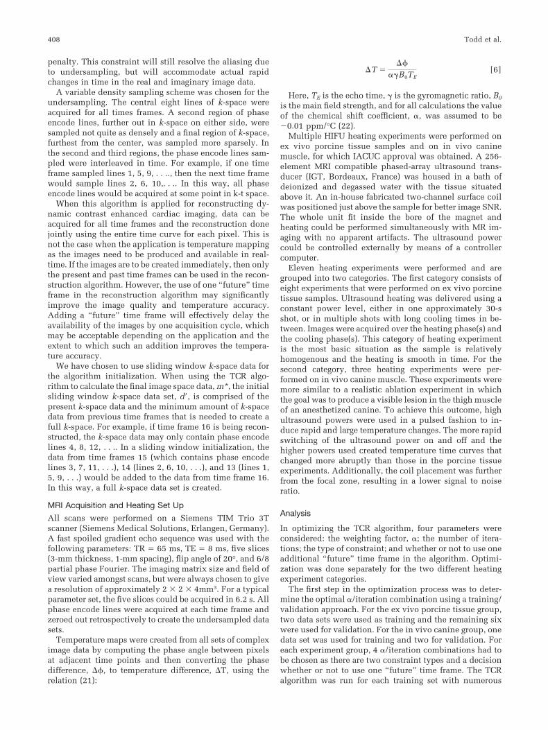
FIG. 1. Determining optimal values for � and number of iterations.a: The temperature RMSE of a single time frame from the first the exvivo porcine training data set as a function of number of iterations.Convergence is almost complete after 100 iterations. b: The tem-perature RMSE for several different �/iteration combinations fromthe same data set.

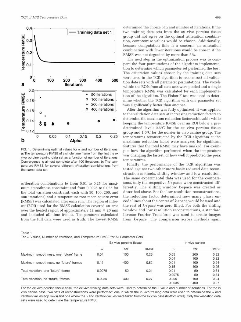
Table 1The � Values, Number of Iterations, and Temperature RMSE for All Parameter Sets

Ex vivo porcine tissue In vivo canine

� iter RMSE � iter RMSE

Maximum smoothness, one ‘future’ frame 0.04 100 0.26 0.05 200 0.820.04 100 0.82

Maximum smoothness, no ‘future’ frames 0.15 400 0.82 0.01 100 0.940.15 400 0.95

Total variation, one ‘future’ frame 0.0075 50 0.21 0.01 50 0.840.0075 50 0.84

Total variation, no ‘future’ frames 0.0035 400 0.27 0.005 100 0.940.0035 400 0.97

For the ex vivo porcine tissue case, the ex vivo training data sets were used to determine the � value and number of iterations. For the invivo canine case, two sets of reconstructions were performed: one in which the in vivo training data were used to determine the � anditeration values (top rows) and one where the � and iteration values were taken from the ex vivo case (bottom rows). Only the validation datasets were used to determine the temperature RMSE.

TCR of MRI Temperature Data 409

used only the validation data sets and the Fisher F-teston the temperature RMSEs.

RESULTS

Optimization

The TCR algorithm was optimized by first determining the�/iteration combination for all four parameter permuta-tions in both heating experiment categories. Consider thecase of the first training data set from the ex vivo porcine

group at a reduction factor of four, using the maximumsmoothness constraint and one “future” time frame. Thebehavior of the temperature RMSE of time frame 20 isplotted against number of iterations in Figure 1A for � �0.05. Beyond 200 iterations, little improvement is seen inthe temperature RMSE. The RMSE values of this data set(now over all 60 time frames) for all �’s at 50, 100, 200, and400 iterations are shown in Figure 1B. The �/iterationcombination that gave the lowest RMSE value was 0.025/400 (RMSE � 0.1322). The trend in the RMSE values forthe second ex vivo porcine training data set was similar,

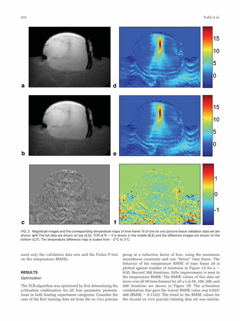
FIG. 2. Magnitude images and the corresponding temperature maps of time frame 16 of one ex vivo porcine tissue validation data set areshown. a–f: The full data are shown on top (A,D), TCR at R � 4 is shown in the middle (B,E) and the difference images are shown on thebottom (C,F). The temperature difference map is scaled from �2°C to 2°C.

410 Todd et al.

although the minimum RMSE value was shifted out to-ward a higher alpha value: 0.20/400 (RMSE � 0.3169). Forthe two training data sets, using the optimal � at 100iterations only degraded the temperature RMSE by 1.0%and 4.0%, respectively. Therefore, the number of itera-tions was set to 100 and a compromise value of � � 0.04was chosen. The �/iteration combinations for the remain-ing permutations of algorithm parameters and the in vivocanine group were chosen in a similar fashion. The resultsare summarized in Table 1.

Using the �/iteration combinations determined by thetraining data sets, the TCR algorithm was run to recon-struct the validation data sets in each experiment categoryfor all parameter permutations (constraint type andwhether or not to use one “future” time frame). Tempera-ture RMSEs were calculated from the pooled voxels of allvalidation data sets for each category. The results areshown in Table 1. Two sets of results are shown for the invivo canine experiments. In the top row, the � and itera-tion values were determined from the in vivo training dataset. In the bottom row, the � and iteration values are thosethat were determined by the ex vivo training data sets. Thetop row RMSE results were used when comparing thedifferent algorithm implementations for significant differ-ences. For both experiment categories, the use of one “fu-

ture” time frame in the reconstruction with a given con-straint type led to significantly improved RMSE values(P � 0.05 for each). The total variation constraint per-formed significantly better than the maximum smoothnessconstraint in the ex vivo porcine tissue experiment cate-gory, but not in the in vivo canine category. The totalvariation constraint with one “future” time frame waschosen as the optimal parameter set because it requiredfewer iterations to converge. It should be noted that ifusing one “future” time frame in the reconstruction is notacceptable for a particular application, then the total vari-ation constraint outperforms the maximum smoothnessconstraint significantly in the case the of ex vivo porcinetissue experiments (P � 0.05) but not in the case of the invivo canine experiments.

Maximum Reduction Factor

Using the optimized parameters of � � 0.0075, 50 itera-tions, the total variation constraint and the one “future”time frame in the TCR algorithm, the largest reductionfactor achieved while keeping the temperature RMSE be-low 0.5°C was R � 4 for the ex vivo porcine tissue exper-iment data sets. Magnitude images and temperature mapsfrom time frame 16 of a validation data set are shown in

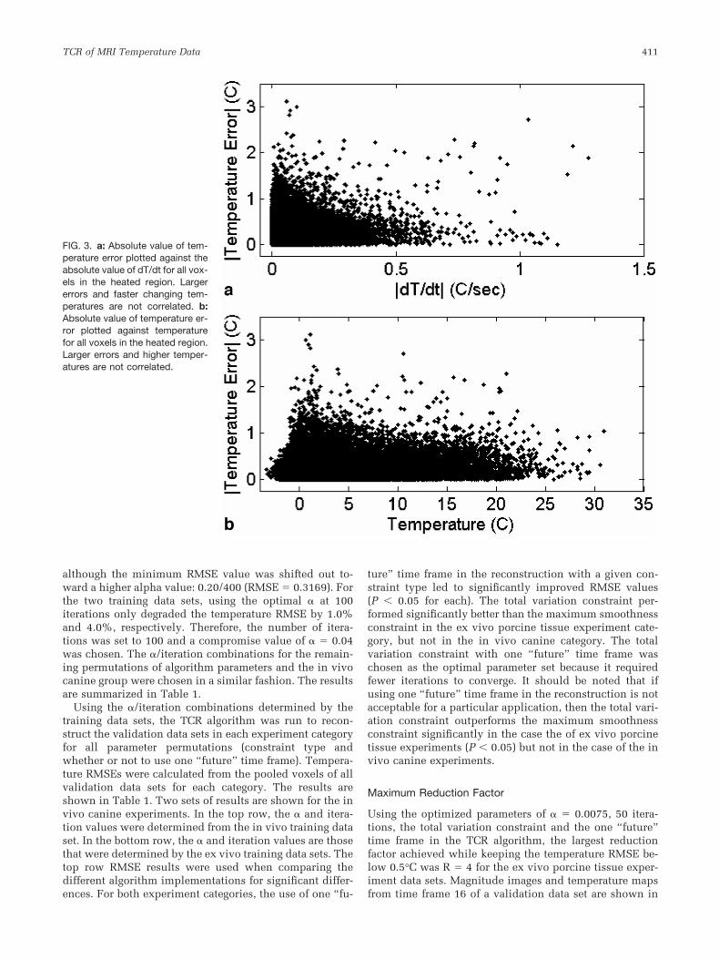
FIG. 3. a: Absolute value of tem-perature error plotted against theabsolute value of dT/dt for all vox-els in the heated region. Largererrors and faster changing tem-peratures are not correlated. b:Absolute value of temperature er-ror plotted against temperaturefor all voxels in the heated region.Larger errors and higher temper-atures are not correlated.

TCR of MRI Temperature Data 411

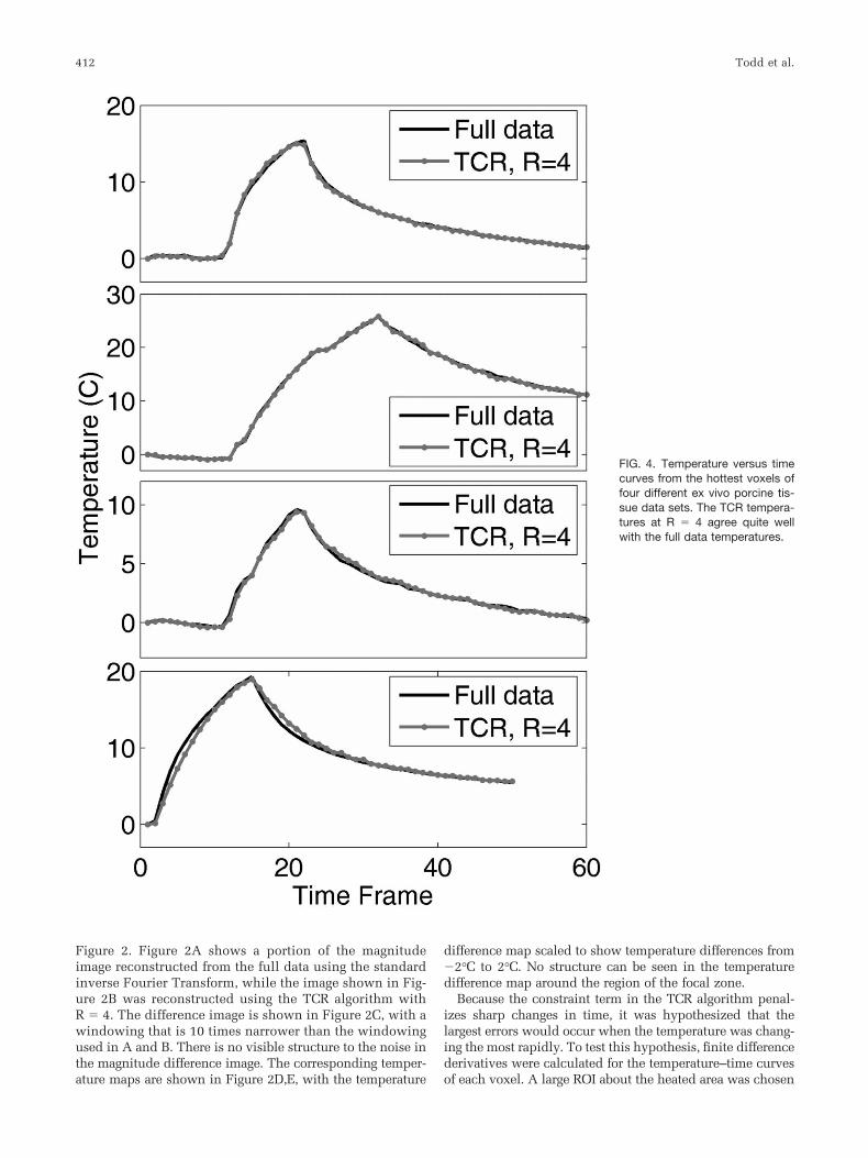
Figure 2. Figure 2A shows a portion of the magnitudeimage reconstructed from the full data using the standardinverse Fourier Transform, while the image shown in Fig-ure 2B was reconstructed using the TCR algorithm withR � 4. The difference image is shown in Figure 2C, with awindowing that is 10 times narrower than the windowingused in A and B. There is no visible structure to the noise inthe magnitude difference image. The corresponding temper-ature maps are shown in Figure 2D,E, with the temperature

difference map scaled to show temperature differences from�2°C to 2°C. No structure can be seen in the temperaturedifference map around the region of the focal zone.

Because the constraint term in the TCR algorithm penal-izes sharp changes in time, it was hypothesized that thelargest errors would occur when the temperature was chang-ing the most rapidly. To test this hypothesis, finite differencederivatives were calculated for the temperature–time curvesof each voxel. A large ROI about the heated area was chosen

FIG. 4. Temperature versus timecurves from the hottest voxels offour different ex vivo porcine tis-sue data sets. The TCR tempera-tures at R � 4 agree quite wellwith the full data temperatures.

412 Todd et al.

and the absolute value of the temperature error of every voxelwas plotted against the absolute value of its time derivative.This scatter plot, containing data from all six ex vivo porcinetissue validation data sets, is shown in Figure 3A. Contrary tothe hypothesis, larger errors and faster changing tempera-tures are not correlated. Also of interest is the behavior of thealgorithm as a function of temperature. A second scatter plot,shown in Figure 3B, shows the absolute value of the errorplotted against temperature over the same ROI. The algo-rithms performance seems to be independent of temperature.

Four representative temperature versus time curves areshown in Figure 4. Each plot is of the voxel within theultrasound focal zone that had the largest temperaturechange. The curve in Figure 4A is from the first trainingdata set and the curves in Figure 4B–D are from validationdata sets. The black lines show the temperatures calcu-lated from the full data while the red lines show thetemperatures calculated using TCR with R � 4. In eachcase, the TCR temperatures do not deviate significantlyfrom the full data temperatures. Even at times when the

ultrasound power is turned on or off and the temperatureschange abruptly, the TCR algorithm can handle thesesharp changes. Although, the TCR temperatures plotted inFigure 4D do lag behind the full data temperatures slightlyduring heating and cooling. Also important to note is theability of the TCR algorithm to accurately predict peaktemperatures.

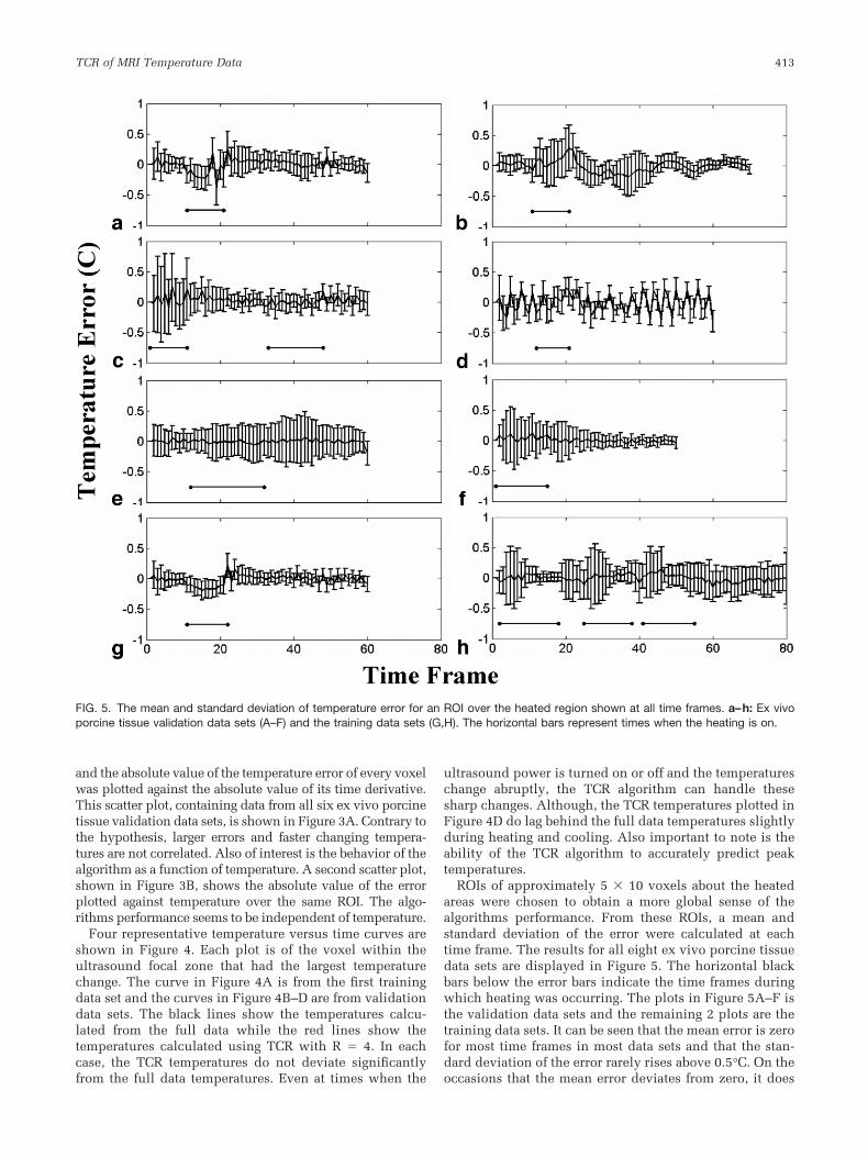
ROIs of approximately 5 � 10 voxels about the heatedareas were chosen to obtain a more global sense of thealgorithms performance. From these ROIs, a mean andstandard deviation of the error were calculated at eachtime frame. The results for all eight ex vivo porcine tissuedata sets are displayed in Figure 5. The horizontal blackbars below the error bars indicate the time frames duringwhich heating was occurring. The plots in Figure 5A–F isthe validation data sets and the remaining 2 plots are thetraining data sets. It can be seen that the mean error is zerofor most time frames in most data sets and that the stan-dard deviation of the error rarely rises above 0.5°C. On theoccasions that the mean error deviates from zero, it does

FIG. 5. The mean and standard deviation of temperature error for an ROI over the heated region shown at all time frames. a–h: Ex vivoporcine tissue validation data sets (A–F) and the training data sets (G,H). The horizontal bars represent times when the heating is on.

TCR of MRI Temperature Data 413

not differ by more than � 0.25°C. The one somewhatanomalous data set is the one shown in Figure 5D, as itexhibits peculiar periodic behavior. An artifact from thepulse sequence must have been present as the magnitudesignal of this data set showed periodic fluctuations on theorder of 5% in the nonheated region of the porcine tissue.

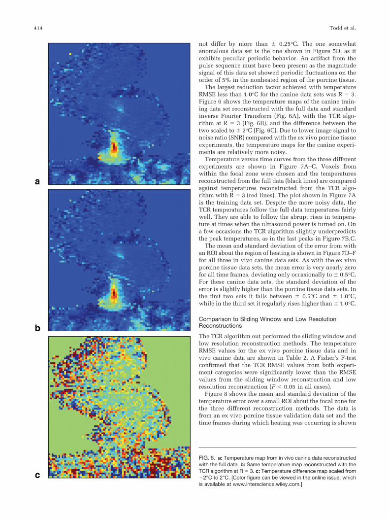
The largest reduction factor achieved with temperatureRMSE less than 1.0°C for the canine data sets was R � 3.Figure 6 shows the temperature maps of the canine train-ing data set reconstructed with the full data and standardinverse Fourier Transform (Fig. 6A), with the TCR algo-rithm at R � 3 (Fig. 6B), and the difference between thetwo scaled to � 2°C (Fig. 6C). Due to lower image signal tonoise ratio (SNR) compared with the ex vivo porcine tissueexperiments, the temperature maps for the canine experi-ments are relatively more noisy.

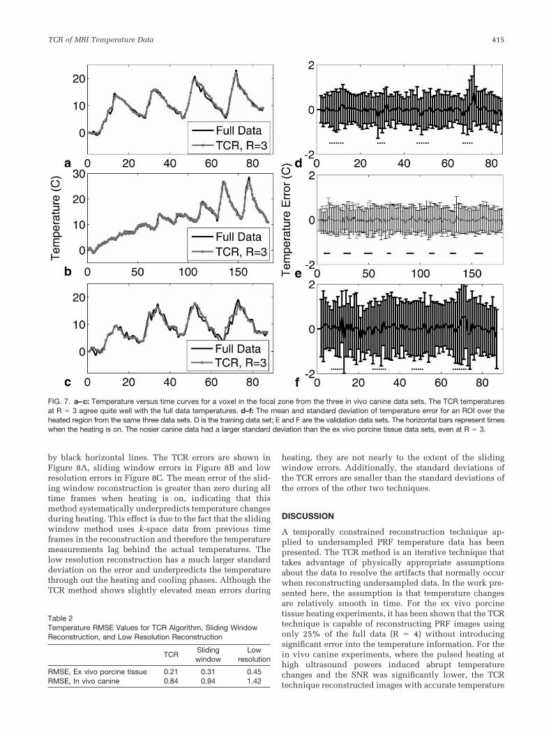
Temperature versus time curves from the three differentexperiments are shown in Figure 7A–C. Voxels fromwithin the focal zone were chosen and the temperaturesreconstructed from the full data (black lines) are comparedagainst temperatures reconstructed from the TCR algo-rithm with R � 3 (red lines). The plot shown in Figure 7Ais the training data set. Despite the more noisy data, theTCR temperatures follow the full data temperatures fairlywell. They are able to follow the abrupt rises in tempera-ture at times when the ultrasound power is turned on. Ona few occasions the TCR algorithm slightly underpredictsthe peak temperatures, as in the last peaks in Figure 7B,C.

The mean and standard deviation of the error from withan ROI about the region of heating is shown in Figure 7D–Ffor all three in vivo canine data sets. As with the ex vivoporcine tissue data sets, the mean error is very nearly zerofor all time frames, deviating only occasionally to � 0.5°C.For these canine data sets, the standard deviation of theerror is slightly higher than the porcine tissue data sets. Inthe first two sets it falls between � 0.5°C and � 1.0°C,while in the third set it regularly rises higher than � 1.0°C.

Comparison to Sliding Window and Low ResolutionReconstructions

The TCR algorithm out performed the sliding window andlow resolution reconstruction methods. The temperatureRMSE values for the ex vivo porcine tissue data and invivo canine data are shown in Table 2. A Fisher’s F-testconfirmed that the TCR RMSE values from both experi-ment categories were significantly lower than the RMSEvalues from the sliding window reconstruction and lowresolution reconstruction (P � 0.05 in all cases).

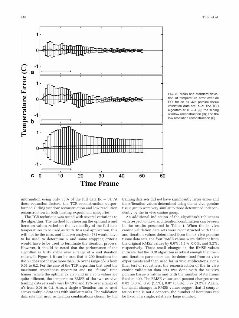
Figure 8 shows the mean and standard deviation of thetemperature error over a small ROI about the focal zone forthe three different reconstruction methods. The data isfrom an ex vivo porcine tissue validation data set and thetime frames during which heating was occurring is shown

FIG. 6. a: Temperature map from in vivo canine data reconstructedwith the full data. b: Same temperature map reconstructed with theTCR algorithm at R � 3. c: Temperature difference map scaled from�2°C to 2°C. [Color figure can be viewed in the online issue, whichis available at www.interscience.wiley.com.]

414 Todd et al.

by black horizontal lines. The TCR errors are shown inFigure 8A, sliding window errors in Figure 8B and lowresolution errors in Figure 8C. The mean error of the slid-ing window reconstruction is greater than zero during alltime frames when heating is on, indicating that thismethod systematically underpredicts temperature changesduring heating. This effect is due to the fact that the slidingwindow method uses k-space data from previous timeframes in the reconstruction and therefore the temperaturemeasurements lag behind the actual temperatures. Thelow resolution reconstruction has a much larger standarddeviation on the error and underpredicts the temperaturethrough out the heating and cooling phases. Although theTCR method shows slightly elevated mean errors during

heating, they are not nearly to the extent of the slidingwindow errors. Additionally, the standard deviations ofthe TCR errors are smaller than the standard deviations ofthe errors of the other two techniques.

DISCUSSION

A temporally constrained reconstruction technique ap-plied to undersampled PRF temperature data has beenpresented. The TCR method is an iterative technique thattakes advantage of physically appropriate assumptionsabout the data to resolve the artifacts that normally occurwhen reconstructing undersampled data. In the work pre-sented here, the assumption is that temperature changesare relatively smooth in time. For the ex vivo porcinetissue heating experiments, it has been shown that the TCRtechnique is capable of reconstructing PRF images usingonly 25% of the full data (R � 4) without introducingsignificant error into the temperature information. For thein vivo canine experiments, where the pulsed heating athigh ultrasound powers induced abrupt temperaturechanges and the SNR was significantly lower, the TCRtechnique reconstructed images with accurate temperature

FIG. 7. a–c: Temperature versus time curves for a voxel in the focal zone from the three in vivo canine data sets. The TCR temperaturesat R � 3 agree quite well with the full data temperatures. d–f: The mean and standard deviation of temperature error for an ROI over theheated region from the same three data sets. D is the training data set; E and F are the validation data sets. The horizontal bars represent timeswhen the heating is on. The nosier canine data had a larger standard deviation than the ex vivo porcine tissue data sets, even at R � 3.

Table 2Temperature RMSE Values for TCR Algorithm, Sliding WindowReconstruction, and Low Resolution Reconstruction

TCRSlidingwindow

Lowresolution

RMSE, Ex vivo porcine tissue 0.21 0.31 0.45RMSE, In vivo canine 0.84 0.94 1.42

TCR of MRI Temperature Data 415

information using only 33% of the full data (R � 3). Atthese reduction factors, the TCR reconstruction outper-formed sliding window reconstruction and low resolutionreconstruction in both heating experiment categories.

The TCR technique was tested with several variations tothe algorithm. The method for choosing the optimal � anditeration values relied on the availability of the full datatemperatures to be used as truth. In a real application, thiswill not be the case, and L-curve analysis (18) would haveto be used to determine � and some stopping criteriawould have to be used to terminate the iteration process.However, it should be noted that the performance of thealgorithm is fairly stable over a range of � and iterationvalues. In Figure 1 it can be seen that at 200 iterations theRMSE does not change more than 5% over a range of �’s from0.01 to 0.2. For the case of the TCR algorithm that used themaximum smoothness constraint and no “future” timeframes, where the optimal ex vivo and in vivo � values arequite different, the temperature RMSE of the two ex vivotraining data sets only vary by 13% and 12% over a range of�’s from 0.01 to 0.2. Also, a single �/iteration can be usedacross multiple data sets with similar results. The validationdata sets that used �/iteration combinations chosen by the

training data sets did not have significantly larger errors andthe �/iteration values determined using the ex vivo porcinetissue group were very similar to those determined indepen-dently by the in vivo canine group.

An additional indication of the algorithm’s robustnesswith respect to the � and iteration combination can be seenin the results presented in Table 1. When the in vivocanine validation data sets were reconstructed with the �and iteration values determined from the ex vivo porcinetissue data sets, the four RMSE values were different fromthe original RMSE values by 0.0%, 1.1%, 0.0%, and 3.2%,respectively. These small changes in the RMSE valuesindicate that the TCR algorithm is robust enough that the �and iteration parameters can be determined from ex vivoexperiments and then used for in vivo applications. For afinal test of robustness, the reconstruction of the in vivocanine validation data sets was done with the ex vivoporcine tissue � values and with the number of iterationsfixed at 400. The RMSE values and percent changes were:0.82 (0.0%), 0.95 (1.1%), 0.87 (3.6%), 0.97 (3.2%). Again,the small changes in RMSE values suggest that if compu-tation time is not a concern, the number of iterations canbe fixed at a single, relatively large number.

FIG. 8. Mean and standard devia-tion of temperature error over anROI for an ex vivo porcine tissuevalidation data set. a–c: The TCRalgorithm at R � 4 (A); the slidingwindow reconstruction (B); and thelow resolution reconstruction (C).

416 Todd et al.

The TCR technique does not use any coil sensitivityinformation and could be used in conjunction with paral-lel imaging methods for even larger reduction factors. Thedata presented here was taken from one channel of atwo-channel receive coil (the channel with the higher SNRwas chosen). While parallel imaging methods produce im-ages with reduced SNR, the TCR technique was found tonot degrade the SNR of its reconstructed image. This find-ing is largely due to the fact that the algorithm smoothesthe data in time and thus signal fluctuations in temporally-adjacent images are reduced.

MR images can be used to monitor thermal therapies inseveral different ways. Modifications to the heating depo-sition can be made by a clinician or a controlling computerand such modifications can be based on either an endpoint temperature or an accumulated dose. It has been

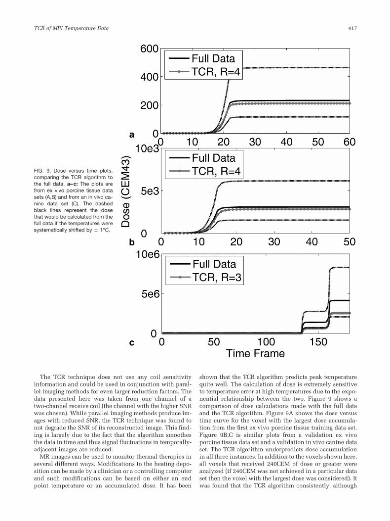
shown that the TCR algorithm predicts peak temperaturequite well. The calculation of dose is extremely sensitiveto temperature error at high temperatures due to the expo-nential relationship between the two. Figure 9 shows acomparison of dose calculations made with the full dataand the TCR algorithm. Figure 9A shows the dose versustime curve for the voxel with the largest dose accumula-tion from the first ex vivo porcine tissue training data set.Figure 9B,C is similar plots from a validation ex vivoporcine tissue data set and a validation in vivo canine dataset. The TCR algorithm underpredicts dose accumulationin all three instances. In addition to the voxels shown here,all voxels that received 240CEM of dose or greater wereanalyzed (if 240CEM was not achieved in a particular dataset then the voxel with the largest dose was considered). Itwas found that the TCR algorithm consistently, although

FIG. 9. Dose versus time plots,comparing the TCR algorithm tothe full data. a–c: The plots arefrom ex vivo porcine tissue datasets (A,B) and from an in vivo ca-nine data set (C). The dashedblack lines represent the dosethat would be calculated from thefull data if the temperatures weresystematically shifted by � 1°C.

TCR of MRI Temperature Data 417

not always, underpredicted the thermal dose. Over all ofthese voxels, the average dose error was �6.3% for the exvivo porcine tissue data sets and �28% for the in vivocanine data sets. The reason for these underestimations isthat the constraint term in the TCR algorithm penalizesabrupt changes in time, causing the reconstructed temper-atures to sometimes fall short at sharp peaks. This subtlesmoothing of the temperature curves can be seen in the lastpeak of the temperature plot in Figure 7B. To put theseerrors into perspective, dashed black lines are shown onthe plots in Figure 9 that represent the dose accumulationthat would be calculated from the full data temperatures ifthere were a systematic temperature offset of �1°C or�1°C. This type of offset could occur, for example, if thesubject body temperature was actually 38°C when it wasassumed to be 37°C. Seen in this light, the TCR errors incalculating dose are reasonable.

In its current form, the computation time for the TCRalgorithm is still too long for real-time image acquisi-tion. In a Matlab (The Mathworks, Natick, MA) imple-mentation on a desktop PC, it takes approximately 5.7 sto reconstruct one slice using the total variation con-straint and 50 iterations. Considering that 5 to 10 sliceswill have to be reconstructed in 1 or 2 s, the computa-tion time will have to be improved by a factor of be-tween 15 and 115. Several ideas will enable the reduc-tion of the computation time to reach real-time. Whenpassing the k-space data into the algorithm, one needonly use a small number of data points in the readoutdirection, keeping only the central portion of the imagewhere the heating is being monitored. This will notaccelerate scan time at all, but it will reduce the size ofthe data matrix that goes into the reconstruction algo-rithm and lessen the computation burden. For all datasets, a quarter of the read out data was sufficient to stillvisualize the entire heated area. There will be no reduc-tion in image resolution and because the entire readoutdata will have been acquired, it can be reconstructedretrospectively if necessary. Cutting the data matrix by afactor of four in the readout direction led to a four-foldacceleration in the TCR algorithm. If some temperatureaccuracy can be sacrificed, then it would be possible touse the algorithm with a constraint weighting term thathas been optimized for fewer iterations. Finally, an ef-ficient C�� implementation on a more powerful com-puter that uses a conjugate gradient method to minimizethe cost function, instead of the currently used gradientdescent technique, will provide additional improve-ment in computation time. Recently published papershave shown that computationally intensive medical im-aging tasks can be processed on a graphics processingunit (GPU) to increase computation speed by factors of85 to 100 (23,24). On such a computer or other parallelcomputing platforms, real-time implementation wouldbe feasible.

Even greater reduction factors should be attainable withmore sophisticated constraint terms. Several investigatorshave shown reconstruction is possible using total variation inspace as a constraint (25). These could be used in addition tothe temporal constraint that is already implemented. Webelieve that information about tissue heating could also be

incorporated into the constraint term. Heating start and stoptimes as well as ultrasound power will be known during anythermal treatment and the temperature evolution within thetissue will follow the Pennes bioheat equation. Using this apriori information to predict how the temperature, and thusthe image phase, will behave could prove to be very useful inthe reconstruction algorithm.

ACKNOWLEDGMENTS

This work has been supported by NIH grants F31 EB007892-01A1 and R01CA087785-04A2, as well as grants from theCumming Foundation, the Ben B. and Iris M. Margolis Foun-dation, and Focused Ultrasound Surgery Foundation.

REFERENCES

1. Bublik M, Sercarz JA, Lufkin RB, Masterman-Smith M, Polyakov M,Paiva PB, Blackwell KE, Castro DJ, Paiva MB. Ultrasound-guided laser-induced thermal therapy of malignant cervical adenopathy. Laryngo-scope 2006;116:1507–1511.

2. Fosse E. Thermal ablation of benign and malignant tumours. MinimInvasive Ther Allied Technol 2006;15:2–3.

3. Carter DL, MacFall JR, Clegg ST, Wan X, Prescott DM, Charles HC,Samulski TV. Magnetic resonance thermometry during hyperthermiafor human high-grade sarcoma. Int J Radiat Oncol Biol Phys 1998;40:815–822.

4. Denis de Senneville B, Quesson B, Moonen CT. Magnetic resonancetemperature imaging. Int J Hyperthermia 2005;21:515–531.

5. Quesson B, de Zwart JA, Moonen CT. Magnetic resonance temperatureimaging for guidance of thermotherapy. J Magn Reson Imaging 2000;12:525–533.

6. Sapareto SA, Dewey WC. Thermal dose determination in cancer ther-apy. Int J Radiat Oncol Biol Phys 1984;10:787–800.

7. Hazle JD, Stafford RJ, Price RE. Magnetic resonance imaging-guidedfocused ultrasound thermal therapy in experimental animal models:correlation of ablation volumes with pathology in rabbit muscle andVX2 tumors. J Magn Reson Imaging 2002;15:185–194.

8. Arora D, Minor MA, Skliar M, Roemer RB. Control of thermal ther-apies with moving power deposition field. Phys Med Biol 2006;51:1201–1219.

9. Arora D, Cooley D, Perry T, Guo J, Richardson A, Moellmer J, Hadley R,Parker D, Skliar M, Roemer RB. MR thermometry-based feedback con-trol of efficacy and safety in minimum-time thermal therapies: phantomand in-vivo evaluations. Int J Hyperthermia 2006;22:29–42.

10. Moonen CT, Liu G, van Gelderen P, Sobering G. A fast gradient-recalledMRI technique with increased sensitivity to dynamic susceptibilityeffects. Magn Reson Med 1992;26:184–189.

11. Mougenot C, Salomir R, Palussiere J, Grenier N, Moonen CT. Automaticspatial and temporal temperature control for MR-guided focused ultra-sound using fast 3D MR thermometry and multispiral trajectory of thefocal point. Magn Reson Med 2004;52:1005–1015.

12. Pruessmann KP, Weiger M, Scheidegger MB, Boesiger P. SENSE: sen-sitivity encoding for fast MRI. Magn Reson Med 1999;42:952–962.

13. Sodickson DK, Manning WJ. Simultaneous acquisition of spatial har-monics (SMASH): fast imaging with radiofrequency coil arrays. MagnReson Med 1997;38:591–603.

14. Madore B, Glover GH, Pelc NJ. Unaliasing by fourier-encoding theoverlaps using the temporal dimension (UNFOLD), applied to cardiacimaging and fMRI. Magn Reson Med 1999;42:813–828.

15. Tsao J, Boesiger P, Pruessmann KP. k-t BLAST and k-t SENSE: dynamicMRI with high frame rate exploiting spatiotemporal correlations. MagnReson Med 2003;50:1031–1042.

16. van Vaals JJ, Brummer ME, Dixon WT, Tuithof HH, Engels H, NelsonRC, Gerety BM, Chezmar JL, den Boer JA. “Keyhole” method for accel-erating imaging of contrast agent uptake. J Magn Reson Imaging 1993;3:671–675.

17. Webb AG, Liang ZP, Magin RL, Lauterbur PC. Applications of reduced-encoding MR imaging with generalized-series reconstruction (RIGR). JMagn Reson Imaging 1993;3:925–928.

418 Todd et al.

18. Adluru G, Awate SP, Tasdizen T, Whitaker RT, Dibella EV. Temporallyconstrained reconstruction of dynamic cardiac perfusion MRI. MagnReson Med 2007;57:1027–1036.

19. Gamper U, Boesiger P, Kozerke S. Compressed sensing in dynamicMRI. Magn Reson Med 2008;59:365–373.

20. Adluru G, Whitaker RT, DiBella VR. Spatio-temporal constrained re-construction of sparse dynamic contrast enhanced radial MRI data. In:Proceedings of the 4th IEEE International Symposium on BiomedicalImaging, Arlington, Virginia, USA, 2007. p 109–112.

21. De Poorter J, De Wagter C, De Deene Y, Thomsen C, Stahlberg F, AchtenE. Noninvasive MRI thermometry with the proton resonance frequency(PRF) method: in vivo results in human muscle. Magn Reson Med1995;33:74–81.

22. Hindman JC. Proton resonance shift of water in the gas and liquidstates. J Chem Phys 1966;44:4582–4592.

23. Hansen MS, Atkinson D, Sorensen TS. Cartesian SENSE and k-t SENSEreconstruction using commodity graphics hardware. Magn Reson Med2008;59:463–468.

24. Sorensen TS, Schaeffter T, Noe K, Hansen MS. Accelerating the non-equispaced fast Fourier transform on commodity graphics hardware.IEEE Trans Med Imaging 2008;27:538–547.

25. Block KT, Uecker M, Frahm J. Undersampled radial MRI with multiplecoils. Iterative image reconstruction using a total variation constraint.Magn Reson Med 2007;57:1086–1098.

TCR of MRI Temperature Data 419