temporal crossover from classical to quantal behavior near dynamical critical points

PHYSICAL REVIEW A VOLUME 36, NUMBER 1 JULY 1, 1987

Temporal crossover from classical to quantal behavior near dynamical critical points

Shmuel FishmanDepartment of Physics, Tech nion Isr—ael Institute of Technology, 32 000 Haifa, Israel

D. R. GrempelInstitut Max Laue —Paul Langeuin, Boite Postale No. 156X, F-38042 Grenoble Cedex, France

R. E. PrangeDepartment of Physics and Center for Theoretical Physics, Uniuersi ty of Maryland, College Park, Maryland 20742

and Institut Max Laue —Paul Langevin, Boite Postale No. 156X, F-38042 Grenoble Cedex, France(Received 3 October 1986)

The behavior of a class of dynamical systems is analyzed as a function of time and of Planck's con-stant A when the latter is small compared with the (classical) action of the system. The case con-sidered is that the classical system (A=O) is near a dynamical critical point, and there is a definitescaling of the variables of the classical motion with time. It is shown that the parameter fi is arelevant variable in the renormalization-group sense, which means that as one scales to longer times,A scales to larger values. This is just a way of saying that quantum effects become progressively moreifnportant with time, and even if they can initially be ignored, there comes a time t* ~A ' ~ afterwhich the system can no longer be treated classically, i.e., t* characterizes the crossover away fromclassical to quantal behavior. This is similar to the effect of noise, which also smears out the deter-ministic classical phase-space path and destroys the sharp stochastic phase transition; however, unlikenoise, the quantum exponent y is simply related to the classical ones. We present arguments thatthis is the consequence of a property of the system's operators in the Heisenberg picture. The casesof a period-doubling cascade to chaos and the disappearance of the last Kol'mogorov-Arnol'd-Mosertrajectory in the standard map are specifically discussed. The results are shown to be consistent withnumerical calculations.

I. INTRODUCTION

The quantum-mechanical behavior of systems that arechaotic in their classical limit has been studied extensivelyin recent years. ' Much of the work in this field is devot-ed to the analysis of statistics of energy levels. It is foundthat for systems with time-independent Hamiltonians,classical chaos is related to level repulsion in the semiclas-sical limit. The classical chaos manifests itself also inirregularities of wave functions and matrix elements.For bounded systems with time-independent Hamiltoni-ans the spectrum is discrete and consequently asymptoti-cally the motion is always quasiperiodic. Therefore, ifone is interested to find chaotic quantum dynamics one isled to study systems with time-dependent Hamiltonians.But also for a class of systems that were studied so far,the classical chaotic behavior is suppressed by quantumeffects. ' The reason is that chaotic classical systemsdevelop during their time evolution complicated structuresin phase space on finer and finer scales. The quantumsystems, on the other hand, cannot have any phase-spacestructure on a scale finer than Planck's constant A. ' 'Consequently, in a quantum system, after some time t'which depends on fz, the classical approximation leadingto a fine scale structure breaks down and there is a cross-over to new quantal behavior. The estimate of the cross-over time to this behavior is one of the main subjects ofthe present work. '

A natural way to study the semiclassical motion of aquantum system is to follow the evolution of a wave pack-et. The Heisenberg uncertainty principle restricts the sizeof the initial packet, and there is a corresponding distribu-tion of classical initial conditions in phase space. In thecase that Planck's constant is small compared with theappropriate classical action, it may be assumed that theinitial packet is well localized in a small part of the avail-able phase space of the system. The wave packet will,however, spread with time. So also will the contributionof the classical distribution of points in phase space.Indeed, for a freely propagating particle, the wave packetspreading is identical to the classical spreading in thelong-time limit. However, in an effectively confinedgeometry (more precisely when the classical motion is ap-propriately nonlinear), there comes a time t* when thewave packet has spread so much that different parts of itinterfere with each other. After that time, the quantalpredictions will differ from the classical ones.

Clearly one expects t* to be a qualitative concept, ascale rather than a precise number. It also can depend onthe initial packet, but much of this dependence is removedby requiring the initial packet to be minimal, and such asto maximize t*. To be precise, one must also replace theloose idea of self-interference of the wave packet by a cri-terion on observable quantities. It is appropriate to studysome general observable, such as the Wigner function,from which other observables may be constructed, and it

36 289 1987 The American Physical Society

290 SHMUEL FISHMAN, D. R. GREMPEL, AND R. E. PRANGE 36

then may happen that the same time t* applies to essen-tially all observables. In an integrable system, nearbypoints in phase space diverge from one another as a powerof the time, for example, linearly. There can be long-timequantum effects, but these will typically appear after atime t* ~A '. The wave packet or classical distributionspreading in a classical chaotic system is much fas-ter, ' ' ' namely exponential in time, since neighboringclassical trajectories diverge as exp(A, ,~t), where A,,~

is theLyapunov exponent. If t* is the time for the wave packetto spread to some fixed size L, e.g. , the size of the system,the relation t* ~in(L/fi)IA, ,, is suggested. However, indriven systems which are unbounded in energy, this maybe too short a time. (Indeed, for the diffusion problemdiscussed below, it has been estimated that t* ~ A in thecase that k„ is large).

It is natural to ask what will be the nature of the cross-over between classical and quantum behavior near criticalpoints of stochastic transitions of the classical systems.Such points are, for example, the accumulation point ofperiod doubling bifurcations ' ' and the destruction ofthe last bounding Kol'mogorov-Arnol'd-Moser (RAM)trajectory of the standard map. ' At this point themap is scale invariant under time rescaling. It is alsouniversal, namely it depends on very few details of the ac-tual system that is studied and large universality classes ofsystems exhibit identical critical behavior. In these as-pects critical points of dynamical systems are similar tosecond-order phase transitions that were analyzed exten-sively by renormalization-group methods. In the vi-

cinity of the phase transition points the effect of small per-turbations can be calculated exploiting the scale invari-ance at the critical point. Such "relevant" perturbationsare, for example, the finite size of the system or an or-dering field ' (like the magnetic field at a ferromagnetictransition) that destroys or rounds the sharp transition.In the present work Planck's constant A plays the role ofthis perturbation. We will show that it is a relevant vari-able which destroys the sharp transition that is found forthe classical system. ' This is also similar to the effect ofnoise on classical systems that exhibit stochastic transi-tions. Noise destroys cycles of long periods and there-fore it removes the sharpness of the transition whereperiods of infinite length are generated. The scaling ofthis destruction is determined by the scaling of the mapwithout noise at the critical point. The effect of quantuminterference is similar and, as it will be seen, it is evensimpler. Although classical noise and quantum interfer-ence similarly affect scaling, their long-time effects arequite different. For example, quantum effects tend tosuppress classical diffusion, while noise always leads tolong-time diffusion, suppressing classical confinement.

The behavior of Hamiltonian classical chaotic systemsthat are relevant for our work is summarized in Sec. II.In Sec. III we develop the equations of motion of thequantum-mechanical operators in the Heisenberg repre-sentation. The scaling of their matrix elements that re-sults from the scaling of the classical maps near their criti-cal points is obtained to the leading order in Planck's con-stant A. In Sec. IV we analyze the scaling of the evolutionoperator of the Wigner function to the leading order in A

using standard semiclassical methods. ' ' In Sec. V wesummarize the physical implications of the scalinganalysis of Secs. III and IV. The main conclusion is thatPlanck's constant A is a relevant variable, in the sense ofthe renorrnalization group. It is related to time by ascaling relationship. For short times classical behaviorholds. For longer times there is a crossover to quan-tal behavior with an exponent that is simply related to theclassical exponents. ' For the kicked rotor it is knownthat classical diffusion ' is suppressed by a mechanismthat is similar to Anderson localization. " ' The scalingtheory that is developed in the present work enables us tofind the crossover exponent between classical diffusionand quantal localization for this system. In Sec. VI somepredictions of the scaling theory are tested numerically forthe kicked rotor and these are found to be consistent withthe numerical data.

II. SCALING OF CLASSICAL SYSTEMSNEAR CRITICAL POINTS

In this section critical properties of maps that are gen-erated by the Hamiltonian

poo

+ V(q) g 6(t —nT)2M

&=—,'p + V(q) g 6(t n) . — (2. 1)

The driving potential V(q) will be specified in what fol-lows, and defines the specific problem that is studied.Note that fi does not explicitly appear in (2.1).

The equations of motion integrated over a period are

qn+1 =q'n+pn ~

p. +i=p. —V'(q. +i»(2.2)

where q„ is the coordinate of the particle at the nth kick,namely at t =n, while p„ is its momentum forn ~ t & n + 1. We denote

will be summarized. Such a Hamiltonian describes a freeparticle that is periodically kicked, where q and p are itsgeneralized coordinate and momentum, respectively. Thefree particle may move in real space and in such a case itscoordinate q will also be denoted by x while p is itsmomentum. We will consider also the planar rotor where

q is an angle variable (denoted by 8) while p is its angularmomentum and M now means the moment of inertia, in-stead of the mass. In derivations that hold for both spa-tial coordinates and angular coordinates the coordinatewill be denoted by q. We now choose the unit of time tobe T and the unit of mass (or moment of inertia) to be M.In the former case, the unit of length X will be chosen sothat the nonlinearity of V(x) is of order unity whenx =X. The natural unit of action is MX T '. The di-mensionless number AT/MX enters the quantum prob-lem. It will be denoted simply by A, since it is in fact thevalue of Planck's constant in the natural units. In theseunits the Hamiltonian becomes

36 TEMPORAL CROSSOVER FROM CLASSICAL TO QUANTAL. . . 291

avV'(q„) ——

qn+) = y—n+F (qn ) ~

y. +) =q. F'(—q. +) )

where

(2.3)

The map can be transformed to the "de Vogelaere"form

are not special to (2.6). Points in phase space that areclose to points of a stable periodic cycle are transformedby the map to points that are close to that cycle. It is ex-pected and found that the scaling of the cycles resultingfrom the geometric convergence (2.8) is satisfied by themap (2.3) near the accumulation point of period-doublingbifurcations. A map T in the plane can be defined for-mally as

z„+,= T (AA, ,z„)

y = —b +-,' V'(q)] (2.4)[T —(b,X,z„),Ty(bÃ, z„)], (2.10)

and

F(q)= —,'[q —V(q)] . (2.5)

The potential V (q ) [and therefore the function F (q) ]determines the nature of the map. A large variety of non-linear maps of the form (2.3) exhibit a cascade of period-doubling bifurcations. A specific map that was extensive-ly studied is the quadratic map ' ' with

T*(b,k, ,z)= lim [A"T' )(5 "bg, A "z)], (2. 1 1)

where

where z„=(x„—x„y„)and b,k=k —A,The functions T and T~ define the map. Such a map

is (2.3), for example. We denote the map applied n timesby T "'. The map satisfies asymptotic scale invariance,namely, there exists a universal map

Fq(x) =M —(1—k)x (2.6)Az =A(x,y) = [ax,f3y—]

~, =1.266,

x, = —0.236 .(2.7)

[The unit X is chosen to make V(x)=(1 —k)(x+2x /3). ]

When the parameter k approaches some critical valueA,„periodic orbits follow a sequence of period-doublingbifurcations. Due to the specific symmetry of the map,two of the points of each periodic orbit are on the symme-try line y =0. When X=X„a stable cycle of period 2'+'is created and the cycle of period 2' becomes unstable.Let the x coordinates of its points on the y =0 line be x„and x, . The point x, is a half-period round the cyclefrom X, . Also let y„be the coordinate of the point at aquarter of the period round the cycle from y =0. In thelimit r~ m the sequences k, and x„converge to the lim-its A,, and x„respectively. For example, for the map (2.6)

AT =[aT,PTy]

is the rescaling operation. Therefore, for large r

Ar+)T(2 )(g —(r+1)gg A—(r+1)

)

—A"T(')(fi-" aX A-"z)

(2.12)

(2.13)

5A, ~AA. '=5 AA, ,

Lx ~Lx'=(x Lx,

with the time rescaling

n =2"+'~n'=2'=n /2=n /m .

(2.14)

(2.15)

It means that asymptotically the map is invariant underthe rescaling

The convergence is geometric, namely,

Ak„-6—rx —x cxr c

and

where

6= 8.72,e = —4.02,

and

)t)i=16.4 .

(2.8)

(2.9)

This is the period-doubling transformation. We havedefined the time rescaling parameter m and for this casem =2. This scaling behavior is identical for all areapreserving maps of the plane with a quadratic extremumnear the accumulation points of period-doubling bifurca-tions. It is independent of the specific potential V(q),therefore the results found for Fz(x) of (2.6) hold for oth-er potentials as well. The transformation to the deVogelaere form (2.3) was performed for convenience sothat x and y are the scaling directions.

The disappearance of a KAM trajectory can be de-scribed by a scaling theory as well. ' In particular itwas studied for the last bounding KAM trajectory of thestandard map. This map is obtained if the Hamiltonian(2.1) describes a free rotor that is kicked periodically, withthe driving potential ' '

These are universal scaling factors and they are equal forall area preserving maps with a quadratic maximum and

V((9)=K coso . (2.16)

The parameter K plays the role of k in (2.6). With this


driving potential the map (2.2) is known as the standardmap, namely,

60~60'=o; 60,(2.21)

0, + ) ——0„+p„,pn +1 pn +K sin0n +1

(2.17) with

a = —1.41,

z„=(b.0„,bp„) =(0„—0"„p„—p,"), (2.18)

where (0,",p,") belongs to the rth cycle of period I'„. We(2") (I', )

have to replace T' ' in (2.11) and (2.13) by T " and hA.

by b.K =K —K, . Finally, the scaling relations (2.14) arenow replaced by

For completeness, we review some of the features ofthis problem. At K =0, the values of p, are independentof time n. For p„/2~ irrational, the values of 0, regular-ly (quasiperiodically) and densely fill the interval [0,2~).This smooth curve in the p, 0 plane evolves into a KAMtrajectory. According to the Kol'mogorov-Arnol'd-Mosertheorem, which applies to system (2.16) if K is sufficientlysmall, some of the trajectories are destroyed but many ofthe trajectories p„=const are preserved in the topologicalsense that the successive values of p„,0„quasiperiodicallyfill a smooth curve spanning the interval [0,2vr). The ex-istence of such a trajectory bounds the possible motion forother initial conditions, since no trajectory can cross it.The most stable trajectories are ones evolving from valuesof p =const such that p/2~ is least well approximated byrationals. At very large K, on the other hand, the rotorwill tend to spin around may times between kicks. Thesuccessive values of 0„ then are effectively random, and itis clear from (2. 17) that p„will undergo a random walk.In other words, if a number of initial conditions are aver-aged over, it will be seen that p„diffuses, i.e., it obeys theequation (p„)=Dn, where the diffusion constantD =K /2. This unbounded motion clearly is not allowedif any bounding KAM trajectory exists. The final KAMtrajectory disappears for K )K, =0.9716. For K &K„this trajectory is a continuous smooth curve with windingnumber 2irlw where w =(i/5+1)/2 is the golden mean,and is the number the least well approximated by ration-als. At K =K„ the curve becomes nowhere differentiable,and takes on a self-similar fractal character. This isreflected in the scaling laws to be discussed below. ForK )E„ there are remnants of the trajectory which im-

pede phase-space flow, but nevertheless typical trajectorieseventually pass this barrier. It is found numerically thatdiffusion of momentum occurs, but with a diffusion con-stant which vanishes as a power of K —K, .

The critical KAM trajectory can be approximated byperiodic cycles of period F„, where F„ is the rth Fibonaccinumber. For large r in the vicinity of E, it is describedby a scaling form like (2.11) and (2.12), with

and

P = —3.07 (2.22)

near 0=m, while

o. = —1.69

f3= —2. 56 (2.23)

near 0=0. Note that in both cases

a/3=4. 34 .

This holds together with the time rescaling

n =F„+&~n ' =F, =nF„ /F„+ &

—n /m .

(2.24)

The golden mean tv = —,'(i/5+1) =1.618 is the time re-

scaling factor replacing the factor 2 in (2. 11), (2.13), and(2.15) of the period-doubling scenario. As in the period-doubling case, the whole map is invariant under this re-scaling. Also in this case it is a consequence of the ex-istence of a universal map like T* of (2.11). The standardmap (2.17) is generated by an action that scales ' as(aP) ". This fact is important for the analysis of thepresent paper. The phase-space area that leaks throughthe rth cycle, that is of period n =F„scales as

b, W(n, K)=n "bW*(n ~K —K, ~'),

with

v = ln( aP ) /ln w =3.05, (2.26)

and

v=lnw /ln5=0. 99 .

The scaling function is

e '~, K &K,(2.27)

AW(nK)- iK —K, i" (2.28)

where a is a constant. For K &K, the leakage 68' van-ishes in the limit n ~ oo as expected from the existence ofa bounding KAM trajectory. For E &K, it scales in thelimit n ~ op as

AK~~'=6 AK,

with

6=1.628 .

The coordinates scale as

(2.19)

(2.20)

with il = ln(ap)/1n5= 3.01.In the vicinity of the critical point K )K„ the diffusion

in phase space is dominated by the remnants of the lastKAM trajectory since these are the main obstacles fortransport. In order to relate the leakage to diffusion itwas assumed that there are no correlations in time or inphase space between various portions of phase-space areathat cross the remnants of the KAM trajectory. Under


this assumption one expects diffusion in phase space, witha diffusion coefficient that scales as (2.28), namely,

In the Heisenberg representation the equations ofmotion are

D(K)- iK —K, i" . (2.29) q=p (3.4)

Numerical calculations confirmed this prediction ' inspite of the very delicate structure of the motion that vari-ous trajectories follow, the scaling (2.29) holds to good ac-curacy in a surprisingly wide region namelyK, &E(2.5. In what follows we will investigate howthis scaling manifests itself in the quantum-mechanical be-havior. The considerable size of the critical region willenable us to test our predictions numerically and may en-able an observation of these predictions in real systems.

and

p = p, V(q) g 5(t n)—ih

(3.5)

V(q ):—g V'"'q ",1(3.6)

The function V(q) of the operator q is understood, asusual, through the power expansion, namely,

III. SCALING OF OPERATOR MAPS

where V'"' is the nth derivative of the scalar functionV(q) at q =0. Substitution of (3.6) in (3.5) yields

i fi A =i fi + [3,&],Bt

(3.1)

where A is the dimensionless Planck's constant. In thepresent work maps that are generated by the Hamiltonian(2. 1) are analyzed. The Hamiltonian is now an operatorfunction of operators in the form

From the point of view of classical mechanics, quantumeffects introduce an uncertainty resulting in smearing inphase space over areas of order A. That this smearing isdone on the amplitude, and that interference can result isof course essential, but in many cases it can be expectedthat the smearing will have similar effects to that of ran-dom classical noise which also averages over phase spaceclose to the deterministic path. We indeed find that to bethe case in the present study, but the quantum effects turnout to be considerably simpler than classical noise. Inthis section we present an intriguing argument that, to"leading order" in the small parameter A, quantum effectscan be understood in terms of the development of the ini-tial wave function by classical dynamics. Quantum in-terference and tunneling effects are explicitly proportionalto higher powers of A. In particular, this means that thescaling of fz is exactly the same as that of classical area inphase space, and that no new exponent is introduced.

Since we are interested in scaling with time it is naturalto try to construct a map of operators that will resemblethe classical map, and to investigate its scaling with time.For this purpose we derive the equations of motion for theoperators p and q in the Heisenberg representation. Thetime evolution of an arbitrary operator 3, given by itscommutator with the Hamiltonian H, is

p = —V'(q ) g 5(t n),—n

(3.7)

where V'(q)=dV/dq. By the derivative we mean that theoperator q is substituted in the scalar function V'(q). Fi-nally, integration of (3.4) and (3.7) leads to the operatormap

qn+1=9'n+pn ~

P. +i =P. V'(q. +i»—

(3.8)

(3.9)

W(x,p) = j" e'~~ "g[x —(g/2)]P'[x +(g/2)],2M

where q„ is the position operator in the Heisenberg repre-sentation at t =n while p„ is the momentum operator forn &t &n +1. Note [q„,p„]=[q„+,,P„]=i'. This mapis just (2.2) with the scalar variables q„and p„replaced bythe corresponding operators. One can transform this mapto the de Vogelaere form (2.3) by the transformation (2.4)with scalars replaced by operators. From (2.4) it is obvi-ous that [y,q]= —[p,q].

Although the operator map looks formally like the clas-sical map it is actually very different. The reason is thatV(q) is a nonlinear function. If one substitutes (3.8) into(3.9) it is clear that the result will have operators p and qin several different orders, and that nonvanishing of thecommutator (3.3) cannot be ignored. If the map is linearthere are no such contributions and indeed this is an ex-actly solvable problem where the quantum-mechanical be-havior is similar to the classical one. ' '

In order to make contact with measurable quantities,one has to calculate the expectation values of an observ-able operator G. This operator will be a function of p andx. The %igner function,

&=—,'P + V(q) g 5(t —n) . (3.2)(3.10)

[q P]=t'fi . (3.3)

The quantum system thus depends on two dimensionlessparameters R,K (or A. ) while the classical systems con-sidered depend on just one.

The Hamiltonian does not depend explicitly on A. Thisparameter enters through (3.1) and through the basiccommutation relation

where g is the wave function, is specifically designed toaccomplish this.

Thinking of G as a power series, we again rememberthat the noncommuting operators p and x appear in somedefinite order. More precisely, there are a number ofterms of order p "x™in which the sequence of writing thep s and x's are different. The Wigner function gives theexpectation value of an operator which is 8'eyI ordered.


where 6(x,p) is the classical function corresponding to 0,namely, the operators x and p in G are replaced by theclassical c-number commuting variables.

We now wish to consider the time dependence of an ob-servable. In the Schrodinger representation one wouldtake the wave function and thus the Wigner function asdepending on time, and this is the point of view taken inSec. IV. In the Heisenberg picture, on the other hand, theoperators x and p depend on time, which dependence wehave denoted by x„,pn r In order to employ (3.11), howev-er, we must regard G(x„,P„) as a function of xo,Po, theoperators at the initial time, corresponding to the initialwave function P from which the Wigner function is calcu-lated.

It is straightforward in principle to ca1culate 6 as afunction of xo,po, when it is known as a function ofx„,P„. One simply makes successive operator maps (3.8)and (3.9). However, the resulting function, which wedenote as 6 "'(xo,po) will not generally be in Weyl or-dered form. This is true even if G(x„,P„) is itself Weylordered, and even if the maps (3.8) and (3.9) are Weyl or-dered.

One usually wishes to consider the time evolution of asimple operator such as C(x„,p„)=x„,the time evolutionof the position, or G(x„,P„)=P„, the time evolution ofthe kinetic energy. These are also trivially Weyl orderedin x„,P„. The usual maps (3.8) and (3.9) are also triviallyordered. However, the functions obtained from the iterat-ed maps will not be, unless the maps are linear. This issimply the statement that in the nonlinear case, quantumdynamics are different than classical dynamics.

Let us for the moment consider the function6'"'(xo,po) to be already Weyl ordered and we also sup-pose that the classical function 6'"' scales, as in (2.13),namely,

GI"I(x,p) =a —'6'"' '(ax, Pp)—rG(nla

(r p (3.12)

We have assumed for simplicity of notation that AA, =Oand that G(x„,p„)=x„. (This determines the overallscale factor. )

We also suppose that the initial wave function is somewave packet depending on parameters, for example,

„~(x)= z z—{x—x) /2o. ip-x/fip (3.13)

Then (g~G(x,P)

~f) is a function G~(x,p, cr, h, n) Here.

n is the discrete time, the parameters x,p, cr (and possiblyfi) come from the initial wave function, and fi appears inthe Wigner function, but not in 0, if this function is al-ready Weyl ordered.

If 6'"' satisfies the classical scaling (3.12) then 6&

(For the case of powers, Weyl ordering gives terms withall possible arrangements of the operators, and each termhas equal weight. ) Denoting the Weyl ordered operatorC(x,p) by:G(x,P): there is the fundamental result

(ter ~:G(x,p): i g) = f dx f dp G(x,p)8'(x,p),(3.1 1) This follows from obvious scale changes of the variab1es

in the integral which gives G~. We thus have the rescal-ing

X (X X

p'= p"p

n'=n /m',

(3.15)

as in the classical case. %'e must supplement this with

0 =(X CT (3.16)

and

fi'=(ap)"A . (3.17)

Note that if we had defined the wave function in themomentum representation, with width 6, it would satisfy

b '=p"5 (3.18)

as well as

(3.19)

For brevity, we henceforth suppress the dependence onthe parameters x and p.

The derivation of scaling is thus rather simple, once theobservable function of the operators qo and po is Weyl or-dered. Any given operator G '"'(xo,po) can be systemati-cally Weyl ordered, by employing the fundamental com-mutation relation [xo,Poj =i'. By this means we may ex-pand

G I"'(xo,PO)=:6 '"'(xo,po): +i%:6 I"'(xo,po):

+R:G 2"'(xo,po): + (3.20)

that is, we may write G '"'(xo,po) as a series in powers ofR with Weyl ordered operator coefficients.

Although the functions G '"'(xo,Po) are not typicallyWeyl ordered, they do have some degree of ordering,namely they possess a property which we shall say is thatof being manifestly Hermitian. By this we mean that theclassical function GI"'(x,p) corresponding to 6 '"'(xo,po),and obtained from it by replacing each xo,po by real com-muting variables x,p is itself real, and that G I"I(xo,po) isHermitian. Namely the ordering is such that under Her-mitian conjugation, which just reverses the order of all theoperators (since xo,po are themselves Hermitian), thefunction is invariant.

In particular, the Weyl ordered function is manifestlyHermitian. Therefore, if the left-hand side of (3.20) ismanifestly Hermitian, all the terms on the right-hand sideof odd order in A must vanish, in order that the right-hand side can also have this property.

It is very easy to show, given that C(x„,P„) is manifest-ly Hermitian, that so is G '"'(xoA). Indeed, substituting

satisfies the scaling relation

G~(x,p, cr, fi, n) =a 'G~(ax, Pp, acr, aPA, n lw)

=a "G~(a"x,P"p, a "cr, (aP)"A', n Iw") .

(3.14)


the map (3.8) and (3.9) into G(x„,p„) one sees that

G(x„(x„,,p„ i),p„(x„ i,p„ i) ) (3.21)

is manifestly Hermitian in the variables x„& and p„and continuing this process completes the proof.

As a side remark, we note that other ordering than theWeyl could be considered, for example that of Kirk-wood, in which all operators po are moved to the left ofthe operators xo. Since expectation values of Kirkwoodordered operators are not generally real, even if one hasstarted with manifestly Hermitian operators, there must,in this case, be terms in the corresponding expansion like(3.20) which are odd in fi. In particular, one can showthat

(3.22)

where the derivative has an obvious meaning. Thus inthis case the first-order term in A scales in the same wayas the zeroth-order term. This scaling is necessary in or-der that use of the convention of Kirkwood ordering leadsto the same physics as does the convention of Weyl order-ing.

We must now interpret this result. If A is small as wehave assumed, then for short times it is expected that theexpectation value of the coefficients Gz"' will be of orderof that of Go"', so that the quantum corrections to the dy-namics wiH be small. The scaling (3.15)—(3.17) will thenhold until it breaks down in the leading term, or until thecorrection terms become large and also fail to scale.

The scaling will break down in the leading term whenvari' becomes of order unity. This is because (3.12) holdsonly in some region, tacitly taken to be a neighborhood ofthe origin of phase space. The area of this scaling regioncan be taken to define the scale of the classical action, andthe choice of units of Sec. II was meant to make this areabe of order unity. Thus if A is small compared to the areaof the scaling region, one can make a wave packet whichis well localized at a definite point inside the scaling re-gion.

Considering n to be large and w"=n, we see from(3.12) that in the classical case, in order that G'"(a"x,/3 p)be in the scaling region, it is necessary that the points x,pbe taken to be in a very small region of order

~

a/3~

" inarea. Another way of saying this is that to resolve thestructure at level r, it is necessary to use wave groups, ei-ther classical or quantum, which cover an area less than

~

a/3~

. Classically, there is no difficulty in doing this,and the scaling behavior represents a fine structure of themap in phase space. In the quantum case, however, therecomes a time t *= n *=m

' such that the rescaledPlanck's constant A' is of the order of unity, i.e., that aminimal wave packet covers the entire scaling region, thusrendering futile any attempt to study the fine structure onsmaller scales.

We have just found that a classical group of phase-space points characterized by A' cannot resolve scaling be-havior beyond scales such that A'=A

~

a/3~

" is greaterthan the order of unity, and therefore the quantum systemcertainly cannot do so. However, the question of whether

interference or tunneling effects will set in at the samescale is still not addressed. This requires a study of thehigher-order terms in the expansion (3.20). We have notsucceeded in analyzing these terms directly. However, inSec. IV we argue that the condition A'~const also givesthe criterion for the crossover to quantal interferenceeffects. There is also some numerical evidence for thispresented in Sec. VI. This seems to indicate that eachterm of (3.20) can be expected to scale and so the seriesexpansion breaks down when fi'=0(1).

We remark that period doubling in the classical Hamil-tonian case is rather different than that in a dissipative sit-uation. In the latter case, the periodic fixed points are at-tracting, so that there is a large basin of attraction to thesepoints and almost all initial points will be attracted intothe scaling region. In the area preserving case, the scalingregion is generally some modest fraction of phase spaceand initial conditions outside of the region may never leadinto it. These regions can be a bottleneck for the motion,however, as in the case discussed next.

The scenario for the classical scaling of the last KAMtrajectory and its quantum breakdown is not quite soclear as in the period-doubling case. In practice, the ini-tial wave packets are confined to regions well away fromthe scaling region(s), which are at the intersection of thelast KAM trajectory with the symmetry lines 0=0 and0=~. The role of other regions along the KAM trajecto-ry are not clear. The observable part of the wave packetis assumed to have passed through the scaling region, andto have spent a long time there. When diffusive behavioris studied, the wave packet must pass from one KAM tra-jectory to the next, and must therefore leave the scalingregion repeatedly.

For these reasons it is not easy to formulate the prob-lem in terms of some function G since a wave packet mustleave the scaling region in any case and the integral in(3.11) cannot be rescaled. Nevertheless, one can rely onthe idea that passage through the scaling region dominatesthe motion, and one can test to see if the results scale. Amore detailed picture of the time evolution would be valu-able in this case.

There are some other minor differences in this case thatwill be discussed now. Since the angular momentum isdiscrete, in the various matrix elements [e.g., (3.11)] theintegration over p should be replaced by a summationover l where p =lR. In order to approximate the sum byan integral, one can use the Poisson summation formula.The sum is replaced by a sum of integrals over p, wherethe integrand of the Ith term includes a factorexp( i 2irp1 hri).

For narrow wave packets near the last bounding KAMtrajectory, p takes a classical value of order unity. In thelimit A~O the sum is dominated by the l =0 term.Therefore, the matrix elements can be calculated in thesame way as for the period-doubling case. Similar scalingis satisfied but the rescaling factors a and /3 are given by(2.22) and (2.23). A rescaling by a and P takes placewhen the time or the period of the cycle that approxi-mates the KAM trajectory is rescaled by the ratio of Fi-bonacci numbers F„/I', + &

—m, where m is the goldenmean, rather than by 2.


The classical scaling holds also near criticality, namelyfor b, A,&0 (but sufficiently small) if bk is rescaled as well.For the period-doubling case, for example, the expectationvalue

G&(o, hA, A, .n)= (P ~y„~ g)satisfies the scaling

(3.23)

IV. SCALING OF THE EVOLUTION OPERATOR

In this section we analyze the scaling theory for theevolution operator in the period-doubling case. Thisanalysis will follow semiclassical methods. ' ' Theanalysis is strongly reminiscent of parts of Ref. 15, andindeed the results are similar: semiclassical methodsbreak down when the saddle-point approximation fails.In geometric terms, this is when the classical phase-spacedensity develops convolutions of areas comparable with A.

The analysis is also somewhat similar to the studies of theeffects of noise on the period-doubling bifurcation cas-cade. Since we are interested in the manifestation ofclassical scaling in the quantal behavior we want to studyobjects that have a well-defined classical limit. Such anobject is the Wigner function

Gg(o, hk, , fl, n)=P™G/(~

a~

c7, 6 bA, ,~aP

~i', ntU ™).

(3.24)

The scaling factors o. , p, and 6 are found from the scalingof the classical maps and are given by (2.9). The correc-tion terms to (3.24) are of the order of O(h ). For theKAM case a similar scaling holds. In Sec. V we will dis-cuss in detail the physical implications of the quantal scal-ing established near the classical critical points.

Q„+)(x)=Up„(x) . (4.3)

In order to symmetrize the evolution operator and put itin standard form we perform the transformation

P„(x)= T exp(i V/2')it „(x), (4.4)

where T is the time reversal operator satisfyingTf(P)=f*(—p) and Tf (x)=f*(x) where f is an arbi-trary operator function. The resulting evolution of it„(x)1s

g„+((x)= UQ„(x)

with the evolution operator

U=exp(iV/2iri)exp(iP /2iii)exp(iV/2iri) .

(4.5)

(4.6)

U(x', x)= exp [V(x')+ V(x)]2A

X &x'lexp(ip '/2X)

lx ) . (4.7)

After the matrix element is calculated one finds

U(x;x) =(2M) ' e' exp —S(x',x) (4.8)

where

A study of the evolution operator is equivalent to thestudy of the series (3.20), so that the results of this sectiongive information on the scaling of the dynamic quantumterms. However, it is not easy to make a power-series ex-pansion as was done in Sec. III ~ In the position represen-tation

8'„(x,p) = f" e'~~~"f„[x —(g/2)]g„*[x +(g/2)], S(x',x) =xx' —F(x)—F(x'), (4.9)

(4.1)

where g„(x) is the wave function just after the nth kick.Its classical limit is the phase-space distribution function.For a free particle that is periodically kicked the evolutionoperator obtained from the Schrodinger equation with theHamiltonian (2.1) is

while F(x) is defined in (2.5).The action S(x;x) is particularly suitable for making

correspondence with classical mechanics since it is thegenerating action for the equation (2.3). The map (2.3) isjust

aS(x„+,,x„)Bx

(4. 10)LPU =exp( —i V/A')exp2A

(4.2)

The resulting evolution of the wave function in theSchrodinger representation is

The evolution of the Wigner function corresponding tothe evolution of the wave function g„, is

W„+,(x',y')= e+'~ ~ "g„~i(x'—,'g)P„*+)(x'+—,'g)—27rA

e+' "dx& dxz U x' ——,', x& U* x'+-,',xz „x& „* xz

27rA(4. 1 1)

With the help of some straightforward algebra it can beorganized in the form

W„+i(x',y')= f dx f dy K(x',y';x, y)W'„(x,y), (4.12)

with the propagator

K(x',y', x,y)= f f exp —(y'g' —yg)dg dg' i

l& exp —AS (4.13)


where

b,S =S(x' ——,'g', x ——,'g) —S(x'+ —,'g', x + —,'g) .

The power expansion of AS is

bS = [F'(x') x)—g'+ [F'(x) x'—)g

(4.14)

+ —,', [F"'(x')g' '+F"'(x)g']+& (g')+0((g')') .

(4.15)

In our calculation we will need the propagator K in thesemiclassical limit, namely to the leading order in A. Inthis limit one can ignore the terms of order g and (g')in (4.15). Note that for the map (2.6), F'"=2(A, —1) andall higher derivatives vanish.

Truncating the expansion (4.15) at the third order, theintegral (4.13) reduces to

K(x',y', x,y)= f exp —[ —yg+[F'(x) —x'](+ ,

' F'"(x—)g j27Th

I

X exp —+y' '+ F' ~' —x '+ —,'4F"' x'

27Th(4.16)

Each of the integrals can be expressed in terms of an Airy function

OOAi(x/a ' )=a ' " cos( —,'ag +xg)0 7T

=a ' exp i —,'a +xoo 27T

(4.17)

The resulting form of the propagator is

K (x',y';x y) = u (x)u (x')Ai [@(x)u (x)[—y +F'(x) —x'] j AiI e(x')u (x')[+y'+F'(x') —x]] (4.18)

where u (x)=2~

F"'( )xfi~

' and e(x)=F"'(x)/~

F"'(x)~

. For the map (2.6) near its critical point (2.7), e(x)= —1.For this map our analysis is exact to this point. From (4.16) it is obvious that in the classical limit

K (x',y', x,y)~5( —y +F'(x) —x')5(y'+F'(x') —x ) as fi~0 . (4.19)

This propagator determines the motion in phase space of a classical distribution of points by the map (2.3). The prop-agator for n steps is

n —1 n —1

K'"'(z„,z )= g f d z; + K(z;, ,z;)

dz„1 dz„& . dz]K z, ,z„1K z„1,zn 2. K z, zo (4.20)

where z denotes the pair (x,y) [as in (2.10)] and K is the one-step propagator.In the vicinity of the accumulation point of period-doubling bifurcations the classical map satisfies the scaling (2.14)

and (2.15). This scaling is extended to the propagator (4.20) by a decimation renormalization-group scheme. We taken =2" and carry out the integration over all odd kicks. We are left with a propagator of n /2 time steps but for each ofthese steps the propagator is

K' I(z', z) = f d z"K(z', z")K(z",z) . (4.21)

The usual strategy of the renormalization group is followed, and one tries to write K' ' in the functional form of K withan appropriate rescaling of variables.

The integrand in (4.21) is a product of four Airy functions. Using the integral representation of the Airy function(4.17), one finds that

f" Ai(y)Ai(x —y)dy =2 '~ Ai(2 '~ x) .

With the help of this relation the y" integration in (4.21) is easily performed yielding

K' '(z', z) = u (x')u (x)2

)& f dx" u (x")AiI e(x')u (x')[y'+F'(x') —x "]]&&AiI2 '~3@(x")u (x")[2F'(x")—x' —x]]AiIe(x)u (x)[—y +F'(x) x "]] . —

(4.22)

(4.23)


This integral is performed in the saddle-point approxi-mation. If the saddle point of (4.21) is real it correspondsto an intermediate point of the classical trajectoryz~z "~z'. A complex saddle point may exist even ifthere is no classical trajectory leading from x to x'. Thecontribution of such saddle points describes tunneling.Since the map is nonlinear there may be several real sad-dle points corresponding to possible classical trajectoriesfrom x to x'. We assume for awhile that there is only onesaddle point z "=(x ",y ") and discuss the validity of thisassumption in the end of this section.

The saddle point is related to z and z' by the map (2.3),namely,

x "=—yp+F'(x),

y "=x F'—(x "),x'= —y "+F'(x "),y~

——x " F'—(x'),

(4.24)

2F'(x ")=x'+x . (4.25)

Let x& be the deviation from the classical trajectory, i.e.,

X =X +X) (4.26)

where yo and y& are the initial and final momenta of thetrajectory connecting x and x . Equation (4.24) implies

With the help of this variable (4.23) can be rewritten in the form

K' '(z', z)=u (x')u (x)2 '~' f" dx, u'(x "+x, ) AiIe(x')u (x')[U' —x "—x, +F'(x')]I

XAiI2 ' e(x "+x, )u (X "+x, )[2F'(x "+x, ) —x' —x]I

XAir e(x)u (x)[—y —x "—xt+F'(x)]I . (4.27)

Since we are interested in the leading order in A we keep only terms of the first order in x& in the arguments of the Airyfunctions that are actually arguments of exponents, as is clear from the integral representation (4.17). In prefactors weignore x, . With these approximations (4.27) takes the form

d ]K' '(z', z)=u (x')u (x)2 ' f dxt u (x ")f ex p[i [e(x')u (x')(y' —yi —x~)g~+ —,'g~]jOO 2'

exp i 2 ' ex" u X" 2F" X" x& 2+3277

d 3 3exp i ex u x —y+yo —x] 3+3 32' (4.28)

with yp and yi of (4.24). With these approximations the integrals over x& and then over g2 are easily performed. Aftersome algebra that includes the change of variables

g'=~(x')u (x')g, a,g=e(x)u (x)g'3A',

(4.29)

one findsT

+IK' '(z', z)=[A' ~

~

F'"(x ")~

'~ F"(x ")] ' f exp — (y' —y&)g'+(yp —y)g+ ,', F"'(x'@''—(2vr)'

III —II

+ —,'„F"'(x)g'+, (g+ g')'96 [F"(x")] (4.30)

K"'(z', z, S)-K (z', z, S"'), (4.31)

We turn now to show that to the leading order in A forwhich (4.30) holds, K' ' is equal to K but with the actionreplaced by the action of two steps. We will show that tothe leading order in A

through (4.25). The propagator K depends on the actionS via (4.13). In order to calculate the leading order in fiwe need to expand bs of (4.14) to the third order in g and

For this purpose we need the odd derivatives ofS' '(x', x) that are found by straightforward algebra,

where the two step action is

S' '(x', x) =S(x',x ")+S(X",x) . (4.32)

The intermediate point x" is a function of x and x'

aS"'(x',x)Bx

aS'"(x,x)Bx

(4.33)

(4.34)


3 (2)as (x,x)X

(4.35)K'= lim K' '(A "z', A "z,5 "b,A, ,

~aP

~

Vi) . (4.43)

and

3 (2)(x sx) F(—gi) Fgtr(BX

(4.36)

a's"'(x' )

BX BX

where

a3s(2)(xi x)BX BX

(4.37)

F(x ")= i F"'(x ")/[F"(x ")] (4.38)

as" =s"' —& x —& —s" x'+& x+ ~

= yog —yfg'+ ,', F"'(x')g' —+—,', F"'(xg'

With the help of these derivatives and (4.24) the actiondifference of (4.14) can be expanded to the third order,

The Wigner function can be rescaled with a and p in thesame way that the wave function was rescaled in Sec. III[see (3.13)—3.19)]. We conclude that the classical scalingholds if iri is rescaled by

~

ap ~, a conclusion identical tothe one of Sec. III.

For the analysis of this section we assumed that there isonly one saddle point z ". One can expect that there maybe several saddle points since the nonlinear equation(4.25) may have several solutions. In such case one has tosum over the contributions of all the saddle points. Inparticular, the integral over x& in (4.28) is separated intoseveral integrals around the various saddle points. Thecondition for the validity of the analysis presented in thissection is that the various saddle points are su%cientlyseparated so that these integrals can be taken from —~to + op. For this purpose it is required that

i2 u (x ")F"(x")M i i » 1, (4.44)

1 F"'(x ")96 [Fsi( —ii)]3

(4.39)

Substitution of (4.39) in (4.13) and comparison with (4.30)proves (4.31) to the leading order in iri, namely K' '(z', z, S)and K(z', z, S' ') have identical arguments in the exponen-tial.

This decimation can be repeated m times. The n =2"step propagator of (4.20) is replaced by an n'=2" steppropagator where each of the single-step propagators K

[2m jdepends on the 2 -step action S' ' in the same way asthe original single-step propagator depends on S. There-fore, the resulting propagator consists of a product of n'single-step propagators of the form

K(x',y', x,y) = j I exp —(y'g' —yg)dg dg' i

~e p —'aS" '

fi(4.40)

where bS' ' is bS of (4.14) with S replaced by S'From (4.10) it is clear that the classical action scales as

aP namely

S' "I(x',x, bA. ) —(ap) S'" (a x', a x,5 hX), (4.41)

K' '(z', z, bk, , fi)-K' '(A z', A z, o bX,~aP

~fi),

(4.42)

where A is the rescaling defined in (2.12). Moreover,there is a universal propagator

where b A. =A, —A, , [compare with (2.8) and (2.13)]. Ex-ploiting the semiclassical approximation where the leadingbehavior is determined by the argument of the exponen-tials (and not the prefactors), we conclude that to theleading order in A,

where M& is the separation between the saddle points,then for x& =M&, the middle Airy function in (4.27) isexponentially small and the integral is not affected by theother saddle points. The condition (4.44) implies

«&l

2[~ xF"( x")]'iF'"(x")~

'" (4.45)

The decimation can be carried on only until the rescaled A'

namely iri'=A'~ap~

satisfies (4.45). This condition is themaximal timescale for which classical scaling is satisfiedand is similar to the one found in Sec. III.

The results of this section complement those of Sec. III.They indicate that the scaling can break down for dynam-ical reasons, i.e., interference can develop, at essentiallythe same scale as it does for initial wave packet sizereasons. It is less clear that scaling can always be ob-served to break down in this way, since multiple interfer-ing saddle points may not develop in every problem. Themethod of the present section is much closer to standardsemiclassical methods. It is similar to the method ap-plied to analyze the effects of noise on the period-doublingbifurcations cascade. The scaling of A is simply relatedto the scaling of the classical variables and could beguessed from dimensional analysis. The rescaling of thestrength of the noise, on the other hand, involves a newexponent.

We have also checked explicitly that the simplificationis not due to the area preserving character of the mapalone. In other words, noise added to a classical Hamil-tonian map will have an effect in phase space dependingon the region of phase space under study. This in turnsmeans that, for small noise, the shape of the universalscale-invariant map induces a particular effect of thenoise, which therefore develops its own exponent. Thusthe rather different details of the complex saddle-point ap-proximations appropriate to the quantum problem areessential. The simplest way we have been able to see whythis is so is the analysis of Sec. III.

300 SHMUEL FISHMAN, D. R. CxREMPEL, AND R. E. PRANCxE 36

U. THE PHYSICAL PROPERTIESOF QUANTUM-MECHANICAI. SYSTEMS

NEAR CLASSICAL CRITICAL POINTS

The main conclusion of the analysis of Secs. III and IVis that the relation between Planck's constant A and timeis uniquely through the scaling variable

/ =/ oAI~P

I(5.1)

where po is a constant. The time (or the number of kicks)scales as t —m . Therefore,

(5.2)

where pi is a constant and

y = ln~

aP~

/ln2= 6.04

in the period-doubling case, and

y=ln~aP

~

/in' =3.05

(5.3)

(5.4)

in the KAM case. In both cases the exponent y dependsonly on classical scaling factors cited in (2.9), (2.22), and(2.23). The classical scaling holds only for p &p* =0 (1).It breaks down for p&p* due to the increase in theeffective size of the wave packet resulting from the rescal-ing (3.17) of A' and to the correction terms in (3.20) and in(4.42) as well as the condition (4.45). Therefore, p* is thecrossover point between classical and quantum behavior.Consequently classical dynamics will hold for time scalest &t' while quantum effects become important only fort & t, with t'-4

In particular„ for the period-doubling problem, only cy-cles of period n =2"&t*=2"*will be generated in the bi-furcation cascade. Therefore, this cascade will terminateat

(&~)=n &II *(n~

K —K, , An ~) (5.7)

that is an extension of (2.25). This is the form of a typicalscaling relation.

For cycles of period n «A ' it reduces to the classi-cal result, but for cycles of period n & A

' quantaleffects become important. A trajectory crossing the KAMremnants will, for a long time, approximate the longperiodic cycles before escaping to the stochastic region. Itis therefore reasonable to assume that the transport inphase space will be dominated for the long-time scales bythe scaling of leaking phase-space area, namely by (5.7).In the classical limit A~O the escaping area reduces to(2.25) and for n

~

K —K,~

'& 1 the asymptotic form (2.27)holds. For K &K, this implies the scaling (2.29) of thediffusion coefficient. Classical diffusion is expected fortime scales t &

~

K K,~

'. Quan—tal interference affectsthe escaping area (5.7) for time scales t & A

In the quantal regime we expect localization, namelysuppression of diffusion. Consequently classical diffusionis possible for a finite time interval

pearance of the phase transition. This scenario takesplace for the magnetic transition in the presence of a ran-dom field below the lower critical dimensionality.

For the classical kicked rotor the diffusion in the criti-cal regime K) K, is dominated by the remnants of thelast bounding KAM trajectory. ' The phase-space areathat leaks through the cycle of period n =F„satisfies thescaling (2.25) and leads to the scaling of the classicaldiffusion coefficient. ' Since the leaking area is an ac-tion it is also meaningful for the corresponding quantumrotor. The dependence of its expectation value on A isonly through the scaling relation (5.1) with a and p of(2.22) and (2.23), namely,

Ak, *= b, A, O 6 " = AA, O(poA/p* ) ', (5.5)iK K,

i

&t&A'—

The condition for the existence of such an interval is

(5.g)

vg ——ln6/1n~

aP~

=0.517 . (5.6)

This defines a crossover line between the classical regimeAA, &AX.*-A' and the quantal regime AA, &Ak*. Sinceour analysis is based only on the scaling around the clas-sical transition we can predict only the crossover line.For AA, & Ak' wave packets that are initially centered onpoints of the elliptic cycle will follow the classical motionwith its periodicity. For AA, &Ak* quantal behavior be-comes important. Its analysis is outside the scope of thecalculations of this paper. There are essentially two possi-bilities, either in the quantal regime there is no universali-ty and each system exhibits different behavior, dependingon all the details of its Hamiltonian, or there is a cross-over to a quantum universality class. Planck's constant A

plays the role of a small relevant perturbation near a criti-cal point. When one is sufficiently close to thecritical-point classical behavior holds, but when the scal-ing variable that is associated with perturbation (p in ourcase) becomes of order unity one crosses over to the newbehavior. In this sense it is similar to the crossover froma multicritical point to an ordinary critical point that wasstudied extensively. ' ' In principle it is also possiblethat the renormalization Aows run away, leading to disap-

A'& fK K, i— (5.9)

where vk ——yv=ln(aP)/ln6=g=3. 01.The global transport in phase space is dominated by es-

cape of phase-space area through the remnants of theKAM trajectories. Therefore, we assume that the scal-ing ' ' of momentum with time should be consistentwith (5.1), namely,

(5.10)

where E takes a fixed value in the critical region that isalso consistent with (5.9). In the limit A~O one shouldobtain classical diff'usion; therefore, g= 1 and D (0) is theclassical diffusion coefftcient (2.29). In the quantum limitthe diffusion is suppressed, therefore, lim„(Dp)=0.In the intermediate regime there is diffusion in the sensethat when p =p, At r &p*, (p ) is linear in time andtherefore for time t &(p*/A)' r the motion is effectivelydiffusive. For longer times t & (p*/A)' r the diffusion issuppressed, and ultimately it vanishes. The crossover ex-ponent y is determined by the classical scaling. Thesharp transition between bounded and unbounded motionthat takes place at E, for the classical problem is des-


troyed by quantal effects and the motion is always bound-ed. This is similar to the destruction of the percolationtransition for electronic motion in two dimensions by lo-calization effects. '

50

E It)

VI. NUMERICAL TESTSOF THE SCALING PREDICTIONS

30

Numerical tests of the scaling theory presented in thiswork are called for. The crossover exponent ~ for theKAM case is closer to unity than is the exponent for theperiod-doubling case [compare (5.4) and (5.3)]. Therefore,it is much easier to investigate numerically the classicalquantum crossover of the KAM case. In this section wewill present numerical tests of the scaling relation (5.10),that is, we will test the scaling of the crossover from clas-sical diffusion to quantal localization near K„ the classicalcritical point of the kicked rotor. In particular we willtest the validity of (5.10) with g= 1 and @=3.05 [see(5.4)]. For this purpose it is convenient to rewrite (5.10)in the form

E{tj

30-

20

250 750 1250 t

E(t):(p') =r—D(iri"rr) (6.1)

so that the diffusion coefficient D depends on the scalingvariable p, =h' ~t which is linear in t. Since the classicalcritical region is wide, there is a large range over which A

can be varied so that it remains compatible with the re-striction (5.9). Note that one cannot directly calculate(6.1) by the analysis so far developed, since as weremarked, wave packet is often out of the scaling region.Rather, one must relate D to the phase-space area cross-ing the remnants of the KAM trajectory.

The function E(t) can be found from the numericalsolution of the Schrodinger equation

r

10

250 750 1250

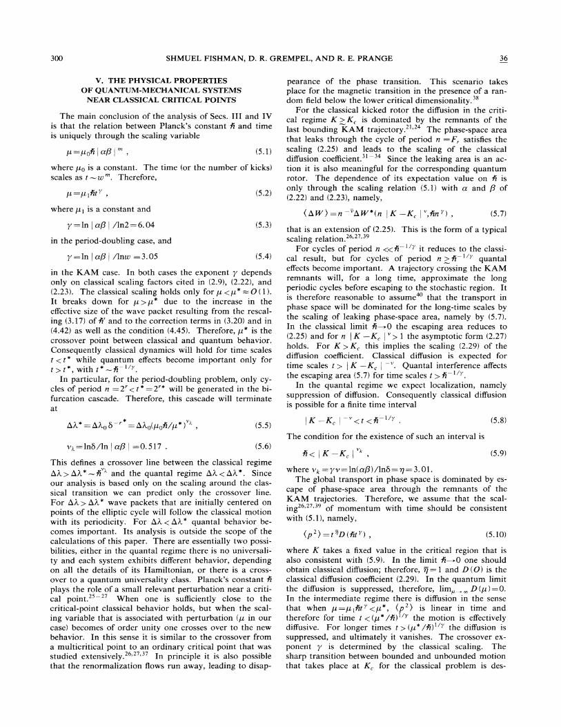
FIG. 1. The average of the momentum squared E(t) for wavepackets centered around Io ——0 (solid line) for K =1.5, wherePlanck's constant fi takes the values (a) ~; =0.001 20, (b)~; =0.003 38. The straight (dashed) line shows the behavior E(t)would exhibit if the diffusion would not be suppressed. The ar-row marks the crossover point at t*.

00+K cos8 g 6(t n)— (6.2)

Since the localization length increases with Klfi (for thenoncritical regime see Refs. 42 and 43), the main difficultyin the calculations that are presented in this section re-sults from the large basis that is required for the numeri-cal solution of (6.2). The solution was obtained in the an-gular momentum representation by the same method thatwas used in Ref. 12. The expansion coefficients of thewave function g immediately after a kick were calculatedand these enabled us to calculate the expectation valueE(t)= (p }. Some plots of E(t) that are representativefor K ~ K, are depicted in Figs. 1 and 2. After a short in-itial time with an irregular shape, there is a regime whereE(t) is linear in t, a behavior that is similar to classicaldiffusion. This regime terminates after the crossover timet* that is marked by an arrow in Figs. 1 and 2. Fort & t* the growth of E(t) with time is slower than thelinear diffusive growth. We interpret this as a result ofquantal localization. We found this behavior for severalvalues of K in the range 1.5 & K & 5.

We used the following two choices of the initialwavefunction: (a) An eigenstate of angular momentumlo =0, and (b) a wave packet with angular momentum l insome interval around a state lp and with a narrow max-

imum as a function of the angle around 0=0. The valueof lp was varied. These initial conditions correspond toclassical initial distributions where (a) the angle is distri-buted uniformly in the interval 0 & 0 & 2~, while themomentum vanishes, (b) the angle is distributed with highprobability near 0=0 while the momentum is nearpp = Ipk 0, namely the distribution is peaked near thehyperbolic Axed point 0=0, p =0. The rate of growth ofE(t) in the linear regime for the various initial wave func-tions is close to the classical diffusion coefficient for thecorresponding classical initial distributions. Note that theclassical diffusion coefficient depends on the initial condi-tions due to trapping in islets of stability. ' ' In someof the calculations we averaged the series E (t) over initialwave packets with various values of Ip. The resulting be-havior of E(t), for example the one presented in Fig. 2, isnot affected much by this averaging. For K &K, theshape of E(t) is very different from the one of Fig. 1.After a few steps it saturates at its maximal value and per-forms small oscillations around it. In particular there isno regime of linear increase of E(t). This is also the be-havior expected for the corresponding classical systemsince the motion is bounded by a KAM trajectory.

302 SHMUEL FISHMAN, D. R. GREMPEL, AND R. E. PRANQE

E (I)

30

20

50-(b)

250I

500 750

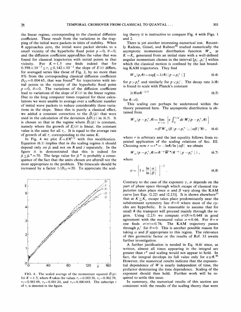
In Fig. 3 we plot lnt* versus~

1nfi ~. The continuousline corresponds to the result expected from the scalingtheory with @=3.05. We see that the results are con-sistent with the scaling theory but the deviations are large.

There is some arbitrariness in the determination of thepoint t* as is seen from Figs. 1 and 2: It is probably re-sponsible for the large scatter of the points of Fig. 3. Forthis reason we numerically determine the exponent y in adifferent way. If the scaling theory is correct (6.1) impliesthat E(t)/t is a function of p only at least for p &p*.Therefore, the values it takes as a function of p should beidentical for various values of ~;. This should hold exact-ly in the asymptotic limit %~K„~;~0but it should besatisfied approximately in the vicinity of this limit. There-fore we calculated numerically the deviation

N

~(y)= —g f dp[1 —D, (p)/(D(p))], (6.3)Pl

where D(p) are the values of E(t)/t found numericallyfor R=r;, while (D(P) ) =(1/1V)g+ i D, (p) is their aver-age. The exponent y that is evaluated in this way is theone that minimizes bD(y). The domain of integration ischosen so that p& &p ' &pz. The numerically evaluatedexponent y varies slightly when the range (p, &,p2) isvaried. We verified that for E =1.5, 1.65, 1.75, and 2.0the exponent y is in the range 2. 5 & y & 3.5. For K = 1.5and 1.65 the most probable value is approximately @=3.The range of variation of A' over which (6.1) is found to besatisfied is the largest for K =1.5. As a test we repeatedour analysis for K =5, that is far outside the critical re-gime. As expected it was concluded that (6.1) probablydoes not hold. Our data definitely rule out the possibilityy&2. 3 even if(6.1) holds for K=5. For p, ~p* thescal-ing relation (6.1) with y' of (5.4) breaks down and theanalysis of this regime is out of the scope of the presentpaper. In the calculations of this section we used onlyfew initial wave packets for each value of JC and R, conse-quently there are strong variations (of the order of 15%%uo

for K =1.5) in the value of the rate of growth of E(t) in

E (tI

30

10

250 500 750

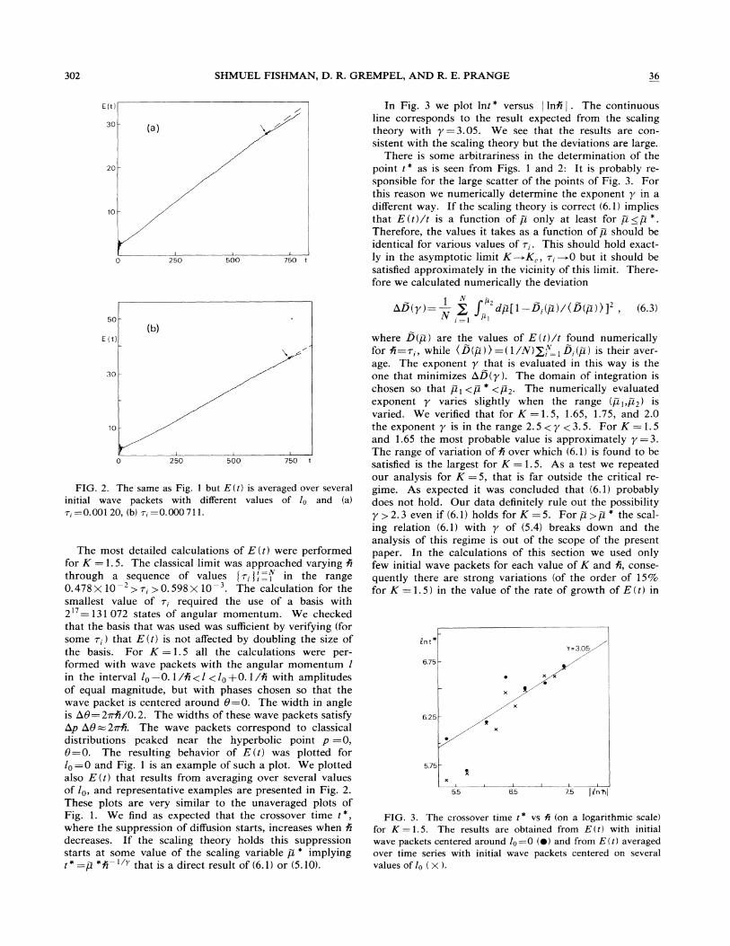
FIG. 2. The same as Fig. 1 but E(t) is averaged over severalinitial wave packets with different values of lo and (a)

~; =0.001 20, (b) ~; =0.000711.

The most detailed calculations of E(t) were performedfor K = 1.5. The classical limit was approached varying A

through a sequence of values Ir, I,':, in the range0.478&10 ~~; &0.598&10 . The calculation for thesmallest value of ~; required the use of a basis with2' =131072 states of angular momentum. We checkedthat the basis that was used was sufficient by verifying (forsome r;) that E(t) is not affected by doubling the size ofthe basis. For K = 1.5 all the calculations were per-formed with wave packets with the angular momentum lin the interval lo —0. 1/A&l &lo+0. 1/A with amplitudesof equal magnitude, but with phases chosen so that thewave packet is centered around 0=0. The width in angleis 60=2mb/0. 2. The widths of these wave packets satisfyAp 60=2M. The wave packets correspond to classicaldistributions peaked near the hyperbolic point p =0,0=0. The resulting behavior of E(t) was plotted forlo ——0 and Fig. 1 is an example of such a plot. We plottedalso E(t) that results from averaging over several valuesof 10, and representative examples are presented in Fig. 2.These plots are very similar to the unaveraged plots ofFig. 1. We find as expected that the crossover time t',where the suppression of diffusion starts, increases when Rdecreases. If the scaling theory holds this suppressionstarts at some value of the scaling variable p * implyingt'=p*A' ''r that is a direct result of(6.1) or (5.10).

6.75—

v=305

6.25

5,75—

5.5 6.5I I

Ignis~

FICx. 3. The crossover time t* vs A (on a logarithmic scale)for K =1.5. The results are obtained from E(t) with initialwave packets centered around Io ——0 (~ ) and from E(t) averagedover time series with initial wave packets centered on severalvalues of Io (&& ).


the linear regime, corresponding to the classical diffusioncoefficient. These result from the variations in the trap-ping of the initial wave packets in islets of stability. WhenA approaches zero, the initial wave packet shrinks to asmall vicinity of the hyperbolic fixed point p =0, 0=0,and the diffusion coefficient approa'ches the value that wasfound for classical trajectories with initial points in thatvicinity. For K = 1.5 one finds indeed that for0.598&&10 &~; &0. 142)&10 the slope of E(t) differs,for averaged series like those of Fig. 2, by no more than8% from the corresponding classical diffusion coefficientDc& ——0.00465, that was found for trajectories with ini-tial points in the vicinity of the hyperbolic fixed pointp =0, I9=0. The variations of the diffusion coefficientlead to variations of the slope of E (t) in the linear regime.Due to the long computer times required for these calcu-lations we were unable to average over a sufficient numberof initial wave packets to reduce considerably these varia-tions in the slope. Since this is purely a classical effect,we added a constant correction to the D;(p) that wereused in the calculation of the deviation ~(y) in (6.3). Itis chosen so that in the regime where D, (p, ) is constant,namely where the growth of E;(t) is linear, the constantvalue is the same for all ~;. It is equal to the average rateof growth of all ~; corresponding to the same K.

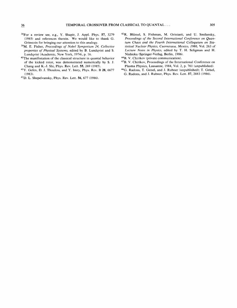
In Fig. 4 we plot E=EA' with this modification.Equation (6.1) implies that in the scaling regime it shoulddepend only on p, and not on A and t separately. In thefigure it is demonstrated that this is indeed forp(p*=70. The large value for p* is probably a conse-quence of the fact that the units chosen are afterall not themost appropriate to the problem. The timescale should beincreased by a factor 1/Dc] =20. To appreciate the scal-

ing theory it is instructive to compare Fig. 4 with Figs. 1

and 2.There is yet another interesting numerical test. Recent-

ly Radons, Geisel, and Rubner studied numerically theasymptotic momentum distribution function W atK =K, generated from an initial state with a well-definedangular momentum chosen in the interval [p, ,p+] withinwhich the classical motion is confined by the last bound-ing KAM trajectories. They find

W„(p,A')-exp[ —A, (A')~ p —p+

~ ] (6.4)

for p &p,* and similarly for p &p, . The decay rate A.(A')

is found to scale with Planck's constant

(6.&)

where r is arbitrary and the last equality follows from re-peated application of the scaling relations of Sec. III.Choosing now r =r*= —Inh'/In

~ap

~

we obtain

W„(p p+, fi)=A W— '(fi~p —p+

~),

where

(6.7)

—1

ln/a/ln [P

(6.8)

for A'~0.This scaling can perhaps be understood within the

theory presented here. The asymptotic distribution is ob-tained from

W„(p —p+, A')= lim e f dt W, (p —p+, fi)e~ oo 0

=P"W „(P i p —p,' ~, ~

o'P~

"&),

E-(.5)

J

1,'

4)

0 l

40 80I

120 160

FIG. 4. The scaled average of the momentum squared E(p, )

for K = 1.5, where fi takes the values ~& ——0.003 38, ~2 ——0.002 39,v3 —0.00 1 69, ~4 ——0.00 1 20, and ~&

——0.000 845. The subscript iof ~; is denoted in the figure.

Contrary to the case of the exponent y, 0. depends on thepart of phase space through which escape of classical tra-jectories takes place since a and p vary along the KAMcurve [see Eqs. (2.22) and (2.23)]. It is shown elsewherethat at K )K, escape takes place predominantly near thesubdominant symmetry line I9=0 where most of the cy-cles are hyperbolic. It is reasonable to assume that forsmall A the transport will proceed mainly through the re-gion. Using (2.23) we compute cr(O) =0.648 in goodagreement with the measured value o. =0.66. For 0=~one finds cr(~) =0.76. The KAM trajectory passesthrough p+ for 0=0. This is another possible reason fortaking a and P appropriate to this region. The relevanceof this geometric factor or the results of Ref. 33 awaitsfurther investigation.

A further justification is needed in Eq. (6.6) since, aswritten, almost all times appearing in the integral aregreater than t* and scaling would not appear to hold. Infact, the integral develops its full value only for @=A.However, the numerical results indicate that the exponen-tial dependence of W is nearly independent of time, theprefactor dominating the time dependence. Scaling of theexponent should then hold. Further work will be re-quired to settle this issue.

In summary, the numerical results of this section areconsistent with the results of the scaling theory that were

SHMUEL FISHMAN, D. R. GREMPEL, AND R. E. PRANGE 36

summarized in Sec. V. Note that the measured quantitiesin these cases are definitely quantum interference or tun-neling effects. This is obvious in the tunneling throughthe KAM trajectory at the critical value of IC. In the caseof diffusion for K~K„ it follows since the same break-down of scaling occurs for many initial wave packets,which have different classical behavior. We hope that ad-vances in computational power will enable us to producemore definitive evidence determining the correctness ofscaling theory in the future.

After the short version of this work was published (Ref.17) we were informed by Chirikov that he andShepelyansky obtained y =3 in the framework of an ap-proximate resonance theory for the disappearance of thelast bounding KAM trajectory. They performed numer-ical tests that were consistent with the analytical predic-tions. Their calculations, as well as ours, are not accurateenough to distinguish between y=3 and @=3.05. Theirinterpretation of y is different from ours, but the actualpredictions of the two approaches are equivalent.

ACKNOWLEDGMENTS

We enjoyed useful discussions and correspondence withmany of our colleagues, in particular with D. Bensimon,M. V. Berry, B. V. Chirikov, L. P. Kadanoff; G. Radons,and U. Smilansky. Wh thank M. Feingold, A. E. Stutz,and C. S. Wang for help with numerical processes. Thework was supported in part by the U.S.—Israel BinationalScience Foundation (BSF), by the Bat-Sheva de RotschildFund for Advancement of Science and Technology, andby the U.S. National Science Foundation through GrantNo. DMR-82-13768.

Some of the work was done at the Aspen Center forPhysics (Aspen, CO). One of us, S.F., thanks the Univer-sity of Maryland for the hospitality during several visitsthere. D.R.G. and S.F. thank the Einstein Summer Insti-tute for hospitality at the Weizmann Institute where thework was started. One of us, R.E.P., thanks the InstituteMax Laue —Paul Langevin for hospitality in the finalstages of work.

~M. V. Berry, in Chaotic Behavior of Deterministic Systems,Proceedings of Les Houches Summer School, Les Houches,1981, edited by G. Iooss, R. H. G. Helleman, and R. Stora(North-Holland, Amsterdam, 1983).

G. Zaslavsky, Phys. Rep. 80, 158 (1981).3P. Pechukas, Phys. Rev. Lett. 51, 943 (1983).4M. V. Berry, Ann. Phys. (N.Y.) 131, 163 (1981); M. V. Berry

and M. Tabor, Proc. R. Soc. London Ser. A 356, 375 (1977);M. V. Berry, ibid. 400, 229 (1985).

~O. Bohigas, M. J. Giannoni, and C. Schmit, Phys. Rev. Lett.52, 1 (1984).

M. Shapiro and G. Goelrnan, Phys. Rev. Lett. 53, 1714 (1984).7M. Feingold, N. Moiseyev, and A. Peres, Phys. Rev. A 30, 509

(1984).G. Casati, B. V. Chirikov, F. M. Israilev, and J. Ford, in Sto-

chastic Behavior in Quantum and Classical Hamiltonian Systems, Vol. 93 of Lecture Notes in Physics, edited by G. Casatiand J. Ford (Springer, Berlin, 1979).

B. V. Chirikov, F. M. Izrailev, and D. L. Shepelvanski, Sov.Sci. Rev. Sec. C2, 209 (1981).T. Hogg and B. A. Huberman, Phys. Rev. Lett. 48, 711 (1982);Phys. Rev. A 28, 22 (1983).

~ S. Fishman, D. R. Grempel, and R. E. Prange, Phys. Rev.Lett. 49, 509 (1982).D. R. Grempel, R. E. Prange, and S. Fishman, Phys. Rev. A29, 1639 (1984).

' R. E. Prange, D. R. Grempel, and S. Fishman, in Chaotic Be-havior in Quantum Systems, Proceedings of the Corno Confer-ence on Quantum Chaos, edited by G. Casati (Plenutn, NewYork, 1984).

'4H. J. Korsch and M. V. Berry, Physica 30, 627 (1981).~5M. V. Berry, N. L. Balazs, M. Tabor, and A. Voros, Ann.

Phys. (N.Y.) 122, 26 (1979).6R. Blumel and U. Smilanski, Phys. Rev. Lett. 52, 137 (1984);

G. Casati, B. V. Chirikov, and D. L. Shepelyansky, ibid. 53,2525 (1984); R. Jensen, ibid. 49, 1365 (1982).

' Some of the results are summarized in D. R. Grempel, S. Fish-man, and R. E. Prange, Phys. Rev. Lett. 53, 1212 (1984).

'8N. Moiseyev and A. Peres, J. Chem. Phys. 79, 5945 (1983).

' H. Frahm and H. J. Mikeska, Z. Phys. B 60, 117 (1985).J. M. Greene, R. S. McKay, F. Vivaldi, and M. J. Feigen-baum, Physica (Utrecht) 30, 468 (1981); P. Collet, J. P. Eck-mann, and H. Koch, ibid. 30, 457 (1981); T. C. Bountis, ibid.30, 577 (1981).

'R. S. MacKay, Ph. D. thesis, Princeton University (1982); R. S.MacKay, Physica 70, 283 (1983).B. V. Chirikov, Phys. Rep. 52, 263 (1979).J. M. Greene, J. Math. Phys. 20, 1183 (1981).L. P. Kadanoff, Phys. Rev. Lett. 47, 1641 (1981); S. J. Shenkerand L. P. Kadanoff, J. Stat. Phys. 27, 631 (1982); L. P. Ka-danoff, in Melting Localization and Chaos, edited by R. K.Kalia and P. Vashishta (North-Holland, New York, 1982).

2~K. G. Wilson and J. Kogut, Phys. Rep. 12C, 75 (1974).M. E. Fisher, Rev. Mod. Phys. 46, 597 (1974).

27S.-K. Ma, Modern Theory of Critical Phenomena (Benjamin,Reading, Mass. , 1976).M. E. Fisher, in Critical Phenomena, Proceedings of the Inter-national School of Physics "Enrico Fermi, " Course LI, Varen-na, 1972, edited by M. S. Green (Academic, New York, 1972).(a) J. Crutchfield, M. Nauenberg, and J. Rudnick, Phys. Rev.Lett. 46, 933 (1981); B. Shraiman, C. E. Wayne, and P. C.Martin, ibid. 46, 935 (1981); (b) M. J. Feigenbaum and B.Hasslacher, ibid. 49, 605 (1982).

3oL. S. Schulman, Techniques and Applications of Path Integration (Wiley, New York, 1981).D. Ben-Simon and L. P. Kadanoff, Physica 13D, 82 (1984).R. S. MacKay, J. D. Meiss, and I. C. Percival, Phys. Rev.Let t: 52, 697 (1984); Physica 13D, 55 (1984).

33I. Dana and S. Fishman, Physica 170, 63 (1985).4A. B. Rechester (private communication).

35R. Blumel, R. Meir, and U. Smilansky, Phys. Lett. 103A, 353(1984).

6M. Hillery, R. F. O' Connell, M. O. Scully, and E. P. Wigner,Phys. Rep. 106, 121 (1984); N. L. Balazs and B. K. Jennings,ibid. 104, 347 (1984).A. Aharony, in Phase Transitions and Critical Phenomena,edited by C. Domb and M. S. Green (Academic, New York,1976), Vol. 6, p. 357.


For a review see, e.g. , Y. Shapir, J. Appl. Phys. 57, 3279(1985) and references therein. We would like to thank G.Grinstein for bringing our attention to this analogy.

39M. E. Fisher, Proceedings of Nobel Symposium 24, Collectiveproperties of Physical Systems, edited by B. Lundqvist and S.Lundqvist (Academic, New York, 1974), p. 16.

~The manifestation of the classical structure in quantal behaviorof the kicked rotor, was demonstrated numerically by S. J.Chang and K.-J. Shi, Phys. Rev. Lett. 55, 269 (1985).

'Y. Gefen, D. J. Thouless, and Y. Imry, Phys. Rev. B 28, 6677(1983).

4~D. L. Shepelvansky, Phys. Rev. Lett. 56, 677 (1986).

R. Blumel, S. Fishman, M. Griniasti, and U. Smilansky,Proceedings of the Second International Conference on Quanturn Chaos and the Fourth International Co11oquium on Sta-tistica1 Nuclear Physics, Cuernevaca, Mexico, 1986, Vol. 263 ofLecture Notes in Physics, edited by T. H. Seligman and H.Nishioka (Springer-Verlag, Berlin, 1986).

~B. V. Chirikov (private communication).45B. V. Chirikov, Proceedings of the International Conference on

Plasma Physics, Lausanne, 1984, Vol. 2, p. 761 (unpublished).G. Radons, T. Geisel, and J. Rubner (unpublished); T. Geisel,G. Radons, and J. Rubner, Phys. Rev. Lett. 57, 2883 (1986).

temporal crossover from classical to quantal behavior near dynamical critical points

Documents