Technological Progress

Some Definitions

A capital saving technological progress (or invention) allows producers

to produce the same amount with relatively less capital input.

A labor saving technological progress (or invention) allows producers

to produce the same amount with relatively less labor input.

A neutral technological progress allows producers to produce more with

same capital labor ratio ( do not save relatively more of either input)

i) "Hicks neutral" : Ratio of marginal products remain the same for a

given capital labor ratio. Hicks neutrality implies the production function

can be written as:

Y = T (t)F (K,L)

ii) "Harrod neutral": relative input shares K.Fk/LFLremain the same

for a given capital output ratio

Harrod neutrality implies the production function can be written as:

Y = F [K,LT (t)] (labor-augmenting form)

where T (t) is the index of the technology and·T (t) > 0

labor-augmenting: it raises output in the same way as an increase in the

stock of labor.

iii) "Solow neutral": relative input shares LFL/K.Fkremain the same for

a given labor output ratio

Solow neutrality implies the production function can be written as:

Y = F [KT (t), L] (capital-augmenting form)

Solow Model with labor augmenting technological progress

Suppose the technology T (t) grows at rate x

·K(t) = I(t)− δK(t) = sF (K(t), T (t)L(t))− δK(t) (29)

Dividing by L(t)·k = sF (k, T (t))− (n + δ)k and

·kk = s

F (k,T (t))k − (n + δ)

The average product of per capita capital F (k,T (t))k now increases over

time because the T (t) grows at a rate x.

Steady state growth rate: By definition the steady state growth rateµ ·kk

¶∗is constant

sF (k∗,T (t))

k∗ − (n + δ) =constant

Since F is CRS, F (k,T (t))k = F (1,

T (t)k )This implies that T (t) and k grow

at the same rate x, because s,n and δ are constantsµ ·kk

¶∗= x

Moreover since y = F (k, T (t)) = kF (1,T (t)k )

à ·y

y

!∗= x (30)

and c = (1− s)y,³ ·cc

´=

µ(1−s) ·y(1−s)y

¶= x

Transitional Dynamics

Define: effective amount of labor=physical quantity of labor× efficiency

of labor = L× T (t) ≡∧L

∧k = K

LT (t)= k

T (t)= capital per unit of effective labor.

∧y = Y

LT (t)= F (

∧k, 1) = f(

∧k) = output per unit effective labor

We can rewrite·K = sF (K,T (t)L)− δK divide both sides by T (t)L

·K

T (t)L= sf(

∧k)− δ

∧k (31)

·∧k =

·³K

T (t)L

´=

LT (t)·K−K(

·LT (t)+L

·T (t))

T (t)2L2=

·K

T (t)L−

∧kn

T (t)L−

∧kx

T (t)L

Therefore·K

T (t)L=

·∧k +

∧kn

T (t)L+

∧kx

T (t)L

substituting in (31)

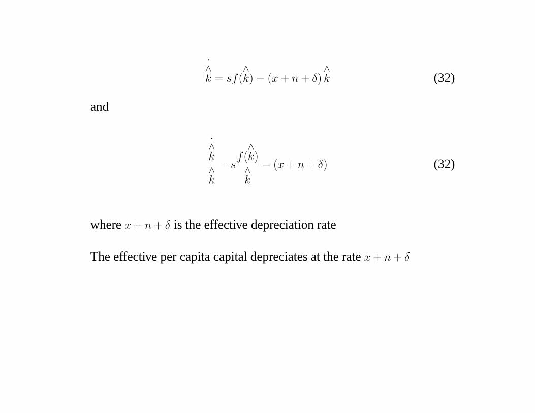
·∧k = sf(

∧k)− (x + n + δ)

∧k (32)

and

·∧k∧k

= sf(∧k)∧k

− (x+ n + δ) (32)

where x + n + δ is the effective depreciation rate

The effective per capita capital depreciates at the rate x + n + δ

Macro Lecture Notes– Ozan Hatipoglu

)( tkγ

tk

)( n+− δ

*k

Behavior of the growth rate in the Solow Model with labor augmenting technological progress (1)

Macro Lecture Notes– Ozan Hatipoglu

)( tk∧

γ

tk∧

)( xn ++δ

*∧

k

Behavior of the growth rate in the Solow Model with labor augmenting technological progress  (2)

∧

∧

t

t

k

kfs )(

Speed of Convergence:

The speed of convergence is given by

β = −∂(

·∧k∧k)

∂ log∧k

(33)

For the CD production fucntion·∧k∧k= sA(

∧k)−(1−α) − (x + n + δ)

or·∧k∧k= sAe−(1−α) log(

∧k) − (x+ n + δ)

β = (1− α)sA(∧k)−(1−α) (declines monotonically)

Near the steady state

sA(∧k)−(1−α) = (x+ n + δ)

β∗ = (1− α)(x+ n + δ) (34)

What does the data say about convergence?

Consider the benchmark case with

x = 0.02, n = 0.01 and δ = 0.05 (for US)

where x is the long term growth rate of GDP/ per capita

β∗ = (1− α)(x+ n + δ) = (1− α)(0.08) depends on α

Suppose α = 1/3(, based on data) then β∗ = 5.6% (half life of 12.5 years)

But the data says that β∗ ' 2 − 3% which implies α = 3/4 (too high for

physical capital)

-A broader definition of capital is needed to reconcile theory with the

facts

Extended Solow Model with human capital

Y = AKαHη [T (t)L]1−α−η and∧y = A

∧kα∧hη

(35)

·∧k +

·∧h = sA

∧kα∧hη

− (x + n + δ)

µ∧k +

∧h

¶(36)

It must be the case that returns to each type of capital are equal.

α∧y∧k− δ = η

∧y∧h− δ and

∧h = η

α

∧k

Using in (36)·∧k = s

∼A∧kα+η

− (δ + n + x) where∼A =constant

β∗ = (1− α− η)(x+ n + δ)

Now with α = 1/3(, based on data) then β∗ = 2.1% ( a better match)

What’s Wrong with Neoclassical Theory??

-Does not explain long-term consistent per capita growth rates .

-Can not maintain pefect competition assumption when technological

progress is not exogenous.

The AK Model

Y = AK·kk = sA− (n + δ) > 0 for all k if sA > (n + δ)

does not exhibit conditional convergence.. How?

How about

Y = AK +BKαL1−α whereA > 0, B > 0 and 0 < α < 1

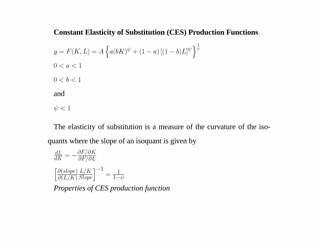
Constant Elasticity of Substitution (CES) Production Functions

y = F (K,L) = Ana(bK)ψ + (1− a) [(1− b)L]ψ

o 1ψ

0 < a < 1

0 < b < 1

and

ψ < 1

The elasticity of substitution is a measure of the curvature of the iso-

quants where the slope of an isoquant is given bydLdK = −∂F/∂K

∂F/∂Lh∂(slope)∂(L/K)

L/KSlope

i−1= 11−ψ

Properties of CES production function

1) The elasticity of substitution between capital and labor, 11−ψ ,is con-

stant

2)CRS for all values of ψ

3) As ψ →−∞, the production function approaches Y = min [bK, (1− b)L] ,

As ψ → 0, Y = (constant)KaL1−a (CD)

For ψ = 1, Y = abK +(1− a)(1− b)L (linear) so that K and L are perfect

substitutes (infinite elasticity of substitution)

Proof: Take log of Y and apply L’Hospital’s rule. i.e.find limψ→0 [log Y ]

Transitional Dynamics with CES production function·kk = s

f(k)k − (n + δ)

Note that for CES

f 0(k) = Aabψhabψ + (1− a)(1− b)ψk−ψ

i1−ψψ

andf(k)k = A

habψ + (1− a) (1− b)ψ k−ψ

i 1ψ

i) 0 < ψ < 1

limk→∞£f 0(k)

¤= limk→∞

hf(k)k

i= Aba

1

ψ > 0

limk→0£f 0(k)

¤= limk→0

hf(k)k

i=∞

Therefore, CES can exhibit can generate endogenous growth for 0 <

ψ < 1, if savings rates are high enough.

Macro Lecture Notes– Ozan Hatipoglu

tk

)( n+δ

CES Model with and

ψ1

sAbakkfs )(

)10( <<ψ nsAba +>δψ1

0>kγ

ii) ψ < 0

limk→∞£f 0(k)

¤= limk→∞

hf(k)k

i= 0

limk→0£f 0(k)

¤= limk→0

hf(k)k

i= Aba

1

ψ <∞

No endogenous growth, negative growth rates are possible for low val-

ues of sMacro Lecture Notes– Ozan Hatipoglu

tk

)( n+δ

CES Model with and

ψ1

sAba

kkfs )(

)0( <ψ nsAba +< δψ1

0<kγ

Poverty TrapsMacro Lecture Notes– Ozan Hatipoglu

tk

1+tk

*k

Poverty Traps  in the Solow Model

)( tkG

tt kk =+1

*trapk

for some range of k, the average product of capital is increasing in k

- non-constant savings rates

- increasing returns with learning by doing and spillovers

Asimple model

Suppose the country has access to two technologies

yA = Akα

yB = Bkα − b

where B>A. To employ yB gov’t has to incur a setup cost of b per worker.

Under what conditions will the government incur b?

yA ≤ yB

or Akα ≤ Bkα − b

and k ≥∼k where

∼k =

hb

B−Ai 1α

·kk = sAk

α

k − (n + δ)·kk = sBk

α−bk − (n + δ)