techniques for tracking, evaluating, and reporting the
TRANSCRIPT

United States Office Of Water EPA 841-B-00-007Environmental Protection (4503F) January 2001Agency
TECHNIQUES FOR TRACKING,EVALUATING, AND REPORTINGTHE IMPLEMENTATION OFNONPOINT SOURCE CONTROLMEASURES
URBAN

TECHNIQUES FOR TRACKING, EVALUATING,AND REPORTING THE IMPLEMENTATION
OF NONPOINT SOURCE CONTROLMEASURES
III. URBAN
FinalJanuary 2001
Prepared for
Nonpoint Source Pollution Control BranchOffice of Water
United States Environmental Protection AgencyWashington, DC
Prepared under
EPA Contract No. 68-C-99-249Work Assignment No. 0-25

i
CONTENTS
Chapter 1 Introduction1.1 Purpose of Guidance . . . . . . . . . . . . . . . . . . . . . . . . . . . . . . . . . . . . . . . . . . . . . . . . . . . 1-11.2 Background . . . . . . . . . . . . . . . . . . . . . . . . . . . . . . . . . . . . . . . . . . . . . . . . . . . . . . . . . . 1-21.3 Types of Monitoring . . . . . . . . . . . . . . . . . . . . . . . . . . . . . . . . . . . . . . . . . . . . . . . . . . . 1-31.4 Quality Assurance and Quality Control . . . . . . . . . . . . . . . . . . . . . . . . . . . . . . . . . . . . . 1-51.5 Data Management . . . . . . . . . . . . . . . . . . . . . . . . . . . . . . . . . . . . . . . . . . . . . . . . . . . . . 1-5
Chapter 2 Methods to Inventory BMP Implementation2.1 Regulated Activities . . . . . . . . . . . . . . . . . . . . . . . . . . . . . . . . . . . . . . . . . . . . . . . . . . . . 2-1
2.1.1 Erosion and Sediment Control . . . . . . . . . . . . . . . . . . . . . . . . . . . . . . . . . . . . . . 2-12.1.2 Septic Systems . . . . . . . . . . . . . . . . . . . . . . . . . . . . . . . . . . . . . . . . . . . . . . . . . . 2-32.1.3 Runoff Control and Treatment . . . . . . . . . . . . . . . . . . . . . . . . . . . . . . . . . . . . . . 2-6
2.2 Tracking BMP Operation and Maintenance . . . . . . . . . . . . . . . . . . . . . . . . . . . . . . . . . 2-62.3 Geographic Information Systems and BMP Implementation/Effectiveness . . . . . . . . . 2-82.4 Summary of Program Elements for a Successful BMP Inventory . . . . . . . . . . . . . . . . 2-10
Chapter 3 Sampling Design3.1 Introduction . . . . . . . . . . . . . . . . . . . . . . . . . . . . . . . . . . . . . . . . . . . . . . . . . . . . . . . . . . 3-1
3.1.1 Study Objectives . . . . . . . . . . . . . . . . . . . . . . . . . . . . . . . . . . . . . . . . . . . . . . . . 3-13.1.2 Probabilistic Sampling . . . . . . . . . . . . . . . . . . . . . . . . . . . . . . . . . . . . . . . . . . . . 3-23.1.3 Measurement and Sampling Errors . . . . . . . . . . . . . . . . . . . . . . . . . . . . . . . . . 3-103.1.4 Estimation and Hypothesis Testing . . . . . . . . . . . . . . . . . . . . . . . . . . . . . . . . . 3-12
3.2 Sampling Considerations . . . . . . . . . . . . . . . . . . . . . . . . . . . . . . . . . . . . . . . . . . . . . . . 3-133.2.1 Urbanized and Urbanizing Areas . . . . . . . . . . . . . . . . . . . . . . . . . . . . . . . . . . . 3-143.2.2 Available Resources and Tax Base . . . . . . . . . . . . . . . . . . . . . . . . . . . . . . . . . 3-143.2.3 Proximity to Sensitive Habitats . . . . . . . . . . . . . . . . . . . . . . . . . . . . . . . . . . . . 3-143.2.4 Federal Requirements . . . . . . . . . . . . . . . . . . . . . . . . . . . . . . . . . . . . . . . . . . . 3-143.2.5 Sources of Information . . . . . . . . . . . . . . . . . . . . . . . . . . . . . . . . . . . . . . . . . . . 3-15
3.3 Sample Size Calculations . . . . . . . . . . . . . . . . . . . . . . . . . . . . . . . . . . . . . . . . . . . . . . . 3-163.3.1 Simple Random Sampling . . . . . . . . . . . . . . . . . . . . . . . . . . . . . . . . . . . . . . . . 3-183.3.2 Stratified Random Sampling . . . . . . . . . . . . . . . . . . . . . . . . . . . . . . . . . . . . . . 3-233.3.3 Cluster Sampling . . . . . . . . . . . . . . . . . . . . . . . . . . . . . . . . . . . . . . . . . . . . . . . 3-263.3.4 Systematic Sampling . . . . . . . . . . . . . . . . . . . . . . . . . . . . . . . . . . . . . . . . . . . . 3-263.3.5 Concluding Remarks . . . . . . . . . . . . . . . . . . . . . . . . . . . . . . . . . . . . . . . . . . . . 3-27
Chapter 4 Methods for Evaluating Data4.1 Introduction . . . . . . . . . . . . . . . . . . . . . . . . . . . . . . . . . . . . . . . . . . . . . . . . . . . . . . . . . . 4-14.2 Comparing the Means from Two Independent Random Samples . . . . . . . . . . . . . . . . . 4-24.3 Comparing the Proportions from Two Independent Samples . . . . . . . . . . . . . . . . . . . . 4-34.4 Comparing More Than Two Independent Random Samples . . . . . . . . . . . . . . . . . . . . . 4-44.5 Comparing Categorical Data . . . . . . . . . . . . . . . . . . . . . . . . . . . . . . . . . . . . . . . . . . . . . 4-4

Contents
ii
Chapter 5 Conducting the Evaluation5.1 Introduction . . . . . . . . . . . . . . . . . . . . . . . . . . . . . . . . . . . . . . . . . . . . . . . . . . . . . . . . . . 5-15.2 Choice of Variables . . . . . . . . . . . . . . . . . . . . . . . . . . . . . . . . . . . . . . . . . . . . . . . . . . . . 5-35.3 Expert Evaluations . . . . . . . . . . . . . . . . . . . . . . . . . . . . . . . . . . . . . . . . . . . . . . . . . . . . . 5-6
5.3.1 Site Evaluations . . . . . . . . . . . . . . . . . . . . . . . . . . . . . . . . . . . . . . . . . . . . . . . . . 5-65.3.2 Rating Implementation of Management Measures and Best
Management Practices . . . . . . . . . . . . . . . . . . . . . . . . . . . . . . . . . . . . . . . . . . . 5-115.3.3 Rating Terms . . . . . . . . . . . . . . . . . . . . . . . . . . . . . . . . . . . . . . . . . . . . . . . . . . 5-145.3.4 Consistency Issues . . . . . . . . . . . . . . . . . . . . . . . . . . . . . . . . . . . . . . . . . . . . . . 5-155.3.5 Postevaluation Onsite Activities . . . . . . . . . . . . . . . . . . . . . . . . . . . . . . . . . . . 5-16
5.4 Self-Evaluations . . . . . . . . . . . . . . . . . . . . . . . . . . . . . . . . . . . . . . . . . . . . . . . . . . . . . . 5-175.4.1 Methods . . . . . . . . . . . . . . . . . . . . . . . . . . . . . . . . . . . . . . . . . . . . . . . . . . . . . . 5-175.4.2 Cost . . . . . . . . . . . . . . . . . . . . . . . . . . . . . . . . . . . . . . . . . . . . . . . . . . . . . . . . . 5-185.4.3 Questionnaire Design . . . . . . . . . . . . . . . . . . . . . . . . . . . . . . . . . . . . . . . . . . . . 5-21
5.5 Aerial Reconnaissance and Photography . . . . . . . . . . . . . . . . . . . . . . . . . . . . . . . . . . . 5-23
Chapter 6 Presentation of Evaluation Results6.1 Introduction . . . . . . . . . . . . . . . . . . . . . . . . . . . . . . . . . . . . . . . . . . . . . . . . . . . . . . . . . . 6-16.2 Audience Identification . . . . . . . . . . . . . . . . . . . . . . . . . . . . . . . . . . . . . . . . . . . . . . . . . 6-26.3 Presentation Format . . . . . . . . . . . . . . . . . . . . . . . . . . . . . . . . . . . . . . . . . . . . . . . . . . . . 6-2
6.3.1 Written Presentations . . . . . . . . . . . . . . . . . . . . . . . . . . . . . . . . . . . . . . . . . . . . . 6-46.3.2 Oral Presentations . . . . . . . . . . . . . . . . . . . . . . . . . . . . . . . . . . . . . . . . . . . . . . . 6-4
6.4 For Further Information . . . . . . . . . . . . . . . . . . . . . . . . . . . . . . . . . . . . . . . . . . . . . . . . . 6-6
References . . . . . . . . . . . . . . . . . . . . . . . . . . . . . . . . . . . . . . . . . . . . . . . . . . . . . . . . . . . . . . . . . R-1
Glossary . . . . . . . . . . . . . . . . . . . . . . . . . . . . . . . . . . . . . . . . . . . . . . . . . . . . . . . . . . . . . . . . . . G-1
Index . . . . . . . . . . . . . . . . . . . . . . . . . . . . . . . . . . . . . . . . . . . . . . . . . . . . . . . . . . . . . . . . . . . . . I-1
Appendix A: Statistical Tables . . . . . . . . . . . . . . . . . . . . . . . . . . . . . . . . . . . . . . . . . . . . . . . . A-1

Contents
iii
List of TablesTable 3-1 Example applications of four sampling designs for implementation
monitoring . . . . . . . . . . . . . . . . . . . . . . . . . . . . . . . . . . . . . . . . . . . . . . . . . . . . . 3-3Table 3-2 Errors in hypothesis testing . . . . . . . . . . . . . . . . . . . . . . . . . . . . . . . . . . . . . . . 3-13Table 3-3 Definitions used in sample size calculation equations . . . . . . . . . . . . . . . . . . . 3-17Table 3-4 Comparison of sample size as a function of various parameters . . . . . . . . . . . 3-20Table 3-5 Common values of (�
� + �2�)
2 for estimating sample size . . . . . . . . . . . . . . . 3-22Table 3-6 Allocation of samples . . . . . . . . . . . . . . . . . . . . . . . . . . . . . . . . . . . . . . . . . . . 3-25Table 3-7 Number of residences at each site implementing recommended
lawn care practices . . . . . . . . . . . . . . . . . . . . . . . . . . . . . . . . . . . . . . . . . . . . . . 3-27Table 4-1 Contingency table of observed resident type and
implemented BMP . . . . . . . . . . . . . . . . . . . . . . . . . . . . . . . . . . . . . . . . . . . . . . . 4-5Table 4-2 Contingency table of expected resident type and implemented BMP . . . . . . . . 4-5Table 4-3 Contingency table of implemented BMP and rating of
installation and maintenance . . . . . . . . . . . . . . . . . . . . . . . . . . . . . . . . . . . . . . . 4-6Table 4-4 Contingency table of implemented BMP and sample year . . . . . . . . . . . . . . . . 4-7Table 5-1 General types of information obtainable with self-evaluations
and expert evaluations . . . . . . . . . . . . . . . . . . . . . . . . . . . . . . . . . . . . . . . . . . . . 5-4Table 5-2 Example variables for management measure implementation analysis . . . . . . . 5-7
List of FiguresFigure 3-1 Simple random sampling from a list and a map . . . . . . . . . . . . . . . . . . . . . . . . 3-5Figure 3-2 Stratified random sampling from a list and a map . . . . . . . . . . . . . . . . . . . . . . . 3-7Figure 3-3 Cluster sampling from a list and a map . . . . . . . . . . . . . . . . . . . . . . . . . . . . . . . 3-8Figure 3-4 Systematic sampling from a list and a map . . . . . . . . . . . . . . . . . . . . . . . . . . . . 3-9Figure 3-5 Graphical presentation of the relationship between bias,
precision, and accuracy . . . . . . . . . . . . . . . . . . . . . . . . . . . . . . . . . . . . . . . . . 3-11Figure 5-1 Potential variables and examples of implementation
standards and specifications . . . . . . . . . . . . . . . . . . . . . . . . . . . . . . . . . . . . . . 5-5Figure 5-2 Sample draft survey for residential “good housekeeping” practice
implementation . . . . . . . . . . . . . . . . . . . . . . . . . . . . . . . . . . . . . . . . . . . . . . . 5-19Figure 6-1 Example of presentation of information in a written slide . . . . . . . . . . . . . . . . 6-3Figure 6-2 Example written presentation slide . . . . . . . . . . . . . . . . . . . . . . . . . . . . . . . . . . 6-4Figure 6-3 Example representation of data in the form of a pie chart . . . . . . . . . . . . . . . . . 6-4Figure 6-4 Graphical representation of data from construction site surveys . . . . . . . . . . . . 6-5

���
This guidance focuses on the methods thatcan be used to inventory specific types ofurban BMPs and the design of monitoringprograms to assess implementation of urbanmanagement measures and BMPs, withparticular emphasis on statisticalconsiderations.
CHAPTER 1. INTRODUCTION
1.1 PURPOSE OF GUIDANCE
This guidance is intended to assist federal,state, regional, and local environmentalprofessionals in tracking the implementation ofbest management practices (BMPs) used tocontrol urban nonpoint source pollution. Information is provided on methods forinventorying BMPs, the design and executionof sampling programs, and the evaluation andpresentation of results. The more regulatedand stable nature of urban areas presentopportunities for inventorying all BMPs versusthe statistical sampling required to assess BMPimplementation for agriculture or forestry. Inventorying BMP implementation requiresestablishing a program that tracks theimplementation or operation and maintenanceof all BMPs of certain types (e.g., septic tanksand erosion and sediment control practices). The guidance can help state and localgovernments by providing a subset of controls,both structural and nonstructural, that can besampled for:
• inspection programs,• maintenance oversight, and• implementation confirmation.
The focus of chapters 3 and 4 is on thestatistical approaches needed to properlycollect and analyze data that are accurate anddefensible. A properly designed BMPimplementation monitoring program can saveboth time and money. For example, the cost todetermine the degree to which pollutionprevention activities are conducted by an entireurban population would easily exceed mostbudgets, and thus statistical sampling of asubset of the population is needed. Guidanceis provided on sampling representative BMPs
to yield summary statistics at a fraction of thecost of a comprehensive inventory.
While it is not the focus of this guidance, somenonpoint source projects and programscombine BMP implementation monitoringwith water quality monitoring to evaluate theeffectiveness of BMPs in protecting waterquality on a watershed scale (Meals, 1988;Rashin et al., 1994; USEPA, 1993b). For thistype of monitoring to be successful, the scaleof the project should be small (e.g., awatershed of a few hundred to a few thousandacres). Accurate records of all the sources ofpollutants of concern, how these sources arechanging (e.g., new development), and aninventory of how all BMPs are operating arevital for this type of monitoring. Otherwise, itis impossible to accurately correlate BMPimplementation with changes in stream waterquality. This guidance does not addressmonitoring the implementation andeffectiveness of individual BMPs. It doesprovide information to help program managersgather statistically valid information to assessimplementation of BMPs on a more general(e.g., statewide) basis. The benefits ofimplementation monitoring are presented inSection 1.3.

Introduction Chapter 1
���
1.2 BACKGROUND
Because of the past and current successes incontrolling point sources, pollution fromnonpoint sources—sediment deposition,erosion, contaminated runoff, hydrologicmodifications that degrade water quality, andother diffuse sources of water pollution—isnow the largest cause of water qualityimpairment in the United States (USEPA,1995). Recognizing the importance ofnonpoint sources, Congress passed the CoastalZone Act Reauthorization Amendments of1990 (CZARA) to help address nonpointsource pollution in coastal waters. CZARAprovides that each state with an approvedcoastal zone management program developand submit to the U.S. EnvironmentalProtection Agency (EPA) and NationalOceanic and Atmospheric Administration(NOAA) a Coastal Nonpoint Pollution ControlProgram (CNPCP). State programs must“provide for the implementation” ofmanagement measures in conformity with theEPA Guidance Specifying ManagementMeasures For Sources Of Nonpoint PollutionIn Coastal Waters, developed pursuant toSection 6217(g) of CZARA (USEPA, 1993a). Management measures (MMs), as defined inCZARA, are economically achievablemeasures to control the addition of pollutantsto coastal waters, which reflect the greatestdegree of pollutant reduction achievablethrough the best available nonpoint pollutioncontrol practices, technologies, processes,siting criteria, operating methods, or otheralternatives (all of which are often referred toas BMPs). Many of EPA’s MMs arecombinations of BMPs. For example,depending on site characteristics,implementation of the Construction SiteErosion and Sediment Control MM might use
the following BMPs: brush barriers, filterstrips, silt fencing, vegetated channels, andinlet protection.
CZARA does not specifically require thatstates monitor the implementation of MMs andBMPs as part of their CNPCPs. StateCNPCPs must however, provide for technicalassistance to local governments and the publicfor implementing the MMs and BMPs. Section 6217(b) states:
Each State program . . . shall provide forthe implementation, at a minimum, ofmanagement measures . . . and shall alsocontain . . . (4) The provision of technicaland other assistance to local governmentsand the public for implementing themeasures . . . which may include assistance. . . to predict and assess the effectivenessof such measures . . . .
EPA and NOAA also have some responsibilityunder Section 6217 for providing technicalassistance to implement state CNPCPs. Section 6217(d), Technical assistance, states:
[NOAA and EPA] shall provide technicalassistance . . . in developing andimplementing programs. Such assistanceshall include: . . . (4) methods to predictand assess the effects of coastal land usemanagement measures on coastal waterquality and designated uses.
This guidance document was developed toprovide the technical assistance described inCZARA Sections 6217(b)(4) and 6217(d), butthe techniques can be used for similarprograms and projects. For instance,monitoring projects funded under Clean WaterAct (CWA) Section 319(h) grants, efforts to

IntroductionChapter 1
���
implement total maximum daily loadsdeveloped under CWA Section 303(d),stormwater permitting programs, and otherprograms could all benefit from knowledge ofBMP implementation.
Methods to assess the implementation of MMsand BMPs, then, are a key focus of thetechnical assistance to be provided by EPAand NOAA. Implementation assessments canbe done on several scales. Site-specificassessments can be used to assess individualBMPs or MMs, and watershed assessmentscan be used to look at the cumulative effects ofimplementing multiple MMs. With regard to“site-specific” assessments, individual BMPsmust be assessed at the appropriate scale forthe BMP of interest. For example, to assessthe implementation of MMs and BMPs forerosion and sediment control (E&SC) at aconstruction site, only the structures, areas,and practices implemented specifically forE&SC (eg., protection of natural vegetation,sediment basins, or soil stabilization practices)would need to be inspected. In this instancethe area physically disturbed by constructionactivities and the upslope area would be theappropriate site and scale.
However, if a state without a centralizedE&SC program were assessing erosion andE&SC in an area (e.g., coastal) of concern, itmight assess municipal E&SC programs. Inthis instance the “site” would be each urbanarea and implementation of municipalregulations, inspection and enforcementprograms, etc. would be checked. For bridgerunoff management, the scale might be bridgesover waterways that carry and average dailytraffic of 500 or more vehicles and the siteswould be individual bridges that meet thisrequirement. Site-specific measurements can
then be used to extrapolate to a program,watershed, or statewide assessment. There areinstances where a complete inventory of MMand BMP implementation across an entirewatershed or geographic area is preferred.
1.3 TYPES OF MONITORING
The term monitor is defined as “to check orevaluate something on a constant or regularbasis” (Academic Press, 1992). It is possibleto distinguish among various types ofmonitoring. Two types, implementation at aspecific time (i.e., a snapshot) and trend (i.e.,trends in implementation) monitoring, are thefocus of this guidance. These types ofmonitoring can be used to address thefollowing goals:
• Determine the extent to which MMs andBMPs are implemented in accordance withrelevant standards and specifications.
• Determine whether there has been a changein the extent to which MMs and BMPs arebeing implemented.
In general, implementation monitoring is usedto determine whether goals, objectives,standards, and management practices are beingimplemented as detailed in implementationplans. In the context of BMPs within stateCNPCPs, implementation monitoring is usedto determine the degree to which MMs andBMPs required or recommended by theCNPCPs are being implemented. If CNPCPscall for voluntary implementation of MMs andBMPs, implementation monitoring can be usedto determine the success of the voluntaryprogram (1) within a given monitoring period(e.g., 1 or 2 years); (2) during severalmonitoring periods, to determine any temporal

Introduction Chapter 1
���
trends in BMP implementation; or (3) invarious regions of the state.
Trend monitoring involves long-termmonitoring of changes in one or moreparameters. As discussed in this guidance,public attitudes, land use, and the use ofvarious urban BMPs are examples ofparameters that could be measured with trendmonitoring. Isolating the impacts of MMs andBMPs on water quality requires trendmonitoring.
Because trend monitoring involves measuringa change (or lack thereof) in some parameterover time, it is necessarily of longer durationand requires that a baseline, or starting point,be established. Any changes in the measuredparameter are then detected in reference to thebaseline.
Implementation and the related trendmonitoring can be used to determine (1) which MMs and BMPs are beingimplemented, (2) whether MMs and BMPs arebeing implemented as designed, and (3) the need for increased efforts to promote orinduce use of MMs and BMPs. Data fromimplementation monitoring, used incombination with other types of data, can beuseful in meeting a variety of other objectives,including the following (Hook et al., 1991;IDDHW, 1993; Schultz, 1992):
• To evaluate BMP effectiveness forprotecting natural resources.
• To identify areas in need of furtherinvestigation.
• To establish a reference point of overallcompliance with BMPs.
• To determine whether landowners areaware of BMPs.
• To determine whether landowners areusing the advice of urban BMP experts.
• To identify any BMP implementationproblems specific to a land ownership oruse category.
• To evaluate whether any urban BMPscause environmental damage.
• To compare the effectiveness of alternativeBMPs.
MacDonald et al. (1991) describes additionaltypes of monitoring, including effectiveness,baseline, project, validation, and compliancemonitoring. As emphasized by MacDonaldand others, these monitoring types are notmutually exclusive and the distinctions amongthem are usually determined by their purpose.
Effectiveness monitoring is used to determinewhether MMs or BMPs, as designed andimplemented, are meeting management goalsand objectives. Effectiveness monitoring is alogical follow-up to implementationmonitoring, because it is essential thateffectiveness monitoring include anassessment of the adequacy of the design andinstallation of MMs and BMPs. For example,the objective of effectiveness monitoring couldbe to evaluate the effectiveness of MMs andBMPs as designed and installed, or to evaluatethe effectiveness of MMs and BMPs that aredesigned and installed adequately or tostandards and specifications. Effectivenessmonitoring is not addressed in this guide, butis the subject of another EPA guidancedocument, Monitoring Guidance for

IntroductionChapter 1
���
Determining the Effectiveness of NonpointSource Controls (USEPA, 1997).
1.4 QUALITY ASSURANCE AND QUALITYCONTROL
An integral part of the design phase of anynonpoint source pollution monitoring projectis quality assurance and quality control(QA/QC). Development of a quality assuranceproject plan (QAPP) is the first step ofincorporating QA/QC into a monitoringproject. The QAPP is a critical document forthe data collection effort inasmuch as itintegrates the technical and quality aspects ofthe planning, implementation, and assessmentphases of the project. The QAPP documentshow QA/QC elements will be implemented. Itcontains statements about the expectations andrequirements of those for whom the data isbeing collected (i.e., the decision maker) andprovides details on project-specific datacollection and data management proceduresdesigned to ensure that these requirements aremet. Development and implementation of aQA/QC program, including preparation of aQAPP, can require up to 10 to 20 percent ofproject resources (Cross-Smiecinski andStetzenback, 1994). A thorough discussion ofQA/QC is provided in Chapter 5 of EPA’s Monitoring Guidance for Determining theEffectiveness of Nonpoint Source Controls(USEPA, 1997).
1.5 DATA MANAGEMENT
Data management is a key component of asuccessful MM or BMP implementationmonitoring effort. The systemused—including the quality control and qualityassurance aspects of data handling, how andwhere data are stored, and who manages the
stored data—determines the reliability,longevity, and accessibility of the data.Provided that data collection was well plannedand executed, an organized and efficient datamanagement system will ensure that the data:
• Can be used with confidence by those whomust make decisions based upon it,
• Will be useful as a baseline for similar datacollection efforts in the future,
• Will not become obsolete quickly, and
• Will be available to a variety of users formyriad applications.
Serious consideration is often not given to adata management system prior to a collectioneffort, which is precisely why it is so importantto recognize the long-term value of a smallinvestment of time and money in proper datamanagement. Data management competeswith other priorities for money, staff, and time,and if the importance and long-term value ofdata management is recognized early, the morelikely it will be to receive sufficient funding. Overall, data management might account foronly a small portion of a project’s total budget,but the return is great, considering that datacan be rendered virtually useless if data are notmanaged adequately.
Two important aspects of data that should beconsidered when planning the initial collectionand management systems are data life cycleand accessibility. The cycle has 5 stages: (1) data are collected; (2) data are checked forquality; (3) data are entered into a database; (4)data are used, and (5) data eventually becomeobsolete. The expected usefulness and lifespan of the data should be considered during

Introduction Chapter 1
���
the initial stages of planning a data collectioneffort, when the money, staff, and timedevoted to data collection must be weighedagainst its usefulness and longevity. Data withlimited uses and likely to become obsoletesoon after collection are a poorer investmentdecision than data with multiple applicationsand long life spans.
Data accessibility is a critical factor indetermining its usefulness. Data attainshighest value if widely accessible, if accessrequires the least staff effort, and if used byothers conveniently. If date are stored whereobtainable (with little assistance), use andsharing are more likely. The format for datastorage determines how conveniently data canbe used. Electronic storage in widely availableand used data formats makes for convenience. Storage as only a paper copy buried in a report,where any analysis requires entry into anelectronic format or time-consumingmanipulation, makes data extremelyinconvenient and thus unlikely to be used.
The following should be considered for thedevelopment of a data management strategy:
• What level of quality control should thedata be subject to? Data to be used for avariety of purposes or for importantdecisions merit careful quality controlchecks.
• Where and how will the data be stored? The options for data storage range from aprinted final report on a bookshelf to anelectronic data base accessible togovernment agencies and the public. Determining where and how data will bestored requires careful consideration of thequestion: How accessible should the databe?
• Who will maintain the data base? Datastored in a large data base might bemanaged by a professional manager, whiledata kept in agency files might be managedby people of various backgrounds overtime.
• How much will data management cost? As with all other aspects of data collection,data management costs money and must bebalanced with all other project costs.

���
CHAPTER 2. METHODS TO INVENTORY BMP IMPLEMENTATION
Because the potential for serious water qualitydegradation is high in urban areas, it isimportant to have a means to track theimplementation of BMPs used to control urbannonpoint source pollution and a means tomeasure what is being done to address it. Theactivities in urban areas that generate pollutedrunoff are usually concentrated in a small area,discharging to only one or two water bodies,and diverse, contributing a variety ofpollutants. Although programs exist forstatewide tracking of BMPs for forestry andagriculture (see Adams, 1994; DelawareDNREC, 1996) and some studies of BMPimplementation in urban areas have been done(see Pensyl and Clement, 1987),comprehensive urban-area BMP trackingprograms are still not the norm. In some ways,tracking BMPs in urban areas can be easierthan tracking those for forestry or agriculture. For instance, once an area is developed andstructural BMPs are installed, there is littlechange unless problems require retrofits. If aninventory of BMPs (e.g., stormwater ponds,swales, buffer strips) is done, the informationcan be stored in a database and used for avariety of purposes. Also, many of the urbanpollutant-generating activities are permitted(e.g., construction) or regulated in some othermanner (e.g., septic tank operation andmaintenance), providing a paper trail ofinformation. These advantages can result in amore complete assessment of urban BMPimplementation. In some instances it ispossible to inventory and track over time theimplementation status of all BMPs of certaintypes. For those urban areas that have notcompiled existing codes, regulations, andpermitting requirements, it is recommendedthat an inventory be created.
2.1 REGULATED ACTIVITIES
To regulate urban NPS water pollution, statesemploy a variety of legal mechanisms,including nuisance prohibitions, general waterpollution discharge prohibitions, land useplanning and regulation laws, building codes,health regulations, and criminal laws(Environmental Law Institute, 1997). Manystates delegate some of these authorities tounits of local government or conservationdistricts. Although not all pollutant-generatingactivities are covered by these mechanisms, theapplicable mechanisms present opportunitiesfor inventorying BMP implementation. Theurban activities that are regulated in somemanner include erosion and sediment control,onsite sewage disposal systems (septic tanks),runoff from development sites, construction,and site-specific activities (e.g., oil and gritseparators at gas stations). Perhaps the bestmechanism for collecting information fortracking BMP implementation is requiringpermits for certain activities. A permittingsystem places on the applicant the burden ofobtaining and supplying all necessary data andinformation needed to get the permit. Twotypes of permits are generallyissued—construction and operating. Issuanceof these permits encourages construction andoperation of BMPs in compliance with locallaws and regulations.
2.1.1 Erosion and Sediment Control
Most urban areas have laws requiring thecontrol of sediment erosion at constructionsites. These laws are usually implemented aspart of the building permit process. Thematerial required as part of the building permitprocess (including site clearing plans, drainage

Inventory Methods Chapter 2
2-2
This investigation looked at more than 1,000 construction practices that had been includedin 128 erosion and sediment control plans in nine North Carolina jurisdictions. The ninejurisdictions were selected to be representative of North Carolina’s three physiographicregions (coastal plain, piedmont, and mountain) across three levels of programadministration (municipal, county, and state). Project sites were randomly selected fromlists of permitted construction projects provided by each jurisdiction . The implementationof erosion and sediment control practices was evaluated in terms of whether the practiceshad been installed adequately and whether they were being maintained adequately.
The survey provided information on the following aspects of erosion and sediment controlpractices:
• Which practices administrators thought were useful practices and which theythought were poor performers.
• What administrators thought were the causes of practice failure (e.g., poorinstallation, poor maintenance).
• The number of construction practices never installed even though they were on theerosion and sediment control plan.
• Which practices were poorly installed/constructed/maintained and the installation/construction/maintenance problem.
• Which practices were prescribed in erosion and sediment control plans.• Which recommended practices performed worse than less-favored practices.• What problems were associated with installation of the practices.
The investigators determined that the major problems associated with installation were alack of suitable training to install the erosion and sediment control practices properly andvagueness in the erosion and sediment control plan concerning installation specifications. The major problems associated with maintenance were neglect of the practices afterinstallation and initial design flaws.
Example 1 . . .��Review of erosion and sediment control plans in North Carolina. (Paterson, 1994)
plans, landscaping plans, and erosion andsediment control plans) can provide a wealthof information on proposed BMPimplementation. Because site clearing andbuilding activities occur in a short time period,tracking of implementation of BMPs forerosion and sediment control should be doneon a real-time basis.
Many states and municipalities employinspectors to monitor BMP implementation atbuilding sites. Site inspections are critical todetermining actual BMP implementation.
Paterson (1994), in a survey of constructionpractices in North Carolina, found that nearly25 percent of commonly prescribedconstruction BMPs (e.g., storm drain inletprotection and silt fences) that were includedin erosion and sediment control plans had notactually been implemented (see Example 1). Employing adequate numbers of siteinspectors can be expensive. To counter a lackof BMP implementation and to overcome ashortage of construction site inspection staff,the state of Delaware developed an effectiveprogram to monitor implementation of BMPs

Inventory MethodsChapter 2
���
The state of Delaware’s program requires some builders to hire independent inspectors,who are officially known as construction reviewers. These reviewers monitorimplementation of erosion and sediment control BMPs at selected construction sites.
The construction reviewers are certified and periodically recertified in erosion and sedimentcontrol by the state of Delaware and provide onsite technical assistance to contractors. They are required to visit sites at least weekly and to report violations and inadequacies tothe developer, contractor, and erosion and sediment control agency. Their reports arereviewed by government inspectors. Local or state erosion and sediment control agenciesare still responsible for spot checking sites and issuing fines or other penalties. Reviewerscan lose their certification if spot checks reveal that violations were not reported. Since itsinception in 1991, 340 people have been certified as construction reviewers.
Successful implementation of a program similar to Delaware’s would require tailoring it toregional circumstances and conditions. Key aspects of the program in Delaware includethe following:
• Full-time staff were assigned to administer the program.• Criteria for selection of appropriate sites for the use of construction reviewers were
established.• A training program and certification course were developed to support the program.• Reporting criteria were specified.• Oversight by a professional engineer was incorporated.• Specific spot check scheduling was determined.• Recourse for fraudulent inspection results was incorporated.• Enforcement actions for contractors who violate erosion and sediment control plans
were included.• The program was piloted in a test area.• Objective monitoring criteria were developed to evaluate the program.• A process for revision to the program based on performance was included.
Example 2 . . . Delaware’s construction reviewer program. (CWP, 1997)
for erosion and sediment control atconstruction sites (Center for WatershedProtection, 1997) (see Example 2).
2.1.2 Septic Systems
Cesspools, failed septic systems, and highdensities of septic systems can contribute tothe closure of swimming beaches and shellfishbeds, contaminate drinking water supplies, andcause eutrophication of ponds and coastal
embayments. Onsite sewage disposal systems(OSDS) are usually locally regulated bybuilding codes and health officials(Environmental Law Institute, 1997). Avariety of permit requirements are used toregulate their siting, installation, and operationand maintenance.
Several innovative programs have beendeveloped to track implementation of BMPsfor OSDS (see Examples 3 and 4). Program

Inventory Methods Chapter 2
2-4
In the Buzzards Bay area a need to track information related to OSDS permitting andinspection and maintenance was identified. Municipal boards of health in this area areresponsible for implementing and overseeing state regulations for OSDS. The boards ofhealth lacked the ability to efficiently and effectively monitor permits and inspection andmaintenance information, due to insufficient staffing and information-processing equipmentand systems. They had been overburdened with processing new permits, with the resultthat tracking past permits and past orders of noncompliance and reviewing pump-outreports were tasks often left undone.
Project: The SepTrack Demonstration Project provided computers and specializedsoftware to communities fringing Buzzards Bay to enable them to better manageinformation related to onsite septic systems. This helped to identify patterns of septicsystem failure and freed staff time for better design review and enforcement.
Project Goal: To better enable each board of health to track septic system permits andinspection and maintenance information by reducing information management and retrievalburdens on boards of health, thereby allowing time to enhance protection of public healthand the environment.
Accomplishments: Computers and specialized software were provided to 11 boards ofhealth in the Buzzards Bay watershed. Funding was provided to transfer old permitinformation and septic pumping records in each community into the SepTrack database. The project was welcomed with enthusiasm by most municipalities, and many communitiesoutside the demonstration area have requested copies of the SepTrack software.
Most boards of health receive monthly reports from sewage treatment plants withinformation on pumpouts provided by septage haulers. In Massachusetts, the haulers mustreport the source of their septage. Frequent pumping at a property is often a sign of afailing septic system. With SepTrack, a list of frequently pumped systems is providedautomatically. In one town, this listing highlighted a town-owned property as one with afailing system and revealed inconsistencies in septage hauler information. In another town,public works water and sewer information in the SepTrack system revealed that 200 homesalong an embayment had never been connected to a sewer line. The board of healthrequired that this neighborhood connect to the existing sewer.
Example 3 . . .��Buzzards’ Bay SepTrack System.�(USEPA, undated)
features that provide data that can be used totrack implementation include the following:
� Building codes with design, construction,depth to water table, and soil percolationstandards.
� Permitting of systems.
� Periodic inspections for complianceincluding whenever the system is pumped,the property is sold, or a complaint is filed.
� Requirements that the system be pumpedperiodically or if the property is sold andthat the septage hauler file a report with thelocal health department.
� Dye testing of systems in areas of concern.

Inventory MethodsChapter 2
���
Marin County, California, biennial onsite system inspection program. Marin County, California,modified its code and established the requirement for a county-administered biennial onsite systeminspection program. Part of the inspection program is a Certificate of Inspection, issued when thesystem is built and renewed every 2 years. Every 2 years a letter is sent to inform the property ownerthat an inspection is required. The owner must schedule an inspection and pay a renewal fee. Homeowners have the option of having the inspection performed by a county-licensed septic tankpumper with supervision by a county field inspector. Should repair or pumping be required, thehomeowner must submit proof of repair or pumping before the certificate is renewed. Newcertificates are valid regardless of any change in home ownership prior to the certificate expirationdate. The Certificate of Inspection must be valid and current when home ownership is transferred(Roy F. Weston, 1979 (draft)).
Wisconsin onsite wastewater treatment system installer certification. Wisconsin requires that onsitewastewater treatment system installers be certified by the state as either Plumbers or RestrictedSewer Plumbers. In addition, the state recently replaced the percolation test with a site-specific soil,drainage, and morphological evaluation that must be performed by a Certified Soil Tester.
Allen County, Ohio, Department of Health Monitoring Program. The Department of Public Healthin Allen County, Ohio, monitors approximately 3,000 onsite disposal systems. Importantcomponents of the monitoring program include the following:
• Maintenance of a computerized billing process and paper files of inspection results andschedules.
• Permit issuance for all new systems. Afterward, the annual billing serves as the permit.• Annual inspection of all aerobic systems covered under the program.• Notification sent to property owners in advance of inspections.• Inspections for loan certifications. Inspection is free for systems covered under the permit
program.
Combination visual and chemical monitoring program, Santa Cruz, California. The San LorenzoRiver watershed in Santa Cruz County, California, is encompassed by the Santa Cruz wastewatermanagement zone. The wastewater management zone monitors the systems in the watershed asfollows (Washington State, 1996):
• Maintaining a database with information on system ownership and locations, permits, loancertifications, complaints, failure and inspection results, and schedules.
• Assigning to each system a classification that determines the operations requirements, feeschedules, inspection frequencies, and property restrictions.
• Conducting initial inspections for all systems to assess system condition.• Inspecting systems that meet standard requirements every 6 years; inspecting other systems
every 1 to 3 years. (The health agency performs all inspections. Property owners are notnotified of upcoming inspections).
• Administering public education programs through direct outreach and distribution of brochures.• Monitoring surface water quality for fecal coliform and nitrate.
Example 4 . . .��Tracking onsite sewage disposal systems.
Inventory Methods Chapter 2
2-6
2.1.3 Runoff Control and Treatment
It is possible to inventory and track allstructural BMPs in a given geographic areaover time. Such a project requires a largeeffort and has been used only when a state orwatershed (e.g., Chesapeake Bay basin) istrying to reach a specific water quality goal. Such efforts may become more common in thefuture as states implement the Clean Water ActSection 303(d) total maximum daily load(TMDL) program for impaired waters. Forexample, an entire 94-square mile area of theAnacostia River watershed in Prince George’sCounty, Maryland, was inventoried to
• Identify and document water resourceproblem areas and potential retrofit sites.
• Evaluated existing stormwatermanagement facilities from water qualityand habitat enhancement perspectives.
• Make recommendations for retrofit.• Present information derived in a format
useful to public agency personnel.The investigators collected information oncontributory drainage area, land ownership,land use/zoning, soils, areas of ecological orscenic significance, presence of wetland areas,storm drain outfall size and location, stormwater management facility designspecifications, ownership, maintenanceresponsibilities, base flow conditions, streamchannel condition, and canopy coverage andriparian habitat conditions. The informationwas used to make management decisions onBMP retrofits, stream restoration, andinstallation of new BMPs. Another exampleof a state inventorying BMPs for the control ofurban runoff is presented in Example 5.
2.2 TRACKING BMP OPERATION ANDMAINTENANCE
In many instances the extent of properoperation and maintenance of a BMP is asimportant as the proper design and installationof the BMP. Regular inspection of BMPoperation and maintenance can provide anindication of how a nonpoint source controlprogram is advancing. Such inspections canalso identify BMPs that need repairs orretrofits as well as identify areas that requireadditional management resources. If the righttypes of information are collected when a BMPis installed, the task of tracking operation andmaintenance as well as ascertaining ormonitoring effectiveness is much easier. BMPoperation and maintenance can also be trackedthrough review of the BMP maintenancebacklog. A large maintenance backlogindicates that additional resources are requiredto ensure proper operation.Many of the examples presented earlier in thischapter contain information on how BMPoperation and maintenance was tracked by theresponsible agency. Lindsey et al. (1992)investigated the functioning and maintenanceof 250 storm water BMPs in four Marylandcounties and documented a need for improvedinspection and maintenance. They foundexcessive sediment and debris in many devicesand growth of woody or excessive vegetationand the need for stabilization near many. These problems had led to one-quarter of allbasins (infiltration, wet, and dry) having lostmore than ten percent of their volume anderoding embankments at more than one-thirdof all facilities. The BMPs were assessed as tothe following maintenance criteria:

Inventory MethodsChapter 2
���
A comprehensive survey of infiltration devices was conducted in the state of Maryland to quantifythe installation of the devices during the first 2 years after enactment of the StormwaterManagement Act in that state (Pensyl and Clement, 1987). During the survey, state agencypersonnel, in cooperation with local county agencies, collected the data through actual siteinspections. A separate inspection form was completed for each site inspection.
The following information was obtained during each site inspection:
• The type of infiltration device in use.• The number of infiltration devices in use.• The means of entry of runoff into the infiltration device.• Whether the infiltration device was functioning.
The data were compiled by county to determine the following:
• The types of infiltration devices in use.• The total number of infiltration devices installed.• The total number of infiltration devices in each county.• The total number of functioning infiltration devices per county.• The total number of each type of infiltration device per county.• The total number of each type of infiltration device that was functioning and nonfunctioning in
each county.• The percentage of functioning infiltration devices in each county.
The data were compiled by infiltration device to determine the following:
• The total number of each type of infiltration device in the survey area.• The number and percentage of functioning and nonfunctioning infiltration devices of each type.• Whether functioning infiltration devices were associated with buffer strips and drainage area
stabilization.• Whether functioning infiltration devices had obvious sediment entry, needed maintenance, or
had standing water.
RESULTS
From the site inspection survey, the following was determined:
• The number of infiltration devices installed in the state.• The number and percent of functioning infiltration devices.• The type of infiltration device with the greatest percent of those installed that were functioning.• The overall success rate of infiltration devices in the state (i.e., 67%).• Which infiltration practices have a low success rate.• The likely reasons for the failure of infiltration devices to function properly.• Recommendations to improve the state storm water management program.
Example 5 . . .��Maryland survey of infiltration devices.

Inventory Methods Chapter 2
2-8
A computer interface between a database,a GIS, and a storm water model wascreated for Jefferson Parish, Louisiana, todevelop a computer simulation model forstudying storm water runoff events,planning future capital drainage projects,and developing alternative managementscenarios (Barbé et al., 1993).
The following graphical information wasstored in the GIS: 1-foot contours,sidewalks, building outlines, abovegroundand belowground public and privateutilities, fences, water features, vegetation,parcels, political boundaries, and soiltypes. Nongraphical data on sewers andstorm drainage were also stored forreference: pipeline size; pipe constructionmaterial; location of pipelines; andlocation, material, and depth of manholes. Similar information on streets wasincorporated.
Robinson and Ragan (1993) correlated anonpoint source model developed by theNorthern Virginia Planning DistrictCommission with mapping coordinates todetermine the spatial distribution ofnonpoint source constituents. Thenonpoint source model approximatesloading rates of several nonpoint sourceconstituents from a relationship betweenland use and soil type. Robinson andRagan developed the GIS themselvesrather than using a vendor-sold systembecause the custom-made GIS was easierto use and did not require specializedtraining or modification of a standard GISfor their particular application.
� Facility functioning as designed.� Quantity controlled as designed.� Quality benefits produced by facility.� Enforcement action needed.� Maintenance action needed.
Several models were used to analyze theresults of the field study, and the inspectorsfound that the conditions of the different typesof BMPs varied significantly.
2.3 GEOGRAPHIC INFORMATION SYSTEMSAND BMP IMPLEMENTATION/EFFECTIVENESS
Geographic information systems (GIS) areuseful for characterizing the features ofwatersheds in the form of spatial relationshipsin a manner that permits gaining much moreinformation from data than could be obtained
from them in the form of separate, unrelateddatabases. Spatial relationships among thelocations of pollution sources, land uses, waterquality data, trends in population anddevelopment, infrastructure, climatologicaldata, soil type and geological features, and anyother data that can be represented graphicallyand might be perceived as related to BMPimplementation and water quality managementcan be incorporated into a GIS. In addition,nongraphical data can be incorporated into aGIS so they can be analyzed with respect to thegraphical data. Nongraphical data includesuch things as dates of inspections and BMPmaintenance, types of materials used ininfrastructure, sizes of pipes and storm waterinlets, and so forth.
Robinson and Ragan (1993) note that theCWA Section 319 requirements—i.e., tosubmit reports that detail the amount ofnavigable waters affected by nonpoint sources,the types of nonpoint source affecting waterquality, and the BMP program designed tocontrol them—will require local governments

Inventory MethodsChapter 2
���
Loudoun County, Virginia, grewenormously from 1980 to 1990. Theprimary source of drinking water is groundwater obtained through wells and springs,so the county enacted regulations torequire hydrogeologic studies to supportproposals for new rural subdivisions. Thecounty developed a comprehensiveenvironmental GIS that incorporates aground water database with information onwater well yields, well depth, depth tobedrock, storage coefficients, undergroundstorage tanks, landfills, sewage disposalsystems, illegal dump sites, sludgeapplication sites, and chemical analyses ofground water. The ground water databaseis linked to environmental mapping units(e.g., bedrock) to generate informationsuch as the distribution of geology and wellyields; the density, type, and status ofpotential pollution sources; and groundwater quality as it relates to land use andgeology (Cooper and Carson, 1993).
to integrate information on a regional basis andrelate it through nonpoint source modeling inorder to manage the quantity of data necessaryto achieve the desired results and to conductthe simulations needed to support the decision-making process.
Data sets will have to be updated periodically,particularly with respect to land use,infrastructure, population, and demographicsin developing areas. Using a GIS interfacedwith nonpoint source pollution models is agood approach to achieve these ends(Robinson and Ragan, 1993). For example,EPA’s Better Assessment Science IntegratingPoint and Nonpoint Sources (BASINS) is asystem that integrates a GIS, nationalwatershed data, and environmental assessmentand modeling tools into one package. It allows
users to add customized data layers, such asBMP implementation information, to existingdata.
A GIS can be an extremely useful tool forBMP tracking since it can be used to keeptrack of and detect trends in BMPimplementation, land treatment (e.g., areas ofhigh use of fertilizer or pesticides), changes inland use (e.g., development), and virtually anydata related to BMPs and water quality. Anadvantage of using a GIS for BMP tracking isthe ability to update information and integrateit with existing data in a timely manner. Dataare thereby made extremely accessible. Through the ability to correlate numeroustypes of data with a GIS, changes observed indata are more easily recognized. This permitsmanagers to analyze the changes in one set ofconditions with respect to other existingconditions within a particular geographicalarea and to arrive at plausible explanations,eliminate unplausible ones, and potentially topredict future problems.GIS can be used as the basis for sampling forBMP tracking studies. Criteria for samplingcan be chosen—for instance, age of BMP orelapsed time since the last inspection—and anyBMPs that fail to meet the criteria can easilybe eliminated from consideration. With allrelevant information on BMPs in a single GIS,selection criteria for unrelated characteristics(e.g., retention capacity and most recentinspection date) can be correlated easily toarrive at a subset that meets all of the desiredcriteria. A GIS used as the basis for asampling procedure also provides repeatability. Random, stratified random, or cluster samplingcan all be accomplished with a GIS.
The powers of GIS extend beyond the dataanalysis phase as well. Because of the power

Inventory Methods Chapter 2
2-10
Louisiana has a statewide dischargerinventory in a GIS. The GIS is a detailedgraphical model of the state that containsthe location of all known discharges. It islinked to the state Office of Water’sdatabases and EPA’s Toxic ReleaseInventory database by dischargeridentification number. It includesinformation on the segment of the waterbody that is discharged into, and theinventory provides efficient and effectiveaccess to a large quantity of data. Sincethe data can be visually portrayed, the GISimproves comprehension of the impact ofwaste discharge on the environment, aswell as understanding of numerousinterrelated waste discharges and theircombined impact on large areas (such asentire water quality basins). The GIS alsoassists in both technical and managementdecisions (Richards, 1993).
of the data analysis that is possible with a GIS,use of one can lead to improvements in datacollection activity design, data trackingmethods, database management, and programevaluation. The powerful spatial relationshipscreated through the use of GIS can make datamore accessible to a wider audience, thusmaking GIS a valuable tool for thecommunication of results of surveys andanalyses, and the ability to select from avariety of data elements for data analysispermits customizing the analysis of data for avariety of audiences.
2.4 SUMMARY OF PROGRAM ELEMENTSFOR A SUCCESSFUL BMP INVENTORY
The essential elements of a successful urbanBMP compliance tracking program include thefollowing:
� Clear and specific program goals� Technical guidelines for site evaluation,
design, construction, and operation� Regular system monitoring� Licensing or certification of all service
providers� Effective enforcement mechanisms� Appropriate incentives� Adequate records management.
Conversely, the four primary reasons thaturban BMP programs fail are insufficientfunding; programs that are inappropriate forthe specific circumstances under which theyare to be implemented; lack of monitoring,inspection, and program evaluation; and lackof public education (USEPA, 1997a). Aneffective BMP implementation trackingprogram will generate considerable data andinformation regarding existing, new, andupgraded BMPs. Essential data managementelements include data collection, databasedevelopment, data entry, possibly datageocoding, and data analysis.
It is not always possible to track theimplementation of every BMP of interest. Sampling a subpopulation and extrapolatingthe findings to the entire population may bepreferred due to time, funding, or personnelconstraints. Lack of adequate legal authoritiesmight also hinder the collection of datasufficient to track BMP implementation. If aninventory of all BMPs of interest is notpossible, care should be taken to prepare astatistically valid sampling plan as discussed inChapter 3.

3-1
CHAPTER 3. SAMPLING DESIGN
3.1 INTRODUCTION
This chapter discusses recommended methodsfor designing sampling programs to track andevaluate the implementation of nonpoint sourcecontrol measures. This chapter does notaddress sampling to determine whethermanagement measures (MMs) or bestmanagement practices (BMPs) are effective,since no water quality sampling is done. Because of the variation in urban practices andrelated nonpoint source control measuresimplemented throughout the United States, theapproaches taken by various states to track andevaluate nonpoint source control measureimplementation will differ. Nevertheless, allstatistical sampling approaches should be basedon sound methods for selecting samplingstrategies, computing sample sizes, andevaluating data. EPA recommends that statesshould consult with a trained statistician to becertain that the approach, design, andassumptions are appropriate to the task at hand.
As described in Chapter 1, implementationmonitoring is the focus of this guidance. Effectiveness monitoring is the focus ofanother guidance prepared by EPA, Monitoring Guidance for Determining theEffectiveness of Nonpoint Source Controls(USEPA, 1997). The recommendations andexamples in this chapter address two primarymonitoring goals:
• Determine the extent to which MMs andBMPs are implemented in accordance withrelevant standards and specifications.
• Determine whether there is a change in theextent to which MMs and BMPs are beingimplemented.
For example, local regulatory personnel mightbe interested in whether regulations for septictank inspection and pumping are being adheredto in regions with particular water qualityproblems. State or county personnel mightalso be interested in whether, in response to anintensive effort in targeted watersheds todecrease the use of fertilizers and pesticides onresidential lawns, there is a detectable changein homeowner behavior.
3.1.1 Study Objectives
To develop a study design, clear, quantitativemonitoring objectives must be developed. Forexample, the objective might be to estimate thepercent of local governments that requireattenuation of the “first flush” of runoff towithin ±5 percent. Or perhaps a state ispreparing to perform an extensive 2-yearoutreach effort to educate citizens on theimpacts of improper lawn care. In this case,detecting a 10 percent change in resident’slawn care practices might be of interest. In thefirst example, summary statistics aredeveloped to describe the current status,whereas in the second example, some sort ofstatistical analysis (hypothesis testing) isperformed to determine whether a significantchange has really occurred. This choice has animpact on how the data are collected. As anexample, summary statistics might requireunbalanced sample allocations to account forvariability such as the type of localgovernment, whereas balanced designs (e.g.,two sets of data with the same number ofobservations in each set) are more typical forhypothesis testing.

Sampling Design Chapter 3
3-2
A survey of the residential population within three small Baltimore, Marylandwatersheds was conducted in order to:
• Characterize pesticide usage in the residential areas;• Test the suitability of sampling locations for future monitoring;• Obtain stream data to correlate with results of the usage survey; and• Demonstrate the feasibility of characterizing urban nonpoint source pesticide
pollution.
Information for the survey was obtained via door-to-door interviews of randomlyselected residents and mail and telephone surveys of commercial pesticideapplicators that had been hired by the residents that were interviewed. A total of484 interviews, or 10 percent of the residential population in the three watersheds,were conducted. The overall response rate to the survey was 69 percent.
The following information was obtained from the survey:
• The percentage of residents that had applied pesticides.• Where (i.e., indoors and/or outdoors) pesticides were used by the residents.• The level of use of spray applicators.• The level of use of fertilizers (i.e., the percentage of residents that used
fertilizers, when they were applied, and their frequency of application).• The use and disposal of petroleum products (i.e., motor oil and antifreeze).• A listing of brand names of and active ingredients in the pesticides used by the
residents.
Example . . . Pesticide usage survey (Kroll and Murphy, 1994).
3.1.2 Probabilistic Sampling
Most study designs that are appropriate fortracking and evaluating implementation arebased on a probabilistic approach sincetracking every MM or BMP is usually notcost-effective. In a probabilistic approach,individuals are randomly selected from theentire group (see Example). The selectedindividuals are evaluated, and the results fromthe individuals provide an unbiased assessmentabout the entire group. Applying the resultsfrom randomly selected individuals to theentire group is statistical inference. Statistical
inference enables one to determine, forexample, in terms of probability, thepercentage of local governments that requirewater quality controls for urban runoff withoutvisiting every community. One could alsodetermine whether a change in homeowners’use of lawn care products is within the rangeof what could occur by chance or whether it islarge enough to indicate a real modification ofhomeowner behavior.
The group about which inferences are made isthe population or target population, whichconsists of population units. The sample

Sampling DesignChapter 3
3-3
Table 3-1. Example applicat ions of four sampling designs for implementat ion monitoring.
Sampling Design Example/Applicability
Simple RandomSampling
Estimate the proport ion of homeow ners that use herbicides ontheir law n. Applicable w hen there are major patterns in the groupof homeow ners targeted for the survey.
Strat if ied RandomSampling
Estimate the proport ion of homeow ners that use herbicides ontheir law n as a funct ion of subdivision. Applicable w henherbicide use is expected to be dif ferent based on the subdivisionor other dist inguishing homeow ner characterist ic (e.g.,ow ner/renter, self /law n service).
Cluster Sampling Estimate the proport ion of homeow ners that use herbicides ontheir law n. Applicable w hen it is more cost effect ive to samplegroups of homeow ners rather than individual homeow ners. (SeeSection 3.3.3 for a numerical example comparison to simplerandom sampling.)
SystematicSampling
Estimate the proport ion of homeow ners that use herbicides ontheir law n. Applicable w hen w orking from a (phone or mailing)list and the list is ordered by some characterist ic unrelated toherbicide use.
population is the set of population units thatare directly available for measurement. Forexample, if the objective is to determine thedegree to which residents are limiting the useof lawn care products, the population to besampled would be residential areas withsingle-family homes or multi-family housingareas with large landscaped areas. Statisticalinferences can be made only about the targetpopulation available for sampling. Forexample, if installation of stormwater BMPs isbeing assessed and only government facilitiescan be sampled, inferences cannot be madeabout the management of private lands. Another example to consider is a mail survey. In most cases, only a percentage of surveyforms is returned. The extent to whichnonrespondents bias the survey findingsshould be examined: Do the nonrespondents
represent those less likely to implement theMM of interest? Typically, a second mailing,phone calls, or visits to those who do notrespondent are necessary to evaluate theimpact of nonrespondents on the results.
The most common types of sampling thatshould be used for implementation monitoringare summarized in Table 3-1. In general,probabilistic approaches are preferred. However, there might be circumstances underwhich targeted sampling should be used. Targeted sampling refers to using bestprofessional judgement for selecting samplelocations. For example, state or countyregulatory personnel deciding to evaluate allMMs or BMPs in a given watershed would betargeted sampling. The choice of a samplingplan depends on study objectives, patterns of

Sampling Design Chapter 3
3-4
variability in the target population, cost-effectiveness of alternative plans, types ofmeasurements to be made, and convenience(Gilbert, 1987).
Simple random sampling is the mostelementary type of sampling. Each unit of thetarget population has an equal chance of beingselected. This type of sampling is appropriatewhen there are no major trends, cycles, orpatterns in the target population (Cochran,1977). Random sampling can be applied in avariety of ways, including selection ofjurisdictions within a state or BMP sites withina watershed. Random samples can also betaken at different times at a single site. Figure3-1 provides an example of simple randomsampling from a listing of potential inspectionsites and from a map.
If the pattern of MM and BMP implementationis expected to be uniform across the studyarea, simple random sampling is appropriate toestimate the extent of implementation. If,however, implementation is homogeneousonly within certain categories (e.g., federal,state, or private lands), stratified randomsampling should be used.
In stratified random sampling, the targetpopulation is divided into groups called strata. Simple random sampling is then used withineach stratum. The goal of stratification is toincrease the accuracy of the estimated meanvalues over what could have been obtainedusing simple random sampling of the entirepopulation. The method makes use of priorinformation to divide the target population intosubgroups that are internally homogeneous. Stratification involves the use of categoricalvariables to group observations into moreunits, thereby reducing the variability of
observations within each unit. There are anumber of ways to “select” sites, or sets ofsites (e.g., by type of receiving waterbody, landuse, age of BMP, time elapsed since the lastinspection or maintenance). For example, incounties with large urban areas and theresources to develop and implement extensiveurban runoff management programs, theremight be different patterns of BMPimplementation than in counties with smallertowns that do not have equivalent resources. Depending on the type of BMPs to beexamined (detention ponds versus householdwaste disposal) different stratification might benecessary. In general, a larger number ofsamples should be taken in a stratum if thestratum is more variable, larger, or less costlyto sample than other strata. For example, ifBMP implementation is more variable in lessdeveloped areas, a greater number of samplingsites might be needed in that stratum toincrease the precision of the overall estimate. Cochran (1977) found that stratified randomsampling provides a better estimate of themean for a population with a trend, followed inorder by systematic sampling (discussed later)and simple random sampling. He also notedthat stratification typically results in a smallervariance for the estimated mean or total thanthat which results from comparable simplerandom sampling.
If the state believes that there will be adifference between two or more subsets ofsites, such as between types of development(commercial, residential, etc.), the sites canfirst be stratified into these subsets and arandom sample taken within each subset(McNew, 1990). to be certain that importantinformation will not be lost, or that MM orBMP use will not be misrepresented as a resultof treating all potential survey sites as equal.

Sampling DesignChapter 3
3-5
BMP Catalog No. Receiving Waterbody BMP Type Location Code
1 Stream OSDS N32 Pond OSDS S43 Pond Stormw ater S24 Stream Construct ion E55 River Stormw ater S16 River OSDS S77 Lake Construct ion W188 Lake OSDS E34
• • • • • • • • • • • •118 Stream Construct ion S21119 Stream Construct ion W7120 Pond Construct ion W4121 River Stormw ater N5122 Bay Construct ion N9123 Bay OSDS S3124 Stream OSDS W11125 Pond Construct ion E14126 Stream Construct ion S14127 River Stormw ater S8128 Pond OSDS N13
Figure 3-1a. Simple random sampling from a listing of BMPs. In this listing, all BMPs arepresented as a single list and BMPs are selected randomly from the entire list. Shaded BMPsrepresent those selected for sampling.
Figure 3-1b. Simple random sampling from amap. Dots represent sites. All sites of interestare represented on the map, and the sites to besampled (open dots— )) were selectedrandomly from all of those on the map. Theshaded lines on the map could representcounty, watershed, hydrologic, or some otherboundary, but they are ignored for the purposesof simple random sampling.
� � � � �
� � � � � � � � �
� � ��
� � �
� �

Sampling Design Chapter 3
3-6
It might also be of interest to compare therelative percentages of areas with poor, fair, andgood soil percolation that have septic tanks. Areas with poor or fair percolation might beresponsible for a larger share of nutrientloadings to ground and surface waters. Theregion of interest would first be divided intostrata based on soil percolation characteristics,and sites within each stratum would be selectedrandomly to determine the influence of soil typeon nutrient enrichment in surface and groundwaters. Figure 3-2 provides an example ofstratified random sampling from a listing ofpotential inspection sites and from a map.
Cluster sampling is applied in cases where it ismore practical to measure randomly selectedgroups of individual units than to measurerandomly selected individual units (Gilbert,1987). In cluster sampling, the total populationis divided into a number of relatively smallsubdivisions, or clusters, and then some of thesubdivisions are randomly selected forsampling. For one-stage cluster sampling, theselected clusters are sampled totally. In two-stage cluster sampling, random sampling isperformed within each cluster (Gaugush, 1987). For example, this approach might be useful if astate wants to estimate the areas withinenvironmentally sensitive watersheds whereadditional pretreatment of urban runoff mightbe needed. All areas within the watershed with30 percent or more of the land zoned forcommercial use might be regarded as a singlecluster. Once all clusters have been identified,specific clusters can be randomly chosen forsampling. Freund (1973) notes that estimatesbased on cluster sampling are generally not asgood as those based on simple random samples,but they are more cost-effective. Gaugush(1987) believes that the difficulty associatedwith analyzing cluster samples is compensated
for by the reduced sampling cost. Figure 3-3provides an example of cluster sampling from alisting of potential inspection sites and from amap.
Systematic sampling is used extensively inwater quality monitoring programs because it isrelatively easy to do from a managementperspective. In systematic sampling the firstsample has a random starting point and eachsubsequent sample has a constant distance fromthe previous sample. For example, if a samplesize of 70 is desired from a mailing list of 700gas station operators, the first sample would berandomly selected from among the first 10people, say the seventh person. Subsequentsamples would then be based on the 17th, 27th,..., 697th person. In contrast, a stratified randomsampling approach for the same case mightinvolve sorting the mailing list by county andthen randomly selecting gas station operatorsfrom each county. Figure 3-4 provides anexample of systematic sampling from a listingof potential inspection sites and from a map.
In general, systematic sampling is superior tostratified random sampling when only one ortwo samples per stratum are taken forestimating the mean (Cochran, 1977) or when isthere is a known pattern of managementmeasure implementation. Gilbert (1987)reports that systematic sampling is equivalent tosimple random sampling in estimating the meanif the target population has no trends, strata, orcorrelations among the population units. Cochran (1977) notes that on the average,simple random sampling and systematicsampling have equal variances. However,Cochran (1977) also states that for any singlepopulation for which the number of samplingunits is small, the variance from systematicsampling is erratic and might be smaller

Sampling DesignChapter 3
3-7
BMP Catalog No.Receiving
WaterBody BMP Type Location Code1 Stream OSDS N32 Pond OSDS S46 River OSDS S78 Lake OSDS E34
• • • • • • • • • • • •123 Bay OSDS S3124 Stream OSDS W11128 Pond OSDS N13
3 Pond Stormw ater S25 River Stormw ater S1
• • • • • • • • • • • •121 River Stormw ater N5127 River Stormw ater S8
4 Stream Construct ion E57 Lake Construct ion W18
• • • • • • • • • • • •118 Stream Construct ion S21119 Stream Construct ion W7120 Pond Construct ion W4122 Bay Construct ion N9125 Pond Construct ion E14126 Stream Construct ion S14
Figure 3-2a. Stratified random sampling from a listing of BMPs. Within this listing, BMPs aresubdivided by BMP type. Then, considering only one BMP type (e.g., OSDS), some BMPs areselected randomly. The process of random sampling is then repeated for the other BMP types(i.e., stormwater, construction). Shaded BMPs represent those selected for sampling.
Figure 3-2b. Stratified random sampling from amap. Letters represent sites, subdivided by type (O= OSDS, C = construction, S = stormwater). Allsites of interest are represented on the map. Fromall sites in one type category, some were randomlyselected for sampling (shadowedshadowed sites). Theprocess was repeated for each site type category. The shaded lines on the map could representcounties, soil types, or some other boundary, andcould have been used as a means for separatingthe sites into categories for the sampling process.
O CC OCC
S OO SOO SS
CC C CCS
SS O OO C
C CC

Sampling Design Chapter 3
3-8
BMP Catalog No.Receiving
Waterbody BMP TypeLocation Code/
Residential Zone
1 Stream OSDS N3/R1a
121 River Stormw ater N5/R1a
122 Bay Construct ion N9/R1a
128 Pond OSDS N13/R1a
4 Stream Construct ion E5/R1b
8 Lake OSDS E34/R1b
125 Pond Construct ion E14/R2a
2 Pond OSDS S4/R2a
3 Pond Stormw ater S2/R2a
5 River Stormw ater S1/R2a
6 River OSDS S7/R2a
118 Stream Construct ion S21/R2b
123 Bay OSDS S3/R2b
126 Stream Construct ion S14/R2c
127 River Stormw ater S8/R3a
7 Lake Construct ion W18/R3a
119 Stream Construct ion W7/R3b
120 Pond Construction W4/R3b124 Stream OSDS W11/R3b
Figure 3-3a. One-stage cluster sampling from a listing of BMPs. Within this listing, BMPsare organized by residential zone. Some of the residential zones were then randomlyselected and all BMPs in those residential zones were selected for sampling. Shaded BMPsrepresent those selected for sampling.
Figure 3-3b. Cluster sampling from a map. Allsites in the area of interest are represented onthe map (closed {�} and open {)} dots). Residential zones were selected randomly,and all BMPs in those zones (open dots {)})were selected for sampling. Shaded linescould also have represented another type ofboundary, such as soil type, county, orwatershed, and could have been used as thebasis for the sampling process as well.
� �
R1a � � � R2a �
� �
� R2b � R3b �
� � � �

Sampling DesignChapter 3
3-9
Figure 3-4b. Systematic sampling from a map. Dots (� and )) represent sites of interest. A singlepoint on the map (¤ ) and one of the sites wererandomly selected. A line was stretched outwardfrom the point to (and beyond) the selected site. The line was then rotated about the map and everyfifth dot that it touched was selected for sampling(open dots— )). The direction of rotation wasdetermined prior to selection of the point of theline’s origin and the initial site. The shaded lineson the map could represent county boundaries, soiltype, watershed, or some other boundary, but werenot used for the sampling process.
BMP Catalog No.Receiving
Waterbody BMP Type Location Code1 Stream OSDS N32 Pond OSDS S43 Pond Stormw ater S24 Stream Construct ion E55 River Stormw ater S16 River OSDS S77 Lake Construct ion W188 Lake OSDS E34
• • • • • • • • • • • •118 Stream Construct ion S21119 Stream Construct ion W7120 Pond Construct ion W4121 River Stormw ater N5122 Bay Construct ion N9123 Bay OSDS S3124 Stream OSDS W11125 Pond Construct ion E14126 Stream Construct ion S14127 River Stormw ater S8128 Pond OSDS N13
Figure 3-4a. Systematic sampling from a listing of BMPs. From a listing of all BMPs ofinterest, an initial site (No. 3) was selected randomly from among the first ten on the list. Every fifth BMP listed was subsequently selected for sampling. Shaded BMPs representthose selected for sampling.
�
� � � � init ial site
� � � � � � � � �
� � �
� ¤� � �

Sampling Design Chapter 3
3-10
or larger than the variance from simple randomsampling.
Gilbert (1987) cautions that any periodicvariation in the target population should beknown before establishing a systematicsampling program. Sampling intervals that areequal to or multiples of the target population’scycle of variation might result in biasedestimates of the population mean. Systematicsampling can be designed to capitalize on aperiodic structure if that structure can becharacterized sufficiently (Cochran, 1977). Asimple or stratified random sample isrecommended, however, in cases where theperiodic structure is not well known or if therandomly selected starting point is likely tohave an impact on the results (Cochran, 1977).
Gilbert (1987) notes that assumptions aboutthe population are required in estimatingpopulation variance from a single systematicsample of a given size. However, there aresystematic sampling approaches that dosupport unbiased estimation of populationvariance, including multiple systematicsampling, systematic stratified sampling, andtwo-stage sampling (Gilbert, 1987). Inmultiple systematic sampling more than onesystematic sample is taken from the targetpopulation. Systematic stratified samplinginvolves the collection of two or moresystematic samples within each stratum.
3.1.3 Measurement and SamplingErrors
In addition to making sure that samples arerepresentative of the sample population, it isalso necessary to consider the types of bias orerror that might be introduced into the study. Measurement error is the deviation of a
measurement from the true value (e.g., thepercent of resident participation in “amnestydays” for household hazardous waste wasestimated as 60 percent while the true valuewas 55 percent). A consistent under- oroverestimation of the true value is referred toas measurement bias. Random sampling errorarises from the variability from one populationunit to the next (Gilbert, 1987), explainingwhy the proportion of homeowners ordevelopers using a certain BMP differs fromone survey to another.
The goal of sampling is to obtain an accurateestimate by reducing the sampling andmeasurements errors to acceptable levels whileexplaining as much of the variability aspossible to improve the precision of theestimates (Gaugush, 1987). Precision is ameasure of how close an agreement there isamong individual measurements of the samepopulation. The accuracy of a measurementrefers to how close the measurement is to thetrue value. If a study has low bias and highprecision, the results will have high accuracy. Figure 3-5 illustrates the relationship betweenbias, precision, and accuracy.
As suggested earlier, numerous sources ofvariability should be accounted for indeveloping a sampling design. Samplingerrors are introduced by virtue of the naturalvariability within any given population ofinterest. As sampling errors relate to MM orBMP implementation, the most effectivemethod for reducing such errors is to carefullydetermine the target population and to stratifythe target population to minimize thenonuniformity in each stratum.
Measurement errors can be minimized byensuring that interview questions or surveys

Sampling DesignChapter 3
3-11
Figure 3-5. Graphical representation of the relationship between bias, precision, and accuracy(after Gilbert, 1987). (a): high bias + low precision = low accuracy; (b): low bias + lowprecision = low accuracy; (c): high bias + high precision = low accuracy; and (d): low bias +high precision = high accuracy.
are well designed. If a survey is used as a datacollection tool, for example, the investigatorshould evaluate the nonrespondents todetermine whether there is a bias in whoreturned the results (e.g., whether thenonrespondents were more or less likely toimplement MMs or BMPs). If data arecollected by sending staff out to inspectrandomly selected BMPs for operation andmaintenance compliance, the approaches forinspecting the BMPs should be consistent. Forexample, a determination that stormwaterponds are “free of debris” or that swales havebeen “properly installed” requires consistent
interpretation of these terms with respect toactual onsite conditions.
Reducing sampling errors below a certainpoint (relative to measurement errors) does notnecessarily benefit the resulting analysisbecause total error is a function of the twotypes of error. For example, if measurementerrors such as response or interviewing errorsare large, there is no point in taking a hugesample to reduce the sampling error of theestimate since the total error will be primarilydetermined by the measurement error. Measurement error is of particular concern

Sampling Design Chapter 3
3-12
when homeowner or developer surveys areused for implementation monitoring. Likewise, reducing measurement errors wouldnot be worthwhile if only a small sample sizewere available for analysis because therewould be a large sampling error (and thereforea large total error) regardless of the size of themeasurement error. A proper balance betweensampling and measurement errors should bemaintained because research accuracy limitseffective sample size and vice versa (Blalock,1979).
3.1.4 Estimation and HypothesisTesting
Rather than presenting every observationcollected, the data analyst usually summarizesmajor characteristics with a few descriptivestatistics. Descriptive statistics include anycharacteristic designed to summarize animportant feature of a data set. A pointestimate is a single number that represents thedescriptive statistic. Statistics common toimplementation monitoring includeproportions, means, medians, totals, andothers. When estimating parameters of apopulation, such as the proportion or mean, itis useful to estimate the confidence interval. The confidence interval indicates the range inwhich the true value lies for a statedconfidence level. For example, if it isestimated that 65 percent of structural BMPsare inspected annually and the 90 percentconfidence limit is ±5 percent, there is a 90percent chance that between 60 and 70 percentof BMPs are inspected annually.
Hypothesis testing should be used to determinewhether the level of MM and BMPimplementation has changed over time. Thenull hypothesis (Ho) is the root of hypothesis
testing. Traditionally, Ho is a statement of nochange, no effect, or no difference; forexample, “the proportion of developers thatimplement erosion and sediment control (ESC)BMPs for construction sites after participationin a certification program is equal to theproportion of developers that implement ESCBMPs for construction sites before thecertification program.” The alternativehypothesis (Ha) is counter to Ho, traditionallybeing a statement of change, effect, ordifference. If Ho is rejected, Ha is accepted. Regardless of the statistical test selected foranalyzing the data, the analyst must select thesignificance level (�) of the test. That is, theanalyst must determine what error level isacceptable. There are two types of errors inhypothesis testing:
Type I: Ho is rejected when Ho is really true.
Type II: Ho is accepted when Ho is reallyfalse.
Table 3-2 depicts these errors, with themagnitude of Type I errors represented by �and the magnitude of Type II errorsrepresented by �. The probability of making aType I error is equal to the � of the test and isselected by the data analyst. In most cases,managers or analysts will define 1-� to be inthe range of 0.90 to 0.99 (e.g., a confidencelevel of 90 to 99 percent), although there havebeen applications where 1-� has been set to aslow as 0.80. Selecting a 95 percent confidencelevel implies that the analyst will reject the Ho
when Ho is true (i.e., a false positive) 5 percentof the time. The same notion applies to theconfidence interval for point estimatesdescribed above: � is set to 0.10, and there is a10 percent chance that the true percentage ofBMPs inspected annually is outside the 60 to

Sampling DesignChapter 3
3-13
Table 3-2. Errors in hypothesis testing.
DecisionState of Affairs in the Population
Ho is True Ho is False
Accept Ho 1-�(Confidence level)
�
(Type II error)
Reject Ho �
(Significance level)(Type I error)
1-�(Power)
70 percent range. This implies that if thedecisions to be made based on the analysis aremajor (i.e., affect many people in adverse orcostly ways) the confidence level needs to begreater. For less significant decisions (i.e.,low-cost ramifications) the confidence levelcan be lower.
Type II error depends on the significance level,sample size, and variability, and whichalternative hypothesis is true. Power (1-�) isdefined as the probability of correctly rejectingHo when Ho is false. In general, for a fixedsample size, � and � vary inversely. For afixed �, � can be reduced by increasing thesample size (Remington and Schork, 1970).
3.2 SAMPLING CONSIDERATIONS
In a document of this brevity, it is not possibleto address all of the issues that face technicalstaff who are responsible for developing andimplementing studies to track and evaluate theimplementation of nonpoint source controlmeasures. For example, the best time toconduct a survey or do onsite visits varies withBMP and type of study. A single time of theyear that would be best for all BMPs cannot beidentified. Some BMPs can be checked anytime of the year, whereas others have a small
window of opportunity. In areas that havedistinct warm and cold seasons, the warmseason might be the most effective time of yearto assess the implementation of lawn careBMPs.
The timing of an implementation survey mightalso depend on actions taken prior to thesurvey. If the goal of the study is to determinethe effectiveness of a public educationprogram, sampling should be timed to ensurethat there was sufficient time for outreachactivities and for the residents to implementthe desired practices. In such a case, telephonecalls would be time to reach residents whenthey are more receptive to participation in asurvey, such as during times when they arehome but not “busy” (e.g., after dinner).
Another factor that must be considered is thatsurvey personnel must have permission toperform site visits from each affected siteowner or developer prior to arriving at thesites. Where access is denied, a replacementsite is needed. Replacement sites are selectedin accordance with the type of site selectionbeing used, i.e., simple random, stratifiedrandom, cluster, or systematic. This can beaddressed by requiring site access as part ofapproval for building codes, permits, etc.

Sampling Design Chapter 3
3-14
From a study design perspective, all of theseissues—study objectives, sampling strategy,allowable error, and formulation ofhypotheses—must be considered togetherwhen determining the sampling strategy. Thissection describes common issues that thetechnical staff might consider in targeting theirsampling efforts or determining whether tostratify their sampling efforts. In general, ifthere is reason to believe that there aredifferent rates of BMP or MM implemen-tation in different groups, stratified randomsampling should increase overall accuracy. Following the discussion, a list of resourcesthat can be used to facilitate evaluating theseissues is presented.
3.2.1 Urbanized and Urbanizing Areas
The number and type of BMPs currently in useis dependent on, among other things, whetheran area is already “built-out” or underdevelopment. In areas that are primarily builtout (i.e., downtown areas of cities and towns),urban stormwater controls are already in placein some form, although many only addresswater quantity issues (flood control) and notwater quality concerns. There are also spacelimitations for installing new BMPs. In areasthat are undergoing development, urban runoffcontrols for both quantity and quality can beinstalled as development occurs. Therefore,sampling can be stratified depending on thelevel of development in an area. It might beunreasonable to expect that BMPs that requireretention of stormwater onsite be implement-ed in larger cities, however, these areas arevery suited to nonstructural controls such aspet waste ordinances, street sweeping, andpublic education campaigns.
3.2.2 Available Resources and TaxBase
Most structural urban BMPs ultimately fallunder the responsibility of the localgovernment. A local government’s ability tomaintain and operate runoff BMPs depends ona variety of factors, such as staff available forinspection and maintenance, and resources foroperation and maintenance. Areas with largepopulations and/or higher tax bases might bemore able to develop and implement an urbanrunoff control program than urban areas withsmall populations and low tax bases. Issues tobe considered include (1) tax base and percentof tax base dedicated to environmentalprotection, and (2) size of local governmentand environmental staff.
3.2.3 Proximity to Sensitive Habitats
The types of urban runoff controls used areoften related to the types of resources in needof protection. For example, areas close tosensitive coastal habitats (e.g., shellfishharvesting areas, fish spawning grounds,endangered species habitats) or public watersupplies, might require stricter runoff controlmeasures than areas not in the vicinity of suchresources.
3.2.4 Federal Requirements
The 1987 amendments to the Clean Water Actincluded a mandate to regulate storm waterpoint sources. EPA subsequently developed acomprehensive, phased program forcontrolling urban and industrial storm waterdischarges. Phase I of the program requiredareas with municipal separate storm sewer

Sampling DesignChapter 3
3-15
systems (MS4s) serving populations greaterthan 100,000 to apply for a National PollutantDischarge Elimination System (NPDES)permit for their MS4s. These municipalpermits specify that urban runoff be controlledto the maximum extent practicable throughimplementation of a variety of measures andinclude sampling to characterize the dischargesfrom MS4s as well as ongoing monitoring ofstorm water quality to assess programeffectiveness and to ensure compliance. ThePhase I NPDES Storm Water program alsoapplies to discharges associated with industrialactivity, including construction sites disturbing5 acres or more.
The Phase II NPDES Storm Water program iscurrently under regulatory development. Aproposed regulation was published in 1998 andthe final rule is anticipated in 1999. Based onthe proposed rule, this phase of the programwill identify smaller MS4s and certainconstruction sites smaller than 5 acres forcontrol. At this time, however, in all areas thatare not subject to Phase I, control of urbanrunoff is voluntary (except urban coastal areassubject to CZARA). Therefore, smaller,noncoastal urban areas might not beimplementing urban runoff BMPs at the samelevel as larger and coastal urban areas.
3.2.5 Sources of Information
For a truly random selection of populationunits, it is necessary to access or develop adatabase that includes the entire targetpopulation. U.S. Census data can help identifythe population, and therefore level ofdevelopment, for certain areas.
The following are possible sources ofinformation for site selection. Positive and
negative attributes of each information sourceare included.
County Land Maps. These maps can provideinformation on landowners and possibly landuse. County infrastructure maps might haveinformation on the location of stormwaterutilities.
U.S. Census Bureau. Part of the Departmentof Commerce, the Census Bureau isresponsible for compiling data and informationon a variety of topics, including population,businesses, employment, trade, and tax base. The data are organized and analyzed in severaldifferent ways, such as by state, county, andmajor metropolitan area. The Census Bureaualso performs statistical analyses on the data sothat they can be useful for a variety ofpurposes, such as determining rate of changeof population in a specific geographic area. The Census Bureau also provides informationon areas that are serviced by central sewagecollection and treatment systems and areas thatare unsewered. This information can help stateand local governments focus efforts formonitoring implementation of the MMs foronsite disposal systems.
Complaint Records. Complaint recordscould be used in combination with othersources. Such records represent areas thathave had problems in the past, which will verylikely skew the data set.
Local Government Permits. Localgovernments usually require permits for newdevelopment or redevelopment. Theinformation required to obtain a permit, thelevel of detail contained in the permits, and theextent to which the permit is monitored variesamong local governments. At a minimum, it

Sampling Design Chapter 3
3-16
can be determined whether erosion andsediment controls are part of the site gradingplan and stormwater management facilities areincluded in the overall site development plan. Local governments might require inspection,maintenance, and monitoring as conditions ofpermit issuance.
Public Health Departments. Localdepartments of public health might maintainrecords of onsite OSDS inspections, pumping,and maintenance. These records might containinformation on soil tests, system design,maintenance history, permit conditions, andinspection results. In areas where waterquality problems due to septic systems are aconcern, the systems might be monitored on awatershed basis.
3.3 SAMPLE SIZE CALCULATIONS
This section describes methods for estimatingsample sizes to compute point estimates suchas proportions and means, as well as detectingchanges with a given significance level. Usually, several assumptions regarding datadistribution, variability, and cost must be madeto determine the sample size. Someassumptions might result in sample sizeestimates that are too high or too low. Depending on the sampling cost and cost fornot sampling enough data, it must be decidedwhether to make conservative or “best-value”assumptions. Because the cost of visiting anyindividual site or group of sites is relativelyconstant, it is more economical to collect a fewextra samples during the initial visit rather thanto realize later on that it is necessary to returnto the site(s) to collect additional data. In mostcases, the analyst should probably considerevaluating a range of assumptions on the
impact of sample size and overall programcost.
To maintain document brevity, some terms anddefinitions that will be used in the remainderof this chapter are summarized in Table 3-3. These terms are consistent with those in mostintroductory-level statistics texts, and moreinformation can be found there. Those withsome statistical training will note that some ofthese definitions include an additional termreferred to as the finite population correctionterm (1-�), where � is equal to n/N. In manyapplications, the number of population units inthe sample population (N) is large incomparison to the population units sampled (n)and (1-�) can be ignored. However,depending on the number of units (towns withpopulations that fall within a certain range, forexample) in a particular population, N canbecome quite small. N is determined by thedefinition of the sample population and thecorresponding population units. If � is greaterthan 0.1, the finite population correction factorshould not be ignored (Cochran, 1977).
Applying any of the equations described in thissection is difficult when no historical data setexists to quantify initial estimates ofproportions, standard deviations, means,coefficients of variation, or costs. To estimatethese parameters, Cochran (1977) recommendsfour sources:
• Existing information on the samepopulation or a similar population.
• A two-step sample. Use the first-stepsampling results to estimate the neededfactors, for best design, of the second step. Use data from both steps to estimate the

Sampling DesignChapter 3
3-17
p � a /n q � 1�p
x �1n �
n
i1xi s 2
�1
n�1 �n
i1(xi�x)2
s � s 2 Cv � s /x
d � �x�µ � dr ��x�µ �
µ
s 2(x) �s 2
n1�� s(x) �
s
n(1��)0.5
s(Nx)�Ns
n1�� 0.5 s(p)�
pqn
1�� 0.5
N = total number of population unitsin sample population
n = number of samplesn0 = preliminary estimate of sample
sizea = number of successesp = proportion of successesq = proportion of failures (1-p)xi = ith observation of a samplex_
= sample means2 = sample variances = sample standard deviationNx
_= total amount
µ = population mean)
2 = population variance) = population standard deviationCv = coefficient of variations2(x
_) = variance of sample mean
1 = n/N (unless otherwise stated intext)
s(x_
) = standard error (of sample mean)1-1 = finite population correction factord = allowable errordr = relative error
Z�
= value corresponding to cumulative area of1-� using the normal distribution (seeTable A1).
t�,df = value corresponding to cumulative area of
1-� using the student t distribution with dfdegrees of freedom (see Table A2).
Table 3-3. Definitions used in sample size calculation equations.
final precision of the characteristic(s)sampled.
• A “pilot study” on a “convenient” or“meaningful” subsample. Use the resultsto estimate the needed factors. Here theresults of the pilot study generally cannotbe used in the calculation of the finalprecision because often the pilot sample isnot representative of the entire populationto be sampled.
• Informed judgment, or an educated guess.
It is important to note that this document onlyaddresses estimating sample sizes withtraditional parametric procedures. Themethods described in this document should beappropriate in most cases, considering the typeof data expected. If the data to be sampled areskewed, as—for example—water quality dataoften are, the investigator should plan totransform the data to something symmetric, if

Sampling Design Chapter 3
3-18
What sample size is necessary to est imatethe proport ion of local governments thatimplement pet w aste disposal ordinancesto w ithin ± 5 percent?
What sample size is necessary to est imatethe proport ion of local governments thatimplement pet w aste disposal ordinancesso that the relative error is less than 5percent?
no �
(Z1�/2)2 pq
d 2�����
no �
(Z1�/2)2 q
d 2r p
�����
not normal, before computing sample sizes(Helsel and Hirsch, 1995). Kupper and Hafner(1989) also note that some of these equationstend to underestimate the necessary samplebecause power is not taken into consideration. Again, EPA recommends that if you do nothave a background in statistics, you shouldconsult with a trained statistician to be certainthat your approach, design, and assumptionsare appropriate to the task at hand.
Although each agency might have specializedtracking requirements, there might be corequestions that are common among a number ofagencies. Therefore, it is recommended thatlocal agencies integrate their tracking effortwith other agencies so that their results can becompared. Local agencies, initiating atracking program, at a minimum shouldcontact an appropriate state agency todetermine whether the goals and samplingprocedures from the state or another localagency can be adopted. Note, that even if twoprograms have the same goal, samplingdifferences could still result in the data beincomparable.
3.3.1 Simple Random Sampling
In simple random sampling, it is presumed thatthe sample population is relativelyhomogeneous and a difference in samplingcosts or variability would not be expected. Ifthe cost or variability of any group within thesample population were different, it might bemore appropriate to consider a stratifiedrandom sampling approach. To estimate the proportion of localgovernments that implement a certain BMP orMM such that the allowable error, d, meets thestudy precision requirements (i.e., the trueproportion lies between p-d and p+d with a 1-
� confidence level), a preliminary estimate ofsample size can be computed as (Snedecor andCochran, 1980)
If the proportion is expected to be a lownumber, using a constant allowable error mightnot be appropriate. Ten percent plus/minus 5percent has a 50 percent relative error. Alternatively, the relative error, dr, can bespecified (i.e., the true proportion lies betweenp-dr p and p+dr p with a 1-� confidence level)and a preliminary estimate of sample size canbe computed as (Snedecor and Cochran, 1980)
In both equations, the analyst must make aninitial estimate of p before starting the study. In the first equation, a conservative samplesize can be computed by assuming p equal to0.5. In the second equation the sample sizegets larger as p approaches zero (0) forconstant dr, thus an informed initial estimate ofp is needed. Values of � typically range from

Sampling DesignChapter 3
3-19
Case Study: Delaware Method
The Delaware Department of Natural Resources and Environmental Control (DNREC) has developed amethodology (referred to as the Delaware Method) to evaluate erosion and sedimentation controlprogram implementation and effectiveness (Piorko, et al., In press). The method involves a numericalranking of construction site conditions, soil erosion practices and land covers, and sediment controlpractices, to assess the effectiveness of site controls.
The first step in the Delaware Method involves using a statistical sampling approach to select a validrepresentative sample from the total population. For example, in New Castle County, Delaware, 40sites were randomly chosen from a total population of 453 active construction sites. The sample sizeused by DNREC is consistent with the sample size estimated using equations 3-1 and 3-3 of thisguidance. This sample, selected based on the methods from Walpole and Meyers (1972, in Maxted,1996), yielded a probability estimate of 0.25±0.11 (90 percent confidence interval) of constructionsites implementing ESC BMPs in accordance with county permitting requirements. The samplecompared favorably with the total population: of the 40 sites randomly selected, 47.5 percent werenon-residential, compared with 48.6 percent (220 sites) of the 453 active construction sites that werenon-residential. Using the method, DNREC can estimate countywide implementation of selectedmanagement measures.
Once the representative sample is developed, the Delaware Method uses a series of worksheets to rankscore the sample of construction sites. These worksheets, which are completed in the field, aredesigned to specifically evaluate the erosion and sedimentation control practices used at a site. Theinformation recorded on these worksheets is used to construct a chart that tabulates the final numericalrating for the total site area and the estimated total tons of soil lost on that site. The results from thenumerical ranking method allow for comparison of the effectiveness of erosion and sedimentationcontrol practices among construction sites.
n �
n0
1��for � > 0.1
no otherwise�����
What sample size is necessary to estimatethe average storage volume of extendeddetention ponds to within ± 1,000 ft3 per acreof impervious area?
What sample size is necessary to estimatethe average storage volume of extendeddetention ponds to within ±10 percent?
0.01 to 0.10. The final sample size is thenestimated as (Snedecor and Cochran, 1980)
where � is equal to no/N. Table 3-4demonstrates the impact on n of selecting p, �,d, dr, and N. For example, 151 randomsamples are needed to estimate the proportionof 500 households that dispose of householdhazardous waste safely to within ±5 percent(d=0.05) with a 95 percent confidence level
assuming roughly one-half of householdsdispose of their hazardous waste safely.Suppose the goal is to estimate the averagestorage volume of extended detention ponds. (This goal might only be appropriate in areas

Sampling Design Chapter 3
3-20
Table 3-4. Comparison of sample size as a funct ion of p, �, d, dr, and N forest imating proport ions using equations 3-1 through 3-3.
Probabilityof Success,
p
Signifi-cance
level, ��Allowable
error, dRelativeerror, dr
Preliminarysamplesize, no
Sample Size, n
Number of Population Units in SamplePopulation, N
500 750 1,000 2,000 Large N
0.1 0.05 0.050 0.500 138 108 117 121 138 138
0.1 0.05 0.075 0.750 61 55 61 61 61 61
0.5 0.05 0.050 0.100 384 217 254 278 322 384
0.5 0.05 0.075 0.150 171 127 139 146 171 171
0.1 0.10 0.050 0.500 97 82 86 97 97 97
0.1 0.10 0.075 0.750 43 43 43 43 43 43
0.5 0.10 0.050 0.100 271 176 199 213 238 271
0.5 0.10 0.075 0.150 120 97 104 107 120 120
n �
(t1�/2,n1s/d)2
1 � (t1�/2,n1s/d)2/N�����
n � (t1�/2,n1s/d)2�����
n � (Z1�/2�/d)2����
n �
(t1�/2,n1Cv /dr)2
1�(t1�/2,n1Cv /dr)2/N
����
that do not have regulations mandating pondsize.) The number of random samplesrequired to achieve a desired margin of errorwhen estimating the mean (i.e., the true meanlies between x
_-d and x
_+d with a 1-�
confidence level) is (Gilbert, 1987)If N is large, the above equation can besimplified to
Since the Student’s t value is a function of n,Equations 3-4 and 3-5 are applied iteratively. That is, guess at what n will be, look up t1-�/2,n-
1 from Table A2, and compute a revised n. Ifthe initial guess of n and the revised n are
different, use the revised n as the new guess,and repeat the process until the computedvalue of n converges with the guessed value. If the population standard deviation is known(not too likely), rather than estimated, theabove equation can be further simplified to:
To keep the relative error of the mean estimatebelow a certain level (i.e., the true mean liesbetween x
_-dr x
_ and x
_+dr x
_ with a
1-� confidence level), the sample size can becomputed with (Gilbert, 1987)Cv is usually less variable from study to studythan are estimates of the standard deviation,
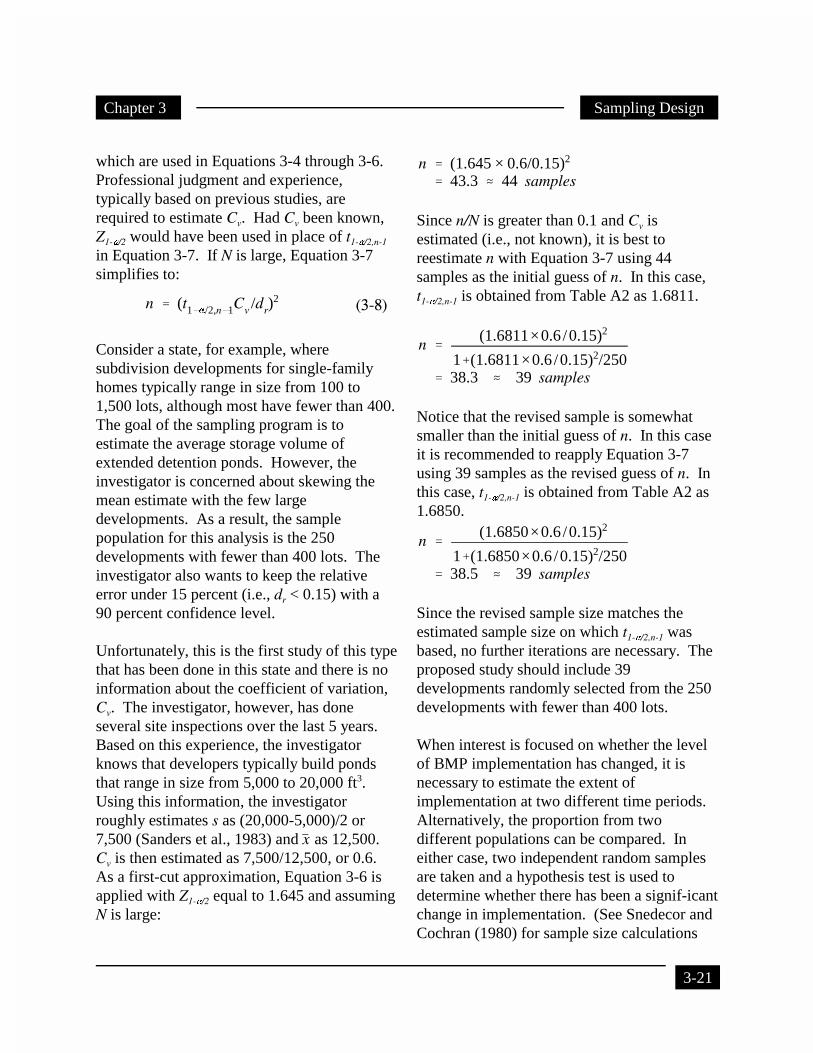
Sampling DesignChapter 3
3-21
n � (t1�/2,n1Cv /dr)2
�����
which are used in Equations 3-4 through 3-6. Professional judgment and experience,typically based on previous studies, arerequired to estimate Cv. Had Cv been known,Z1-�/2 would have been used in place of t1-�/2,n-1
in Equation 3-7. If N is large, Equation 3-7simplifies to:
Consider a state, for example, wheresubdivision developments for single-familyhomes typically range in size from 100 to1,500 lots, although most have fewer than 400. The goal of the sampling program is toestimate the average storage volume ofextended detention ponds. However, theinvestigator is concerned about skewing themean estimate with the few largedevelopments. As a result, the samplepopulation for this analysis is the 250developments with fewer than 400 lots. Theinvestigator also wants to keep the relativeerror under 15 percent (i.e., dr < 0.15) with a90 percent confidence level.
Unfortunately, this is the first study of this typethat has been done in this state and there is noinformation about the coefficient of variation,Cv. The investigator, however, has doneseveral site inspections over the last 5 years. Based on this experience, the investigatorknows that developers typically build pondsthat range in size from 5,000 to 20,000 ft3. Using this information, the investigatorroughly estimates s as (20,000-5,000)/2 or7,500 (Sanders et al., 1983) and x� as 12,500. Cv is then estimated as 7,500/12,500, or 0.6. As a first-cut approximation, Equation 3-6 isapplied with Z1-�/2 equal to 1.645 and assumingN is large:
n � (1.645 × 0.6/0.15)2
� 43.3 � 44 samples
Since n/N is greater than 0.1 and Cv isestimated (i.e., not known), it is best toreestimate n with Equation 3-7 using 44samples as the initial guess of n. In this case,t1-�/2,n-1 is obtained from Table A2 as 1.6811.
n �(1.6811×0.6 /0.15)2
1�(1.6811×0.6 /0.15)2/250� 38.3 � 39 samples
Notice that the revised sample is somewhatsmaller than the initial guess of n. In this caseit is recommended to reapply Equation 3-7using 39 samples as the revised guess of n. Inthis case, t1-�/2,n-1 is obtained from Table A2 as1.6850.
n �(1.6850×0.6 /0.15)2
1�(1.6850×0.6 /0.15)2/250� 38.5 � 39 samples
Since the revised sample size matches theestimated sample size on which t1-�/2,n-1 wasbased, no further iterations are necessary. Theproposed study should include 39developments randomly selected from the 250developments with fewer than 400 lots.
When interest is focused on whether the levelof BMP implementation has changed, it isnecessary to estimate the extent ofimplementation at two different time periods. Alternatively, the proportion from twodifferent populations can be compared. Ineither case, two independent random samplesare taken and a hypothesis test is used todetermine whether there has been a signif-icantchange in implementation. (See Snedecor andCochran (1980) for sample size calculations

Sampling Design Chapter 3
3-22
Power,1-��
�� for One-sided Test �� for Two-sided Test
0.01 0.05 0.10 0.01 0.05 0.10
0.80 10.04 6.18 4.51 11.68 7.85 6.18
0.85 11.31 7.19 5.37 13.05 8.98 7.19
0.90 13.02 8.56 6.57 14.88 10.51 8.56
0.95 15.77 10.82 8.56 17.81 12.99 10.82
0.99 21.65 15.77 13.02 24.03 18.37 15.77
Table 3-5. Common values of (Z� + Z2�)
2 for estimating sample size for use withequations 3-9 and 3-10.
no � (Z��Z2�)
2(p1q1�p2q2)
(p2�p1)2 �����
What sample size is necessary to determinewhether there is a 20 percent difference inhousehold hazardous waste disposal beforeand after an education program?
What sample size is necessary to detect adifference of 2,000 ft3 per acre of imperviousarea in average pond storage volumebetween land owners that plan and developtheir own land versus those that hireindependent consultants?
no � 10.51[(0.4)(0.6)� (0.6)(0.4)]
(0.6�0.4)2
� 126.1
for matched data.) Consider an example inwhich the proportion of house-holds thatproperly dispose of household hazardous wastewill be estimated at two time periods. Whatsample size is needed?
To compute sample sizes for comparing twoproportions, p1 and p2, it is necessary toprovide a best estimate for p1 and p2, as well asspecifying the significance level and power (1-
�). Recall that power is equal to theprobability of rejecting Ho when Ho is false. Given this information, the analyst substitutesthese values into (Snedecor and Cochran,1980) where Z
� and Z2� correspond to the
normal deviate. Although this equationassumes that N large, it is acceptable forpractical use (Snedecor and Cochran, 1980). Common values of (Z
� and Z2� )
2 aresummarized in Table 3-5. To account for p1
and p2 being estimated, Z could be substitutedwith t. In lieu of an iterative calculation,
Snedecor and Cochran (1980) propose thefollowing approach: (1) compute no usingEquation 3-9; (2) round no up to the nexthighest integer, f; and (3) multiply no by(f+3)/(f+1) to derive the final estimate of n.
To detect a difference in proportions of 0.20with a two-sided test, � equal to 0.05, 1-�equal to 0.90, and an estimate of p1 and p2
equal to 0.4 and 0.6, no is computed as

Sampling DesignChapter 3
3-23
no � (Z��Z2�)
2(s 2
1 �s 22 )
�2���� �
no � 10.51(7,5002
�7,5002)
40002
� 73.9������
What sample size is necessary to estimatethe average number of households thatcarefully monitor their fertilizer applicationswhen there is a wide variety of lawn sizes?
x̄st � �L
h1Wh x̄h ������
Rounding 126.1 to the next highest integer, f isequal to 127, and n is computed as 126.1 x130/128 or 128.1. Therefore 129 samples ineach random sample, or 258 total samples, areneeded to detect a difference in proportions of0.2. Beware of other sources of informationthat give significantly lower estimates ofsample size. In some cases the other sourcesdo not specify 1-�; otherwise, be sure that an“apples-to-apples” comparison is being made.
To compare the average from two randomsamples to detect a change of � (i.e., x
_2-x
_1), the
following equation is used:
Common values of (Z� and Z2� )
2 aresummarized in Table 3-5. To account for s1
and s2 being estimated, Z should be replacedwith t. In lieu of an iterative calculation,Snedecor and Cochran (1980) propose thefollowing approach: (1) compute no usingEquation 3-10; (2) round no up to the nexthighest integer, f; and (3) multiply no by(f+3)/(f+1) to derive the final estimate of n.
Continuing the extended detention pondexample, where s was estimated as 7,500 ft3,the investigator will also want to compare theaverage pond size between land owners thatplan and develop their own land versus thosethat hire independent consultants. Theinvestigator believes that it will be necessaryto detect a 4,000 ft3 difference to make animpact on planning decisions. Although thestandard deviation might differ between thetwo groups, there is no particular reason topropose a different s at this point. To detect adifference of 4,000 ft3 with a two-sided test, �
equal to 0.05, 1-� equal to 0.90, and anestimate of s1 and s2 equal to 7,500, no iscomputed as
Rounding 73.9 to the next highest integer, f isequal to 74, and n is computed as 73.9 x77/75 or 75.9. Therefore, 76 samplesin each random sample, or 152 totalsamples, are needed to detect adif ference of 4,000 ft3.
3.3.2 Stratified Random Sampling
The key reason for selecting a stratifiedrandom sampling strategy over simple randomsampling is to divide a heterogeneouspopulation into more homogeneous groups. Ifpopulations are grouped based on size (e.g.,lawn size) when there is a large number ofsmall units and a few larger units, a large gainin precision can be expected (Snedecor andCochran, 1980). Stratifying also allows theinvestigator to efficiently allocate samplingresources based on cost. Information frompreliminary studies (see Section 3.3) canprovide useful sampling cost information. Thestratum mean, x
_h, is computed using the
standard approach for estimating the mean.
The overall mean, x_
st, is computed as
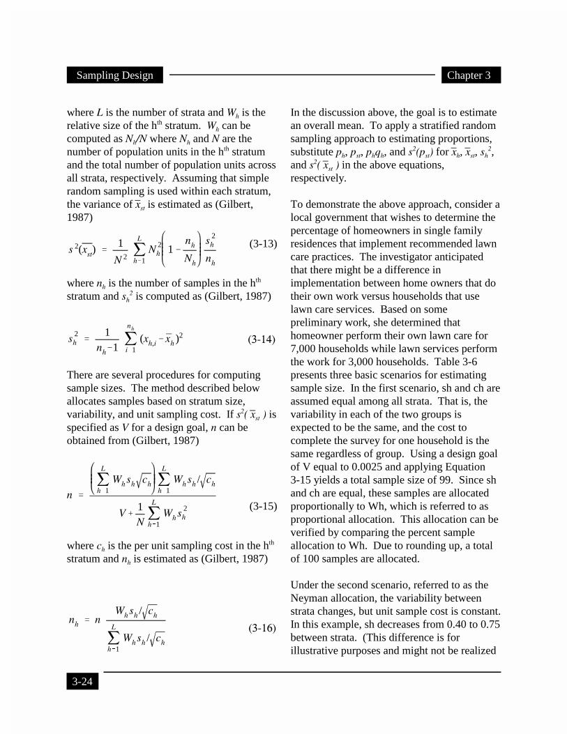
Sampling Design Chapter 3
3-24
s 2(xst) �1
N 2 �L
h1N 2
h 1�nh
Nh
s 2h
nh
s 2h �
1nh�1 �
nh
i1(xh,i� x̄h )2
������
n �
�L
h1Wh sh ch �
L
h1Wh sh / ch
V�1N �
L
h1Wh s 2
h
nh � nWh sh / ch
�L
h1Wh sh / ch
�����
where L is the number of strata and Wh is therelative size of the hth stratum. Wh can becomputed as Nh/N where Nh and N are thenumber of population units in the hth stratumand the total number of population units acrossall strata, respectively. Assuming that simplerandom sampling is used within each stratum,the variance of x
_st is estimated as (Gilbert,
1987)
(3-13)
where nh is the number of samples in the hth
stratum and sh2 is computed as (Gilbert, 1987)
There are several procedures for computingsample sizes. The method described belowallocates samples based on stratum size,variability, and unit sampling cost. If s2( x
_st ) is
specified as V for a design goal, n can beobtained from (Gilbert, 1987)
(3-15)
where ch is the per unit sampling cost in the hth
stratum and nh is estimated as (Gilbert, 1987)
In the discussion above, the goal is to estimatean overall mean. To apply a stratified randomsampling approach to estimating proportions,substitute ph, pst, phqh, and s2(pst) for x
_h, x
_st, sh
2,and s2( x
_st ) in the above equations,
respectively.
To demonstrate the above approach, consider alocal government that wishes to determine thepercentage of homeowners in single familyresidences that implement recommended lawncare practices. The investigator anticipatedthat there might be a difference inimplementation between home owners that dotheir own work versus households that uselawn care services. Based on somepreliminary work, she determined thathomeowner perform their own lawn care for7,000 households while lawn services performthe work for 3,000 households. Table 3-6presents three basic scenarios for estimatingsample size. In the first scenario, sh and ch areassumed equal among all strata. That is, thevariability in each of the two groups isexpected to be the same, and the cost tocomplete the survey for one household is thesame regardless of group. Using a design goalof V equal to 0.0025 and applying Equation3-15 yields a total sample size of 99. Since shand ch are equal, these samples are allocatedproportionally to Wh, which is referred to asproportional allocation. This allocation can beverified by comparing the percent sampleallocation to Wh. Due to rounding up, a totalof 100 samples are allocated.
Under the second scenario, referred to as theNeyman allocation, the variability betweenstrata changes, but unit sample cost is constant. In this example, sh decreases from 0.40 to 0.75between strata. (This difference is forillustrative purposes and might not be realized

Sampling DesignChapter 3
3-25
WhoProvides
Lawn Care
Numberof Lots
(Nh)
RelativeSize(Wh)
StandardDeviation
(sh)
UnitSample
Cost(ch)
Sample Allocation
Number %
A) Proportional allocation (sh and ch are constant)
Homeowner 7,000 0.70 0.50 1 70 70.0
LawnService
3,000 0.30 0.50 1 30 30.0
Using Equation 3-15, n is equal to 99.0. Applying Equation 3-16 to each stratum yields atotal of 100 samples after rounding up to the next integer.
B) Neyman allocation (ch is constant)
Homeowner 7,000 0.70 0.40 1 56 55.4
LawnService
3,000 0.30 0.75 1 45 44.6
Using Equation 3-15, n is equal to 100.9. Applying Equation 3-16 to each stratum yields atotal of 101 samples after rounding up to the next integer.
C) Allocation where sh and ch are not constant
Homeowner 7,000 0.70 0.40 1 62 60.2
LawnService
3,000 0.30 0.75 1.5 41 39.8
Using Equation 3-15, n is equal to 101.9. Applying Equation 3-16 to each stratum yields atotal of 103 samples after rounding up to the next integer.
Table 3-6. Allocation of samples.
in practice.) The total number of samplesremained roughly the same; however, anincreased number of samples are required forlawn care services. Using proportionalallocation 30 percent of the samples are takenfrom households that use lawn care serviceswhereas approximately 44.6 percent of thesamples are taken in the same stratum usingthe Neyman allocation.
Finally, introducing sample cost variation willalso affect sample allocation. In the lastscenario it was assumed that it is 50 percentmore expensive to evaluate a lot from thestratum that corresponds to the households thatuse lawn care services. (This difference is forillustrative purposes and might not be realizedin practice.) In this example, roughly the sametotal number of samples are needed to meet thedesign goal, yet fewer samples are now
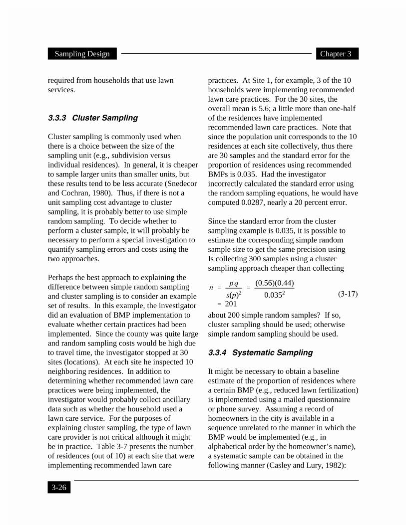
Sampling Design Chapter 3
3-26
n �pq
s(p)2�
(0.56)(0.44)
0.0352
� 201�����
required from households that use lawnservices.
3.3.3 Cluster Sampling
Cluster sampling is commonly used whenthere is a choice between the size of thesampling unit (e.g., subdivision versusindividual residences). In general, it is cheaperto sample larger units than smaller units, butthese results tend to be less accurate (Snedecorand Cochran, 1980). Thus, if there is not aunit sampling cost advantage to clustersampling, it is probably better to use simplerandom sampling. To decide whether toperform a cluster sample, it will probably benecessary to perform a special investigation toquantify sampling errors and costs using thetwo approaches.
Perhaps the best approach to explaining thedifference between simple random samplingand cluster sampling is to consider an exampleset of results. In this example, the investigatordid an evaluation of BMP implementation toevaluate whether certain practices had beenimplemented. Since the county was quite largeand random sampling costs would be high dueto travel time, the investigator stopped at 30sites (locations). At each site he inspected 10neighboring residences. In addition todetermining whether recommended lawn carepractices were being implemented, theinvestigator would probably collect ancillarydata such as whether the household used alawn care service. For the purposes ofexplaining cluster sampling, the type of lawncare provider is not critical although it mightbe in practice. Table 3-7 presents the numberof residences (out of 10) at each site that wereimplementing recommended lawn care
practices. At Site 1, for example, 3 of the 10households were implementing recommendedlawn care practices. For the 30 sites, theoverall mean is 5.6; a little more than one-halfof the residences have implementedrecommended lawn care practices. Note thatsince the population unit corresponds to the 10residences at each site collectively, thus thereare 30 samples and the standard error for theproportion of residences using recommendedBMPs is 0.035. Had the investigatorincorrectly calculated the standard error usingthe random sampling equations, he would havecomputed 0.0287, nearly a 20 percent error.
Since the standard error from the clustersampling example is 0.035, it is possible toestimate the corresponding simple randomsample size to get the same precision usingIs collecting 300 samples using a clustersampling approach cheaper than collecting
about 200 simple random samples? If so,cluster sampling should be used; otherwisesimple random sampling should be used.
3.3.4 Systematic Sampling
It might be necessary to obtain a baselineestimate of the proportion of residences wherea certain BMP (e.g., reduced lawn fertilization)is implemented using a mailed questionnaireor phone survey. Assuming a record ofhomeowners in the city is available in asequence unrelated to the manner in which theBMP would be implemented (e.g., inalphabetical order by the homeowner’s name),a systematic sample can be obtained in thefollowing manner (Casley and Lury, 1982):

Sampling DesignChapter 3
3-27
Site 1: 3a Site 2: 9 Site 3: 5 Site 4: 7 Site 5: 6 Site 6: 4
Site 7: 6 Site 8: 3 Site 9: 5 Site 10: 5 Site 11: 5 Site 12: 7
Site 13: 7 Site 14: 4 Site 15: 7 Site 16: 5 Site 17: 3 Site 18: 8
Site 19: 4 Site 20: 6 Site 21: 8 Site 22: 4 Site 23: 7 Site 24: 4
Site 25: 5 Site 26: 3 Site 27: 3 Site 28: 9 Site 29: 9 Site 30: 7
Grand Total = 168 (i.e., 168 of 300residents used recommended lawn carepractices)x_
= 5.6 (i.e., 5.6 out of 10 residents usedrecommended lawn care practices)s = 1.923
p = 5.6/10 = 0.560
s’ = 1.923/10 = 0.1923
Standard error using cluster sampling: s(p) = 0.1923/(30)0.5 = 0.035Standard error if simple random sampling assumption had been incorrectly used: s(p) = ((0.56)(1-0.56)/300)0.5 = 0.0287
a At Site 1, for example, 3 of the 10 households were implementing recommended lawn care practices.
Table 3-7. Number of residences at each site implementing recommended lawn carepractices (10 residences inspected at each site).
1. Select a random number r between 1 andn, where n is the number required in thesample.
2. The sampling units are then r, r + (N/n), r+ (2N/n), ..., r + (n-1)(N/n), where N istotal number of available records.
If the population units are in random order(e.g., no trends, no natural strata,uncorrelated), systematic sampling is, onaverage, equivalent to simple randomsampling.
Once the sampling units (in this case, specificresidences) have been selected, questionnairescan be mailed to homeowners or telephoneinquiries made about lawn care practices beingfollowed by the homeowners.
3.3.5 Concluding Remarks
In the previous examples the type of questionsasked where generally similar yet dramaticallydifferent sample sizes were developed. Thisprobably leaves the reader wondering whichone to choose. Clearly simple randomsampling is the easiest, but might very wellleave the investigator with numerousunanswered questions. The primary basis forselecting a design approach should be based ona careful review of study objectives and thediscussion in Section 3.1.2 and Table 3-1. Asshown in Section 3.3.3, cluster sampling canbe a good alternative to simple randomsampling when you can demonstrate asampling cost savings. In both cases, there isno stratification or optimization based on youra priori knowledge about patterns or sampling

Sampling Design Chapter 3
3-28
costs in the target population. When there arecritical factors that you are examining or youknow that there are group differences amongthe target population, stratified sampling(Section 3.3.2) should be used to optimize (ina less-variance sense) the precision of
population totals. On the other hand if yourobjective is to compare implementation amongtwo groups, then sample size calculationsderived from the Equations 3-9 or 3-10(Section 3.3.1) should be used.

4-1
CHAPTER 4. METHODS FOR EVALUATING DATA
4.1 INTRODUCTION
Once data have been collected, it is necessaryto statistically summarize and analyze the data. EPA recommends that the data analysismethods be selected before collecting the firstsample. Many statistical methods have beencomputerized in easy-to-use software that isavailable for use on personal computers. Inclusion or exclusion in this section does notimply an endorsement or lack thereof by theEPA. Commercial off-the-shelf software thatcovers a wide range of statistical and graphicalsupport includes SAS, Statistica, Statgraphics,Systat, Data Desk (Macintosh only), BMDP,and JMP. Numerous spreadsheets, databasemanagement packages, and other graphicssoftware can also be used to perform many ofthe needed analyses. In addition, the followingprograms, written specifically forenvironmental analyses, are also available:
• SCOUT: A Data Analysis Program, EPA,NTIS Order Number PB93-505303.
• WQHYDRO (WATERQUALITY/HYDROLOGYGRAPHICS/ANALYSIS SYSTEM), EricR. Aroner, Environmental Engineer, P.O.Box 18149, Portland, OR 97218.
• WQSTAT, Jim C. Loftis, Department ofChemical and Bioresource Engineering,Colorado State University, Fort Collins,CO 80524.
Computing the proportion of construction sitesimplementing a certain BMP or the averagestorage volume per acre of impervious area ofextended detention ponds follows directlyfrom the equations presented in Section 3.3and the equations are not repeated here. Theremainder of this section is focused onevaluating changes in BMP implementation. The methods provided in this section provideonly a cursory overview of the type of analysesthat might be of interest. For a more thoroughdiscussion on these methods, the reader isreferred to Gilbert (1987), Snedecor andCochran (1980), and Helsel and Hirsch (1995). Typically, the data collected for evaluatingchanges will typically come as two or moresets of random samples. In this case, theanalyst will test for a shift or step change.
Depending on the objective, it is appropriate toselect a one- or two-sided test. For example, ifthe analyst knows that BMP implementationwill only go up as a result of a regulatory oreducational program, a one-sided test could beformulated. Alternatively, if the analyst doesnot know whether implementation will go upor down, a two-sided test is necessary. Tosimply compare two random samples to decideif they are significantly different, a two-sidedtest is used. Typical null hypotheses (Ho) andalternative hypotheses (Ha) for one- and two-sided tests are provided below:

Methods for Evaluating Data Chapter 4
4-2
Tests for Two Independent Random Samples
Test* Key Assumptions
Two-sample t • Both data sets must be normally distributed• Data sets should have equal variances†
Mann-Whitney • None
* The standard forms of these tests requireindependent random samples.
† The variance homogeneity assumption canbe relaxed.
t `(x1 ` x2 ) ` �0
sp1n1
` 1n2
(4-1)
sp `s 2
1 (n1` 1) ` s 22 (n2` 1)
n1 ` n2 ` 2
0.5
(4-2)
One-sided testHo: BMP Implementation (Post regulation) �
BMP Implementation (Pre regulation)
Ha: BMP Implementation (Post regulation) >BMP Implementation (Pre regulation)
Two-sided testHo: BMP Implementation (Post education
program) = BMP Implementation (Preeducation program)
Ha: BMP Implementation (Post educationprogram) � BMP Implementation (Preeducation program)
Selecting a one-sided test instead of a two-sided test results in an increased power for thesame significance level (Winer, 1971). Thatis, if the conditions are appropriate, acorresponding one-sided test is more desirablethan a two-sided test given the same � andsample size. The manager and analyst shouldtake great care in selecting one- or two-sidedtests.
4.2 COMPARING THE MEANS FROM TWOINDEPENDENT RANDOM SAMPLES
The Student’s t test for two samples and theMann-Whitney test are the most appropriatetests for these types of data. Assuming thedata meet the assumptions of the t test, thetwo-sample t statistic with n1+n2-2 degrees offreedom is (Remington and Schork, 1970)
where n1 and n2 are the sample size of the firstand second data set and x1
_and x2
_are the
estimated means from the first and second dataset, respectively. The pooled standarddeviation, sp, is defined by
where s12 and s2
2 correspond to the estimatedvariances of the first and second data set,respectively. The difference quantity (�o) canbe any value, but here it is set to zero. �o canbe set to a non-zero value to test whether thedifference between the two data sets is greaterthan a selected value. If the variances are notequal, refer to Snedecor and Cochran (1980)for methods for computing the t statistic. In atwo-sided test, the value from Equation 4-1 iscompared to the t value from Table A2 with�/2 and n1+n2-2 degrees of freedom.
The Mann-Whitney test can also be used tocompare two independent random samples. This test is very flexible since there are noassumptions about the distribution of eithersample or whether the distributions have to bethe same (Helsel and Hirsch, 1995). Wilcoxon(1945) first introduced this test for equal-sized
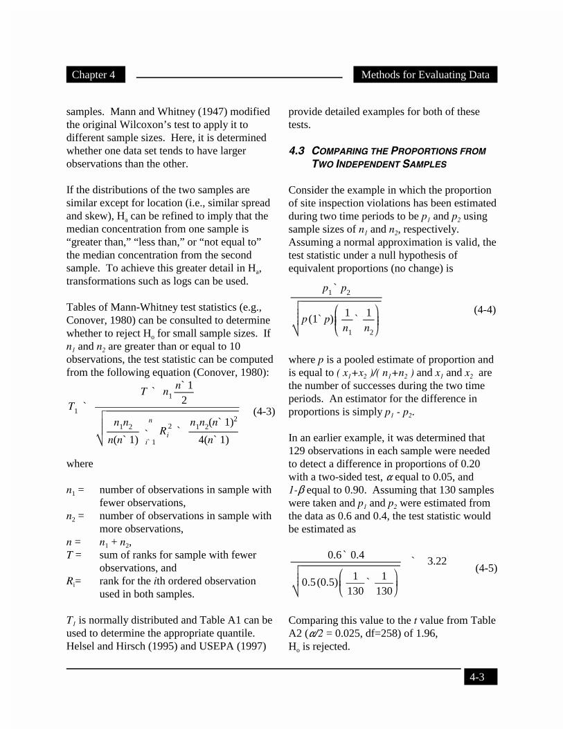
Chapter 4 Methods for Evaluating Data
4-3
T1 `T ` n1
n` 12
n1n2
n(n` 1) `n
i` 1R 2
i `n1n2(n` 1)2
4(n` 1)
p1 ` p2
p (1` p)1n1
`1n2
(4-4)
0.6` 0.4
0.5(0.5) 1130
` 1130
` 3.22
samples. Mann and Whitney (1947) modifiedthe original Wilcoxon’s test to apply it todifferent sample sizes. Here, it is determinedwhether one data set tends to have largerobservations than the other.
If the distributions of the two samples aresimilar except for location (i.e., similar spreadand skew), Ha can be refined to imply that themedian concentration from one sample is“greater than,” “less than,” or “not equal to”the median concentration from the secondsample. To achieve this greater detail in Ha,transformations such as logs can be used.
Tables of Mann-Whitney test statistics (e.g.,Conover, 1980) can be consulted to determinewhether to reject Ho for small sample sizes. Ifn1 and n2 are greater than or equal to 10observations, the test statistic can be computedfrom the following equation (Conover, 1980):
(4-3)
where
n1 = number of observations in sample withfewer observations,
n2 = number of observations in sample withmore observations,
n = n1 + n2,T = sum of ranks for sample with fewer
observations, andRi= rank for the ith ordered observation
used in both samples.
T1 is normally distributed and Table A1 can beused to determine the appropriate quantile. Helsel and Hirsch (1995) and USEPA (1997)
provide detailed examples for both of thesetests.
4.3 COMPARING THE PROPORTIONS FROMTWO INDEPENDENT SAMPLES
Consider the example in which the proportionof site inspection violations has been estimatedduring two time periods to be p1 and p2 usingsample sizes of n1 and n2, respectively. Assuming a normal approximation is valid, thetest statistic under a null hypothesis ofequivalent proportions (no change) is
where p is a pooled estimate of proportion andis equal to ( x1+x2 )/( n1+n2 ) and x1 and x2 arethe number of successes during the two timeperiods. An estimator for the difference inproportions is simply p1 - p2.
In an earlier example, it was determined that129 observations in each sample were neededto detect a difference in proportions of 0.20with a two-sided test, � equal to 0.05, and 1-� equal to 0.90. Assuming that 130 sampleswere taken and p1 and p2 were estimated fromthe data as 0.6 and 0.4, the test statistic wouldbe estimated as
(4-5)
Comparing this value to the t value from TableA2 (�/2 = 0.025, df=258) of 1.96, Ho is rejected.

Methods for Evaluating Data Chapter 4
4-4
�ct ` `m
i` 1`
k
j` 1
(Oij ` Eij)2
Eij
(4-6)
4.4 COMPARING MORE THAN TWOINDEPENDENT RANDOM SAMPLES
The analysis of variance (ANOVA) andKruskal-Wallis are extensions of thetwo-sample t and Mann-Whitney tests,respectively, and can be used for analyzingmore than two independent random sampleswhen the data are continuous (e.g., meanacreage). Unlike the t test described earlier,the ANOVA can have more than one factor orexplanatory variable. The Kruskal-Wallis testaccommodates only one factor, whereas theFriedman test can be used for two factors. Inaddition to applying one of the above tests todetermine if one of the samples is significantlydifferent from the others, it is also necessary todo postevaluations to determine which of thesamples is different. This section recommendsTukey’s method to analyze the raw or rank-transformed data only if one of the previoustests (ANOVA, rank-transformed ANOVA,Kruskal-Wallis, Friedman) indicates asignificant difference between groups. Tukey’s method can be used for equal orunequal sample sizes (Helsel and Hirsch,1995). The reader is cautioned, whenperforming an ANOVA using standardsoftware, to be sure that the ANOVA test usedmatches the data. See USEPA (1997) for amore detailed discussion on comparing morethan two independent random samples.
4.5 COMPARING CATEGORICAL DATA
In comparing categorical data, it is importantto distinguish between nominal categories(e.g., land ownership, county location, type ofBMP) and ordinal categories (e.g., BMPimplementation rankings, low-medium-highscales).
The starting point for all evaluations is thedevelopment of a contingency table. In Table4-1, the preference of three BMPs is comparedto resident type in a contingency table. In thiscase both categorical variables are nominal. Inthis example, 45 of the 102 residents that ownthe house they occupy used BMP1. There werea total of 174 observations.
To test for independence, the sum of thesquared differences between the expected (Eij)and the observed (Oij) count summed over allcells is computed as (Helsel and Hirsch, 1995)
where Eij is equal to AiCj/N. �ct is compared tothe 1-� quantile of the �2 distribution with(m-1)(k-1) degrees of freedom (see Table A3).
In the example presented in Table 4-1, thesymbols listed in the parentheses correspond tothe above equation. Note that k corresponds tothe three types of BMPs and m corresponds tothe three different types of residents. Table 4-2 shows computed values of Eij and(Oij-Eij)
2/Eij) in parentheses for the exampledata. �ct is equal to 14.60. From Table A3, the0.95 quantile of the �2 distribution with 4degrees of freedom is 9.488. Ho is rejected;the selection of BMP is not random among thedifferent resident types. The largest values inthe parentheses in Table 4-2 give an idea as towhich combinations of resident type and BMPare noteworthy. In this example, it appearsthat BMP2 is preferred to BMP1 for thoseresidents that rent the house they occupy.

Chapter 4 Methods for Evaluating Data
4-5
Table 4-1. Contingency table of observed resident type and implemented BMP.
Resident Type BMP1 BMP2 BMP3 Row Total,
Ai
Rent 10 (O11) 30 (O12) 17 (O13) 57 (A1)
Own 45 (O21) 32 (O22) 25 (O23) 102 (A2)
Seasonal 8 (O31) 3 (O32) 4 (O33) 15 (A3)
Column Total, Cj 63 (C1) 65 (C2) 46 (C3) 174 (N)
Key to Symbols:Oij = number of observations for the ith resident and jth BMP typeAi = row total for the ith resident type (total number of observations for a given resident type)Cj = column total for the jth BMP type (total number of observations for a given BMP type)N = total number of observations
Table 4-2. Contingency table of expected resident type and implemented BMP.(Values in parentheses correspond to (Oij-Eij)
2/Eij.)
Resident Type BMP1 BMP2 BMP3 Row Total
Rent 20.64(5.48)
21.29(3.56)
15.07(0.25)
57
Own 36.93(1.76)
38.10(0.98)
26.97(0.14)
102
Seasonal 5.43(1.22)
5.60(1.21)
3.97(0.00)
15
Column Total 63 65 46 174
Rx ` `x` 1
i` 1Ai ` (Ax` 1)/2 (4-7)
Dj ``m
i` 1Oij Ri
Cj
(4-8)
Now consider that in addition to evaluatinginformation regarding the resident and BMPtype, we also recorded a value from 1 to 5indicating how well the BMP was installed andmaintained, with 5 indicating the best results. In this case, the BMP implementation rating isordinal. Using the same notation as before, theaverage rank of observations in row x, Rx, isequal to (Helsel and Hirsch, 1995)
where Ai corresponds to the row total. Theaverage rank of observations in column j, Dj, isequal to

Methods for Evaluating Data Chapter 4
4-6
K ` (N ` 1)`
k
j` 1Cj D
2j ` N N` 1
N
2
`m
i` 1Ai R
2i ` N
N` 1N
2
Table 4-3. Contingency table of implemented BMP and rating of installation andmaintenance.
BMPImplementation
Rating BMP1 BMP2 BMP3 Row Total,
Ai
1 1 (O11) 2 (O12) 2 (O13) 5 (A1)
2 7 (O21) 3 (O22) 5 (O23) 15 (A2)
3 15 (O31) 16 (O32) 26 (O33) 57 (A3)
4 32 (O41) 29 (O42) 9 (O43) 70 (A4)
5 8 (O51) 15 (O52) 4 (O53) 27 (A5)
Column Total, Cj 63 (C1) 65 (C2) 46 (C3) 174 (N)
Key to Symbols:Oij = number of observations for the ith BMP implementation rating and jth BMP typeAi = row total for the ith BMP implementation rating (total number of observations for a given BMP implementation rating)Cj = column total for the jth BMP type (total number of observations for a given BMP type)N = total number of observations
�b `S
12
(N 2 ` SSa)(N2 ` SSb)
(4-10)
where Cj corresponds to the column total. TheKruskal-Wallis test statistic is then computedas
(4-9)
where K is compared to the �2 distribution withk-1 degrees of freedom. This is the mostgeneral form of the Kruskal-Wallis test since itis a comparison of distribution shifts rather thanshifts in the median (Helsel and Hirsch, 1995).
Table 4-3 is a continuation of the previousexample indicating the BMP implementationrating for each BMP type. For example, 29 ofthe 70 observations that were given a rating of4 are associated with BMP2. The terms insidethe parentheses of Table 4-3 correspond to the
terms used in Equations 4-7 to 4-9. Note that kcorresponds to the three types of BMPs and mcorresponds to the five different levels of BMPimplementation. Using Equation 4-9 for thedata in Table 4-3, K is equal to 14.86. Comparing this value to 5.991 obtained fromTable A3, there is a significant difference inthe quality of implementation between thethree BMPs.
The last type of categorical data evaluationconsidered in this chapter is when bothvariables are ordinal. The Kendall �b fortieddata can be used for this analysis. Thestatistic �b is calculated as (Helsel and Hirsch,1995)

Chapter 4 Methods for Evaluating Data
4-7
S ` `allxy
`i>x
`j>y
OxyOij ` `i<x
`j<
SSa ` `m
i` 1A 2
i (4-12)
SSc ` `k
j` 1C 2
j ������
Table 4-4. Contingency table of implemented BMP and sample year.
BMPImplementation
Rating Year 1 Year 2 Year 3Row Total,
Ai ai
1 2 (O11) 1 (O12) 2 (O13) 5 (A1) 0.029
2 5 (O21) 7 (O22) 3 (O23) 15 (A2) 0.086
3 26 (O31) 15 (O32) 16 (O33) 57 (A3) 0.328
4 9 (O41) 32 (O42) 29 (O43) 70 (A4) 0.402
5 4 (O51) 8 (O52) 15 (O53) 27 (A5) 0.155
Column Total, Cj 46 (C1) 63 (C2) 65 (C3) 174 (N)
cj 0.264 0.362 0.374
Key to Symbols:Oij = number of observations for the ith BMP implementation rating and jth yearAi = row total for the ith BMP implementation rating (total number of observations for a given BMP implementation rating)Cj = column total for the jth BMP type (total number of observations for a given year)N = total number of observationsai = Ai /Ncj = Cj /N
ZS `
S` 1�S
if S>0
S` 1�S
if S<0(4-14)
�s `N 3
91` `
m
i` 1a 3
i 1` `k
j` 1
where S, SSa, and SSc are computed as
(4-11)
To determine whether �b is significant, S ismodified to a normal statistic using
where
(4-15)
where ZS is zero if S is zero. The values of ai
and ci are computed as Ai /N and Ci /N,respectively.
Table 4-4 presents the BMP implementationratings that were taken in three separate years. For example, 15 of the 57 observations thatwere given a rating of 3 are associated withYear 2. Using Equations 4-11 and 4-15, S and�s are equal to 2,509 and 679.75, respectively. Therefore, Zs is equal to (2509-1)/679.75 or3.69. Comparing this value to a value of 1.96obtained from Table A1 (�/2=0.025) indicatesthat BMP implementation is improving withtime.

Methods for Evaluating Data Chapter 4
4-8

5-1
CHAPTER 5. CONDUCTING THE EVALUATION
5.1 INTRODUCTION
This chapter addresses the process ofdetermining whether urban MMs or BMPs arebeing implemented and whether they are beingimplemented according to approved standardsor specifications. Guidance is provided onwhat should be measured to assess MM andBMP implementation, as well as methods forcollecting the information, including physicalsite evaluations, mail- and/or telephone-basedsurveys, personal interviews, and aerialreconnaissance and photography. Designingsurvey instruments to avoid error and ratingMM and BMP implementation are alsodiscussed.
Evaluation methods are separated into twotypes: Expert evaluations and self-evaluations. Expert evaluations are those in which actualsite investigations are conducted by trainedpersonnel to gather information on MM orBMP implementation. Self-evaluations arethose in which answers to a predesignedquestionnaire or survey are provided by theperson being surveyed, for example a localgovernment representative or homeowner (seeExample). The answers provided are used assurvey results. Self-evaluations might alsoinclude examination of materials related to asite, such as permit applications or inspectionreports. Extreme caution should be exercisedwhen using data from self-evaluations as thebasis for assessing MM or BMP compliancesince they are not typically reliable for thispurpose (i.e., most people will not reportfailure or non-compliance). Each of theseevaluation methods has advantages anddisadvantages that should be considered prior
to deciding which one to use or in whatcombination to use them. Aerialreconnaissance and photography can be usedto support either evaluation method.
Self-evaluations are useful for collectinginformation on the level of awareness thatresidents, developers, or local governmentrepresentatives of have of MMs or BMPs,dates of BMP implementation or inspection,soil conditions, which MMs or BMPs wereimplemented, and whether the assistance of alocal or private BMP implementationprofessional was used. However, the type ofor level of detail of information that can beobtained from self-evaluations might beinadequate to satisfy the objectives of a MM orBMP implementation survey. If this is thecase, expert evaluations might be called for. Expert evaluations are necessary if theinformation on MM or BMP implementationthat is required must be more detailed or morereliable than that that can be obtained withself-evaluations. Examples of information thatwould be obtained reliably only through anexpert evaluation include an objectiveassessment of the adequacy of MM or BMPimplementation, the degree to which site-specific factors (e.g., type of vegetative cover,soil type, or presence of a water body)influenced MM or BMP implementation, orthe need for changes in standards andspecifications for MM or BMPimplementation. Sections 5.3 and 5.4 discussexpert evaluations and self-evaluations,respectively, in more detail.

Chapter 5 Conducting the Evaluation
5-2
A survey of lawn care practices in the Westmorland neighborhood of the city of Madison,Wisconsin was conducted by telephone interviews, after advance notice was sent tohomeowners. The objectives of the survey were to:
• Determine the number of people who fertilized their lawn either themselves orthrough a professional service.
• Identify the usage of fertilizer (i.e., when it was applied and the quantity applied).• Determine the brands and types of fertilizers used.• Identify the pattern of usage of separate weed killers and insecticides.
The survey provided information on:
• The percentage of homeowners that fertilized their lawns themselves.• The demographic profile (e.g., sex, age, number of children) of the homeowners in
the area that were most likely to use a professional service.• The annual frequency of fertilizer applications.• The type of equipment used for fertilizer applications.• The percentage of homeowners who said they followed manufacturer
recommendations for fertilizer applications.• The percentage of homeowners who used fertilizer/insecticide combinations.• The percentage of homeowners that used separate weed killers and insecticides.• How the homeowners disposed of grass clippings.
Example . . . Survey of lawn care practices. (Gene Kroupa & Associates, 1995)
Other important factors to consider whenchoosing variables include the time of yearwhen the BMP compliance survey will beconducted and when BMPs were installed. Some urban BMPs, or aspects of theirimplementation that can be analyzed, vary withtime of year, phase of construction, or lengthof time after having been installed. Thetemporary controls for erosion and sedimentcontrol, for instance, would not be inspectedafter construction is complete and a site hasbeen stabilized. Variables that are appropriateto time-specific factors should be chosen. Concerning BMPs that have been in place forsome time, the adequacy of implementationmight be of less interest than the adequacy ofthe operation and maintenance of the BMP. For example, it might be of interest to inspect
bridge runoff systems for proper cleaning andmaintenance rather than to determine whetherthe number and spacing of runoff drains issufficient for the particular bridge. Ifnumerous BMPs are being analyzed during asingle site visit, variables that relate todifferent aspects of BMP installation,operation, and maintenance might be chosenseparately for each BMP to be inspected.
Aerial reconnaissance and photography isanother means available for collectinginformation on urban or watershed practices,though many of the MMs and BMPs used inurban areas might be difficult if not impossibleto identify on aerial photographs. Aerialreconnaissance and photography are discussedin detail in Section 5.5.

Conducting the Evaluation Chapter 5
5-3
The general types of information obtainablewith self-evaluations are listed in Table 5-1. Regardless of the approach(es) used, properand thorough preparation for the evaluation isthe key to success.
5.2 CHOICE OF VARIABLES
Once the objectives of a BMP implementationor compliance survey have been clearlydefined, the most important factor in theassessment of MM or BMP implementation isthe determination of which variable(s) tomeasure. A good variable provides a directmeasure of how well a BMP was or is beingimplemented. Individual variables shouldprovide measures of different factors related toBMP implementation. The best variables arethose which are measures of the adequacy ofMM or BMP implementation and are based onquantifiable expressions of conformance withstate standards and specifications. As thevariables that are used become less directlyrelated to actual MM or BMP implementation,their accuracy as measures of BMPimplementation decreases.
Examples of useful variables could include thechange in the quantity of household hazardouswaste collected or the percent of onsitedisposal systems in a subwatershed that areoperating properly, both of which would beexpressed in terms of conformance withapplicable state and/or local standards andspecifications. Less useful variables measurefactors that are related to MM and BMPimplementation but do not necessarily providean accurate measure of their implementation. Examples of these types of variables are the
number of runoff conveyance structuresconstructed in a year and the number of onsitedisposal systems approved for installation. Other poor variables would be the passage oflegislation requiring MM or BMP applicationon construction sites, development of an publicinformation program for lawn management, orthe number of requests for information onhousehold hazardous waste disposal. Although these variables relate to MM or BMPimplementation, they provide no realinformation on whether MMs or BMPs areactually being implemented or whether theyare being implemented properly.
Variables generally will not directly relate toMM implementation, as most urban MMs arecombinations of several BMPs. Measures ofMM implementation, therefore, usually will bebased on separate assessments of two or moreBMPs, and the implementation of each BMPwill be based on a unique set of variables. Some examples of BMPs related to EPA’s SiteDevelopment Management Measure, variablesfor assessing compliance with the BMPs, andrelated standards and specifications that mightbe required by local regulatory authorities arepresented in Figure 5-1. Because developersand homeowners choose to implement or notimplement MMs or BMPs based on site-specific conditions, it is also appropriate toapply varying weights to the variables chosento assess MM and BMP implementation tocorrespond to site-specific conditions. Forexample, variables related to onsite disposalsystems might be de-emphasized—and other,more applicable variables emphasizedmore—in areas where most homes are

Chapter 5 Conducting the Evaluation
5-4
Table 5-1. General types of information obtainable with self-evaluations and expertevaluations.
Information obtainable from Self-Evaluations
Background Information
• Type of development installed (e.g., residential, commercial, industrial,recreational)
• Percent impervious area• Inspection schedule• Operation and maintenance practices• Map
Management Measures / Best Management Practices
• Nonstructural practices• BMPs installed• Dates of MM / BMP installation• Design specifications of BMPs• Type of water body or area protected• Previous management measures used
ESC Plans (for construction)• Preparation of ESC plans• Dates of plan preparation and revisions• Date of initial plan implementation• Total acreage under management• Certification requirements
Information that Requires Expert Evaluations
• Design sufficiency• Installation sufficiency• Adequacy of operation / maintenance• Confirmation of information from self-evaluations

Conducting the Evaluation Chapter 5
5-5
Site Development Management Measure
Plan, design, and develop sites to:
(1) Protect areas that provide important water quality benefits and/or are particularlysusceptible to erosion and sediment loss;
(2) Limit increases of impervious areas, except where necessary;
(3) Limit land disturbance activities such as clearing and grading, and cut and fill to reduceerosion and sediment loss; and
(4) Limit disturbance of natural drainage features and vegetation.
Related BMPs, measurement variables, and standards and specifications:
Management MeasurePractice
Potential MeasurementVariable
Example Related Standardsand Specifications
· Phasing and limiting areas ofdisturbance
· Length of time disturbed arealeft without stabilization(temporary or permanent)
· Maximum time an area maybe left unstabilized
· Maximum area that may bedisturbed at one time,depending on type ofconstruction and project
· Preserving natural drainagefeatures and naturaldepressional storage areas
· Degree to whichpostdevelopment landscapepreserves predevelopmentlandscape features
· Site-specific requirements forpreservation of naturaldrainage features,determined during thepermitting process
· Minimizing imperviousness · Percent impervious surface· Percent increase in
impervious surface
· Maximum imperviousness,depending on type ofdevelopment
· Maximum percent increase inimperviousness, based ontype of development
· Minimum disturbance /minimum maintenance
· Quantity of land altered bydevelopment from itspredevelopment condition
· Guidelines for protection ofnatural vegetation and sitecharacteristics, proposed forproject during projectdevelopment
Figure 5-1. Potential variables and examples of implementation standards andspecifications that might be useful for evaluating compliance with the New DevelopmentManagement Measure.

Chapter 5 Conducting the Evaluation
5-6
connected to a sewer system. Similarly, on aconstruction site near a water body, variablesrelated to sediment runoff and chemicaldeposition (pesticide use, fertilizer use) mightbe emphasized over other variables to arrive ata site-specific rating of the adequacy of MM orBMP implementation.
The purpose for which the informationcollected during a MM or BMPimplementation survey will be used is anotherimportant consideration when selectingvariables. An implementation survey canserve many purposes beyond the primarypurpose of assessing MM and BMPimplementation. For instance, variables mightbe selected to assess compliance with eachcategory of BMP that is of interest and toassess overall compliance with BMPspecification and standards. In addition, othervariables might be selected to assess the effectthat specific circumstances have on the abilityor willingness of homeowners or developers tocomply with BMP implementation standardsor specifications. For example, the level ofparticipation in a household hazardous wastecollection program could be investigated withrespect to variables for collection locations andhours of operation. The information obtainedfrom evaluations using the latter type ofvariable could be useful for modifying MM orBMP implementation standards andspecifications for application to particulartypes of developments or site conditions.
Table 5-2 provides examples of good and poorvariables for the assessment of implementationof the urban MMs developed by EPA(USEPA, 1993a). The variables listed in thetable are only examples, and local or regionalconditions should ultimately dictate whatvariables should be used. The Center for
Watershed Protection (CWP) published areport, Environmental indicators to assessstormwater control programs and practices(Clayton and Brown, 1996), that containsadditional information on this subject. CWPalso recommended that it might be necessaryto evaluate BMP specifications to determinewhether those for “older” structural BMPs arestill appropriate for pollution prevention.
5.3 EXPERT EVALUATIONS
5.3.1 Site Evaluations
Expert evaluations are the best way to collectreliable information on MM and BMPimplementation. They involve a person orteam of people visiting individual sites andspeaking with homeowners and/or developersto obtain information on MM and BMPimplementation (see Example). For many ofthe MMs, assessing and verifying compliancewill require a site visit and evaluation. Thefollowing should be considered before expertevaluations are conducted:
• Obtaining permission of the homeowner ordeveloper. Without proper authorizationto visit a site from the homeowner ordeveloper, the relationship between theregulated community and the localregulatory authority, and any futureregulatory or compliance action, could bejeopardized.
• The type(s) of expertise needed to assessproper implementation. For some MMs, ateam of trained personnel might berequired to determine whether MMs havebeen implemented properly.

Conducting the Evaluation Chapter 5
5-7
Table 5-2. Example variables for assessing management measure implementation.
ManagementMeasure Good Variable Poor Variable
AppropriateSampling Unit
URBAN RUNOFF
New Development # Number of county staff trainedin ESC control.
# Width of filter strips relative toarea drained.
# Allocation of funding fordevelopment of educationmaterials.
# Scheduled frequency of runoffcontrol maintenance.
# Subwatershed# Development site
WatershedProtection
# Percent of highly erodiblesoils left in an undevelopedstate.
# Percent natural drainageways altered.
# Development of watershedanalysis GIS system.
# Assessed fines for violationsof setback standards.
# Subwatershed
Site Development # Ratio of area of land withstructures to total disturbedland at a development site
# Area of environmentallysensitive land to total area ofsame disturbed duringconstruction
# Number of erosion andsediment control plansdeveloped.
# Subwatershed
CONSTRUCTION ACTIVITIES
Construction SiteErosion andSediment Control(ESC)
# Distance runoff travels ondisturbed soils before it isintercepted by a runoff controldevice (relative to slope andsoil type).
# Adequacy of ESC practicesrelative to soil type, slope,and precipitation.
# Number of ESC BMPs usedat a construction site.
# Number of ESC plans written.
# Development site
Construction SiteChemical Control
# Proper installation and use ofdesignated area for chemicaland petroleum productstorage and handling.
# Proper timing and applicationrate of nutrients atdevelopment site.
# Content and quality of spillprevention and control plan.
# Number of approved nutrientmanagement plans.
# Development site
EXISTING DEVELOPMENT
ExistingDevelopment
# Proper operation andmaintenance of surface waterrunoff management facilities.
# Installation of appropriateBMPs in areas assignedpriority as being in need ofstructural NPS controls.
# Development of a schedulefor BMP implementation.
# Setting priorities for structuralimprovements in developmentareas.
# Subwatershed

Chapter 5 Conducting the Evaluation
5-8
Table 5-2. (cont.)
ManagementMeasure Good Variable Poor Variable
AppropriateSampling Unit
ONSITE DISPOSAL SYSTEMS
New OnsiteDisposal Systems
# Proper siting and installationof new OSDS.
# Density of development withOSDS in areas with nitrogen-limited waters
# Number of OSDS installed.# Reduction in garbage
disposal sales.
# Subwatershed# City# Town
Operating OnsiteDisposal Systems
# Increase in proper OSDSoperation and maintenance 6months after a publiceducation campaign.
# Average time between OSDSmaintenance visits.
# Scheduled frequency ofOSDS inspections.
# Authorization of funding forpublic education campaign onOSDS.
# Subwatershed# City# Town
POLLUTION PREVENTION
PollutionPrevention
# Increase in volume ofhousehold hazardous wastescollected.
# Miles of roads adopted forcitizen cleanup and volume oftrash collected.
# Number of licenses issued tolawn care companies offering“chemical-free” lawn care.
# Development of pollutionprevention campaigns bynongovernmentalorganizations.
# City# Town
ROADS, HIGHWAYS, AND BRIDGES
Planning, Siting,and DevelopingRoads andHighways
# Right-of-ways set aside forroads and highways based onprojected future growth, andappropriateness of land setaside for such use.
# Miles of road constructed. # Subwatershed
Bridges # Total distance of bridges inenvironmentally sensitiveareas.
# Number of bridgesconstructed.
# Subwatershed
ConstructionProjects
# Installation of ESC practicesearly in construction project.
# ESC practices installed earlyin construction project.
# Number of ESC plansprepared and approved.
# Number of ESC BMPs usedduring construction.
# Subwatershed

Conducting the Evaluation Chapter 5
5-9
In Delaware, private construction siteinspectors make at least weekly sitevisits to large or significant constructionsites. The private inspectors are trainedby the state and report violations of ESCregulations and inadequacies in ESCplans or BMP implementation to the stateor local ESC agency, the developer, andthe contractor. They also offer timely on-site technical assistance. While not acomprehensive ESC BMPimplementation inventory program, it canbe used as a model for the developmentof such a program.
Example . . . Delaware construction sitereviews.
Table 5-2. (cont.)
ManagementMeasure Good Variable Poor Variable
AppropriateSampling Unit
ROADS, HIGHWAYS, AND BRIDGES (cont.)
Construction SiteChemical Control
# Proper installation and use ofdesignated area for chemicaland petroleum productstorage and handling.
# Proper timing and applicationrate of nutrients atdevelopment site.
# Pounds of herbicide applied. # Subwatershed
Operation andMaintenance
# Operating efficiency of NPSpollution control BMPs.
# Ratio of exposed slopesand\or damaged vegetatedareas to 100 m of roadwaylength.
# Frequency of street sweeping.
# Purchase of salt applicationequipment.
# Subwatershed
Road, Highway,and Bridge RunoffSystems
# Adherence to schedule forimplementation of runoffcontrols on roadwaysdetermined to need same.
# Percent of roadwayrefurbishment projects thatinclude runoff controlimprovements on roadsneeding same.
# Purchase of land for locationof treatment facilities.
# Subwatershed
• The activities that should occur during anexpert evaluation. This information isnecessary for proper and completepreparation for the site visit, so that it can becompleted in a single visit and at the propertime.
• Inspection reports or certifications(developed during construction or as theresult of other studies) might exist for someBMPs. The team of trained personnel shouldconsider whether the BMP was built tostandards that a “new” BMP would be builtto meet the MMs. (This might requirereviewing the engineering design andspecifications.) If the standards arecomparable, then a previous inspection

Chapter 5 Conducting the Evaluation
5-10
report or certification might be acceptable inlieu of a detailed site visit and evaluation.
• The method of rating the MMs and BMPs. MM and BMP rating systems are discussedbelow.
• Consistency among evaluation teams andbetween site evaluations. Proper trainingand preparation of expert evaluation teammembers are crucial to ensure accuracy andconsistency.
• The collection of information while at a site. Information collection should be facilitatedwith preparation of data collection forms thatinclude any necessary MM and BMP ratinginformation needed by the evaluation teammembers.
• The content and format of post-evaluationdiscussions. Site evaluation team membersshould bear in mind the value ofpostevaluation discussion among teammembers. Notes can be taken during theevaluation concerning any items that wouldbenefit from group discussion.
Evaluators might consist of a single personsuitably trained in urban expert evaluation to agroup of professionals with varied expertise. The composition of evaluation teams willdepend on the types of MMs or BMPs beingevaluated. Potential team members couldinclude:
• Civil engineer• Land use planner• Hydrologist• Soil scientist• Water quality expert
The composition of evaluation teams can varydepending on the purpose of the evaluation,available staff and other resources, and thegeographic area being covered. All teammembers should be familiar with the requiredMMs and BMPs, and each team should have amember who has previously participated in anexpert evaluation. This will ensure familiaritywith the technical aspects of the MMs andBMPs that will be rated during the evaluationand the expert evaluation process.
Training might be necessary to bring all teammembers to the level of proficiency needed toconduct the expert evaluations. State or localregulatory personnel should be familiar withurban conditions, state BMP standards andspecifications, and proper BMPimplementation, and therefore are generallywell qualified to teach these topics toevaluation team members who are less familiarwith them. Local regulatory agencyrepresentatives or other specialists who haveparticipated in BMP implementation surveysmight be enlisted to train evaluation teammembers about the actual conduct of expertevaluations. This training should includeidentification of BMPs particularly critical towater quality protection, analysis of erosionpotential, and other aspects of BMPimplementation that require professionaljudgement, as well as any standard methodsfor measurements to judge BMPimplementation against state standards andspecifications.
Alternatively, if only one or two individualswill be conducting expert evaluations, theirtraining in the various specialties, such asthose listed above, necessary to evaluate thequality of MM and BMP implementationcould be provided by a team of specialists who

Conducting the Evaluation Chapter 5
5-11
are familiar with urban BMPs and nonpointsource pollution.
In the interest of consistency among theevaluations and among team members, it isadvisable that one or more mock evaluationstake place prior to visiting selected samplesites. These “practice sessions” provide teammembers with an opportunity to becomefamiliar with MMs and BMPs as they shouldbe implemented under different siteconditions, gain familiarity with the evaluationforms and meanings of the terms and questionson them, and learn from other team memberswith different expertise. Mock evaluations arevaluable for ensuring that all evaluators have asimilar understanding of the intent of thequestions, especially for questions whoseresponses involve a degree of subjectivity onthe part of the evaluator.
Where expert evaluation teams are composedof more than two or three people, it might behelpful to divide up the various responsibilitiesfor conducting the expert evaluations amongteam members ahead of time to avoidconfusion at the site and to be certain that alltasks are completed but not duplicated. Havinga spokesperson for the group who will beresponsible for communicating with thehomeowner or developer—prior to the expertevaluation, at the expert evaluation if they arepresent, and afterward—might also be helpful. A local regulatory agency representative isgenerally a good choice as spokespersonbecause he/she can represent the county ormunicipal authorities. Newly-formedevaluation teams might benefit most from adivision of labor and selection of a team leaderor team coordinator with experience in expertevaluations who will be responsible for thequality of the expert evaluations. Smaller
teams and larger teams that have experienceworking together might find that a division ofresponsibilities is not necessary. Ifresponsibilities are to be assigned, mockevaluations can be a good time to work outthese details.
5.3.2 Rating Implementation ofManagement Measures and BestManagement Practices
Many factors influence the implementation ofMMs and BMPs, so it is sometimes necessaryto use best professional judgment (BPJ) to ratetheir implementation and BPJ will almostalways be necessary when rating overall BMPcompliance at a site. Site-specific factors suchas soil type, amount of area exposed, andtopography affect the implementation oferosion and sediment control BMPs, forinstance, and must be taken into account byevaluators when rating MM or BMPimplementation. Implementation of MMs willoften be based on implementation of more thanone BMP, and this makes rating MMimplementation similar to rating overall BMPimplementation at a site. Determining anoverall rating involves grouping the ratings ofimplementation of individual BMPs into asingle rating, which introduces moresubjectivity than rating the implementation ofindividual BMPs based on standards andspecifications. Choice of a rating system andrating terms, which are aspects of properevaluation design, is therefore important inminimizing the level of subjectivity associatedwith overall BMP compliance and MMimplementation ratings. When creating overallratings, it is still important to record thedetailed ratings of individual BMPs assupporting information.

Chapter 5 Conducting the Evaluation
5-12
A possible rating scale from 1 to 5 mightbe:5 = Implementation exceeds
requirements4 = Implementation meets requirements3 = Implementation has a minor
departure from requirements2 = Implementation has a major
departure from requirements1 = Implementation is in gross neglect of
requirements
where:
Minor departure is defined as “small inmagnitude or localized,” major departure isdefined as “significant magnitude or wherethe BMPs are consistently neglected” andgross neglect is defined as “potential riskto water resources is significant and thereis no evidence that any attempt is made toimplement the BMP.”
Example...of a rating scale (adapted fromRossman and Phillips, 1992).
Individual BMPs, overall BMP compliance,and MMs can be rated using a binary approach(e.g., pass/fail, compliant/ noncompliant, oryes/no) or on a scale with more than twochoices, such as 1 to 5 or 1 to 10 (where 1 isthe worst—see Example). The simplestmethod of rating MM and BMPimplementation is the use of a binaryapproach. Using a binary approach, either anentire site or individual MMs or BMPs arerated as being in compliance or not incompliance with respect to specified criteria. Scale systems can take the form of ratingsfrom poor to excellent, inadequate to adequate,low to high, 1 to 3, 1 to 5, and so forth.
Whatever form of scale is used, the factors thatwould individually or collectively qualify asite, MM, or BMP for one of the rankingsshould be clearly stated. The more choicesthat are added to the scale, the smaller andsmaller the difference between them becomesand each must therefore be defined morespecifically and accurately. This is especiallyimportant if different teams or individuals ratesites separately. Consistency among theratings then depends on each team orindividual evaluator knowing precisely whatthe criteria for each rating option mean. Clearand precise explanations of the rating scalecan also help avoid or reduce disagreementsamong team members. This applies equally toa binary approach. The factors, individually orcollectively, that would cause a site, MM, orBMP to be rated as not being in compliancewith design specifications should be clearlystated on the evaluation form or in supportdocumentation.
Rating sites or MMs and BMPs on a scalerequires a greater degree of analysis by theevaluation team than does using a binaryapproach. Each higher number represents abetter level of MM or BMP implementation. In effect, a binary rating approach is a scalewith two choices; a scale of low, medium, andhigh (compliance) is a scale with three choices. Use of a scale system with more than tworating choices can provide more information toprogram managers than a binary ratingapproach, and this factor must be weightedagainst the greater complexity involved inusing one. For instance, a survey that uses ascale of 1 to 5 might result in one MM with aranking of 1, five with a ranking of 2, six witha ranking of 3, eight with a ranking of 4, and

Conducting the Evaluation Chapter 5
5-13
Case Study: Field Test of a Randomized BMP Sampling Design
Maryland Environmental Service (MES), an organization under contract to the St. Mary’s County,Maryland, Department of Public Works to inventory and inspect all storm water BMPs in the county,conducted a field test of the sampling techniques in this guidance to determine how well an inspection of asample of storm water BMPs could predict the condition of all storm water BMPs in the county (MES,2000). To do this, MES first conducted its annual inventory and inspection of 30 storm water BMPs, orapproximately one-third of the county’s total. The BMPs, which included a variety of types of structuralstorm water control facilities, were inspected for deficiencies in 38 areas in accordance with Maryland’sinspection requirements. The inspectors noted any maintenance requirements for the BMPs as well astheir condition and function.
From the results, the total number of areas found to have deficiencies from all 30 BMPs inspected, as wellas the percentage of the BMPs inspected that were deficient in each of the 38 areas was tallied. Then,MES randomly selected 10 of the 30 storm water BMPs that they had inspected to determine how well thesame analysis performed on these 10 facilities would compare to the analysis of the 30 facilities. Theresults are shown in the table below.
BMPs had deficiencies in:
BMPs with individualdeficiencies ranged from:
Analysis of all 30 BMPs 20 of 38 areas 3 to 30 percent
Analysis of a sample of 10 BMPs 7 of 10 areas 10 to 40 percent
Since the 30 BMPs inspected included a variety of types of BMPs, MES also analyzed a subsample of theBMPs inspected by including only BMPs with detention weirs in another analysis. Of the 30 BMPsinspected, 24 had detention weirs and were included in the second analysis. Ten of these were selected forthe random sample within the group of 24. MES compared overall inspector ratings for the two groups. The results are shown in the table below. As can be seen the average inspector rating for all 24 BMPswith detention weirs easily falls within the 90 percent confidence interval associated with the averageinspector rating associated with the sample of 10 BMPs.
Average inspector rating was:
Analysis of all 24 BMPs with Detention Weirs 7.92
Analysis of a sample of 10 BMPs from the 24 (± 90%confidence interval)
7.6±0.9
Lesson: A sample of BMPs can be used to predict the condition of a larger group of BMPs, but results aremore reliable if the random sample design can be used to eliminate sources of error that could result inerroneous interpretation of the results.

Chapter 5 Conducting the Evaluation
5-14
five with a ranking of 5. Precise criteria wouldhave to be developed to be able to ensureconsistency within and between survey teamsin rating the MMs, but the information thatonly one MM was implemented poorly, 11were implemented below standards, 13 met orwere above standards, and 5 wereimplemented very well might be more valuablethan the information that 18 MMs were foundto be in compliance with design specifications,which is the only information that would beobtained with a binary rating approach.
If a rating system with more than two ratings isused to collect data, the data can be analyzedeither by using the original rating data or byfirst transforming the data into a binomial (i.e.,two-choice rating) system. For instance,ratings of 1 through 5 could be reduced to tworatings by grouping the 1s, 2s, and 3s togetherinto one group (e.g., inadequate) and the 4sand 5s into a separate group (e.g., adequate). If this approach is used, it is best to retain theoriginal rating data for the detailed informationthey contain and to reduce the data to abinomial system only for the purpose ofstatistical analysis. Chapter 4, Section 4.5,contains information on the analysis ofcategorical data.
5.3.3 Rating Terms
The choice of rating terms used on theevaluation forms is an important factor inensuring consistency and reducing bias, andthe terms used to describe and define the ratingoptions should be as objective as possible. Fora rating system with a large number of options,the meanings of each option should be clearlydefined. It is suggested to avoid using termssuch as “major” and “minor” when describingerosion or pollution effects or deviations from
prescribed MM or BMP implementationcriteria, or to provide clear definitions for themin the context of the evaluation, because theymight have different connotations for differentevaluation team members. It is easier for anevaluation team to agree upon meaning ifoptions are described in terms of measurablecriteria and examples are provided to clarifythe intended meaning. It is also suggested notto use terms that carry negative connotations. Evaluators might be disinclined to rate a MMor BMP as having a “major deviation” from animplementation criterion, even if justified,because of the negative connotation carried bythe term. Rather than using such a term,observable conditions or effects of the qualityof implementation can be listed and specificratings (e.g., 1-5 or compliant/noncompliantfor the criterion) can be associated with theconditions or effects. For example, instead ofrating a stormwater management pond ashaving a “major deficiency,” a specificdeficiency could be described and ascribed anassociated rating (e.g., “Structure is designedfor no more than 5-hour attenuation of urbanrunoff = noncompliant”).
Evaluation team members will often have totake specific notes on sites, MMs, or BMPsduring the evaluation, either to justify theratings they have ascribed to variables or fordiscussion with other team members after thesurvey. When recording notes about the sites,MMs, or BMPs, evaluation team membersshould be as specific as the criteria for theratings. A rating recorded as “MM deviateshighly from implementation criteria” is highlysubjective and loses specific meaning whenread by anyone other than the person whowrote the note. Notes should therefore be asobjective and specific as possible.

Conducting the Evaluation Chapter 5
5-15
An overall site rating is useful forsummarizing information in reports,identifying the level of implementation ofMMs and BMPs, indicating the likelihood thatenvironmental protection is being achieved,identifying additional training or educationneeds; and conveying information to programmanagers, who are often not familiar withMMs or BMPs. For the purposes ofpreserving the valuable information containedin the original ratings of sites, MMs, or BMPs,however, overall ratings should summarize,not replace, the original data. Analysis ofyear-to-year variations in MM or BMPimplementation, the factors involved in MM orBMP program implementation, and factorsthat could improve MM or BMPimplementation and MM or BMP programsuccess are only possible if the original,detailed site, MM, or BMP data are used.
Approaches commonly used for determiningfinal BMP implementation ratings includecalculating a percentage based on individualBMP ratings, consensus, compilation ofaggregate scores by an objective party, voting,and voting only where consensus on a site orMM or BMP rating cannot be reached. Not allsystems for arriving at final ratings areapplicable to all circumstances.
5.3.4 Consistency Issues
Consistency among evaluators and betweenevaluations is important, and because of thepotential for subjectivity to play a role inexpert evaluations, consistency should bethoroughly addressed in the quality assuranceand quality control (QA/QC) aspects ofplanning and conducting an implementationsurvey. Consistency arises as a QA/QCconcern in the planning phase of an
implementation survey in the choice ofevaluators, the selection of the size ofevaluation teams, and in evaluator training. Itarises as a QA/QC concern while conductingan implementation survey in whetherevaluations are conducted by individuals orteams, how MM and BMP implementation onindividual sites is documented, how evaluationteam discussions of issues are conducted, howproblems are resolved, and how individualMMs and BMPs or whole sites are rated.
Consistency is likely to be best if only one totwo evaluators conduct the expert evaluationsand the same individuals conduct all of theevaluations. If, for statistical purposes, manysites (e.g., 100 or more) need to be evaluated,use of only one to two evaluators might also bethe most efficient approach. In this case,having a team of evaluators revisit asubsample of the sites that were originallyevaluated by one to two individuals might beuseful for quality control purposes.
If teams of evaluators conduct the evaluations,consistency can be achieved by keeping themembership of the teams constant. Differences of opinion, which are likely toarise among team members, can be settledthrough discussions held during evaluations,and the experience of team members who havedone past evaluations can help guide decisions. Preevaluation training sessions, such as themock evaluations discussed above, will helpensure that the first few expert evaluations arenot “learning” experiences to such an extentthat those sites must be revisited to ensure thatthey receive the same level of scrutiny as sitesevaluated later.
If different sites are visited by different teamsof evaluators or if individual evaluators are

Chapter 5 Conducting the Evaluation
5-16
assigned to different sites, it is especiallyimportant that consistency be establishedbefore the evaluations are conducted. For bestresults, discussions among evaluators shouldbe held periodically during the evaluations todiscuss any potential problems. For instance,evaluators could visit some sites together at thebeginning of the evaluations to promoteconsistency in ratings, followed by expertevaluations conducted by individualevaluators. Then, after a few site or MMevaluations, evaluators could gather again todiscuss results and to share any knowledgegained to ensure continued consistency.
As mentioned above, consistency can beestablished during mock evaluations heldbefore the actual evaluations begin. Thesemock evaluations are excellent opportunitiesfor evaluators to discuss the meaning of termson rating forms, differences between ratingcriteria, and differences of opinion aboutproper MM or BMP implementation. Amember of the evaluation team should be ableto represent the state’s position on thedefinition of terms and clarify areas ofconfusion.
Descriptions of MMs and BMPs should bedetailed enough to support any ratings given toindividual features and to the MM or BMPoverall. Sketching a diagram of the MM orBMP helps identify design problems, promotescareful evaluation of all features, and providesa record of the MM or BMP for futurereference. A diagram is also valuable whendiscussing the MM or BMP with thehomeowner or developer or identifyingfeatures in need of improvement or alteration. Homeowners or developers can also use a copyof the diagram and evaluation when discussingtheir operations with local or state regulatory
personnel. Photographs of MM or BMPfeatures are a valuable reference material andshould be used whenever an evaluator feelsthat a written description or a diagram could beinadequate. Photographs of what constitutesboth good and poor MM or BMPimplementation are valuable for explanatoryand educational purposes; for example, forpresentations to managers and the public.
5.3.5 Postevaluation Onsite Activities
It is important to complete all pertinent tasksas soon as possible after the completion of anexpert evaluation to avoid extra work later andto reduce the chances of introducing errorattributable to inaccurate or incompletememory or confusion. All evaluation formsfor each site should be filled out completelybefore leaving the site. Information not filledin at the beginning of the evaluation can beobtained from the site owner or developer ifnecessary. Any questions that evaluators hadabout the MMs and BMPs during theevaluation can be discussed, notes writtenduring the evaluation can be shared and usedto help clarify details of the evaluation processand ratings. The opportunity to revisit the sitewill still exist if there are points that cannot beagreed upon among evaluation team members.
Also, while the evaluation team is still on thesite, the site owner or developer should beinformed about what will follow; for instance,whether he/she will receive a copy of thereport, when to expect it, what the resultsmean, and his/her responsibility in light of theevaluation, if any. Immediately following theevaluation is also an excellent time to discussthe findings with the site owner or developer ifhe/she was not present during the evaluation.

Conducting the Evaluation Chapter 5
5-17
The Center for Watershed Protection in Silver Spring, Maryland conducted a mail survey oferosion and sediment control (ESC) programs for small (< 5 acres) construction sites. Thesurvey was sent to 219 jurisdictions located in all EPA regions and CWP received a 52%(113 surveys) response rate from the survey. The main objective of the survey was toidentify innovative and effective ESC programs.
Through the mail survey, information was collected on the following:
• The age of each program.• Each program’s requirements for permits (i.e., whether a separate process or part of
the site development process).• The applicability of permit requirements (i.e., whether applicability was based on site
size or other criteria).• The necessary conditions under which permit wavers would be issued.• Whether the requirement for a permit was determined on a case-by-case basis, or
whether certain aspects of the development (e.g., proximity to sensitive areas)would make obtaining a permit necessary.
• The size of populations in jurisdictions with ESC programs.• Whether the ESC programs were mandated or voluntary.• The level of detail required in ESC plans.• Which ESC practices were used commonly.• Who the enforcement agency was.• What penalties could be imposed for non-compliance.• A list of construction-related water quality problems common at small sites.
Example . . . Mail survey of ESC programs. (Ohrel, 1996)
5.4 SELF-EVALUATIONS
5.4.1 Methods
Self-evaluations, while often not a reliablesource of MM or BMP implementation data,can be used to augment data collected throughexpert evaluations or in place of expertevaluations where the latter cannot beconducted. In some cases, local or stateregulatory personnel might have been involveddirectly with BMP selection andimplementation and will be a source of usefulinformation even if an expert evaluation is notconducted. Self-evaluations are an appropriate
survey method for obtaining backgroundinformation from homeowners or developersor other persons associated with BMPinstallation, such as contractors.
Mail, telephone, and mail with telephonefollow-up are common self-evaluationmethods (see Example). Mail and telephonesurveys are useful for collecting generalinformation, such as the management measuresthat should be implemented on specific urbanland types. Local regulatory agency personnel,county or municipal planning staff, or otherstate or local BMP implementation experts canbe interviewed or sent a questionnaire that

Chapter 5 Conducting the Evaluation
5-18
requests very specific information. Recentadvances in and increasing access to electronicmeans of communication (i.e., e-mail and theInternet) might make these viable surveyinstruments in the future.
To ensure comparability of results, informationthat is collected as part of a self-evaluation—whether collected through themail, over the phone, or during sitevisits—should be collected in a manner thatdoes not favor one method over the others. Ideally, telephone follow-up and on-siteinterviews should consist of no more thanreading the questions on the questionnaire,without providing any additional explanationor information that would not have beenavailable to those who responded through themail. This approach eliminates as much aspossible any bias associated with the differentmeans of collecting the information. Figure 5-2 presents questions from a residentialquestionnaire developed for Prince George’sCounty, Maryland, to determine residential“good housekeeping” practices. Questionnairedesign is discussed in Section 5.4.3. It isimportant that the accuracy of informationreceived through mail and phone surveys bechecked. Inaccurate or incomplete responsesto questions on mail and/or telephone surveyscommonly result from survey respondentsmisinterpreting questions and thus providingmisleading information, not including allrelevant information in their responses, notwanting to provide some types of information,or deliberately providing some inaccurateresponses. Therefore, the accuracy ofinformation received through mail and phonesurveys should be checked by selecting asubsample of the homeowners or other personssurveyed and conducting follow-up site visits.
5.4.2 Cost
Cost can be an important consideration whenselecting an evaluation method. Site visits cancost several hundred dollars per site visited,depending on the type of inspection involved,the information to be collected, and thenumber of evaluators involved. Mail and/ortelephone surveys can be an inexpensivemeans of collecting information, but their costmust be balanced with the type and accuracy ofinformation that can be collected throughthem. Other costs also need to be figured intothe overall cost of mail and/or telephonesurveys, including follow-up phone calls andsite visits to make up for a poor response tomailings and for accuracy checks. Additionally, the cost of questionnaire designmust be considered, as a well-designedquestionnaire is extremely important to thesuccess of self-evaluations. Questionnairedesign is discussed in the next section.
The number of evaluators used for site visitshas an obvious impact on the cost of a MM orBMP implementation survey. Survey costscan be minimized by having one or twoevaluators visit sites instead of havingmultiple-person teams visit each site. If theexpertise of many specialists is desired, itmight be cost-effective to have multiple-person teams check the quality of evaluationsconducted by one or two evaluators. This canusually be done at a subsample of sites afterthey have been surveyed.
An important factor to consider whendetermining the number of evaluators toinclude on site visitation teams, and how tobalance the use of one to two evaluators versusmultiple-person teams, is the objectives of the

Conducting the Evaluation Chapter 5
5-19
Questions about water quality and community activity factors:
1. Do you believe that rainwater runoff from streets, driveways, and parking lots causeswater pollution in nearby streams?Y ____ N ____ Don’t know ____
2. Do you know where to report water pollution problems? Y ____ N ____
3. Do you know whether water from your lawn goes into Chesapeake Bay?Y ____ N ____ Don’t know ____
4. Do the storm drains in your neighborhood have “Drains into the Chesapeake Bay”stenciled on them? Y ____ N ____ Don’t know ____
5. Please rank the following community issues according to their level of importance (1 =very important, 10 = not important)____ Keeping trash and litter from accumulating in neighborhoods, parking lots, on
main streets, and in commercial areas____ Appearance and good maintenance of residential neighborhoods and
commercial facilities____ Organized youth programs____ Protecting the environment (clean air and drinking water)____ Stable property values____ Crime____ Having clean parks and recreational facilities____ Traffic congestion on main roadways____ Water pollution (polluted streams and waterways)____ Other, please specify ____________________________________
Questions about lawn and garden maintenance activities:
1. Does a professional lawn care company fertilize your lawn? Y ____ N ____(If yes, please proceed to question #5)
2. Please identify when and how often you fertilize your lawn:
Times per season Spring Summer Autumn WinterOnce _____ _____ _____ _____Twice _____ _____ _____ _____Three _____ _____ _____ _____Other _____ _____ _____ _____
3. Indicate, to the best of your knowledge, how much fertilizer you use.____ According to the instructions on the bag____ pounds of nitrogen per 1,000 square feet____ pounds of fertilizer per application____ Don’t know
Figure 5-2. Sample draft survey for residential “good housekeeping” practiceimplementation.

Chapter 5 Conducting the Evaluation
5-20
4. Circle the pesticide/insecticide treatments that you perform on your lawn and/orgarden.
Insects: Spring Summer Autumn Winter NeverWeeds: Spring Summer Autumn Winter NeverFungi: Spring Summer Autumn Winter Never
5. Please indicate how you dispose of your yard debris. (Mark all that apply)____ Compost in backyard ____ Curbside trash pick-up____ County/town composting program ____ Take off property to vacant lot or
open space____ Other: please specify _____________________________________________
6. Please use the space below to provide comments that you may have regarding yardmaintenance and practices that may affect water quality.
Questions about personal vehicle maintenance:
1. Do you know how to report abandoned vehicles? Y ____ N ____
2. Please identify the number and age of vehicles that you currently own or lease:
Number of vehicles Year________ Pre-1980________ 1980 - 1990________ 1990 - present
3. Do you perform minor repairs or maintenance on your vehicle(s) at home?Y ____ N ____
4. How often do you change the oil in your vehicles at home?___ monthly ___ quarterly ___ never___ twice a year ___ once a year ___ don’t know
5. How often do you change the antifreeze in your vehicle(s) at home?___ twice a year ___ once a year___ never ___ don’t know
6. If you perform minor repairs or maintenance on your vehicle(s), please indicate whereyou dispose of the items listed below:
on ground in storm drain gas station home trash otherEngine oil ___ ___ ___ ___ ___Antifreeze ___ ___ ___ ___ ___Oil filters ___ ___ ___ ___ ___Car batteries ___ ___ ___ ___ ___Tires ___ ___ ___ ___ ___
Figure 5-2. (cont.)

Conducting the Evaluation Chapter 5
5-21
survey. Cost notwithstanding, the teamsconducting the expert evaluations must besufficient to meet the objectives of the survey,and if the required teams would be too costly,then the objectives of the survey might need tobe modified.
Another factor that contributes to the cost of aMM or BMP implementation survey is thenumber of sites to be surveyed. Once again, abalance must be reached between cost, theobjectives of the survey, and the number ofsites to be evaluated. Generally, once theobjectives of the study have been specified, thenumber of sites to be evaluated can bedetermined statistically to meet required dataquality objectives. If the number of sites thatis determined in this way would be too costly,then it would be necessary to modify the studyobjectives or the data quality objectives. Statistical determination of the number of sitesto evaluate is discussed in Section 3.3.
5.4.3 Questionnaire Design
Many books have been written on the designof data collection forms and questionnaires(e.g., Churchill, 1983; Ferber et al., 1964; Tulland Hawkins, 1990), and these can providegood advice for the creation of simplequestionnaires that will be used for a singlesurvey. However, for complex questionnairesor ones that will be used for initial surveys aspart of a series of surveys (i.e., trend analysis),it is strongly advised that a professional inquestionnaire design be consulted. This isbecause while it might seem that designing aquestionnaire is a simple task, small detailssuch as the order of questions, the selection ofone word or phrase over a similar one, and thetone of the questions can significantly affectsurvey results. A professionally-designed
questionnaire can yield information beyondthat contained in the responses to the questionsthemselves, while a poorly-designedquestionnaire can invalidate the results.
The objective of a questionnaire, which shouldbe closely related to the objectives of thesurvey, should be extremely well thought outprior to its being designed. Questionnairesshould also be designed at the same time as theinformation to be collected is selected toensure that the questions address the objectivesas precisely as possible. Conducting theseactivities simultaneously also providesimmediate feedback on the attainability of theobjectives and the detail of information thatcan be collected. For example, an investigatormight want information on the extent of properoperation and maintenance of BMPs but mightdiscover while designing the questionnaire thatthe desired information could not be obtainedthrough the use of a questionnaire, or that theinformation that could be collected would beinsufficient to fully address the chosenobjectives. In such a situation the investigatorcould revise the objectives and questionsbefore going further with questionnaire design.
Tull and Hawkins (1990) identified sevenmajor elements of questionnaire construction:
1. Preliminary decisions2. Question content3. Question wording4. Response format5. Question sequence6. Physical characteristics of the
questionnaire7. Pretest and revision.
Preliminary decisions include determiningexactly what type of information is required,

Chapter 5 Conducting the Evaluation
5-22
determining the target audience, and selectingthe method of communication (e.g, mail,telephone, site visit). These subjects areaddressed in other sections of this guidance.
The second step is to determine the content ofthe questions. Each question should generateone or more of the information requirementsidentified in the preliminary decisions. Theability of the question to elicit the necessarydata needs to be assessed. “Double-barreled”questions, in which two or more questions areasked as one, should be avoided. Questionsthat require the respondent to aggregate severalsources of information should be subdividedinto several specific questions or parts. Theability of the respondent to answer accuratelyshould also be considered when preparingquestions. Some respondents might beunfamiliar with the type of informationrequested or the terminology used. Or arespondent might have forgotten some of theinformation of interest, or might be unable toverbalize an answer. Consideration should begiven to the willingness of respondents toanswer the questions accurately. If arespondent feels that a particular answer mightbe embarrassing or personally harmful, (e.g.,might lead to fines or increased regulation), heor she might refuse to answer the question ormight deliberately provide inaccurateinformation. For this reason, answers toquestions that might lead to such responsesshould be checked for accuracy wheneverpossible.
The next step is the specific phrasing of thequestions. Simple, easily understood languageis preferred. The wording should not bias theanswer or be too subjective. For instance, aquestion should not ask whether the localgovernment adequately maintains structural
BMPs (the likelihood of getting a negativeresponse is low). Instead, a series of questionscould ask whether the local government isresponsible for operation and maintenance(O&M) of structural BMPs, how much staffand financial resources are dedicated to O&M,the frequency of inspection and maintenance,and the procedure for repair, if repair isnecessary. These questions all request factualinformation of which the appropriate localgovernment representative should beknowledgeable and they progress from simpleto more complex. All alternatives andassumptions should be clearly stated on thequestionnaire, and the respondent’s frame ofreference should be considered.
Fourth, the type of response format should beselected. Various types of information canbest be obtained using open-ended, multiple-choice, or dichotomous questions. An open-ended question allows respondents to answerin any way they feel is appropriate. Multiple-choice questions tend to reduce some types ofbias and are easier to tabulate and analyze;however, good multiple-choice questions canbe more difficult to formulate. Dichotomousquestions allow only two responses, such as“yes-no” or “agree-disagree.” Dichotomousquestions are suitable for determining points offact, but must be very precisely stated andunequivocally solicit only a single piece ofinformation.
The fifth step in questionnaire design is theordering of the questions. The first questionsshould be simple to answer, objective, andinteresting in order to relax the respondent. The questionnaire should move from topic totopic in a logical manner without confusing therespondent. Early questions that could bias therespondent should be avoided. There is

Conducting the Evaluation Chapter 5
5-23
evidence that response quality declines nearthe end of a long questionnaire (Tull andHawkins, 1990). Therefore, more importantinformation should be solicited early. Beforepresenting the questions, the questionnaireshould explain how long (on average) it willtake to complete and the types of informationthat will be solicited. The questionnaireshould not present the respondent with anysurprises.
The layout of the questionnaire should make iteasy to use and should minimize recordingmistakes. The layout should clearly show therespondent all possible answers. For mailsurveys, a pleasant appearance is important forsecuring cooperation.
The final step in the design of a questionnaireis the pretest and possible revision. Aquestionnaire should always be pretested withmembers of the target audience. This willpreclude expending large amounts of effortand then discovering that the questionnaireproduces biased or incomplete information.
5.5 AERIAL RECONNAISSANCE ANDPHOTOGRAPHY
Aerial reconnaissance and photography can beuseful tools for gathering physical siteinformation quickly and comparativelyinexpensively, and they are used inconservation for a variety of purposes. Aerialphotography has been proven to be helpful foragricultural conservation practiceidentification (Pelletier and Griffin, 1988);rangeland monitoring (BLM, 1991); terrainstratification, inventory site identification,planning, and monitoring in mountainousregions (Hetzel, 1988; Born and Van Hooser,1988); as well as for forest regeneration
assessment (Hall and Alred, 1992) and forestinventory and analysis (Hackett, 1988). Factors such as the characteristics of what isbeing monitored, scale, and camera formatdetermine how useful aerial photography canbe for a particular purpose. For the purposesof urban area BMP implementation tracking,aerial photography could be a valuable tool forcollecting information on a watershed,subwatershed, or smaller scale. For example,it could be useful to assess the condition ofriparian vegetation, level of imperviousness ina subwatershed, or quantity and location ofactive construction sites in a specific area.
Pelletier and Griffin (1988) investigated theuse of aerial photography for the identificationof agriculture conservation practices. Theyfound that practices that occupy a large areaand have an identifiable pattern, such ascontour cropping, strip cropping, terraces, andwindbreaks, were readily identified even at asmall scale (1:80,000) but that smaller, single-unit practices, such as sediment basins andsediment diversions, were difficult to identifyat a small scale. They estimated that 29percent of practices could be identified at ascale of 1:80,000, 45 percent could beidentified at 1:30,000, 70 percent could beidentified at 1:15,000, and over 90 percentcould be identified at a scale of 1:10,000.
Camera format is a factor that also must beconsidered. Large-format cameras aregenerally preferred over small-format cameras(e.g., 35 mm), but are more costly to purchaseand operate. The large negative size (9 cm x 9cm) produced using a large-format cameraprovides the resolution and detail necessary foraccurate photo interpretation. Large-formatcameras can be used from higher altitudes thansmall-format cameras, and the image area

Chapter 5 Conducting the Evaluation
5-24
covered by a large-format image at a givenscale (e.g., 1:1,500) is much larger than theimage area captured by a small-format cameraat the same scale. Small-scale cameras (i.e.,35 mm) can be used for identifications thatinvolve large-scale features, such as riparianareas and the extent of cleared land, and theyare less costly to purchase and use than large-format cameras, but they are limited in thealtitude that the photographs can be taken fromand the resolution that they provide whenenlarged (Owens, 1988).
BLM recommends the use of a large-formatcamera because the images provide the photointerpreter with more geographical referencepoints, it provides flexibility to increasesample plot size, and it permits modestnavigational errors during overflight (BLM,1991). Also, if hiring someone to take thephotographs, most photo contractors will havelarge-format equipment for the purpose.
A drawback to the use of aerial photography isthat urban BMPs that do not meetimplementation or operational standards butthat are similar to BMPs that do areindistinguishable from the latter in an aerialphotograph (Pelletier and Griffin, 1988). Also,practices that are defined by managerial
concepts rather than physical criteria, such asconstruction site chemical control or nutrientapplication rate, cannot be detected with aerialphotographs.
Regardless of scale, format, or item beingmonitored, it is useful for photo interpreters toreceive 2-3 days of training on the basicfundamentals of photo interpretation and thatthey be thoroughly familiar with the areaswhere the photographs that they will beinterpreting were taken (BLM, 1991). A visitto the areas in photograph is recommended toimprove correlation between the interpretationand actual site characteristics. Generally, aftera few visits and interpretations of photographsof those areas, photo interpreters will befamiliar with the photographic characteristicsof the areas and the site visits can be reservedfor verification of items in doubt.
Information on obtaining aerial photographs isavailable from the Natural ResourcesConservation Service. Contact the NaturalResources Conservation Service at: NRCSNational Cartography and Geospatial Center,Fort Worth Federal Center, Bldg 23, Room 60,P.O. Box 6567, Fort Worth, TX 76115-0567;1-800-672-5559. NRCS’s Internet address ishttp://www.ncg.nrcs.usda.gov.

6-1
CHAPTER 6. PRESENTATION OF EVALUATION RESULTS
6.1 INTRODUCTION
The third, fourth, and fifth chapters of thisguidance presented techniques for thecollection and analysis of information. Dataanalysis and interpretation are addressed indetail in Chapter 4 of EPA’s MonitoringGuidance for Determining the Effectiveness ofNonpoint Source Controls (USEPA, 1997). This chapter provides ideas for thepresentation of results.
The presentation of MM or BMPimplementation survey results, whether writtenor oral, is an integral part of a successfulmonitoring study. A presentation conveysimportant information from theimplementation survey to those who need it(e.g., managers, the public). Failure to presentthe information in a usable, understandableform results in the data collection effort beingan end in itself, and the implementation surveyitself might then be considered a failure.
The technical quality of the presentation ofresults is dependent on at least four criteria—itmust be complete, accurate, clear, and concise(Churchill, 1983). Completeness means thatthe presentation provides all necessaryinformation to the audience in the languagethat it understands; accuracy is determined byhow well an investigator handles the data,phrases findings, and reasons; clarity is theresult of clear and logical thinking and aprecision of expression; and conciseness is theresult of selecting for inclusion only that whichis necessary.
Throughout the process of preparing the resultsof a MM or BMP implementation survey for
presentation, it must be kept in mind that thestudy was initially undertaken to provideinformation for managementpurposes—specifically, to help make adecision (Tull and Hawkins, 1990). Thepresentation of results should be built aroundthe information that was to be developed andthe decisions to be made. The message of thepresentation must also be tailored to thatdecision. It must be realized that there will bea time lag between the implementation surveyand the presentation of the results, and theresults should be presented in light of theirapplicability to the management decision to bemade based on them. The length of the timelag is a key factor in determining thisapplicability. If the time lag is significant, itshould be made clear during the presentationthat the situation might have changed since thesurvey was conducted. If reliable trend dataare available, the person making thepresentation might be able to provide a senseof the likely magnitude of any change in thesituation. If the change in status is thought tobe insignificant, evidence should be presentedto support this claim. For example, state that“At the time that the implementation surveywas conducted, homeowners were using BMPswith increasing frequency, and the lack of anychanges in program implementation coupledwith continued interaction with homeownersprovides no reason to believe that this trendhas changed since that time.” It would bemisleading to state “The monitoring studyindicates that homeowners are using BMPswith increasing frequency.” The validity andforce of the message will be enhanced further

Chapter 6 Presentation of Evaluation Results
6-2
through use of the active voice (we believe)rather than the passive voice (it is believed).
Three major factors must be considered whenpresenting the results of MM and BMPimplementation studies: Identifying the targetaudience, selecting the appropriate medium(printed word, speech, pictures, etc.), andselecting the most appropriate format to meetthe needs of the audience.
6.2 AUDIENCE IDENTIFICATION
Identification of the audience(s) to which theresults of the MM and BMP implementationsurvey will be presented determines thecontent and format of the presentation. Forresults of implementation survey studies, thereare typically seven potential audiences:
• Interested/concerned citizens• Developers/landowners• Media/general public• Policy makers• Resource managers• Scientists• School groups
These audiences have different informationneeds, interests, and abilities to understandcomplex data. It is the job of the person(s)preparing the presentation to analyze thesefactors prior to preparing a presentation. Thefour criteria for presentation quality applyregardless of the audience. Other elements ofa comprehensive presentation, such asdiscussion of the objectives and limitations ofthe study and necessary details of the method,must be part of the presentation and must betailored to the audience. For instance, detailsof the sampling plan, why the plan was chosenover others, and the statistical methods used
for analysis might be of interest to otherinvestigators planning a similar study, andsuch details should be recorded even if theyare not part of any presentation of resultsbecause of their value for future referencewhen the monitoring is repeated or similarstudies are undertaken, but they are best notincluded in a presentation to management.
6.3 PRESENTATION FORMAT
Regardless of whether the results of aimplementation survey are presented written ororally, or both, the information being presentedmust be understandable to the audience. Consideration of who the audience is will helpensure that the presentation is particularlysuited to its needs, and choice of the correctformat for the presentation will ensure that theinformation is conveyed in a manner that iseasy to comprehend.
Most reports will have to be presented bothwritten and orally. Written reports arevaluable for peer review, public informationdissemination, and for future reference. Oralpresentations are often necessary for managers,who usually do not have time to read an entirereport, only have need for the results of thestudy, and are usually not interested in thefiner details of the study. Different versions ofa report might well have to be written—for thepublic, scientists, and managers (i.e., anexecutive summary)—and separate oralpresentations for different audiences—thepublic, developers, managers, and scientists ata conference—might have to be prepared.
Most information can most effectively bepresented in the form of tables, charts, anddiagrams (Tull and Hawkins, 1990). Thesegraphic forms of data and information

Chapter 6 Presentation of Evaluation Results
6-3
5 Leading Sources of Water Quality Impairmentin various types of water bodies
RANK ESTUARIES LAKES RIVERS
1 Urban Runoff Agriculture Agriculture
2 STPs STPs STPs
3 Agriculture Urban Runoff HabitatModification
4 Industry PointSources
Other NPS Urban Runoff
5 PetroleumActivities
HabitatModification
ResourceExtraction
Figure 6-1. Example of presentation of information in a written slide. (Source: USEPA, 1995)
presentation can help simplify the presentation,making it easier for an audience tocomprehend than if explained exhaustivelywith words. Words are important for pointingout significant ideas or findings, and forinterpreting the results where appropriate. Words should not be used to repeat what isalready adequately explained in graphics, andslides or transparencies that are composedlargely of words should contain only a fewessential ideas each. Presentation of too muchwritten information on a single slide ortransparency only confuses the audience. Written slides or transparencies should also befree of graphics, such as clever logos orbackground highlights—unless the pictures are
essential to understanding the informationpresented—since they only make the slides ortransparencies more difficult to read. Examples of graphics and written slides arepresented in Figures 6-1 through 6-4.
Different types of graphics have different usesas well. Information presented in a tabularformat can be difficult to interpret because thereader has to spend some time with theinformation to extract the essential points fromit. The same information presented in a piechart or bar graph can convey essentialinformation immediately and avoid theinclusion of background data that are notessential to the point. When preparing

Chapter 6 Presentation of Evaluation Results
6-4
EROSION AND SEDIMENT CONTROLS
! Sediment loading rates from construction sites are 5-500 times greaterthan from undeveloped land
! Structural ESC controls can reduce sediment loadings 40-99%
! Structural ESC controls are REQUIRED on all construction sites
Figure 6-2. Example written presentation slide.
Figure 6-3. Example representation of data in the form ofa pie chart
information for a report, an investigator shouldorganize the information in various ways andchoose that which conveys only theinformation essential for the audience in theleast complicated manner.
6.3.1 Written Presentations
The following criteria should be consideredwhen preparing written material:
• Reading level or level of educationof the target audience.
• Level of detail necessary to makethe results understandable to thetarget audience)different audiencesrequire various levels ofbackground information to fullyunderstand the study’s results.
• Layout. The integration of text,graphics, color, white space,columns, sidebars, and other designelements is important in theproduction of material that thetarget audience will find readableand visually appealing.
• Graphics. Photos, drawings, charts, tables,maps, and other graphic elements can beused to effectively present information thatthe reader might otherwise not understand.
6.3.2 Oral Presentations
An effective oral presentation requires specialpreparation. Tull and Hawkins (1990)recommend three steps:

Chapter 6 Presentation of Evaluation Results
6-5
Figure 6-4. Graphical representations of data fromconstruction site surveys.

Chapter 6 Presentation of Evaluation Results
6-6
1. Analyze the audience, as explained above;
2. Prepare an outline of the presentation, andpreferably a written script;
3. Rehearse it. Several dry runs of thepresentation should be made, and ifpossible it should be taped on a VCR andthe presentation analyzed.
These steps are extremely important if an oralpresentation is to be effective. Remember thatoral presentations of ½ to 1 hour are often allthat is available for the presentation of theresults of months of research to managers whoare poised to make decisions based on thepresentation. Adequate preparation is essentialif the oral presentation is to accomplish itspurpose.
6.4 FOR FURTHER INFORMATION
The provision of specific examples of effectiveand ineffective presentation graphics, writingstyles, and organizations is beyond the scopeof this document. A number of resources thatcontain suggestions for how study resultsshould be presented are available, however,and should be consulted. A listing of somereferences is provided below.
• The New York Public Library Writer’sGuide to Style and Usage (NYPL, 1994)has information on design, layout, andpresentation in addition to guidance ongrammar and style.
• Good Style: Writing for Science andTechnology (Kirkman, 1992) providestechniques for presenting technicalmaterial in a coherent, readable style.
• The Modern Researcher (Barzun andGraff, 1992) explains how to turn researchinto readable, well organized writing.
• Writing with Precision: How to Write SoThat You Cannot Possibly BeMisunderstood, 6th ed. (Bates, 1993)addresses communication problems of the1990s.
• Designer’s Guide to Creating Charts &Diagrams (Holmes, 1991) gives tips forcombining graphics with statisticalinformation.
• The Elements of Graph Design (Kosslyn,1993) shows how to create effectivedisplays of quantitative data.

R-1
REFERENCES
Academic Press. 1992. Dictionary of Science and Technology. Academic Press, Inc., San Diego, CA.
Adams, T. 1994. Implementation monitoring of forestry best management practices on harvested sitesin South Carolina. Best Management Practices Monitoring Report BMP-2. South Carolina ForestryCommission, Columbia, South Carolina. September.
Barbé, D.E., H. Miller, and S. Jalla. 1993. Development of a computer interface among GDS, SCADA,and SWMM for use in urban runoff simulation. In Symposium on Geographic Information Systems andWater Resources, American Water Resources Association, Mobile, Alabama, March 14-17, pp. 113-120.
Barzun, J., and H.F. Graff. 1992. The Modern Researcher. 5th ed. Houghton Mifflin.
Bates, J. 1993. Writing with Precision: How to Write So That You Cannot Possibly Be Misunderstood.6th ed. Acropolis. Blalock, H.M., Jr. 1979. Social Statistics. Rev. 2nd ed. McGraw-Hill Book Company, New York, NY.
BLM. 1991. Inventory and Monitoring Coordination: Guidelines for the Use of Aerial Photography inMonitoring. Technical Report TR 1734-1. Department of the Interior, Bureau of Land Management,Reston, VA.
Born, J.D., and D.D. Van Hooser. 1988. Intermountain Research Station remote sensing use forresource inventory, planning, and monitoring. In Remote Sensing for Resource Inventory, Planning, andMonitoring. Proceedings of the Second Forest Service Remote Sensing Applications Conference, Sidell,Louisiana, and NSTL, Mississippi, April 11-15, 1988.
Casley, D.J., and D.A. Lury. 1982. Monitoring and Evaluation of Agriculture and Rural DevelopmentProjects. The Johns Hopkins University Press, Baltimore, MD.
Center for Watershed Protection (CWP). 1997. Delaware program improves construction siteinspection. Technical Note No. 85. Center for Watershed Protection, Silver Spring, Maryland. Watershed Protection Techniques 2(3):440-442.
Churchill, G.A., Jr. 1983. Marketing Research: Methodological Foundations, 3rd ed. The DrydenPress, New York, NY.
Clayton and Brown. 1996. Environmental indicators to assess stormwater control programs andpractices. Center for Watershed Protection, Silver Sprint, Maryland.
Cochran, W.G. 1977. Sampling techniques. 3rd ed. John Wiley and Sons, New York, New York.
Conover, W.J. 1980. Practical Nonparametric Statistics, 2nd ed. Wiley, New York.

References
R-2
Cooper, B., and S. Carson. 1993. Application of a geographic information system (GIS) to groundwaterassessment: A case study in Loudoun County, Virginia. In Symposium on Geographic InformationSystems and Water Resources, American Water Resources Association, Mobile, Alabama, March 14-17,pp. 331-341.
Cross-Smiecinski, A., and L.D. Stetzenback. 1994. Quality planning for the life science researcher:Meeting quality assurance requirements. CRC Press, Boca Raton, Florida.
CTIC. 1994. 1994 National Crop Residue Management Survey. Conservation Technology InformationCenter, West Lafayette, IN.
CTIC. 1995. Conservation IMPACT, vol. 13, no. 4, April 1995. Conservation Technology InformationCenter, West Lafayette, IN.
Delaware DNREC. 1996. COMPAS Delaware: An integrated nonpoint source pollution informationsystem. Delaware Department of Natural Resources and Environmental Control, Dover, Delaware. April.
Environmental Law Institute. 1997. Enforceable State Mechanisms for the Control of Nonpoint SourceWater Pollution. Environmental Law Institute Project #970300. Washington, DC.
Ferber, R., D.F. Blankertz, and S. Hollander. 1964. Marketing Research. The Ronald Press Company,New York, NY.
Freund, J.E. 1973. Modern elementary statistics. Prentice-Hall, Englewood Cliffs, New Jersey.
Galli, J., and L. Herson. 1989. Anacostia River Basin stormwater retrofit inventory, 1989, PrinceGeorge’s County . Prince George’s County Department of Environmental Resources.
Gaugush, R.F. 1987. Sampling Design for Reservoir Water Quality Investigations. Instruction Report E-87-1. Department of the Army, US Army Corps of Engineers, Washington, DC.
Gene Kroupa & Associates. 1995. Westmorland lawn care survey. Prepared for Wisconsin Departmentof Natural Resources, Division of Water Resources Management. April.
Gilbert, R.O. 1987. Statistical Methods for Environmental Pollution Monitoring. Van NostrandReinhold, New York, NY.
Hackett, R.L. 1988. Remote sensing at the North Central Forest Experiment Station. In Remote Sensingfor Resource Inventory, Planning, and Monitoring. Proceedings of the Second Forest Service RemoteSensing Applications Conference, Sidell, Louisiana, and NSTL, Mississippi, April 11-15, 1988.
Hall, R.J., and A.H. Aldred. 1992. Forest regeneration appraisal with large-scale aerial photographs. The Forestry Chronicle 68(1):142-150.
Helsel, D.R., and R.M. Hirsch. 1995. Statistical Methods in Water Resources. Elsevier. Amsterdam.

References
R-3
Hetzel, G.E. 1988. Remote sensing applications and monitoring in the Rocky Mountain region. InRemote Sensing for Resource Inventory, Planning, and Monitoring. Proceedings of the Second ForestService Remote Sensing Applications Conference, Sidell, Louisiana, and NSTL, Mississippi, April 11-15, 1988.
Holmes, N. 1991. Designer's Guide to Creating Charts & Diagrams. Watson-Guptill.
Hook, D., W. McKee, T. Williams, B. Baker, L. Lundquist, R. Martin, and J. Mills. 1991. A Survey ofVoluntary Compliance of Forestry BMPs. South Carolina Forestry Commission, Columbia, SC.
Hudson, W.D. 1988. Monitoring the long-term effects of silvicultural activities with aerial photography. J. Forestry (March):21-26.
IDDHW. 1993. Forest Practices Water Quality Audit 1992. Idaho Department of Health and Welfare,Division of Environmental Quality, Boise, ID.
Kirkman, J. 1992. Good Style: Writing for Science and Technology. Chapman and Hall.
Kosslyn, S.M. 1993. The Elements of Graph Design. W.H. Freeman.
Kroll, R., and D.L. Murphy. 1994. Residential pesticide usage survey. Technical Report No. 94-011. Maryland Department of the Environment, Water Management Administration, Water Quality Program.
Kupper, L.L., and K.B. Hafner. 1989. How appropriate are popular sample size formulas? Amer.Statistician 43:101-105.
Lindsey, G., L. Roberts, and W. Page. 1992. Maintenance of stormwater BMPs in four Marylandcounties: A status report. J. Soil Water Conserv. 47(5):417-422.
MacDonald, L.H., A.W. Smart, and R.C. Wissmar. 1991. Monitoring guidelines to evaluate the effectsof forestry activities on streams in the pacific northwest and Alaska. EPA/910/9-91-001. U.S.Environmental Protection Agency, Region 10, Seattle, Washington.
Mann, H.B., and D.R. Whitney. 1947. On a test of whether one of two random variables isstochastically larger than the other. Annals of Mathematical Statistics 18:50-60.
McNew, R.W. 1990. Sampling and Estimating Compliance with BMPs. In Workshop on ImplementationMonitoring of Forestry Best Management Practices, Southern Group of State Foresters, USDA ForestService, Southern Region, Atlanta, GA, January 23-25, 1990, pp. 86-105.
Meals, D.W. 1988. Laplatte River Watershed Water Quality Monitoring & Analysis Program. ProgramReport No. 10. Vermont Water Resources Research Center, School of Natural Resources, University ofVermont, Burlington, VT.

References
R-4
Mereszczak, I. 1988. Applications of large format camera—color infrared photography to monitoringvegetation management within the scope of forest plans. In Remote Sensing for Resource Inventory,Planning, and Monitoring. Proceedings of the Second Forest Service Remote Sensing ApplicationsConference, Sidell, Louisiana, and NSTL, Mississippi, April 11-15, 1988.
NYPL. 1994. The New York Public Library Writer's Guide to Style and Usage. A Stonesong Press book. Harper Collins Publishers, New York, NY.
Ohrel, R.L. 1996. Technical memorandum: Survey of local erosion and sediment control programs. Center for Watershed Protection, Silver Spring, Maryland.
Owens, T. 1988. Using 35mm photographs in resource inventories. In Remote Sensing for ResourceInventory, Planning, and Monitoring. Proceedings of the Second Forest Service Remote SensingApplications Conference, Sidell, Louisiana, and NSTL, Mississippi, April 11-15, 1988.
Paterson, R.G. 1994. Construction practices: The good, the bad, and the ugly. Watershed ProtectionTechniques 1(3):95-99.
Pelletier, R.E., and R.H. Griffin. 1988. An evaluation of photographic scale in aerial photography foridentification of conservation practices. J. Soil Water Conserv. 43(4):333-337.
Pensyl, L.K., and P.F. Clement. 1987. Results of the state of Maryland infiltration practices survey. Presented at the state of Maryland sediment and stormwater management conference, WashingtonCollege, Chestertown, Maryland.
Rashin, E., C. Clishe, and A. Loch. 1994. Effectiveness of forest road and timber harvest bestmanagement practices with respect to sediment-related water quality impacts. Interim Report No. 2. Washington State Department of Ecology, Environmental Investigations and Laboratory Servicesprogram, Wastershed Assessments Section. Ecology Publication No. 94-67. Olympia, Washington.
Remington, R.D., and M.A. Schork. 1970. Statistics with applications to the biological and healthsciences. Prentice-Hall, Englewood Cliffs, New Jersey.
Reutebuch, S.E. 1988. A method to control large-scale photos when surveyed ground control isunavailable. In Remote Sensing for Resource Inventory, Planning, and Monitoring. Proceedings of theSecond Forest Service Remote Sensing Applications Conference, Sidell, Louisiana, and NSTL,Mississippi, April 11-15, 1988.
Richards, P.A. 1993. Louisiana discharger inventory geographic information system. In Symposium onGeographic Information Systems and Water Resources, American Water Resources Association, Mobile,Alabama, March 14-17, pp. 507-516.
Robinson, K.J., and R.M. Ragan. 1993. Geographic information system based nonpoint pollutionmodeling. In Symposium on Geographic Information Systems and Water Resources, American WaterResources Association, Mobile, Alabama, March 14-17, pp. 53-60.

References
R-5
Rossman, R., and M.J. Phillips. 1991. Minnesota forestry best management practices implementationmonitoring. 1991 forestry field audit. Minnesota Department of Natural Resources, Division ofForestry.
Sanders, T.G., R.C. Ward, J.C. Loftis, T.D. Steele, D.D. Adrian, and V. Yevjevich. 1983. DesignNetworks for Monitoring Water Quality. Water Resources Publications, Littleton, CO.
Schultz, B. 1992. Montana Forestry Best Management Practices Implementation Monitoring. The 1992Forestry BMP Audits Final Report. Montana Department of State Lands, Forestry Division, Missoula,MT.
Snedecor, G.W. and W.G. Cochran. 1980. Statistical methods. 7th ed. The Iowa State University Press,Ames, Iowa.
Tull, D.S., and D.I. Hawkins. 1990. Marketing Research: Measurement and Method. 5th ed. Macmillan Publishing Company, New York, NY.
US Census Bureau. 1990. 1990 Census of the United States, Census of Housing, Sewage Disposal. U.S.Bureau of the Census, Washington, DC.
USDA. 1994. 1992 National Resources Inventory. U.S. Department of Agriculture, Natural ResourceConservation Service, Resources Inventory and Geographical Information Systems Division,Washington, DC.
USEPA. 1993. Water Quality Effects And Nonpoint Source Pollution Control For Forestry: AnAnnotated Bibliography. U.S. Environmental Protection Agency, Office of Water, Washington, DC.
USEPA. 1993a. Evaluation of the Experimental Rural Clean Water Program. EPA 841-R-93-005. U.S.Environmental Protection Agency, Office of Water, Washington, DC.
USEPA. 1993b. Guidance Specifying Management Measures For Sources Of Nonpoint Pollution InCoastal Waters. EPA 840-B-92-002. U.S. Environmental Protection Agency, Office of Water,Washington, DC.
USEPA. 1994. National Water Quality Inventory: 1992 Report to Congress. EPA 841-R-94-001. U.S.Environmental Protection Agency, Office of Water, Washington, DC.
USEPA. 1995. National water quality inventory 1994 Report to Congress. EPA 841-R-95-005. U.S.Environmental Protection Agency, Office of Water, Washington, DC.
USEPA. 1997. Monitoring guidance for determining the effectiveness of nonpoint source controls.EPA841-B-96-004. U.S. Environmental Protection Agency, Office of Water, Washington, DC. September.
USEPA. 1997a. Management of Onsite Wastewater Systems. Draft. United States EnvironmentalProtection Agency, Office of Wetlands, Oceans, and Watersheds. Washington, DC.

References
R-6
USEPA. (undated). Buzzards Bay “ SepTrack” initiative. U.S. Environmental Protection Agency,Washington, DC.
USGS. 1990. Land Use and Land Cover Digital Data from 1:250,000- and 1:100,000-Scale Maps: DataUsers Guide. National Mapping Program Technical Instructions Data Users Guide 4. U.S. Departmentof the Interior, U.S. Geological Survey, Reston, VA.
WADOE. 1994. Effectiveness of Forest Road and Timber Harvest Best Management Practices WithRespect to Sediment-Related Water Quality Impacts. Washington State Department of Ecology,Environmental Investigations and Laboratory Services Program, Watershed Assessments Section.Ecology Publication No. 94-67. Olympia, WA.
Washington State. 1996. Guidance handbook for onsite sewage system monitoring programs inWashington State. Washington State Department of Health, Community Environmental HealthPrograms. Olympia, Washington. Cited in USEPA, 1997a.
Weston, R.F. 1979. Management of onsite and alternative wastewater systems. Draft. Prepared forU.S. Environmental Protection Agency, Cincinnati, Ohio. Cited in USEPA, 1997a.
Wilcoxon, F. 1945. Individual comparisons by ranking metheds. Biometrics 1:80-83.
Winer, B.J. 1971. Statistical principles in experimental design. McGraw-Hill Book Company, NewYork.

G-1
GLOSSARY
accuracy: the extent to which a measurement approaches the true value of the measured quantity.
aerial photography: the practice of taking photographs from an airplane, helicopter, or other aviationdevice while it is airborne.
allocation, Neyman: stratified sampling in which the cost of sampling each stratum is in proportion tothe size of the stratum but variability between strata changes.
allocation, proportional: stratified sampling in which the variability and cost of sampling for eachstratum are in proportion to the size of the stratum.
allowable error: the level of error acceptable for the purposes of a study.
ANOVA: see test, analysis of variance.
assumptions: characteristics of a population of a sampling method taken to be true without proof.
bar graph: a representation of data wherein data are grouped and represented as vertical or horizontalbars over an axis.
best professional judgment: an informed opinion made by a professional in the appropriate field of studyor expertise.
best management practice: a practice or combination of practices that are determined to be the mosteffective and practicable means of controlling point and/or nonpoint pollutants at levels compatible withenvironmental quality goals.
bias: a characteristic of samples such that when taken from a population with a known parameter, theiraverage does not give the parametric value.
binomial: an algebraic expression that is the sum or difference of two terms.
camera format: refers to the size of the negative taken by a camera. 35mm is a small camera format.
chi-square distribution: a scaled quantity whose distribution provides the distribution of the samplevariance.
coefficient of variation: a statistical measure used to compare the relative amounts of variation inpopulations having different means.
confidence interval: a range of values about a measured value in which the true value is presumed to lie.
consistency: conforming to a regular method or style; an approach that keeps all factors of measurementsimilar from one measurement to the next to the extent possible.

Glossary
G-2
cumulative effects: the total influences attributable to numerous individual influences.
degrees of freedom: the number of residuals (the difference between a measured value and the sampleaverage) required to completely determine the others.
design, balanced: a sampling design wherein separate sets of data to be used are similar in quantity andtype.
distribution: the allocation or spread of values of a given parameter among its possible values.
erosion potential: a measure of the ease with which soil can be carried away in storm water runoff orirrigation runoff.
error: the fluctuation that occurs from one repetition to another; also experimental error.
estimate, baseline: an estimate of baseline, or actual conditions.
estimate, pooled: a single estimate obtained from combining several individual estimates to obtain asingle value.
finite population correction term: a correction term used when population size is small relative to samplesize.
hydrologic modification: the alteration of the natural circulation or distribution of water by theplacement of structures or other activities.
hypothesis, alternative: the hypothesis that is contrary to the null hypothesis.
hypothesis, null: the hypothesis or conclusion assumed to be true prior to any analysis.
management measure: an economically achievable measure for the control of the addition of pollutantsfrom existing and new categories and classes of nonpoint sources of pollution, which reflect the greatestdegree of pollutant reduction achievable through the application of the best available nonpoint pollutioncontrol practices, technologies, processes, siting criteria, operating methods, or other alternatives.
mean, estimated: a value of population mean arrived at through sampling.
mean, overall: the measured average of a population.
mean, stratum: the measured average within a sample subgroup or stratum.
measurement bias: a consistent under- or overestimation of the true value of something being measured,often due to the method of measurement.
measurement error: the deviation of a measurement from the true value of that which is being measured.

Glossary
G-3
median: the value of the middle term when data are arranged in order of size; a measure of centraltendency.
monitoring, baseline: monitoring conducted to establish initial knowledge about the actual state of apopulation.
monitoring, compliance: monitoring conducted to determine whether those who must implementprograms, best management practices, or management measures, or who must conduct operationsaccording to standards or specifications, are doing so.
monitoring, project: monitoring conducted to determine the impact of a project, activity, or program.
monitoring, validation: monitoring conducted to determine how well a model accurately reflects reality.
navigational error: error in determining the actual location (altitude or latitude/longitude) of an airplaneor other aviation device due to instrumentation or the operator.
nominal: referred to by name; variables that cannot be measured but must be expressed qualitatively.
nonparametric method: distribution-free method; any of various inferential procedures whoseconclusions do not rely on assumptions about the distribution of the population of interest.
normal approximation: an assumption that a population has the characteristics of a normally distributedpopulation.
normal deviate: deviation from the mean expressed in units of ).
ordinal: ordered such that the position of an element in a series is specified.
parametric method: any statistical method whose conclusions rely on assumptions about the distributionof the population of interest.
physiography: a description of the surface features of the earth; a description of landforms.
pie chart: a representation of data wherein data are grouped and represented as more or less triangularsections of a circle and the total is the entire circle.
population, sample: the members of a population that are actually sampled or measured.
population, target: the population about which inferences are made; the group of interest, from whichsamples are taken.
population unit: an individual member of a target population that can be measured independently ofother members.
power: the probability of correctly rejecting the null hypothesis when the alternative hypothesis is false.

Glossary
G-4
precision: a measure of the similarity of individual measurements of the same population.
question, dichotomous: a question that allows for only two responses, such as "yes" and "no".
question, double-barreled: two questions asked as a single question.
question, multiple-choice: a question with two or more predetermined responses.
question, open-ended: a question format that requires a response beyond "yes" or "no".
remote sensing: methods of obtaining data from a location distant from the object being measured, suchas from an airplane or satellite.
resolution: the sharpness of a photograph.
sample size: the number of population units measured.
sampling, cluster: sampling in which small groups of population units are selected for sampling and eachunit in each selected group is measured.
sampling, simple random: sampling in which each unit of the target population has an equal chance ofbeing selected.
sampling, stratified random: sampling in which the target population is divided into separate subgroups,each of which is more internally similar than the overall population is, prior to sample selection.
sampling, systematic: sampling in which population units are chosen in accordance with a predeterminedsample selection system.
sampling error: error attributable to actual variability in population units not accounted for by thesampling method.
scale (aerial photography): the proportion of the image size of an object (such as a land area) to itsactual size, e.g., 1:3000. The smaller the second number, the larger the scale.
scale system: a system for ranking measurements or members of a population on a scale, such as 1 to 5.
significance level: in hypothesis testing, the probability of rejecting a hypothesis that is correct, that is,the probability of a Type I error.
standard deviation: a measure of spread; the positive square root of the variance.
standard error: an estimate of the standard deviation of means that would be expected if a collection ofmeans based on equal-sized samples of n items from the same population were obtained.

Glossary
G-5
statistical inference: conclusions drawn about a population using statistics.
statistics, descriptive: measurements of population characteristics designed to summarize importantfeatures of a data set.
stratification: the process of dividing a population into internally similar subgroups.
stratum: one of the subgroups created prior to sampling in stratified random sampling.
subjectivity: a characteristic of analysis that requires personal judgement on the part of the person doingthe analysis.
target audience: the population that a monitoring effort is intended to measure.
test, analysis of variance (ANOVA): a statistical test used to determine whether two or more samplemeans could have been obtained from populations with the same parametric mean.
test, Friedman: a nonparametric test that can be used for analysis when two variables are involved.
test, Kruskal-Wallis: a nonparametric test recommended for the general case with a samples and ni
variates per sample.
test, Mann-Whitney: a nonparametric test for use when a test is only between two samples.
test, Student's t: a statistical test used to test for significant differences between means when only twosamples are involved.
test, Tukey's: a test to ascertain whether the interaction found in a given set of data can be explained interms of multiplicative main effects.
test, Wilcoxon's: a nonparametric test for use when only two samples are involved.
total maximum daily load: a total allowable addition of pollutants from all affecting sources to anindividual waterbody over a 24-hour period.
transformation, data: manipulation of data such that they will meet the assumptions required foranalysis.
unit sampling cost: the cost attributable to sampling a single population unit.
variance: a measure of the spread of data around the mean.
watershed assessment: an investigation of numerous characteristics of a watershed in order to describeits actual condition.

I-1
INDEX
accuracy, III-10aerial photography, V-23, V-24aerial reconnaissance, V-1-V-3, V-23allowable error, III-14alternative hypothesis, III-12analysis of variance (ANOVA), IV-4assumptions, III-1audience identification, VI-2balanced designs, III-2baseline estimate, III-26best management practices (BMPs), I-1-I-5,
II-1, II-2, II-4, II-5, II-8-II-11essential elements, II-10implementation of, II-1, II-2, II-10operation and maintenance, II-4, II-5tracking, II-1, II-4, II-9, II-10
best professional judgment (BPJ), V-12bias, III-10binomial, V-13camera format, V-23categorical data, IV-4
nominal, IV-4ordinal, IV-4
cluster sampling, III-6, III-25Coastal Nonpoint Pollution Control Program
(CNPCP), I-2-I-4Coastal Zone Act Reauthorization
Amendments of 1990 (CZARA), I-2,I-3
coefficient of variation, III-21confidence interval, III-12consistency, V-10, V-15cost, V-20cumulative effects, I-3data
management, I-5, I-6data accessibility, I-6data life cycle, I-6
degrees of freedom, IV-2descriptive statistics, III-12dichotomous questions, V-22, V-23
erosion and sediment control (E&SC), I-3erosion potential, V-11error, III-10
accuracy, III-10measurement bias, III-10measurement, III-10-III-12precision, III-10sampling, III-10
estimated mean, III-3estimation, point, III-12evaluation methods, V-1evaluations
expert, V-1site, V-1, V-6, V-10variable selection, V-6
federal requirements, III-15municipal separate storm sewer systems
(MS4s), III-15National Pollutant Discharge Elimination
System (NPDES), III-15finite population correction term, III-17Friedman test, IV-4geographic information systems (GIS), II-
8-II-10hydrologic modifications, I-2hypothesis testing, III-12
alternative hypothesis, III-12confidence interval, III-12null hypothesis, III-12significance level, III-12
information sources, III-15complaint records, III-16county land maps, III-15local government permits, III-16public health departments, III-16U.S. Census Bureau, III-16
Kruskal-Wallis, IV-4, IV-5management measures (MMs), I-2-I-5Mann-Whitney test, IV-2-IV-4measurement bias, III-10measurement error, III-10

Index
I-2
medians, III-12monitoring, I-3
baseline, I-4compliance, I-4effectiveness, I-4, I-5implementation, I-3-I-5project, I-4trend, I-4validation, I-4
multiple-choice questions, V-22National Oceanic and Atmospheric
Administration (NOAA), I-2, I-3navigational errors, V-24Neyman allocation, III-24nominal, IV-4normal approximation, IV-3normal deviate, III-22null hypothesis, III-12one-sided test, IV-1open-ended questions, V-22operation and maintenance, III-14ordinal, IV-4overall mean, III-23photography, V-1-V-3, V-23point estimate, III-12pooled estimate, IV-3population units, III-3precision, III-10presentation, VI-2
oral, VI-3format, VI-2written, VI-3
probabilistic approach, III-2probabilistic sampling, III-2
cluster sampling, III-6probabilistic approach, III-2simple random sampling, III-3statistical inference, III-2stratified random sampling, III-3systematic sampling, III-4, III-6targeted sampling, III-3
proportional allocation, III-24
quality assurance and quality control(QA/QC), I-5
quality assurance project plan (QAPP), I-5questionnaire, V-20, V-21rating, V-12
pass/fail system, V-12scale system, V-12implementation , V-12site, V-14site rating, V-14terms, V-13
resolution, V-23resources, III-14sample population, III-3sample size, III-1, III-16
finite population correction term, III-17point estimates, III-16standard deviations, III-17
sampling, II-9-II-11cluster sampling, II-10random sampling, II-10stratified random, II-10
sampling error, III-10sampling strategy, III-14scale, V-23scale systems, V-12self-evaluations, V-1, V-16sensitive sabitats, III-15septic systems, II-2significance level, III-12simple random sampling, III-3, III-18standard deviations, III-17standard error, III-26statistical inference, III-2stratification, III-3stratified random sampling, III-3, III-23stratum, III-3Student’s t test, IV-2subjectivity, V-11surveys
accuracy of information, V-20systematic sampling, III-4, III-6, III-26

Index
I-3
target audience, V-21target population, III-3tax base, III-14total maximum daily load, I-3, II-2Tukey’s method, IV-4two-sided test, IV-1U.S. Environmental Protection Agency
(EPA), I-2, I-3, I-5unit sampling cost, III-24urbanizing areas, III-14variables, V-2, V-3, V-6, V-14variance, III-4watershed assessments, I-3Wilcoxon’s test, IV-3“double-barreled” questions, V-22

APPENDIX A
Statistical Tables

Appendix A
A-1
Table A1 . Cum ulat ive are as un de r th e Norm al dis t ribut io n (va lu es of p corr to Z p)
Z p 0.00 0.01 0.02 0.03 0.04 0.05 0.06 0.07 0.08 0.090.0 0.5000 0.5040 0.5080 0.5120 0.5160 0.5199 0.5239 0.5279 0.5319 0.53590.1 0.5398 0.5438 0.5478 0.5517 0.5557 0.5596 0.5636 0.5675 0.5714 0.57530.2 0.5793 0.5832 0.5871 0.5910 0.5948 0.5987 0.6026 0.6064 0.6103 0.61410.3 0.6179 0.6217 0.6255 0.6293 0.6331 0.6368 0.6406 0.6443 0.6480 0.65170.4 0.6554 0.6591 0.6628 0.6664 0.6700 0.6736 0.6772 0.6808 0.6844 0.6879
0.5 0.6915 0.6950 0.6985 0.7019 0.7054 0.7088 0.7123 0.7157 0.7190 0.72240.6 0.7257 0.7291 0.7324 0.7357 0.7389 0.7422 0.7454 0.7486 0.7517 0.75490.7 0.7580 0.7611 0.7642 0.7673 0.7704 0.7734 0.7764 0.7794 0.7823 0.78520.8 0.7881 0.7910 0.7939 0.7967 0.7995 0.8023 0.8051 0.8078 0.8106 0.81330.9 0.8159 0.8186 0.8212 0.8238 0.8264 0.8289 0.8315 0.8340 0.8365 0.8389
1.0 0.8413 0.8438 0.8461 0.8485 0.8508 0.8531 0.8554 0.8577 0.8599 0.86211.1 0.8643 0.8665 0.8686 0.8708 0.8729 0.8749 0.8770 0.8790 0.8810 0.88301.2 0.8849 0.8869 0.8888 0.8907 0.8925 0.8944 0.8962 0.8980 0.8997 0.90151.3 0.9032 0.9049 0.9066 0.9082 0.9099 0.9115 0.9131 0.9147 0.9162 0.91771.4 0.9192 0.9207 0.9222 0.9236 0.9251 0.9265 0.9279 0.9292 0.9306 0.9319
1.5 0.9332 0.9345 0.9357 0.9370 0.9382 0.9394 0.9406 0.9418 0.9429 0.94411.6 0.9452 0.9463 0.9474 0.9484 0.9495 0.9505 0.9515 0.9525 0.9535 0.95451.7 0.9554 0.9564 0.9573 0.9582 0.9591 0.9599 0.9608 0.9616 0.9625 0.96331.8 0.9641 0.9649 0.9656 0.9664 0.9671 0.9678 0.9686 0.9693 0.9699 0.97061.9 0.9713 0.9719 0.9726 0.9732 0.9738 0.9744 0.9750 0.9756 0.9761 0.9767
2.0 0.9772 0.9778 0.9783 0.9788 0.9793 0.9798 0.9803 0.9808 0.9812 0.98172.1 0.9821 0.9826 0.9830 0.9834 0.9838 0.9842 0.9846 0.9850 0.9854 0.98572.2 0.9861 0.9864 0.9868 0.9871 0.9875 0.9878 0.9881 0.9884 0.9887 0.98902.3 0.9893 0.9896 0.9898 0.9901 0.9904 0.9906 0.9909 0.9911 0.9913 0.99162.4 0.9918 0.9920 0.9922 0.9925 0.9927 0.9929 0.9931 0.9932 0.9934 0.9936
2.5 0.9938 0.9940 0.9941 0.9943 0.9945 0.9946 0.9948 0.9949 0.9951 0.99522.6 0.9953 0.9955 0.9956 0.9957 0.9959 0.9960 0.9961 0.9962 0.9963 0.99642.7 0.9965 0.9966 0.9967 0.9968 0.9969 0.9970 0.9971 0.9972 0.9973 0.99742.8 0.9974 0.9975 0.9976 0.9977 0.9977 0.9978 0.9979 0.9979 0.9980 0.99812.9 0.9981 0.9982 0.9982 0.9983 0.9984 0.9984 0.9985 0.9985 0.9986 0.9986
3.0 0.9987 0.9987 0.9987 0.9988 0.9988 0.9989 0.9989 0.9989 0.9990 0.99903.1 0.9990 0.9991 0.9991 0.9991 0.9992 0.9992 0.9992 0.9992 0.9993 0.99933.2 0.9993 0.9993 0.9994 0.9994 0.9994 0.9994 0.9994 0.9995 0.9995 0.99953.3 0.9995 0.9995 0.9995 0.9996 0.9996 0.9996 0.9996 0.9996 0.9996 0.99973.4 0.9997 0.9997 0.9997 0.9997 0.9997 0.9997 0.9997 0.9997 0.9997 0.9998
Z p
Area = α

Appendix A
A-2
Table A2 . Pe rc e n t ile s o f t h e t α,df dis t ribut io n (va lu es of t s u ch th a t 1 00 (1 -α d is t r ibu t ion is les s th a n t )
df α = 0.40 α = 0.30 α = 0.20 α = 0.10 α = 0.05 α = 0.025 α = 0.010 α = 0.005
1 0.3249 0.7265 1.3764 3.0777 6.3137 12.7062 31.8210 63.65592 0.2887 0.6172 1.0607 1.8856 2.9200 4.3027 6.9645 9.92503 0.2767 0.5844 0.9785 1.6377 2.3534 3.1824 4.5407 5.84084 0.2707 0.5686 0.9410 1.5332 2.1318 2.7765 3.7469 4.60415 0.2672 0.5594 0.9195 1.4759 2.0150 2.5706 3.3649 4.0321
6 0.2648 0.5534 0.9057 1.4398 1.9432 2.4469 3.1427 3.70747 0.2632 0.5491 0.8960 1.4149 1.8946 2.3646 2.9979 3.49958 0.2619 0.5459 0.8889 1.3968 1.8595 2.3060 2.8965 3.35549 0.2610 0.5435 0.8834 1.3830 1.8331 2.2622 2.8214 3.2498
10 0.2602 0.5415 0.8791 1.3722 1.8125 2.2281 2.7638 3.1693
11 0.2596 0.5399 0.8755 1.3634 1.7959 2.2010 2.7181 3.105812 0.2590 0.5386 0.8726 1.3562 1.7823 2.1788 2.6810 3.054513 0.2586 0.5375 0.8702 1.3502 1.7709 2.1604 2.6503 3.012314 0.2582 0.5366 0.8681 1.3450 1.7613 2.1448 2.6245 2.976815 0.2579 0.5357 0.8662 1.3406 1.7531 2.1315 2.6025 2.9467
16 0.2576 0.5350 0.8647 1.3368 1.7459 2.1199 2.5835 2.920817 0.2573 0.5344 0.8633 1.3334 1.7396 2.1098 2.5669 2.898218 0.2571 0.5338 0.8620 1.3304 1.7341 2.1009 2.5524 2.878419 0.2569 0.5333 0.8610 1.3277 1.7291 2.0930 2.5395 2.860920 0.2567 0.5329 0.8600 1.3253 1.7247 2.0860 2.5280 2.8453
21 0.2566 0.5325 0.8591 1.3232 1.7207 2.0796 2.5176 2.831422 0.2564 0.5321 0.8583 1.3212 1.7171 2.0739 2.5083 2.818823 0.2563 0.5317 0.8575 1.3195 1.7139 2.0687 2.4999 2.807324 0.2562 0.5314 0.8569 1.3178 1.7109 2.0639 2.4922 2.797025 0.2561 0.5312 0.8562 1.3163 1.7081 2.0595 2.4851 2.7874
26 0.2560 0.5309 0.8557 1.3150 1.7056 2.0555 2.4786 2.778727 0.2559 0.5306 0.8551 1.3137 1.7033 2.0518 2.4727 2.770728 0.2558 0.5304 0.8546 1.3125 1.7011 2.0484 2.4671 2.763329 0.2557 0.5302 0.8542 1.3114 1.6991 2.0452 2.4620 2.756430 0.2556 0.5300 0.8538 1.3104 1.6973 2.0423 2.4573 2.7500
35 0.2553 0.5292 0.8520 1.3062 1.6896 2.0301 2.4377 2.723840 0.2550 0.5286 0.8507 1.3031 1.6839 2.0211 2.4233 2.704550 0.2547 0.5278 0.8489 1.2987 1.6759 2.0086 2.4033 2.677860 0.2545 0.5272 0.8477 1.2958 1.6706 2.0003 2.3901 2.660380 0.2542 0.5265 0.8461 1.2922 1.6641 1.9901 2.3739 2.6387
100 0.2540 0.5261 0.8452 1.2901 1.6602 1.9840 2.3642 2.6259150 0.2538 0.5255 0.8440 1.2872 1.6551 1.9759 2.3515 2.6090200 0.2537 0.5252 0.8434 1.2858 1.6525 1.9719 2.3451 2.6006inf. 0.2533 0.5244 0.8416 1.2816 1.6449 1.9600 2.3264 2.5758
Area = α
t

Appendix A
A-3
Table A3 . Uppe r an d lo we r pe rc e n t ile s o f th e Ch i-s quare dis t ribut io n
pdf 0.001 0.005 0.010 0.025 0.050 0.100 0.900 0.950 0.975 0.990 0.995 0.999
1 .... .... .... 0.001 0.004 0.016 2.706 3.841 5.024 6.635 7.879 10.8272 0.002 0.010 0.020 0.051 0.103 0.211 4.605 5.991 7.378 9.210 10.597 13.8153 0.024 0.072 0.115 0.216 0.352 0.584 6.251 7.815 9.348 11.345 12.838 16.2664 0.091 0.207 0.297 0.484 0.711 1.064 7.779 9.488 11.143 13.277 14.860 18.4665 0.210 0.412 0.554 0.831 1.145 1.610 9.236 11.070 12.832 15.086 16.750 20.515
6 0.381 0.676 0.872 1.237 1.635 2.204 10.645 12.592 14.449 16.812 18.548 22.4577 0.599 0.989 1.239 1.690 2.167 2.833 12.017 14.067 16.013 18.475 20.278 24.3218 0.857 1.344 1.647 2.180 2.733 3.490 13.362 15.507 17.535 20.090 21.955 26.1249 1.152 1.735 2.088 2.700 3.325 4.168 14.684 16.919 19.023 21.666 23.589 27.877
10 1.479 2.156 2.558 3.247 3.940 4.865 15.987 18.307 20.483 23.209 25.188 29.588
11 1.834 2.603 3.053 3.816 4.575 5.578 17.275 19.675 21.920 24.725 26.757 31.26412 2.214 3.074 3.571 4.404 5.226 6.304 18.549 21.026 23.337 26.217 28.300 32.90913 2.617 3.565 4.107 5.009 5.892 7.041 19.812 22.362 24.736 27.688 29.819 34.52714 3.041 4.075 4.660 5.629 6.571 7.790 21.064 23.685 26.119 29.141 31.319 36.12415 3.483 4.601 5.229 6.262 7.261 8.547 22.307 24.996 27.488 30.578 32.801 37.698
16 3.942 5.142 5.812 6.908 7.962 9.312 23.542 26.296 28.845 32.000 34.267 39.25217 4.416 5.697 6.408 7.564 8.672 10.085 24.769 27.587 30.191 33.409 35.718 40.79118 4.905 6.265 7.015 8.231 9.390 10.865 25.989 28.869 31.526 34.805 37.156 42.31219 5.407 6.844 7.633 8.907 10.117 11.651 27.204 30.144 32.852 36.191 38.582 43.81920 5.921 7.434 8.260 9.591 10.851 12.443 28.412 31.410 34.170 37.566 39.997 45.314
21 6.447 8.034 8.897 10.283 11.591 13.240 29.615 32.671 35.479 38.932 41.401 46.79622 6.983 8.643 9.542 10.982 12.338 14.041 30.813 33.924 36.781 40.289 42.796 48.26823 7.529 9.260 10.196 11.689 13.091 14.848 32.007 35.172 38.076 41.638 44.181 49.72824 8.085 9.886 10.856 12.401 13.848 15.659 33.196 36.415 39.364 42.980 45.558 51.17925 8.649 10.520 11.524 13.120 14.611 16.473 34.382 37.652 40.646 44.314 46.928 52.619
26 9.222 11.160 12.198 13.844 15.379 17.292 35.563 38.885 41.923 45.642 48.290 54.05127 9.803 11.808 12.878 14.573 16.151 18.114 36.741 40.113 43.195 46.963 49.645 55.47528 10.391 12.461 13.565 15.308 16.928 18.939 37.916 41.337 44.461 48.278 50.994 56.89229 10.986 13.121 14.256 16.047 17.708 19.768 39.087 42.557 45.722 49.588 52.335 58.30130 11.588 13.787 14.953 16.791 18.493 20.599 40.256 43.773 46.979 50.892 53.672 59.702
35 14.688 17.192 18.509 20.569 22.465 24.797 46.059 49.802 53.203 57.342 60.275 66.61940 17.917 20.707 22.164 24.433 26.509 29.051 51.805 55.758 59.342 63.691 66.766 73.40350 24.674 27.991 29.707 32.357 34.764 37.689 63.167 67.505 71.420 76.154 79.490 86.66060 31.738 35.534 37.485 40.482 43.188 46.459 74.397 79.082 83.298 88.379 91.952 99.60870 39.036 43.275 45.442 48.758 51.739 55.329 85.527 90.531 95.023 100.43 104.21 112.32
80 46.520 51.172 53.540 57.153 60.391 64.278 96.578 101.88 106.63 112.33 116.32 124.8490 54.156 59.196 61.754 65.647 69.126 73.291 107.57 113.15 118.14 124.12 128.30 137.21
100 61.918 67.328 70.065 74.222 77.929 82.358 118.50 124.34 129.56 135.81 140.17 149.45200 143.84 152.24 156.43 162.73 168.28 174.84 226.02 233.99 241.06 249.45 255.26 267.54
χ2
Area = 1-p