A Polynomial Time Approximation Scheme for the problem of Interconnecting Highways

Technical Report

Department of Computer Science

and Engineering

University of Minnesota

4-192 EECS Building

200 Union Street SE

Minneapolis, MN 55455-0159 USA

TR 00-059

A Polynomial Time Approximation Scheme for the problem of

Interconnecting Highways

Xiuzhen Cheng, Joon-mo Kim, and Bing Lu

November 28, 2000

A Polynomial Time Approximation Scheme for the problem ofInterconnecting HighwaysXiuzhen Cheng Joon-Mo Kim Bing LuDepartment of Computer Science and EngineeringUniversity of MinnesotaMinneapolis, MN 55455, U.S.A.E-mail: fcheng, jkim, blug@cs.umn.eduNovember 15, 2000AbstractThe objective of the Interconnecting Highways problem is to construct roads ofminimum total length to interconnect n given highways under the constraint that theroads can intersect each highway only at one point in a designated interval which is aline segment. We present a polynomial time approximation scheme for this problem byapplying Arora's framework in [2]. For every �xed c > 1 and given any n line segmentsin the plane, a randomized version of the scheme �nds a �1 + 1c�-approximation to theoptimal cost in O(nO(c)log(n)) time.Key words and phrases. Interconnecting highways, PTAS, one-way truncat-ing, two-way truncating, k-Patching.1 IntroductionThe Interconnecting Highways problem asks for a shortest network consisting of roads withminimum total length to interconnect n highways H1;H2; � � � ;Hn under the constraint thatthe roads can intersect Hi only at one point, called an exit of Hi, in a designated intervalIi. For simplicity, we assume that all Ii's are disjoint. We are interested in the case whenall intervals are line segments, including the extreme case that each Ii is a point. Thisis the generalized Minimum Steiner Tree problem (SMT). When all intervals are points,the problem is reduced to the traditional SMT problem which is an active combinatorialoptimization problem [10, 5, 1, 7]. Thus it is NP-Hard, since SMT is NP-Hard [8].Chen [4] and Weng [13] studied the special case when n = 2. Du et al. [6] �rsttackled the optimality conditions of this problem and then gave a method to construct asolution to meet this set of conditions by generalizing Melzak's construction for Steinertrees. Du et al. [6] also determined the optimal solutions for n = 2 and n = 3. Givena full Steiner topology, Xue et al. [14] computed an �-optimal solution to this problem1

in O �npn log(n) + npn log � �s��� arithmetic operations, where �s is the largest pair-wisedistance of the midpoints of the given line segments.An algorithmA is a Polynomial Time Approximation Scheme (PTAS) for a minimizationproblem with optimal cost OPT if the following is true: Given an instance I of the problemand a small positive error parameter �, (i) the algorithm outputs a solution which is at most(1 + �)OPT ; (ii) when � is �xed, the running time is bounded by a polynomial in the sizeof the instance I. The design of all PTAS's is based on the idea of trading accuracy forrunning time. Based on the error parameter �, the given problem instance is transformedto a coarser instance which can be solved by dynamic programming. If there exists a PTASfor an optimization problem, the problem's instance can be approximated to any requireddegree.For convenience, we rephrase the problem of Interconnecting Highways in the followingway. Given n disjoint line segments in the plane, �nd a Steiner tree consisting of roads asedges to connect all segments such that the sum of road length (the total length of all roadsin the tree, denoted by LT ) and segment length (the total length of all given segments,denoted by LS) is minimized under the constraint that each segment has exactly one point(the exit) to be connected to the tree. If all segments are points, this becomes the MinimumSteiner Tree (MST) problem in Euclidean plane. Note that in the rephrased problem wechoose LT + LS instead of LT as the objective function. In the optimal case, there is nodi�erence since LS is a constant. When we work on some approximate algorithm, LS mustbe bounded to get a reasonable approximation for LT . Here is why. Let OPTLT + LS bethe optimal cost and APPLT + LS be an approximation with performance ratio �, where� is a positive real number. Then, APPLT + LS � (1 + �) (OPTLT + LS). Thus we have,APPLT � (1+ �)OPTLT + � LS . If LS is upper bounded by c0 �LB for some small constantreal number c0, where LB is the lower bound of OPTLT , then APPLT � (1 + �0)OPTLT ,where �0 = � � (1 + c0).From now on, unless otherwise speci�ed, we use Steiner tree to refer to a tree whoseedge set consists of both line segments and roads. A minimum Steiner tree is the Steinertree with minimum LT +LS. Note that we have three kinds of nodes and two kinds of edgesin the Steiner tree. Node set includes endpoints of line segments, exits in line segments,and real Steiner points with degree 3 [6]. Edge set includes road edges and segment edges.A Steiner tree is valid if it connects to each line segment at exactly one point.This paper provides a PTAS for the Interconnecting Highways problem. We �nd a(1+ 1c )-approximation to the optimum in time O(nO(c)log n) by applying Arora's frameworkin [1, 2] for some constant c > 1. The given problem instance is �rst perturbed and rescaled,making it well-rounded. Then, dynamic programming technique is applied to compute a(1 + 1c )-approximate result. The correctness of this algorithm is evidenced by StructureTheorem, which constructively proves the existence of the polynomial time approximationscheme.2

2 A PTAS for the Problem of Interconnecting HighwaysAs mentioned earlier, we will apply Arora's technique [1, 2] to the rephrased InterconnectingHighways problem. The basic idea of the PTAS is sketched below. Given an instance ofn line segments and a constant c > 0, the Structure Theorem (Theorem 2.2) guaranteesthat the square containing all line segments can be recursively partitioned such that some�1 + 1c�-approximate Steiner tree crosses each line of the partition at most 2r times, wherer = O(c), and all these crosses happen at some prespeci�ed points (portals for road edgesand cross points for segment edges) in the line. Such a Steiner tree can be found bydynamic programming. In other words, we decompose the instance of our problem intoa large number of \independent" and smaller instances and solve the original problem bydynamic programming.2.1 PerturbationWe �rst perturb and rescale the instance, making it well-rounded. A well-rounded instancesatis�es the following conditions: (i) the coordinates of segment endpoints and Steinerpoints are integral; (ii) the minimum non-zero internode distance is 4; (iii) the maximuminternode distance is O(n). Here nodes refer to segment endpoints or Steiner points.Let L0 be the size of the smallest axis-aligned bounding square and OPT be the optimalcost for the given instance, then OPT � L0. Let c > 1 be a constant. We place a gridof granularity L024n c and move each segment endpoint and Steiner point to its nearest gridpoint. Note that each point is moved by a distance of at most L024n c . The exit point in eachsegment moves correspondingly with the segment and thus is moved by a distance of atmost L024 nc . Since the optimal Steiner tree contains at most n� 2 Steiner points, there areat most 2n� 3 roads. Plus the n segments, the total number of edges in the optimal tree isat most 3n� 3. Because each edge has 2 endpoints and each point is moved by a distanceof at most L024n c , the cost of the tree is changed by at most 2 � 3n � L024n c = L04 c � OPT4 c .Rescaling distances by L096n c , the instance becomes well-rounded.Remarks: (i) Even though we have an exit which connects to the network in each segment,we treat each segment as one edge, not two edges. We do not move exits to their nearestgrid points, thus we can keep the integrality of each line segment. Exits move with theirassociated line segments. (ii) The purpose of perturbation will be explained latter in theconstruction of shifted dissection and quadtree. The rescalling of internode distances helpsto make Lemma 2.6 applicable in the proof of Structure Theorem. (iii) The perturbationtakes O(n log(n)) time since each node needs O(log(n)) time to �nd its nearest grid point.(iv) After perturbation, all endpoints of line segments and Steiner points lie at grid points.The size of the bounding square becomes O(24n c) = O(n).Lemma 2.1 With the perturbation described above, a PTAS for the perturbed problem is aPTAS for the original problem.Proof. Let OPTorig be the optimal cost to the original problem, OPTperturb be the optimalcost to the perturbed problem. Let OPTgrid be the cost of the Steiner tree generated by3

directly perturbing an optimal tree. A PTAS for the perturbed problem means there exists a(1+ 1c1 )-approximation with cost Aperturb to the perturbed problem with polynomial runningtime when c1 > 1 is �xed. That is, Aperturb � �1 + 1c1� OPTperturb. Since jOPTorig �OPTgrid j � OPTorig4 c and OPTperturb � OPTgrid, we haveAperturb � �1 + 1c1� OPTperturb� �1 + 1c1� OPTgrid� �1 + 1c1� �1 + 14 c� OPTorigIf we move each segment endpoint in Aperturb to its original position, we get the approximatesolutionAorig to the original problem. Since there are at most n�2 Steiner points inAperturb,similarly we have jAorig �Aperturbj � Aperturb4 c . ThusAorig � �1 + 14 c� Aperturb� �1 + 1c1� �1 + 14 c�2 OPTorig� �1 + 1c0 � OPTorigwhere c0 > 1 is a constant since both c and c1 are constants.Perturbation takes near-linear time. When c1 is �xed, Aperturb takes polynomial time.Thus the total running time is polynomial when c0 is �xed. �2.2 Shifted Dissection and QuadtreeAs mentioned earlier, we will recursively partition the bounding square by using a ran-domized variant of quadtree [3] to �nd approximation for the perturbed instance. Afterperturbation, the bounding square has size L = O(n). W.l.o.g. we assume L is a power of2. We call a recursive partion of the bounding square a dissection. Assume the lowerleftcorner of the axis-aligned bounding square is in coordinates (0; 0). Initially we place ahorizontal line (y = L2 ) and a vertical line (x = L2 ) to divide the bounding square into4 equal-sized smaller squares. Then we place two horizontal lines (y = L4 and y = 3L4 )and two vertical lines (x = L4 and x = 3L4 ) to divide the 4 smaller squares into 16 muchmore smaller squares. . . .We continue this procedure until the size of the newly-generatedequal-sized square is � 1. We view this dissection as a 4-ary dissection tree whose root isthe bounding square. Each square is partitioned into 4 equal-sized squares which are itschildren. The depth of the tree equals the number of recursions of the partition which isO(log(L)) = O(log(n)) since L = O(n). The number of leaf nodes in the dissection tree isO(L2) = O(n2).The construction of a quadtree is similar to that of a dissection tree except that we stoppartitioning a square if it contains no line segment. In other words, each non-leaf node in a4

quadtree contains at least one (part of) line segment while each leaf node is either empty,or if it is nonempty, its size must be � 1. The depth of the quadtree is O(log(n)). Since thenumber of leaves can be O(n2), the total number of squares in a quadtree is O(n2 log(n)).Figure 1 demonstrates how a dissection and the corresponding quadtree look like.

(a) A dissection tree (b) The corresponding quadtreeFigure 1: (a) A dissection tree. We stop the partition when the size of the square is � 1. (b)The corresponding quadtree. Each leaf square of the quadtree is either empty, or nonempty,but with size � 1Let a, b be integers in [0; L). For the previously de�ned dissection, by shifting allhorizontal lines from (y = yi) to (y = yi + b mod L) and all vertical lines from (x = xi) to(x = xi + a mod L), where i = 0; 1; � � � ; L � 1, we get the dissection with shift (a; b). Nowthe horizontal line (y = L2 ) is shifted to (y = L2 + b mod L); The vertical line (x = L2 ) isshifted to (x = L2 + a mod L).Note that dissection is just a recursive partition of the bounding square. You canunderstand the dissection with shift (a; b) in the following way: The dissection partitionsthe bounding square into many smaller squares. Each smaller square has a �xed positioninside the bounding square. We push the bounding square in x direction a units. Thenpush the bounding square in y direction b units. The lowerleft corner of the boundingsquare is changed from (0; 0) to (a; b). All smaller squares inside the bounding squaremove accordingly. Now the bounding square may not be the bounding square to the set ofgiven line segments. Thus we \wrap around" the bounding square such that all segments arecovered. Look the \wrapped-around" bounding square becomes a disjoint union of 2 (eithera = 0 or b = 0) or 4 (both a 6= 0 and b 6= 0) rectangles. Correspondingly some smallersquares inside the bounding box are \wrapped-around" and becomes a disjoint union of2 or 4 rectangles since they have �xed relative position to the bounding square. Figure2 demonstrates how the dissection with shift (a; b) is generated. We also view a shifteddissection as a dissection tree with shift (a; b).The quadtree with shift (a; b) is de�ned similarly except that when a square in the shifted5

(0,0)

(L,L)

(b) (c)

(d) (e)

(a)

(a): Original Graph.

(b): Shift right L/4.

(d): Wrap down.

(e) Wrap left.

(c): Shift up L/4.

Figure 2: Dissection with shift (a; b). Here a = b = L4 . Note that the given line segments donot shift. (e) gives the shifted dissection with shift (L4 ; L4 ).dissection contains no line segment, it becomes a leaf node.Remarks: (i) All line segments do not shift; (ii) A \wrapped-around" square is treated asone square. This greatly simpli�es the notation latter; (iii) The quadtree with shift (a; b) hasa very di�erent structure than the original one. Each square can be an integral square, or adisjoint union of 2 or 4 rectangles; (iv) Shifted dissection can be constructed in polynomialtime. A variant of the shifted dissection can be found in [12, 9]; (v) The dissection with shift(a; b) will be used in the proof of Structure Theorem while the quadtree with shift (a; b) willplay an important role in dynamic programming to deterministically �nd the approximatesolution to the disturbed instance.Remarks: (The purpose of perturbation) (i) Let dmin be the minimum internodedistance. Here nodes refer to segment endpoints and Steiner points. If we want each leafnode of the quadtree holds at most one endpoint or one Steiner point, the quadtree musthave depth O(log Ldmin ). For e�ciency, we perturb the instance such that the minimumnonzero internode distance is at least 1. This helps to forestall the case when \too close"nodes make the quadtree too big by treating these \too close" nodes as one node. (ii)By perturbation, all endpoints and Steiner points have integral coordinates. Thus, thedissection can be made such that each endpoint and Steiner point is located in the center ofsome leaf square of the quadtree. This helps to preclude any precision issues which wouldotherwise arise when the algorithm \guesses" the location of a Steiner point. (iii) We willdesign an approximate algorithm to the perturbed instance. The output Steiner tree mayhave \bent" edges since the road edges must cross grid lines at prespeci�ed locations. But6

we can smoothen all bent edges after the algorithm is done. This will not increase costaccording to triangle inequality.2.3 Structure TheoremLet m, r be positive integers and r � m. Given a dissection with shift (a; b),De�nition 1 (m-regular) An m-regular set of portals for the shifted dissection is a set ofpoints on the edges of the squares in it. Each square has a portal at each of its 4 cornersand m� 1 other equal-spaced portals on each edge.De�nition 2 (good Steiner tree) A good Steiner tree is a valid Steiner tree which con-nects all input line segments and some subset of portals in the dissection.De�nition 3 ((m,r)-light) A good Steiner tree is (m,r)-light with respect to the shifteddissection if (i) its road edges cross each edge of each square in the dissection at most rtimes and always at a portal; (ii) its segment edges cross each edge of each square in thedissection at most r times (segment edges can not be relocated).Remarks: (i) If m is a power of 2, all portals in a square overlap with some portals of its4 children. (ii) Over the shifted dissection, each line segment is cut into several parts bypartition lines. Because each segment has only one point (exit) to connect to the network,only one part has this point. We call this part primary part and other parts secondary parts.(iii) The segment edge of a (m,r)-light Steiner tree crosses each edge of each square in thequadtree at most r times. How to force this happen with given line segments? An intuitiveidea is to remove all secondary parts. This will be explained in Patching Lemma (Lemma2.5).Theorem 2.2 (Structure Theorem) Let OPT be the cost of the optimal Steiner treefor a perturbed instance whose bounding square has size L. Let c > 1 be any constant. Letm = O(c log(L)) and r = O(c). Assume the minimum nonzero internode distance in theperturbed instance is at least 4. Pick a shift (a; b) randomly. Then with probability at least12 , there exists a Steiner tree of cost at most �1 + 1c� OPT that is (m,r)-light with respectto the dissection with shift (a; b).Remarks: (i) Structure Theorem guarantees the existence of (m,r)-light Steiner trees. Weneed to �nd the optimal one among all Steiner trees which are (m,r)-light with respect to theshifted dissection. This can be done by dynamic programming in polynomial time. (ii) Onecan compute the (m,r)-light optimal Steiner tree for all choices of (a; b), and then choose theone with smallest cost as the approximation to the problem instance. This derandomizationincreases the running time by a factor O(n2) where n is the number of line segments in thegiven instance.We will prove the Structure Theorem constructively. We start from an optimal Steinertree and a randomly shifted dissection, and modify the optimal Steiner tree until it is (m,r)-light with respect to the shifted dissection. The proof uses a top-down fashion with respect7

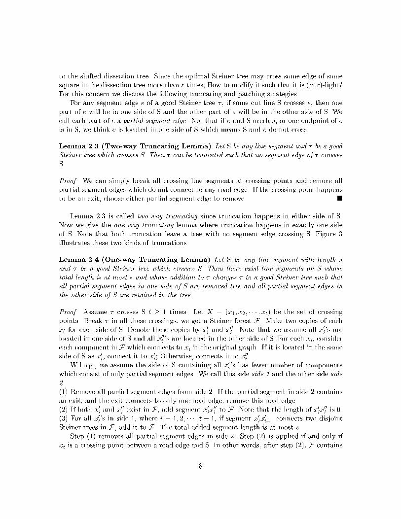
to the shifted dissection tree. Since the optimal Steiner tree may cross some edge of somesquare in the dissection tree more than r times, How to modify it such that it is (m,r)-light?For this concern we discuss the following truncating and patching strategies.For any segment edge e of a good Steiner tree � , if some cut line S crosses e, then onepart of e will be in one side of S and the other part of e will be in the other side of S. Wecall each part of e a partial segment edge. Not that if e and S overlap, or one endpoint of eis in S, we think e is located in one side of S which means S and e do not cross.Lemma 2.3 (Two-way Truncating Lemma) Let S be any line segment and � be a goodSteiner tree which crosses S. Then � can be truncated such that no segment edge of � crossesS.Proof. We can simply break all crossing line segments at crossing points and remove allpartial segment edges which do not connect to any road edge. If the crossing point happensto be an exit, choose either partial segment edge to remove. �Lemma 2.3 is called two-way truncating since truncation happens in either side of S.Now we give the one-way truncating lemma where truncation happens in exactly one sideof S. Note that both truncation leave a tree with no segment edge crossing S. Figure 3illustrates these two kinds of truncations.Lemma 2.4 (One-way Truncating Lemma) Let S be any line segment with length sand � be a good Steiner tree which crosses S. Then there exist line segments on S whosetotal length is at most s and whose addition to � changes � to a good Steiner tree such thatall partial segment edges in one side of S are removed tree and all partial segment edges inthe other side of S are retained in the tree.Proof. Assume � crosses S t � 1 times. Let X = (x1; x2; � � � ; xt) be the set of crossingpoints. Break � in all these crossings, we get a Steiner forest F . Make two copies of eachxi for each side of S. Denote these copies by x0i and x00i . Note that we assume all x0i's arelocated in one side of S and all x00i 's are located in the other side of S. For each xi, considereach component in F which connects to xi in the original graph. If it is located in the sameside of S as x0i, connect it to x0i; Otherwise, connects it to x00i .W.l.o.g., we assume the side of S containing all x0i's has fewer number of componentswhich consist of only partial segment edges. We call this side side 1 and the other side side2.(1) Remove all partial segment edges from side 2. If the partial segment in side 2 containsan exit, and the exit connects to only one road edge, remove this road edge.(2) If both x0i and x00i exist in F , add segment x0ix00i to F . Note that the length of x0ix00i is 0.(3) For all x0i's in side 1, where i = 1; 2; � � � ; t � 1, if segment x0ix0i+1 connects two disjointSteiner trees in F , add it to F . The total added segment length is at most s.Step (1) removes all partial segment edges in side 2. Step (2) is applied if and only ifxi is a crossing point between a road edge and S. In other words, after step (2), F contains8

( a )

S

Road Edge

Segment Edge

Steiner Point

Exit

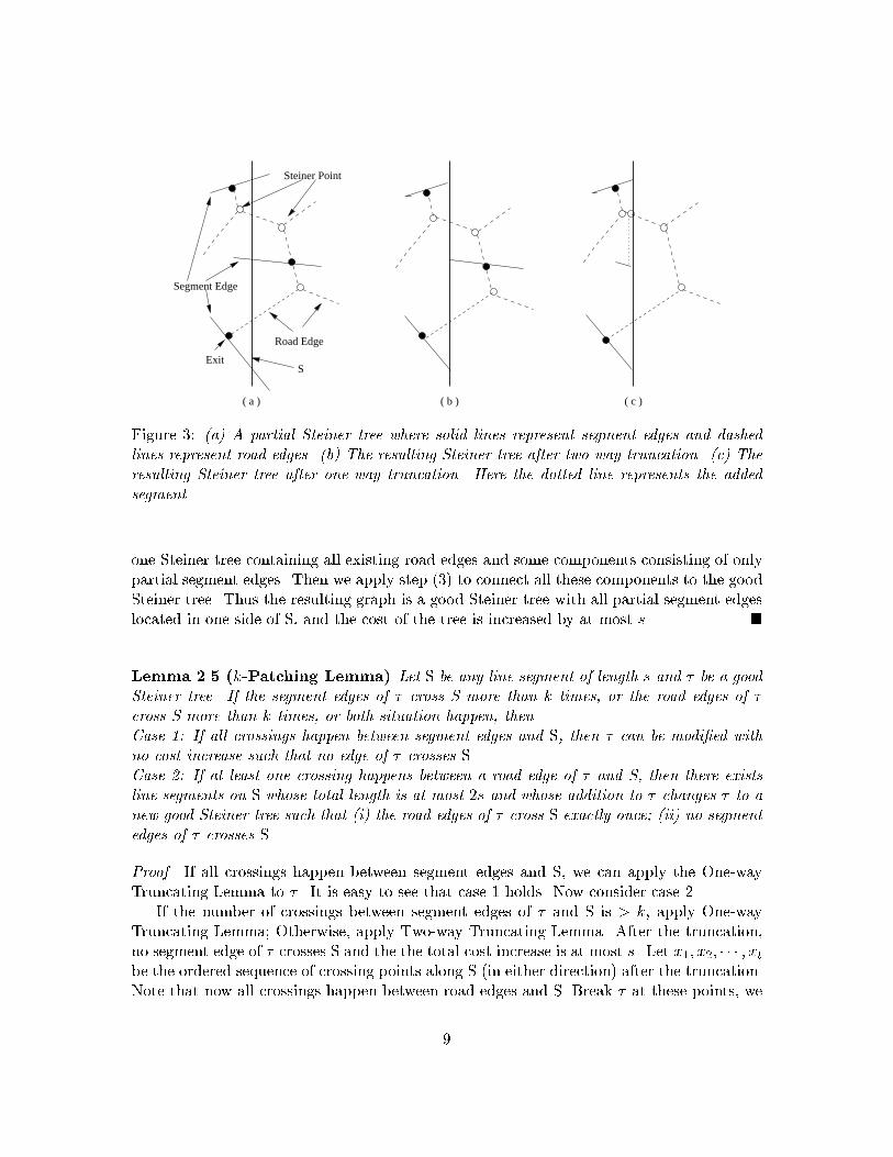
( c )( b )Figure 3: (a) A partial Steiner tree where solid lines represent segment edges and dashedlines represent road edges. (b) The resulting Steiner tree after two-way truncation. (c) Theresulting Steiner tree after one-way truncation. Here the dotted line represents the addedsegment.one Steiner tree containing all existing road edges and some components consisting of onlypartial segment edges. Then we apply step (3) to connect all these components to the goodSteiner tree. Thus the resulting graph is a good Steiner tree with all partial segment edgeslocated in one side of S, and the cost of the tree is increased by at most s. �Lemma 2.5 (k-Patching Lemma) Let S be any line segment of length s and � be a goodSteiner tree. If the segment edges of � cross S more than k times, or the road edges of �cross S more than k times, or both situation happen, thenCase 1: If all crossings happen between segment edges and S, then � can be modi�ed withno cost increase such that no edge of � crosses S.Case 2: If at least one crossing happens between a road edge of � and S, then there existsline segments on S whose total length is at most 2s and whose addition to � changes � to anew good Steiner tree such that (i) the road edges of � cross S exactly once; (ii) no segmentedges of � crosses S.Proof. If all crossings happen between segment edges and S, we can apply the One-wayTruncating Lemma to � . It is easy to see that case 1 holds. Now consider case 2.If the number of crossings between segment edges of � and S is > k, apply One-wayTruncating Lemma; Otherwise, apply Two-way Truncating Lemma. After the truncation,no segment edge of � crosses S and the the total cost increase is at most s. Let x1; x2; � � � ; xtbe the ordered sequence of crossing points along S (in either direction) after the truncation.Note that now all crossings happen between road edges and S. Break � at these points, we9

get a Steiner forest F . Make two copies of each xi, one for each side of S. Denote thesecopies by x0i and x00i . For all i = 1; 2; � � � ; t, let all x0i be located in one side of S, while all x00ibe located in the other side of S.Initially let J be an empty set of line segments. For i = 1; 2; � � � ; t� 1, if segment x0ix0i+1(or x00i x00i+1) connects two Steiner trees in F , add x0ix0i+1 (or x00i x00i+1) to J. Finally add x0tx00tto J. We claim that x0ix0i+1 and x00i x00i+1 can't connect to two disjoint components in F at thesame time since xi and xi+1 break � into only 3 disjoint connected components and these3 components must be located in both sides of S. Thus the total length of all segments inJ is at most s since the length of x0tx00t is 0.Add J to F , the resulting Steiner tree has length at most 2s more than that of theoriginal Steiner tree and it crosses S exactly once. Case 2 holds. �Remarks: (i) Patching Lemma respects the validity of the good Steiner tree. In otherwords, after patching, each segment still has exactly one point (may not be the originalone) connecting to the network. (ii) Patching Lemma tells us that if a Steiner tree crossesan edge of a square in the dissection too many times, we can modify the tree such that itcrosses the edge at most once. The addition of line segments lying on the edge introduces\bent" edges to the Steiner tree.Lemma 2.6 Let � be a Steiner tree with cost T whose edge length is at least 4 units. For agrid line l in the unit grid which covers the tree, let t(�; l) be the number of times � crossesl. Then Xl: vertical t(�; l) + Xl:horizontal t(�; l) � 2 � TProof. Let e be any edge with length s in � . Let a and b be the lengths of the horizontaland vertical projections of e. Then e crosses the grid lines at most a+ b+2 times. We havea+ b � p2 s since a2+ b2 = s2, ab � s22 and a+ b = ps2 + 2 a b. When s � 4, p2 s+2 � 2 swhich means a+ b+ 2 � 2 s. �Remark: Lemma (2.6) relates the length of a Steiner tree to the number of times the treecrosses the grid lines of a unit grid.The proof of the Structure Theorem uses Markov's inequality. We state it as below.Markov's inequality: If X is a random variable in [0;+1) with the mean �, then forany positive constant a, Pr(X � a) � �a .Now we are ready for the proof of Structure Theorem.Proof of Structure Theorem. Let s = 10c, r = s+2, m � 2 s log L. Let � be an optimalSteiner tree which connects all given line segments in a perturbed instance. Suppose shift(a; b) is picked randomly. We will �rst introduce the concept of level for dissection lines,then transform � into a good Steiner tree which is (m,r)-light with respect to the randomly-shifted dissection. We will charge the cost increase due to transformation to each unit gridline. Note that we assume L is a power of 2. Then the vertical lines and horizontal lines10

in the dissection lie in the unit grid lines. From now on, we use grid lines to refer to bothdissection lines and unit grid lines.Recall that the dissection is the recursive partition of the bounding square. And weview a dissection as a hierarchical 4-ary dissection tree. Each node in the dissection tree isone square, and all squares in the same level have equal size. So naturally each square hasa level. The root square has level 0. It's 4 child squares have level 1. . . . All leaf squareshave level log L. Since the side of each square is part of some vertical or horizontal lines,we introduce a level for each grid line accordingly.In a dissection with shift (a; b), the leftmost vertical line is in x-coordinate a and thelowest horizontal line is in y-coordinate b. These two grid lines have level 0 since theycontribute to the level 0 square in the dissection tree; The vertical lines (x = a, x =L2 + a mod L) and the horizontal lines (y = b, y = L2 + b mod L) have level 1 since theycontribute to level 1 squares; Generally speaking, the vertical lines (x = a+p � L2i mod L) forp = 0; 1; � � � ; 2i � 1, and horizontal lines (y = b+ p � L2i mod L) for p = 0; 1; � � � ; 2i � 1, havelevel i, where i = 0; i; � � � ; log L, since they contribute to level i squares in the dissectiontree. It is clear that a level i grid line is also a level i + 1; � � � ; log L grid line. The highestlevel of a grid line is the highest level among all squares it contributes.Since the shift (a; b) is picked randomly, for each vertical grid line l and each 1 � i �log L, Pr[l is at level i] = 2iL (1)Pr[the highest level of l is i] = 2i�1L (2)(Because totally there are L vertical lines, 2i of them are at level i and 2i�1 of them havehighest level i.) Similar arguments hold for horizontal lines.Now we want to modify the optimal Steiner tree � into a good Steiner tree which is (m,r)-light. We �rst make � (m,s)-light. Then we explain why we need the 2 extra crossings oneach square edge in the shifted dissection tree.The modi�cation will be done in a topdown fashion with respect to the dissection treewith random shift (a; b). At level i, there are 4i squares. We will �rst make both road edgesand segment edges of � cross each edge of each level i square at most s times; Then weforce the crossings with road edges of � happen at portals. When all levels are visited, weget a (m,r)-light Steiner tree. We will use probability method (over random shift (a; b)) toanalyze this procedure.How to modify � such that both road edges and segment edges cross each edge of eachlevel i square at most s times? the relationship between grid lines with highest level i andlevel i squares suggests the following way: Go through all grid lines. If a grid line l hashighest level i, then go through each of its 2i segments of length L2i and applying s-PatchingLemma whenever one of them is crossed by the road edges or segment edges of the currentgood Steiner tree more than s times. But we can not apply Patching Lemma directly tothe segment with > s crossings because we may introduce too much cost increase. Since lis also at level i+ 1; � � � ; log L, a better idea is to apply Patching Lemma bottom up for all11

i � j � log L. The following procedure MODIFY(l; i; a) does the patching for vertical line lwhose highest level is i in a dissection with random horizontal shift a.MODIFY(l; i; a)For j = log L down to i doFor p = 0; 1; � � � ; 2j�1, if the segment of l between they-coordinates (a+p � L2j mod L) and (a+ (p+ 1) � L2j mod L)is crossed by the road edges or segment edges ofthe current good Steiner tree more than s times,then apply s-Patching Lemma to reduce the numberof crossings to 2.Remarks on MODIFY: (i) Patching Lemma reduces the number of crossings to 2 instead of1 because we must do patching separately for the 2 parts of a \wrapped around" square.(ii) The modi�cations are done in the \bottom-up" fashion. When we consider squares inlevel i + 1; � � � ; log L in the dissection tree, we do not need to check l again even though lcontributes to some squares in level i+1; � � � ; log L. In other words, all charges to grid linel whose highest level is i are due to the level i modi�cation. (iii) The patching increasesthe cost of the current good Steiner tree. It may also increase the number of times thegood Steiner tree crosses a horizontal line h. If the patching along l increases the numberof crossings of the tree with h at least twice, we can apply 1-Patching Lemma to thesecrossings and reduce the number to 2 (do patching for each side of l). This patching doesnot increase cost since all crossings happen in the cross point of l and h. That's the reasonwhy we choose r = s+2 to make the good Steiner tree (m,r)-light. (iv) A similar procedureand arguments hold for horizontal lines with shift b.Let cl;j(a) be the number of segments to which we do patching for each j in MODIFY(l; i; b).Note that cl;j(a) is independent of i since the loop computation for j does not depend on iin MODIFY. Thus Xj�1 cl;j(a) � t(�; l)s� 1 (3)where t(�; l) denote the number of times the good Steiner tree � crosses grid line l. Theinequality holds because each application of Patching Lemma counted on the lefthand sidereplaces at least s + 1 crossings by at most 2. Thus the cost increase due to patching inMODIFY is: �costpatching(l; i; a) �Xj�i cl;j(a) � 2L2j (4)where the term 2L2j comes from Patching Lemma. We charge this cost to l. Of course onlywhen the highest level of l is i do we charge l the cost increase due to patching.Similar analysis holds true for level i horizontal lines.Now in the current good Steiner tree both road edges and segment edges cross each edgeof each level i square in the shifted dissection tree at most m times. We need to move each12

crossing point with road edges to its nearest portal. We call this procedure relocation. Notethat crossing points with segment edges do not relocate.If a line l is at level i, each of the t(�; l) crossings might have to be displaced by L2i+1m toreach its nearest portal. Instead of actually de ecting the edge, we break it at the crossingpoint and add two line segments (one on each side of l) of total length at most L2i m suchthat the new edge crosses l at a portal. Thus we have�costrelocation(l; i; a) � t(�; l) � L2im (5)From the above analysis, we know that the total cost increase charged to a level i verticalline l is: �costtotal(l; i; a) � t(�; l) � L2im +Xj�i cl;j(a) � 2L2j (6)while to a level i horizontal line l is:�costtotal(l; i; b) � t(�; l) � L2im +Xj�i cl;j(b) � 2L2j (7)Consider all vertical grid lines. With probability 2i�1L over random shift (a; b) (see (2)),a vertical grid line has highest level i. According to the Linearity of Expectations, theexpected cost increase charged to a vertical grid line l is:Ea[cost(l; i; a)] � Plog Li=1 2i�1L � ht(�; l) � L2i m +Pj�i cl;j(a) � 2L2j i= log L2m � t(�; l) +Plog Li=1 2iPj�i 12j � cl;j(a)= log L2m � t(�; l) +Plog Lj=1 cl;j(a)2j Pji=1 2i� log L2m � t(�; l) + 2 �Plog Lj=1 cl;j(a)� log L2m � t(�; l) + 2 t(�;l)s�1� 5 t(�;l)2 s (8)where the last inequality holds when s � 9 and m � 2 s log L. Similarly for any horizontalline l, and horizontal shift b, we haveEb[cost(l; i; b)] � 5 t(�; l)2 s (9)From Lemma 2.6 and again Linearity of Expectations, the expected total cost increasedue to modi�cation is: Xl: vertical 5 t(�; l)2 s + Xl: horizontal 5 t(�; l)2 s � 5OPTs (10)Since s = 10c, the expected cost increase is at most OPT2 c . According to Markov's In-equality, with probability at least 12 the cost increase is no more than OPTc . �13

2.4 The AlgorithmStructure Theorem tells us that with probability at least 12 , There exists a (m,r)-light Steinertree with cost at most (1 + 1c )OPT . This suggests the following algorithm:Step 1. Perturb and rescale the given instance.Step 2. Construct a quadtree with random shift (a; b) based on the perturbedinstance.Step 3. Find an optimal (m,r)-light Steiner tree with respect to the dissectionwith shift (a; b) by dynamic programming.We have explained step 1 and 2 in detail in previous sections. Now we focus on thedynamic programming procedure.The basic idea comes from the following observation. Suppose S is a square in the shiftedquadtree and the optimal (m,r)-light Steiner tree crosses the boundary of S a total of � 4 rtimes. Not that all the crossings with road edges happen at portals.The part of the optimal (m,r)-light Steiner tree residing inside S forms a Steiner forest ofp trees with the following characteristics: (i) each of the p trees connects some line segmentsand some portals of S. (ii) all p trees together connect all line segments completely inside Sand a subset of line segments which cross S. (iii) the collection of these p trees is (m,r)-light.That is, they collectively cross each edge of each square in the subtree rooted at S at mostr times, and the crossings with road edges always happen at portals.Since the (m,r)-light Steiner tree is optimal, each of the p trees must be optimal. Thismotivates us to de�ne the following (m,r)-light Steiner forest problem. An instance of the(m,r)-light Steiner forest problem is speci�ed by(a) A square S in the shifted quadtree.(b) A multiset B containing � r portals on each of the four sides of S.(c) A partition of B into (B1; B2; � � � ; Bp).(d) A subset M containing � 4r line segments which cross S. The number of crossingson each of the four sides of S is � r.Note that if one edge (denoted by s1) of S crosses more than m line segments, we breakall these line segments at the crossings and choose to let S include all these segments byremoving all partial line segments out of S, or to totally omit all these line segments byremoving all partial line segments inside S. In the �rst case, all these crossing line segmentsare completely inside S. In the second case, none of them is inside S. In both cases, Mcontains none of these line segments. If the number of crossings is � m, we choose a subset(with cardinality� r) of these line segments and include the subset in M. If one line segmentcrosses two edges of S, the decision must respect the singularity of the line segment, thatis, either S contains the line segment, or S does not contain it at all.We are going to �nd an optimal (m,r)-light collection of p Steiner trees with the ithtree contains all portals in Bi and all trees together connect all line segments which are14

completely inside S and all line segments in M which cross S. Note that the crossing pointswith line segments in M are located in S. Each instance in S can be broken into manysmaller and simpler instances of (m,r)-light Steiner forest problem in the 4 child squares ofS. Instances corresponding to the leaf nodes of the quadtree are solved in a brute-force way.We build a lookup table in a bottom-up fashion for dynamic programming. The numberof entries in the table equals ](a) � ](b)� ](c)� ](d)where ](x) is the number of choices for (x).We already know that ](a) = O(n2 log (n)). With a simple combinatorial analysis, wehave ](b) = O(24m+4r), ](c) = O(2O(4r)) (no edge crossings), and ](d) = O(24m). Thus thetotal number of entries in the lookup table is O(n2 log (n) � 28m+O(4r)). When m = O( log nc ),this number becomes O(nO(c)log(n)).If an entry corresponds to an instance in a leaf node of the quadtree, since there are atmost O(r) portals and at most one line segment, we can solve it by brute-force which takesO(2O(r)) time. If an entry corresponds to an instance in the root node of the quadtree, noportals will be chosen for multiset B and no crossing line segments will be chosen for Msince the root node contains all line segments. The result is an (m,r)-light Steiner tree andis the output of the dynamic programming. For all other entries, we need to compute the(m,r)-light Steiner forest inductively. Let S be any nonleaf square in the quadtree and letS1, S2, S3, S4 be its four children. Each choice of (b), (c), (d) for S decides an instanceI. To compute the entry for I, we must consider all possible ways in which an (m,r)-lightSteiner tree could cross the edges of S1, S2, S3, S4. This means we need to enumerate alltriples of the following kind:(a') A multiset B' containing � r portals in each of the 4 inner edges of the child squares.(The outer edges of the 4 children are part of the edges of S. So, the number of portals, thepartition of these portals, and the crossing line segments are all set.)(b') A partition of B' into (B1; B2; � � � ; B0p0).(c') A subset M0i for each of the 4 child squares containing � r line segments crossingeach of the two inner edges of the child square, where i = 1; 2; 3; 4.When we choose M0i for each child square, we must consider the following situationssince each inner edge contributes to two squares. Let's use squares S1 and S2 which sharethe common inner edge e as an example. If the number of line segments crossing e is > m,We have only two choices. We either let S1 contains all of these line segments by removingall partial segments out of S1, or let S2 contains all of these line segments by removing allpartial segments out of S2. In both cases, M01 and M02 contain none of these line segments.If the number of line segments crossing e is � m, for each of these line segments, we chooseto let either M01 or M02 contains this segment.Note that each choice of (a'), (b') and (c') decides a smaller instance for each of the 4 childsquares. Since the optimal (m,r)-light Steiner forest to all instances in the 4 child squaresare already in the lookup table (by induction), we do not need to compute them again.We union the 4 (m,r)-light Steiner forests to get an (m,r)-light Steiner forest for instance I15

but this Steiner forest may not be optimal. Each choice of (a'), (b') and (c') results in an(m,r)-light Steiner forest for I and the one with smallest cost is the one that will be put intothe table for instance I. Since ](a0) = O(24m+4r), ](b0) = O((4r)! 2O(4r))(no edge crossings)and ](c0) = O(24m) the running time for each entry takes O((4r)! � 28m+O(4r)) = O(nO(c))when m = O( log(n)c ) and r = O(c).For those \wrapped-around" squares, we treat them as normal squares, except that theyare already divided into 2 or 4 rectangles. The choices of (b), (c) and (d) and the choicesof the corresponding (a'), (b') and (c') must respect these divisions.Remarks on dynamic programming: (i) The dynamic programming procedure de-scribed above computes only the cost of the optimal (m,r)-light Steiner tree. We canconstruct the (m,r)-light Steiner tree by looking at the decisions made for each step of thedynamic programming. (ii) As mentioned earlier, We can run dynamic programming for allchoices of random numbers a and b, and choose the output with smallest cost for the giveninstance. This increase the running time by a factor O(n2). (iii) In the induction analysisof dynamic programming for instance I, the portals in the 4 edges of S may not overlapwith portals in the outer edges of the 4 children of S. Thus we can not union the optimalsolutions to the 4 children to get a (m,r)-light Steiner forest for I. This problem can beavoided by forcing m to be a power of 2. (iv) Steiner nodes may be introduced when wecompute the (m,r)-light Steiner forest for each leaf node of the quadtree.3 Conclusion and DiscussionIn this paper we study the problem of Interconnecting Highways. This is the generalizedminimum Steiner Tree problem where the terminals are located in some line segments. Wenot only need to \guess" the locations of Steiner points, but also need to locate the terminalpositions, called exits, in each line segment. We present a PTAS for this problem.Some similar problems arise in these years. For example, given n �xed nonempty convexpolytopes in the Euclidean d-space Rd, �nd a shortest network to connect all these polytopeswith the constraints that each polytope has exactly one point to be connected to the network[14]. Another example, given a set of local networks, construct a global network to connectall the local networks. The global network must form a connected network of its own [11].These two problems can be treated as the generalized Interconnecting Highways problem.And polynomial time approximation schemes may exist by including some parameters inthe objective functions and applying similar idea.References[1] S. Arora, Polynomial Time Approximation Schemes for Euclidean Traveling Salesmanand other Geometric Problems, Proceedings of 37th IEEE Symposium on Foundationsof Computer Science, (1996) 12 16

[2] S. Arora, Polynomial Time Approximation Schemes for Euclidean TSP and other Ge-ometric Problems, (1997). Available from http:www.cs.princeton.edu/�arora[3] M. Bern, D. Eppstein and S.-H. Teng, Parallel Construction of Quadtree and QualityTriangulation, Proc. 3rd WADS, Springer Verlag LNCS 709, (1993) 188-199[4] G.X. Chen, The shortest path between two points with a (linear) constraint, Knowledgeand Appl. of Math., 4 (1980) 1-8[5] D.-Z. Du, F.K. Hwang, A Proof of Gilbert-Pollak's conjecture on the Steiner ratio,Algorithmica, 7 (1992) 121-135[6] D.-Z. Du, F.K. Hwang, and G.L. Xue, Interconnecting Highways, SIAM Discrete Math-ematics, 12 (1999) 252-261[7] D.-Z. Du, B. Lu, H. Ngo and P.M. Pardalos, Steiner Tree Problems, manuscript (2000)[8] M.R. Garey, R.L. Graham and D.S. Johnson, The complexity of computing Steinerminimal trees, SIAM J. Appl. Math., 32 (1977) 835-859[9] D.S. Hochbaum and W. Maass, Approximation Schemes for Covering and PackingProblems in Image Processing and VLSI, J. ACM, 32 (1985) 130-136[10] F.K. Hwang, D.S. Richards and P. Winter, The Steiner Tree Problem, Annals of Dis-crete Mathematics, North-Holland, (1992)[11] E. Ihler, G. Reich and P. Widmayer, On Shortest Networks for Classes of Points in thePlane, LNCS 553 (1991) 103-111[12] T. Jiang and L. Wang, An Approximation Scheme for some Steiner Tree Problems inthe Plane, LNCS 834 (1994) 414-422[13] J.F. Weng, Generalized Steiner Problem and Hexagonal Coordinate (in Chinese), ActaMath. Appl. Sinica, 8 (1985), 383-397[14] G.L. Xue, D.-Z. Du, and F.K. Hwang, Faster Algorithm for Shortest Network underGiven Topology, manuscript

17