DI

SC

US

SI

ON

P

AP

ER

S

ER

IE

S

Forschungsinstitut zur Zukunft der ArbeitInstitute for the Study of Labor

Team Structure and the Effectiveness ofCollective Performance Pay

IZA DP No. 6747

July 2012

Marisa RattoEmma TomineyThibaud Vergé

Team Structure and the Effectiveness

of Collective Performance Pay

Marisa Ratto Université Paris-Dauphine (Leda-SDFi)

Emma Tominey

University of York and IZA

Thibaud Vergé

CREST, LEI

Discussion Paper No. 6747 July 2012

IZA

P.O. Box 7240 53072 Bonn

Germany

Phone: +49-228-3894-0 Fax: +49-228-3894-180

E-mail: iza@iza.org

Any opinions expressed here are those of the author(s) and not those of IZA. Research published in this series may include views on policy, but the institute itself takes no institutional policy positions. The Institute for the Study of Labor (IZA) in Bonn is a local and virtual international research center and a place of communication between science, politics and business. IZA is an independent nonprofit organization supported by Deutsche Post Foundation. The center is associated with the University of Bonn and offers a stimulating research environment through its international network, workshops and conferences, data service, project support, research visits and doctoral program. IZA engages in (i) original and internationally competitive research in all fields of labor economics, (ii) development of policy concepts, and (iii) dissemination of research results and concepts to the interested public. IZA Discussion Papers often represent preliminary work and are circulated to encourage discussion. Citation of such a paper should account for its provisional character. A revised version may be available directly from the author.

IZA Discussion Paper No. 6747 July 2012

ABSTRACT

Team Structure and the Effectiveness of Collective Performance Pay

The adoption of performance related pay schemes has become increasingly popular in the public sector of several countries. In the UK, the scheme designers favoured collective performance pay with the aim to foster cooperation across offices. The resulting team structure included several offices (subteams) within the same team, defined by the remuneration scheme. In this paper we analyse the strategic interactions across subteams created by a two-level team structure, in order to assess whether rewarding collective performance necessarily promotes cooperation. We show that such team structure creates conflicting incentives to free-ride across and within subteams. Moreover, the relative size of subteams can be a powerful means to deliver incentives when funds for performance rewards are limited. Using data for one of the incentive schemes piloted in the UK, we analyse the role of the target level and of the relative size of subteams on subteams’ performance. JEL Classification: M52, M54, J33 Keywords: incentives, teams performance, sub-teams, cooperation Corresponding author: Emma Tominey Department of Economics The University of York Heslington, York. YO10 5DD United Kingdom E-mail: emma.tominey@york.ac.uk

1 Introduction

The use of performance related pay (PRP) has become very popular in the civil service of

several countries. It is estimated that two-thirds of OECD member countries have imple-

mented PRP or are in the process of doing so (OECD, 2004a). Over the past few years

one of the common trends emerging across the OECD countries has been the ”...increase

in the use of collective or group performance schemes, at team/unit or organisational

level.”1. The rationale behind the adoption of group performance incentive schemes relies

on the limitations of individual PRP schemes, for example with regard to measuring in-

dividual performance, which is particularly difficult in the public sector. Public services

are typically delivered through complex organisations, consisting of multiple divisions and

a widespread network of offices. In these contexts, output, even when it is quantifiable,

may be very costly to measure at individual level, as sophisticated data management

systems are required. As a result, only aggregate measures may be available. The United

Kingdom is one of the countries who have strongly encouraged the move towards a more

collective approach to PRP. A number of departments have been piloting team-based

schemes since 2001, following the recommendations of the Makinson report (Makinson,

2000). A common feature of these trial schemes is the definition of a team on the basis of

administrative considerations. In particular, teams have been created by the reward sys-

tem, at the level of a division, comprising different offices, although there are no apparent

operational links within those offices. Informal discussions with some of the designers of

these schemes revealed that one of their main concerns was to create collaboration across

offices, which, for this reason, were included in the same team.

This paper addresses some important issues arising from such an incentive scheme

design. Setting targets and assessing performance at the level of a division creates in-

terdependencies among the offices in the same division. In fact, the expected reward of

an office for hitting the target depends on how far actual performance at division level is

from the target. This is determined by all offices’ output. However, production occurs at

the level of offices, where complementarities in production may be at work (final output

may depend on the effort of different colleagues)2. Hence the structure of the team is

quite complex, and results in a two-level team: ”natural” teams or subteams (offices)

are included within ”reward” teams (divisions). Both the theoretical and empirical liter-

ature focus on teams defined by the production process, by the nature of the activities

performed or by some common interest or motivation that may drive teamwork. In Holm-

strom’s (1982) seminal paper a team is either defined by the production process, or on

the basis of some common uncertainty which affects the measurement of individual out-

1See OECD, 2004b, p. 6.2The office would be a team à la Holmström (1982), identified by complementarities in production.

2

puts. The individual choice of effort in teams is also analysed in contexts where teamwork

emerges as the result of implicit incentives, such as peer pressure (Kandel-Lazear (1992)

and Encinosa et al (1997)), or long-term repeated interactions among workers (Che and

Yoo, 2001), or intrinsic motivation, when cooperation among workers spontaneously arise

because workers care about the output of the organisation (Francois, 2000). The nature of

tasks and individual preferences towards tasks may also motivate the optimal adoption of

teamwork (Itoh, 1991). In these settings teams are endogenous, identified by the implicit

incentives that might be at work in the different contexts. In this paper we consider teams

like the ones defined in the pilot schemes introduced in the UK government agencies, i.e.

exogenously created by an externally imposed reward scheme. Given the recent adoption

of similar incentive schemes in the OECD member countries, the analysis provides, to

our knowledge, a novel contribution which can supply testable predictions and inform the

design of incentives mechanisms in the public sector.

We address two main issues arising from incentive schemes in two-level teams. We

examine i) what kind of interdependencies in effort choice can be triggered across subteams

when these are rewarded on the basis of their aggregate output (team output), and ii)

how does the relative size of subteams affect the team’s output for different levels of the

bonus. In particular, we consider a situation where resources to be used for the award of

the bonus are limited and hence the principal cannot set the first-best level of the bonus.

Results show that the design of the scheme has important implications not only on

the level of effort chosen by single subteams, but also on the nature of subteams’ inter-

dependencies. In particular, the reaction function of each subteam differs for different

target levels. Whether subteams’ efforts are positively or negatively related or completely

independent depends on the magnitude of the target, as this affects the probability of suc-

cess and hence the expected marginal benefit of effort of the subteam. Hence cooperation

across subteams is not automatically created by rewarding subteams on the basis of their

aggregate output. One implication of our results is that the relative size of subteams can

be a powerful means to deliver incentives: instead of increasing the bonus the principal

can alter the relative size of subteams to foster positive interdependencies in subteams’

effort. This alternative incentive tool may be particularly valuable in the presence of

budgetary constraints in the allocation of bonuses, when the principal cannot increase

financial rewards to improve outcomes as optimally required. If the bonus has to be set

at a low level, there is a unique value of asymmetry in subteams’ size that allows the

principal to get the highest level of output (second-best). If the principal can set a high

bonus, then the first-best can be achieved with perfect symmetry. This suggests that the

size of subteams shouldn’t be taken as given by the scheme designers, but should be a

strategic variable like the targets and the bonus.

We organise the paper as follows. In the next section we discuss the design of three

3

incentive schemes, piloted in the UK government between April 2001 and March 2003.

Section 3 presents a simple ad-hoc model that captures the two-level team structure of the

incentive mechanisms discussed in section 2. In section 4, the best response of the subteam

(office) is derived. The principal’s optimal choice of the incentive parameters is analysed

in section 5. Section 6 considers the subteams’ relative size as a strategic variable for a

principal with limited resources to reward performance. In section 7 we test the impact

of the target level and of the asymmetry in subteams’ size on team’s performance, using

data from one of the public agencies’ schemes mentioned above. Results are summarised

in the conclusion.

2 The introduction of team-based incentives in the

UK public sector: characteristics of the schemes

The incentive schemes we present in this section were part of a programme to reform

public service delivery, started in the UK in 1997 and aimed at improving efficiency and

productivity of the public sector. The idea of piloting a team-based incentive scheme in

public agencies dates back to the Makinson report (2000). John Makinson (then Group

Finance Director of Pearson plc) was recruited to the Public Service Productivity Panel to

analyse how performance-based incentives operated in four public organisations (Benefits

Agency, Employment Service, HM Custom and Excise, and Inland Revenue) and how

they might be improved. In his report particular emphasis was placed on the use of

team-based incentives, with the view that teamwork better reflects the way in which most

public servants actually work. Most of the recommendations of the report were taken on

board by the scheme designers of three governmental agencies: Child Support Agency,

Jobcentre Plus and HM Customs and Excise3. In Particular, incentives related to targets

already embodied in the Public Service agreements (PSA)4 of the respective agencies, as

we shall consider below. There were up to five targets and if these were reached extra

bonuses would be paid, separated out from basic pay and not consolidated into salaries.

Teams were defined within the administrative boundaries of a division/district, comprising

different offices in different locations.

In Child Support Agency the scheme ran from April 2001 to end of March 2002. Teams

were defined at Business Unit (BU) level, in that the targets were defined at BU level and

all workers within the BU received the bonus if the target was hit, regardless of individual

performance. These teams were very big; there were only six BUs covering the whole

3For a quantitative evaluation of these schemes see Burgess et al. (2004, 2005, 2008).4These are performance indicators introduced in 1998 by the Comprehensive Spending Review (CSR),

to drive improvements in outcomes in the public sector.

4

of the country, varying in size from 10 to 24 offices in the team and 1350 to 1650 staff

in the team. There were three sets of targets, assessed on a quarterly basis. Each of

the three sets of targets accrued 0.5 of salary bonus for each quarterly checkpoints, with

a maximum achievable bonus of 5% of salary. In common with the other two agencies,

the bonus was paid for hitting the target, but no further increase for additional output

was available. Thus incentives were very sharp at output levels just below the target

threshold, but weaker further below and flat for output levels above the threshold.

The scheme for HM Customs and Excise was implemented in six trial sites and ran

for nine months from April 2002 through December 2002. The unit chosen by HMCE

as the team was a Division, which typically comprised a small number of offices5. The

teams had five targets to reach. These were a subset of the annual PSA targets setting

a baseline level of performance and to which a stretch of 5% performance improvement

was applied for incentive purposes. Two different reward schemes were implemented. In

one case the bonus varied according to the individual’s job band. In the other case, the

bonus paid was equal across all team members including the team manager. On average,

the bonus was worth about 3% of salary6.

In Jobcentre Plus the scheme ran from April 2002 to the end of March 2003. The

team unit was the district. Once again, these were big teams - there were only 90 districts

covering the whole of the country, varying in size from 5 to 39 offices in the team, and

from 264 and 1535 people within a team. 17 out of the 90 districts were selected for

the incentive scheme. The incentive targets consisted of the annual PSA Jobcentre Plus

targets, to which a stretch factor was added (5% or 7.5% depending on the district). In

total there were five incentivised targets, each of one carrying a fixed bonus for each team

member, varying according to their grade. The District had to hit at least two targets to

get any bonus, and if all 5 were reached, 50% of the standard rate per grade was paid as

an addition7.

An important characteristic, common across all three schemes, is that outcomes are

produced, measured and assessed at different levels in the hierarchy of the organisations.

This has important implications on the structure of the teams and ultimately on the

effective delivery of incentives. Incentive targets and rewards for achieving those tar-

gets are set at team level. Teams are defined within the administrative boundaries of

a division/district, comprising different offices in different locations. Setting targets and

assessing performance at the level of a division/district creates interdependencies among

5In the pair of trial teams evaluated, there were up to 6 offices and up to 158 staff in the team.6Our conversations with HMCE officials suggested that it was seen by the managers as a worthwhile

amount for the extra effort to achieve the targets.7This meant that if all five targets were hit, the bonus that a worker could gain would vary from £750

to £3,750.

5

the offices in the same division/district. In fact, the expected reward of an office for hit-

ting the target depends on how far actual performance at team level is from the target.

And this is determined by all offices’ output. Production occurs at individual level, or, if

members of staff in an office interact with each other and contribute to the same outcome,

at office level. We were informed that in all three organisations there are no apparent

operational links within offices belonging to the same division/district, so that they do

not contribute to the same outcome.

Hence we have teams created by the reward system at the level of a division/district

whereas output is produced at the level of an office. The structure of the teams is quite

complex, and results in a two-level team: natural teams (offices), which contribute to

a common output, are included within reward teams (divisions/districts). In the next

section we model such a team structure, created by the incentive scheme and analyse the

best response at the level of a subteam (office). We shall address two questions: 1) Is

subteams’ cooperation necessarily encouraged by rewarding team performance? 2) What

implications can be drawn on the optimal incentive scheme?

3 The model

We define a subteam as a natural team, where complementarities in production are

present. We can think of it in terms of an office. A team is, instead, the unit upon

which output is assessed for incentive purposes. Let

qi = f(Ni, ei) + εi (1)

be subteam i’s total output, where Ni is the number of staff in subteam i, ei is the mean

effort level, and εi is an idiosyncratic random shock. The total number of staff in the

team is∑Ni = N .

We define B as the bonus which is payable if the target on performance is achieved. As

in the schemes we presented above, we model the bonus as a fixed amount (for example a

fixed proportion of salary, as in the schemes mentioned above), paid for hitting the target,

but with no further increase for additional output. So the payoff at team level is:

• NB if∑qi ≥ (1 + γ)q

• 0 otherwise

where q =∑qi is last year performance or some minimum standard expected within

the organisation (like the baseline PSA target) and γ is the improvement in performance

aimed to be reached on the top of last year’s or some minimum performance.

6

The expected payoff for office i is:

Vi(ei) = Pr(∑

qi ≥ (1 + γ)q)NiB − C(Ni, ei) (2)

where C(Ni, ei) is the cost of effort for subteam i.

3.1 Basic assumptions

• We consider a simple setting where there are two subteams within a team, of different

size αi, with α1 = α and α2 = (1− α) and α ≥ 1/2.

• The total number of staff in the team is normalised to 1, i.e. N = 1, so that αi is

the relative size of subteam i.

• There are two possible outcomes of the production process: a subteam’s output can

either be successful or fail. It is successful when output reaches a given critical level:

to minimise the parameters of the model we assume that such a level is qi = αi .

A successful outcome depends on the average effort of a subteam and we assume it

occurs with probability p(ei ) = ei . Failure occurs when qi = qi and this happens

with probability (1− p(ei)) = (1− ei).

• The cost of effort is quadratic in effort and subteam size: Ci =c2(αiei)

2

3.2 Office output, target levels and probability of success

We now define output in each subteam and at team level, the targets and the probability

of reaching the target.

• Output

Under the assumption we made on the possible outcomes, or states of the world, there

are four possible ranges of output, at subteam and team level:

Possible outcomes Subteam 1 output Subteam 2 output Aggregate output

e1e2 α (1− α) 1

e1(1− e2) α q2

α+ q2

(1− e1)e2 q1

(1− α) (1− α) + q1

(1− e1)(1− e2) q1

q2

q1+ q

2

In Figure 1 we represent these possible ranges of aggregate output.

• Targets

7

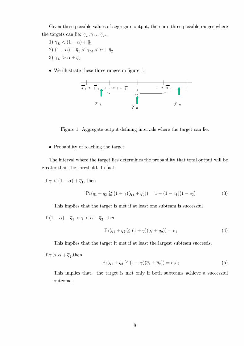
Given these possible values of aggregate output, there are three possible ranges where

the targets can lie: γL, γM , γH .

1) γL < (1− α) + q1

2) (1− α) + q1< γM < α+ q2

3) γH > α+ q2

• We illustrate these three ranges in figure 1.

1

Lγ

21qq +

1)1( q+− α 2

q+α

Mγ Hγ

2

1

Figure 1: Aggregate output defining intervals where the target can lie.

• Probability of reaching the target:

The interval where the target lies determines the probability that total output will be

greater than the threshold. In fact:

If γ < (1− α) + q1, then

Pr(q1 + q2 ≧ (1 + γ)(q1 + q2)) = 1− (1− e1)(1− e2) (3)

This implies that the target is met if at least one subteam is successful

If (1− α) + q1< γ < α+ q

2, then

Pr(q1 + q2 ≧ (1 + γ)(q1 + q2)) = e1 (4)

This implies that the target it met if at least the largest subteam succeeds,

If γ > α+ q2,then

Pr(q1 + q2 ≧ (1 + γ)(q1 + q2)) = e1e2 (5)

This implies that. the target is met only if both subteams achieve a successful

outcome.

8

4 Optimal effort choice at subteam level

In this section we derive the optimal response of a subteam to the incentive mechanism

we introduced in the previous section. Our aim is to analyse whether rewarding aggregate

performance necessarily increases sub-teams cooperation as was the objective of the UK

public sector scheme designers. In order to do this, we need to calculate the reaction

function of each separate sub-unit of the team. Note that we abstract from any free-

riding considerations at the level of the office. Our aim is to examine interactions across

subteams and not within teams. In the schemes we presented in section 2, the district

manager is responsible for the district and devolves the targets to managers in the different

offices. Output is measured at office level. So we can think of an office manager as our

”aggregate unit” of effort decision. Our aim is to examine the impact of the introduction

of team bonuses on offices’ aggregate output.

The expected bonus for each subteam will depend on the probability that the target

at team level is met, and this depends on the magnitude of the target. We can distinguish

threee cases.

Case 1 : γ = γL < (1− α) + q1. Each subteam will solve the following maximisation

problem:

maxei[1− (1− e1)(1− e2)]αiB −

c

2(αiei)

2 (6)

The reaction function for each subteam, derived from the first order condition is:

eRF1

= min

{β(1− e2)

α, 1

}(7)

eRF2

= min

{β(1− e1)

(1− α), 1

}

with β = Bc. In what follows we assume that the cost parameter c is constant across all

teams, so that the value of β = Bc

is determined by the bonus B.

The subteam effort choice is negatively affected by its size and positively by the level

of the bonus, relative to the constant cost parameter. We should point out that here there

is no assumption on complementarity or substitutability of effort between subteams, as

there are no operational links within offices. So any relation between subteams’ effort is

only due to the way the incentive scheme is designed. In this case, when the target is low,

a higher effort by one subteam induces a lower effort by the other subteam, as equation

(7) shows.

The equilibrium levels of effort depend on the magnitude of β relative to α. In par-

ticular, there are three cases:

If the bonus is relatively low, i.e. β < 1 − α < α - the bonus is not enough to even

reward a successful output of the smallest team- there is unique equilibrium. From

9

the reaction functions (7) we get:

e∗1=

β(α− β)

α(1− α)− β2> e∗

2=β(1− α− β)

α(1− α)− β2(8)

The bigger subteam will exert more effort

For intermediate values of the bonus , i.e. if 1 − α < β < α- the bonus is enough to

reward a successful outcome of the smallest team, but not sufficient to reward a

successful outcome of the largest team - there is a unique equilibrium and only the

smaller subteam will exert effort:

e∗1= 0 , e∗

2= 1 (9)

If the bonus is relatively high, i.e. β > α, there are three possible equilibria:

e∗1= 0, e∗

2= 1 (10)

e∗1= 1, e∗

2= 0 (11)

e∗1=

β(β − α)

β2 − α(1− α)< e∗

2=β(1− (1− α))

β2 − α(1− α)(12)

But only (10) and (11) are stable.

We represent these equilibria in Figure 2, first column.

Result 1 If the target is low, such that it is sufficient that only one subteam achieves

a successful outcome in order for the team target to be met, there will be negative strategic

interactions in the subteams’ effort choice. Greater effort by one subteam will induce less

effort by the other subteam.

In this case the aggregate reward system is not enough to enhance cooperation across

subteams, and some form of monitoring will be necessary.

Depending on the level of the bonus, it is possible that the best strategy for the

smallest sub-team - whose contribution to aggregate output (and hence to the likelihood

of meeting the target) is smaller - may be to fully free-ride and exert zero effort. Hence it

is not necessarily the case that sub-teams of smaller size supply greater effort: incentives

to free-ride across sub-teams may conflict with incentive to free-ride within sub-teams,

when the team target is set too low.

Case 2 : (1 − α) + q1< γ = γM < α + q

2.Each subteam will solve the following

maximisation problem:

maxeie1αiB −

c

2(αiei)

2 (13)

10

and the resulting reaction functions are:

eRF1

=β

α(14)

eRF2

= 0

The effort choice of the largest subteam is negatively affected by its size and positively

by the level of the bonus, relative to the constant cost parameter. In this case efforts are

unrelated to each other and the smaller subteam will always choose a zero level of effort.

The equilibrium levels of effort for the larger subteam depends on the bonus:

- if the bonus is relatively low, i.e. β = βL < 1− α < α, or has intermediate values,

i.e. if 1− α < β = βM < α, there is a unique equilibrium:

e∗1=β

α> e∗

2= 0 (15)

- if the bonus is relatively high, i.e. β = βH > α, there is a unique equilibrium:

e∗1= 1 , e∗

2= 0 (16)

We represent these equilibria in Figure 2, second column.

Result 2 If the target can be reached whenever the largest subteam is successful, sub-

teams will choose their effort independently. The smaller subteam will always choose zero

effort and only the larger subteam will exert positive effort. This will be an increasing

function of the bonus and a decreasing function of the relative size of the subteam.

Case 3 : γ = γH > α+q2.Each subteam will solve the following maximisation problem:

maxeie1e2αiB −

c

2(αiei)

2 (17)

and the resulting reaction functions are:

eRF1

= max

{β e2α, 1

}(18)

eRF2

= max

{β e1(1− α)

, 1

}

The effort choice of each subteam depends negatively on α, the size of the subteam and

positively on β = Bc, the value of the bonus relative to the constant parameter of the cost

function. Notice that in this case a higher effort by one subteam induces higher effort by

the other subteam. The equilibrium levels of effort are:

- if the bonus is relatively low, i.e. β = βL < 1− α < α, there is a unique equilibrium

and none of the subteams will exert effort:

e∗1= 0, e∗

2= 0 (19)

11

- for intermediate values of the bonus , i.e. if 1− α < β = βM < α, there two sub-cases:

if β2 < α(1−α) there is a unique equilibrium and none of the subteams will

exert effort:

e∗1= 0 , e∗

2= 0 (20)

if β2 > α(1− α) there are two possible equilibria

e∗1= 0 , e∗

2= 0 (21)

e∗1=β

α, e∗

2= 1 (22)

But only (22) is stable.

- if the bonus is relatively high, i.e. β = βH > α, there are two possible equilibria:

e∗1= 0, e∗

2= 0 (23)

e∗1= 1, e∗

2= 1 (24)

But only (24) is stable.

We represent these equilibria in Figure 2, third column.

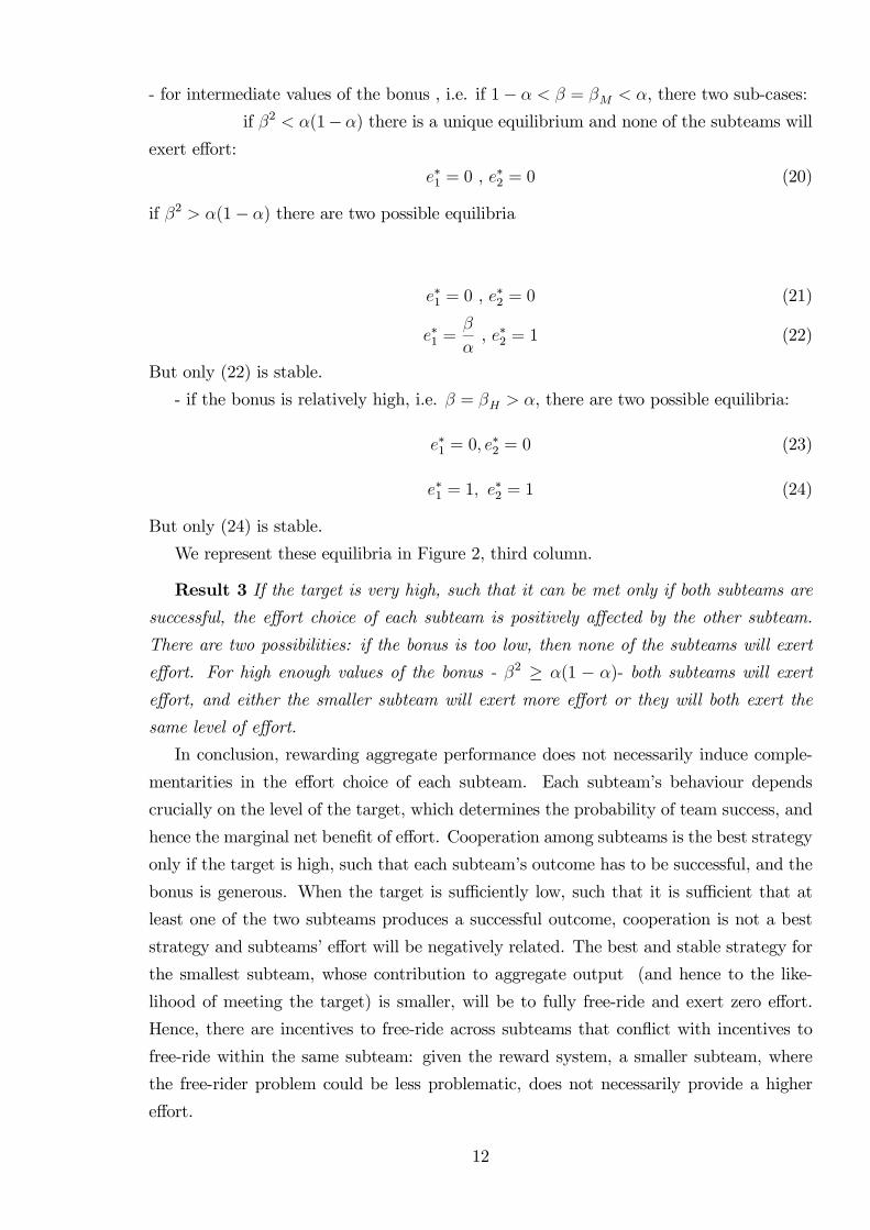
Result 3 If the target is very high, such that it can be met only if both subteams are

successful, the effort choice of each subteam is positively affected by the other subteam.

There are two possibilities: if the bonus is too low, then none of the subteams will exert

effort. For high enough values of the bonus - β2 ≥ α(1 − α)- both subteams will exert

effort, and either the smaller subteam will exert more effort or they will both exert the

same level of effort.

In conclusion, rewarding aggregate performance does not necessarily induce comple-

mentarities in the effort choice of each subteam. Each subteam’s behaviour depends

crucially on the level of the target, which determines the probability of team success, and

hence the marginal net benefit of effort. Cooperation among subteams is the best strategy

only if the target is high, such that each subteam’s outcome has to be successful, and the

bonus is generous. When the target is sufficiently low, such that it is sufficient that at

least one of the two subteams produces a successful outcome, cooperation is not a best

strategy and subteams’ effort will be negatively related. The best and stable strategy for

the smallest subteam, whose contribution to aggregate output (and hence to the like-

lihood of meeting the target) is smaller, will be to fully free-ride and exert zero effort.

Hence, there are incentives to free-ride across subteams that conflict with incentives to

free-ride within the same subteam: given the reward system, a smaller subteam, where

the free-rider problem could be less problematic, does not necessarily provide a higher

effort.

12

βγ

1)1( qL +−< αγ 21)1( qq

M+<<+− αγα

2qH +> αγ

ααβ <−<1L

αβα <<− M1

αβ >H

2221)1(

)1(

)1(

)(

βαα

βαβ

βαα

βαβ

−−

−−=>

−−

−= ∗∗ ee

2

22

)1(

])1([)(

βαα

βααβ

−−

−−+=∗ExpQ

1

0

2

1

=

=

∗

∗

e

e

)1()( α−=∗ExpQ

02

1

=

=

∗

∗

e

eα

β

β=∗)(ExpQ

α−=== 1)( ,1 ,0 )( **2

*11 ExpQeeE

α=== **

2

*

12 )( ,0 ,1 )( ExpQeeE

)1(

])1([)(

)1(

)1((

)1(

)( )(

2

22

*

22213

ααβ

ααββ

ααβ

αββ

ααβ

αββ

−−

−−−=

−−

−−=<

−−

−= ∗∗

ExpQ

eeE

0

1

2

1

=

=∗

∗

e

e

α=∗)(ExpQ

0*

2

*

1 == ee

0)( =∗

ExpQ

0*

2

*

1 == ee

0)( =∗ExpQ)1(2 ααβ −<

)1(2 ααβ −≥

0)( ,0 )( **

2

*

11 === ExpQeeE

αβα

β−+=== 1)( ,1 , )( **

2

*

12ExpQeeE

0)( ,0 )( **

2

*

11=== ExpQeeE

1)( ,1 )(**

2

*

12 === ExpQeeE

)1)(1(1 21 eeprob −−−= 1eprob = 21eeprob =

02

1

=

=

∗

∗

e

eα

β

β=∗)(ExpQ

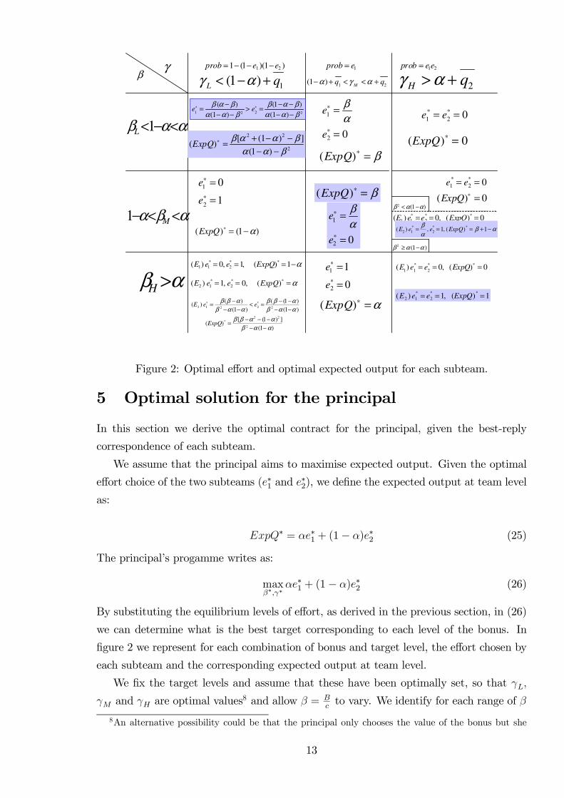
Figure 2: Optimal effort and optimal expected output for each subteam.

5 Optimal solution for the principal

In this section we derive the optimal contract for the principal, given the best-reply

correspondence of each subteam.

We assume that the principal aims to maximise expected output. Given the optimal

effort choice of the two subteams (e∗1

and e∗2), we define the expected output at team level

as:

ExpQ∗ = αe∗1+ (1− α)e∗

2(25)

The principal’s progamme writes as:

maxβ∗,γ∗

αe∗1+ (1− α)e∗

2(26)

By substituting the equilibrium levels of effort, as derived in the previous section, in (26)

we can determine what is the best target corresponding to each level of the bonus. In

figure 2 we represent for each combination of bonus and target level, the effort chosen by

each subteam and the corresponding expected output at team level.

We fix the target levels and assume that these have been optimally set, so that γL,

γM and γH are optimal values8 and allow β = Bc

to vary. We identify for each range of β

8An alternative possibility could be that the principal only chooses the value of the bonus but she

13

whether it is better to set a low, γ = γL, a medium, γ = γM or a high target (γ = γH).

We highlight the optimal solution for the principal in Figure 2. We can distinguish

four different cases:

1) If the bonus is low, i.e. β < 1 − α < α, (first row of the table) then the optimal

target is γ∗ = γL, as this maximises expected output.

2) If the bonus is of intermediate level, i.e. 1− α < β < α (second row in the table)

and β2 < α(1− α), then the optimal target is γ∗ = γM

3) If the bonus is of intermediate level, i.e. 1− α < β < α (second row in the table)

and β2 ≥ α(1− α), then the optimal target is γ∗ = γH

4) If the bonus is high, i.e. β > α (third row) then the optimal target is γ∗ = γH .

If the principal is initially at the top left corner of the table, setting a low target and

low bonus, she is not at a first best. She can be better off at the bottom right corner of the

table, setting a high target and high bonus. In this case, in fact, the expected output is 1,

the maximum attainable. The problem of attaining this equilibrium is that the principal

might have limited resources to use for the bonus payment and hence may not be able to

increase the bonus. An alternative way of reaching the first best is to reduce the degree

of asymmetry in subteams size, α, until β > α.

Result 4 If the principal aims at enhancing cooperation among subteams by use of

aggregate reward systems, the first-best contract requires to set high targets and generous

bonuses. The relative size of subteams is also an important decision variable for the

principal, when bonuses cannot be too generous. In this case, in fact, the principal can

vary the relative size of the subteams to reach a first-best solution.

Hence the composition of a team should not be exogenously determined by some

administrative considerations, but should rather be optimally selected by the scheme

designers, together with the amount of the bonus and the targets. The relative subteams’

size assumes a strategic role, especially when there are monetary constraints on the level

of the bonus to be awarded. We explore this issue more in detail in the next section.

6 Subteams’ relative size as a strategic variable

In this section we consider a situation where the amount of the bonus is fixed and cannot

be chosen. We can either think of a situation where only limited resources can be devoted

to the payment of bonuses, or to a case where the bonuses are exogenously set by a

does not have any choice on the targets and she takes them as given. This would happen when the

targets are optimally set by a body that is different from the designers of the scheme, as it may occur in

organisations like government agencies, where targets are set in concertation with the managers of the

organisation while the funding of the scheme is independently decided by the Treasury.

14

different authority9. We fix β = β < 1

2and examine what is the optimal subteam relative

size, which maximises expected output for the principal.

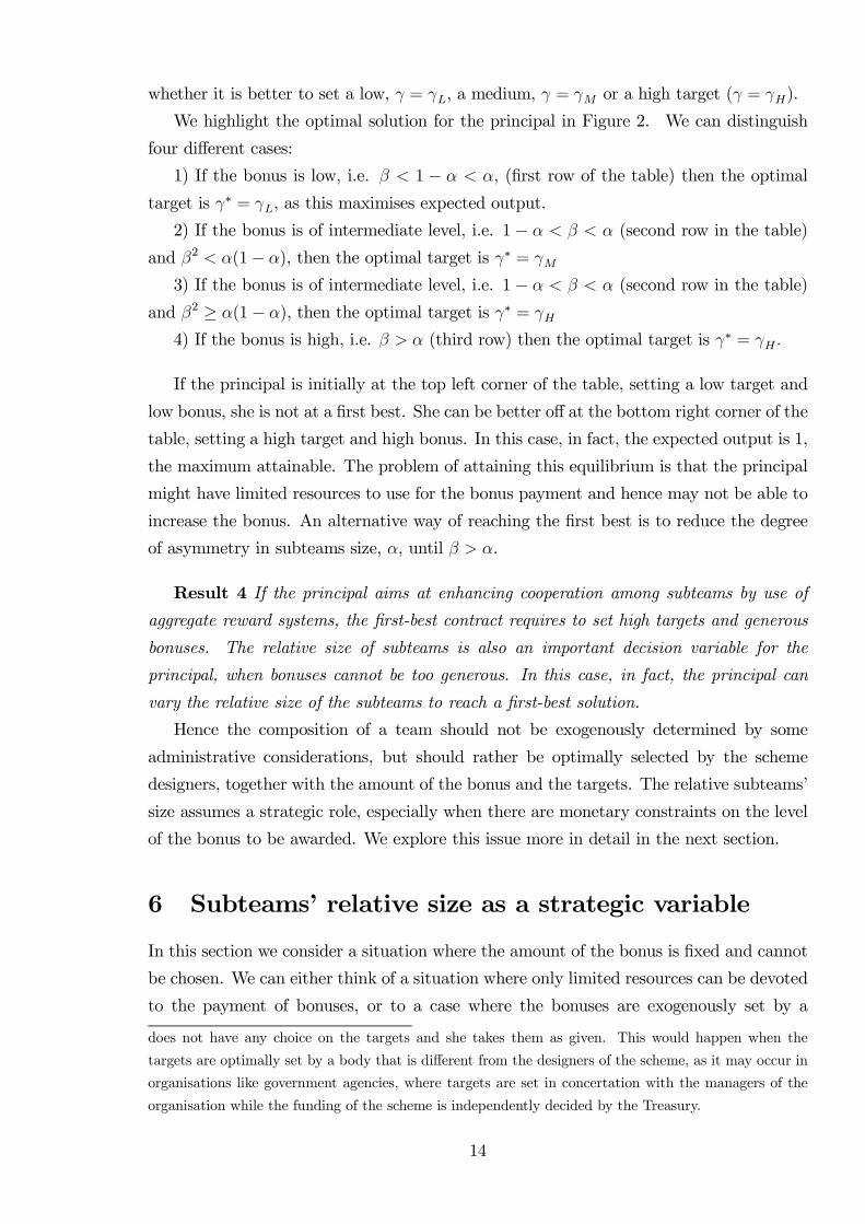
In Figure 3, we represent the four regions where the bonus can lie, as a function of α.

For each of these four regions we report the information on the value of optimal expected

output, the optimal target and the corresponding probability of reaching the target. This

latter depends on the value of the target and is calculated by substituting the optimal

effort choice of each subteam in equations (3)-(5).When β = β < 1

2, the first-best cannot

α

β

2

1

2

1

1

αβ −=1

)1(2 ααβ −=

αβ =

1

4

2

3

αβ −<1L

)1(2 ααβ −<

αβα <<− M1

αβα <<− M1

)1(2 ααβ −>

αβ >H

H

P

Q

=

=

=

*

*

*

1

1

γ

H

P

Q

=

=

−+=

*

*

* )1(

γ

α

β

αβ

MPQ === ***, , γ

α

ββ

L

P

Q

=

−−

−++−=

−−

−−+=

*

22

223

*

2

22

*

])1([

]33[

)1(

])1([

γ

βαα

ααβααβββ

βαα

βααββ

1α 2α

Figure 3: Optimal expected output, probability of success and target for each range of β

and different α.

be attained, as the bonus is too low and there is no margin to adjust the value of alpha

to get a first-best, i.e. such that β > α.

In this scenario, there are three possibilities:

1) If the bonus is low, i.e. β < 1 − α (this corresponds to region 1 in Figure 3), the

optimal target is low, γL, the effort choices of the two subteams are negatively related

and the expected output is:

Q∗ =β [α2 + (1− α)2 − β]

α (1− α)− β2

which is increasing in α.

9This is the case in the trial schemes we mentioned above, where the amount of the bonus was decided

by the Treasury for all three government agencies.

15

2) For (1− α) < β < α, and β2 < α(1−α) (this corresponds to region 2 in Figure 3),

the optimal target is medium, γM , the effort choice of the two subteams are independent

and the expected output is constant and equal to:

Q∗ = β

3) For (1 − α) ≤ β < α, and β2 > α(1 − α) (this corresponds to region 3 in Figure

3), the optimal target is high, γH , the two subteams cooperate in the effort choice and

expected output is decreasing in α.

Q∗ = β + (1− α)

If we compare these three levels of output, the highest is Q∗ = β+ (1−α) when β2 =

α(1−α). For β2 > α(1−α), Q∗starts decreasing if we increase alpha. For β2 < α(1−α),

Q∗is increasing in alpha.

In terms of Figure 3, if we fix a value of β = β < 1

2and start with two symmetric

subteams, α = 1

2, the expected output for the principal can be increased by increasing

alpha. In fact, up to α1 (region 1) expected output is an increasing function of alpha.

Between α1 ≤ α < α2, (region 2) the expected output is Q∗ = β and above α2 (region

3) it starts decreasing with alpha. The highest output is at α2,when β2 = α(1− α) and

Q∗ = β + (1− α).

Hence the best solution for the principal, faced with a limited budget for the bonus

at β < 1

2, is to set a high target and a sufficiently high degree of asymmetry in subteams’

size (such that β2 = α(1−α) ). A lower degree of asymmetry does not lead to subteams’

cooperation - as either i) the conditions (1 − α) < β < α and β2 < α(1 − α) hold and

subteam effort is independent, or ii) the condition β < 1− α holds and the effort choices

of the subteams are substitutes. A degree of asymmetry that is higher than β2 = α(1−α)

does involve cooperation across subteams, but provides a lower output to the principal.

Note that in the absence of a financial constraint on the level of the bonus, i.e. β ≥ 1

2,

a more symmetric size is preferable to the principal. In fact, if α = 1

2we can be sure to be

in region 4 of Figure 3, where a first-best can be reached. A higher degree of asymmetry

can instead lead to region 3, where expected output is lower.

In the schemes we mentioned in section 2, the relative size of the subteams was not

chosen by the scheme designers, but was exogenously taken as an organisational feature

of the public agency. The bonus was set by the HM Treasury. Although we can imagine

the scheme designers were involved in the decision about the level of the bonus, they

surely did not have complete control over its level. Hence it is possible that the incentive

schemes were not optimally set to induce greater cooperation across offices.

16

Testing the predictions of our theoretical model using the empirical evidence from

the schemes we mentioned above is not so straightforward. One very important issue of

those schemes, which is absent in our model, is the multitasking problem. The bonus

was awarded only if all or at least a set of the incentive targets were met, depending on

the organisation. In our model we abstract from multitasking issues in order to focus

on the role of subteams’ relative size on their effort choice. Nevertheless, we can look

at which were the teams among the incentivised ones who hit their incentive targets and

examine whether more/less symmetric teams were more likely to hit their targets. We can

also check how the degree of asymmetry in team size and the level of the target affected

subteams’ output. We do this in the next section.

7 Empirical evidence from Jobcentre Plus

Among the schemes introduced in the UK government agencies we mentioned above,

we select the Jobcentre Plus scheme, as this is the only scheme for which two different

incentive target levels were used. Jobcentre Plus is also the only public agency for which

we have office-level (sub-teams level) data.

Jobcentre Plus was launched in October 2001, amalgamating the functions of two agen-

cies: the Benefits Agency (BA), responsible for administering benefits to the unemployed,

lone parents and others, and the Employment Service (ES), responsible for job placement.

The method of delivering these services also began to change with the introduction in No-

vember 2001 of 56 new ’Pathfinder’ offices providing an integrated service, combining the

work of the original, separate, benefits offices and employment offices. This major reor-

ganisation meant redesigning districts, setting new performance targets and changing the

way of delivering business. The incentive scheme ran from April 2002 to April 2003, in 17

out of the 90 districts. These 17 districts (teams) were selected on the basis of containing

at least one Pathfinder office. The incentivised districts were grouped into two categories:

Band A districts, which contained up to 20% of Pathfinder offices over the total number

of offices, and Band B districts, with more than 21% of Pathfinder offices. Two different

target levels were applied to the two categories: for Band A districts the incentive target

consisted of 5% increase in the baseline output target (PSA target), whereas for Band

B districts it was a 7.5% increase. The incentive scheme included targets for five differ-

ent functions: job placements, customer service, employer service, other business delivery

functions, and reducing benefit calculation error and fraud. In this analysis we shall fo-

cus on the outcome job placements, as it is the only quantitative outcome measured at

office level. Job placements, job entries in Jobcentre Plus’ terminology, are measured as

weighted numbers of clients who are found work by the office. This measure is based on a

points system, which varies with the priority of the clients as imposed by the government

17

- for example, a jobless lone parent attracts 12 points, compared to 4 points for a short-

term unemployed claimant, and 1 point for an already-employed worker. Extra points

also accrue if the worker is not back on unemployment benefit within four weeks, and also

in certain priority areas. In the analysis below we shall consider job entry points as the

output of an office, as this is the measure used to assess performance for the incentive

scheme. Nine of the incentivised districts were Band A districts10 and the remaining eight

districts were Band B districts11. There were 962 offices producing job entries in total. Of

these, 740 were not incentivised and 222 were incentivised. Of the 222, 74 were in Band

B districts, whereas the remaining 148 were in Band A districts.

We first consider the incentivised teams and distinguish between those who hit their

targets for job entries and those who didn’t. We do this with a view to see whether the

level of the target and the office size dispersion had a clear role for the success of the

team. The questions we address are: 1) Are the successful teams composed by offices of

similar size? 2) Are the successful teams concentrated in the Band B districts (those who

were assigned a higher target)?.

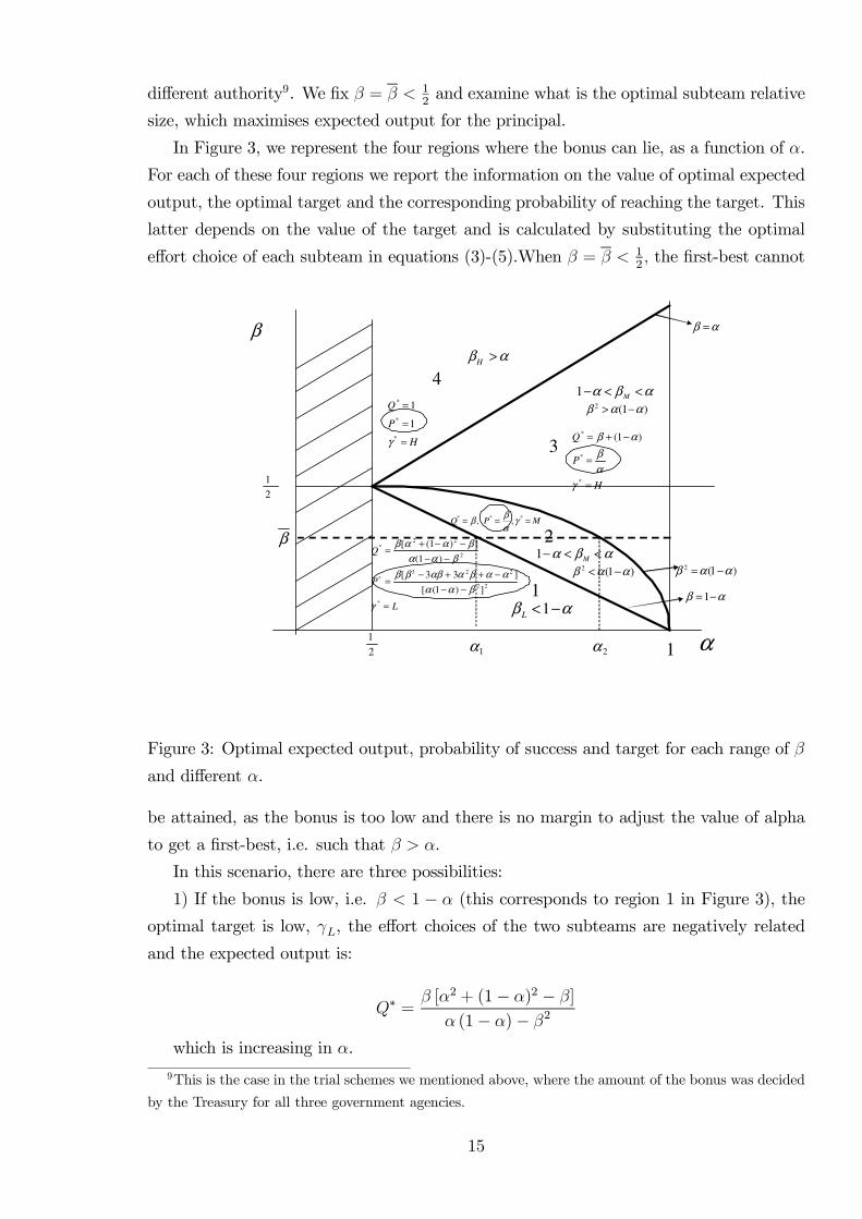
Unfortunately we only deal with a very small sample size, which is going to limit

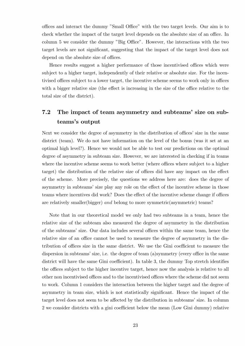
our analysis. In Table 1 we consider how the dispersion in office size varied across all

incentivised districts, distinguishing those districts who reached their targets with an

asterisk (and in bold red). We choose the Gini coefficient as a measure of dispersion

of office size in each district. On this purpose, for each district, we ranked offices from

small to large and calculated the cumulative percentage of staff in the offices and the

cumulative distribution of offices. An index equal to zero would mean perfect equality in

office size within the district, whereas an index equal to one would mean the total staff

is concentrated in one office. So we have one Gini coefficient for each district. The

Gini coefficient varies from 0.24 and 0.5712. If we divide the interval [0, 1] of the Gini

coefficient into quantiles, the incentivised teams who managed to reach the targets have

values concentrated in the second quantile, though the number of observations prevent

us from drawing any solid insights into how asymmetry in team size might have affected

the likelihood of hitting the targets. Three of the five successful districts (Bridgend,

Grampain and Wirral) were in Band B districts, whereas two (Manchester and Lothian)

were in Band A districts. Hence, also for the role of the target level on the team’s success,

we do not obtain a clear pattern.

As an alternative measure of office size asymmetry we considered a measure of dom-

10Band A districts were: Birmingham and Solihull, Derbyshire, Devon, Essex, Hampshire, London

Central South, Lothian and Borders, Manchester, Renfrews Inverclyde Argyll Bute.11Band B districts were: Bridgend, Calderdale, East Lacashire, Gateshead, Grampian, London North

West, Shropshire and Wirral.12The lowest value of the Gini coefficient in the non-incentivised teams is 0.16 and the highest is 0.62.

18

.57RENFREWS INVERCLYDE ARGYLL BUTE

.52DERBYSHIRE

.49LOTHIAN AND BORDERS

.48GATESHEAD AND SOUTH TYNESIDE

.47GRAMPIAN MORAY ORKNEY SHETLAND

.44ESSEX

.42SHROPSHIRE

.42CALDERDALE AND KIRKLEES

.41HAMPSHIRE

.40DEVON

.39WIRRAL

.37EAST LANCASHIRE

.36LONDON NORTH WEST

.34BRIDGEND AND RHONDDA CYNON TAF

.29BIRMINGHAM AND SOLIHULL

.26MANCHESTER

.24LONDON CENTRAL SOUTH

GiniDistrict

Figure 4: Table 1: The Gini coefficient in the incentivised districts at Jobcentre Plus

inance. For each district, we ranked each office within the district by their size. The n

largest offices per district were selected; where n = 25% of total offices (so in a district

with 4 offices, the largest 1 is selected). The sum of staff in the n offices was taken as

a percentage of total staff in the district, obtaining in this way a measure of dominance

which goes from 0 to 1. However, also in this case, we were not able to draw any clear

conclusion on the role of team asymmetry on the likelihood of hitting the targets. The

incentivised teams who hit the targets do not have a specific degree of dominance that

distinguishes them from those who did not hit the targets. One possibility is that the

sample size undermines our analysis. In what follows, we consider the office output as a

proxy for the effort choice of each sub-team, in order to check how the target level and

the team asymmetry affects the office response to the incentive scheme.

7.1 Impact of different target levels on the subteams’ outcome

In this section we consider the impact of the target level on the office’s output. Given that

we are going to estimate the impact of the incentive scheme on output it is important to

clarify how offices were selected to the treatment and how we intend to identify this effect.

As already mentioned, the 17 incentivised districts were selected into treatment on the

basis of containing at least one Pathfinder office. The choice of which office was to become

a Pathfinder office was based on the rationale that the locations of the Pathfinder offices

were to be spread across all 11 Jobcentre Plus regions. The specific sites in each region

were chosen by Field Directors and their District Managers on the grounds that their

19

management would be able to cope well with the demands of the new structure. Also,

the selected offices were to reflect a ”cross-section of different communities and customer

bases, i.e. from large inner-city offices to those in smaller towns, suburbs and rural

areas.”13 This suggests that the treatment assignment is stratified random: it is indeed

correlated to outcomes for Pathfinder offices, given the choice made on their location.

However, it is likely that assignment is random for all the other offices as these are in

the pilot incentive scheme because they are in the same district as the Pathfinder offices,

hence on grounds entirely unrelated to their own performance and characteristics14. One

could argue against this argument with the view that some of the districts might have

been more prepared than others for the structural change, thanks to a good district

manager or to the presence of good offices overall, and hence might have been chosen

on those grounds. According to this view, all offices within a Pathfinder district would

systematically perform better than others even without the incentive scheme. However,

the fact that the selected Pathfinder offices had to reflect a cross-section of different

communities and customer bases limits these arguments, as the emphasis was more on

the customers of the organisation rather than the quality of the office. Also, the fact that

offices tend to be self-contained and there are few operational links between offices in a

district rules out any kind of spillover-effects of good performing offices on the rest of the

district. Obviously, it would be ideal to test any systematic difference in the quality of

offices across districts before the introduction of the incentive scheme, but we cannot do it

in the absence of past data on performance, as the districts were redesigned shorty before

the introduction of the scheme. Therefore, in what follows we assume random assignment

to treatment for offices other than Pathfinder offices and we include in our analysis all

offices except for Pathfinder offices.

We consider the (log) job entry points as the output of an office. We run OLS re-

gressions using monthly data at office level. In order to isolate the effect of the incentive

scheme, we control for office characteristics that may affect output but are not due to

the incentive scheme. In particular, we control for the type and size of office, the quality

of staff and the labour market conditions. For the type of office, we distinguish between

Headquarter (HQ) offices and other offices, in that Headquarter offices had central ad-

ministrative functions and hence were a bit different than other offices. We also control

for any organisational change during the period of observation: the dummy jcp status is

to pick up the fact that during the observation period offices may have become Jobcen-

tre Plus offices (with the same organisational structure of the Pathfinder offices). As a

13Private communication.14We were informed that there are few operational links between offices in a district. In particualr, the

work of non-Pathfinder offices is largely unaffected by the presence of Pathfinder offices in the districts,

and different offices are largely self-contained.

20

measure of the quality of staff, we consider the private-public wage gap in the local area

- a high wage gap implying a lower quality workers in the public sector. The state of

demand in the labour market is measured as the ratio of the inflow of vacancies relative

to job seekers15. Questions we want to address are: once we control for any observable

influences on office performance, can we detect a different impact of the scheme on office

performance depending on the level of the target? Is the impact of the target level affected

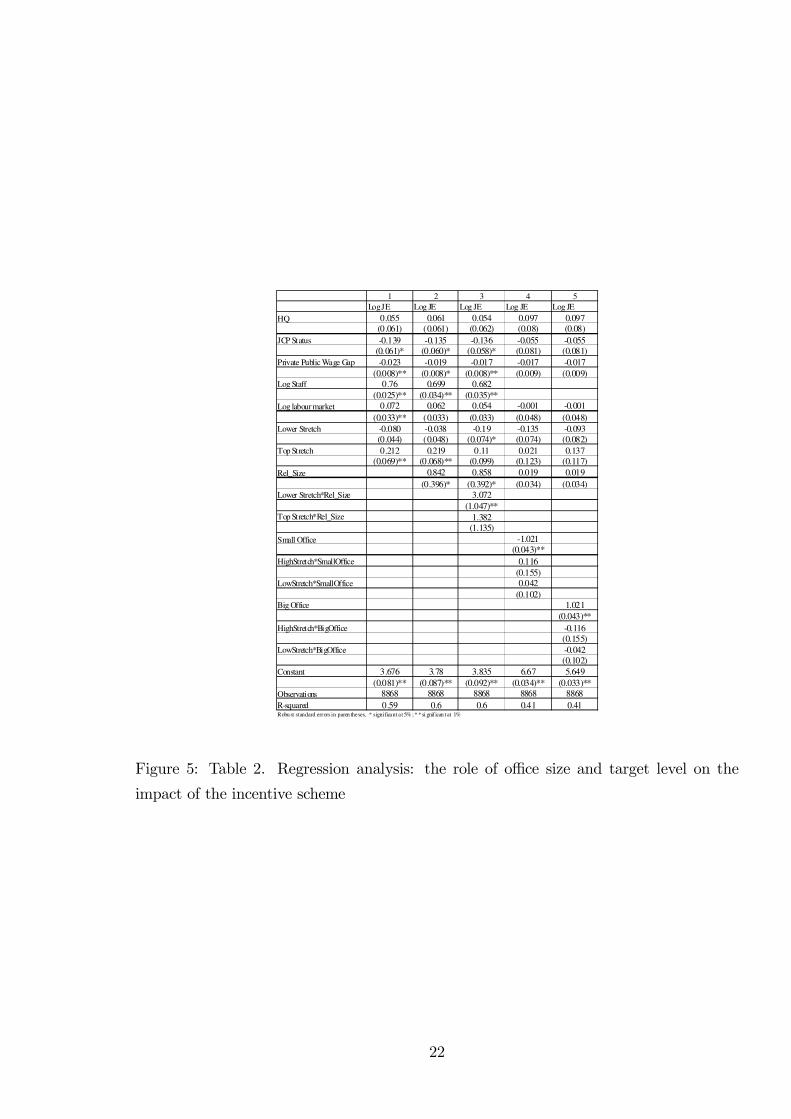
by the absolute and relative office size? Table 2 presents our results16.

Column 1 in Table 2 considers the impact of the target level on the output measure.

The dummy Lower stretch identifies the incentivised offices which were subject to the

lower target (5% stretch on annual performance as defined by the PSA target), whereas

the dummy Top stretch identifies the incentivised offices which were subject to the higher

target (7.5% stretch). Hence the analysis is relative to non-incentivised offices. Results

suggest a significative difference of the impact of the two target levels on offices’ perfor-

mance. A low target does not seem to have a statistically significant impact on output,

whereas the higher target positively affects output. In columns 2 and 3 we consider the

office relative size, defined as the ratio of staff in the office over the total staff in the

district where the office is located. Results on the interactions between the office relative

size and the target level in column 3 suggest that the impact of the higher target is not

affected by the relative size, whereas offices subject to the lower stretch tend to do better

if their relative size is bigger. This could confirm the theoretical prediction of Result 1,

according to which, when the target level is low, greater effort by one office induces lower

effort by the other office and it is possible that a smaller office contributes less than a big-

ger office, given that the expected return to effort is smaller, i.e. the impact of a marginal

increase in effort on the probability of reaching the target is less than for a bigger office.

In columns 4 and 5 we consider the absolute size and distinguish between big and small

offices, a big offices being an office with a bigger size than the average size (calculated

across all offices in all districts). In column 4 we consider small offices relative to big

15Our variable is derived from the Labour Force Survey Small Areas dataset. We constructed the

wage gap between the private sector and the public sector for each local authority looking at the relative

hourly wage of full-time workers. This was matched to the office postcode. Using the postcode (zip

code) for each JP office, we locate each office in a Travel To Work Area (TTWA98). We then extract

claimant inflow and vacancy inflow data from NOMIS for each TTWA and for each month. Whilst the

matching function uses the unemployment and vacancy stocks, we cannot take these as exogenous as they

are influenced by the outflow rate, our dependent variable. So we use the inflow, both of unemployed

claimants and of vacancies, and take the latter divided by the former. Note that the state of the labour

market plays two roles - first it provides the ’raw material’ necessary for the office to produce job entries.

Second, it proxies labour market tightness and hence the ease or otherwise of placing claimants in jobs.16We also control for time trends and consider dummies for each of the nine months of the incentive

scheme. We omit the results for lack of space. These are available at request from the authors.

21

1 2 3 4 5

Log JE Log JE Log JE Log JE Log JE

HQ 0.055 0.061 0.054 0.097 0.097

(0.061) (0.061) (0.062) (0.08) (0.08)

JCP Status -0.139 -0.135 -0.136 -0.055 -0.055

(0.061)* (0.060)* (0.058)* (0.081) (0.081)

Private Public Wage Gap -0.023 -0.019 -0.017 -0.017 -0.017

(0.008)** (0.008)* (0.008)** (0.009) (0.009)Log Staff 0.76 0.699 0.682

(0.025)** (0.034)** (0.035)**

Log labour market 0.072 0.062 0.054 -0.001 -0.001

(0.033)** (0.033) (0.033) (0.048) (0.048)

Lower Stretch -0.080 -0.038 -0.19 -0.135 -0.093

(0.044) (0.048) (0.074)* (0.074) (0.082)

Top Stretch 0.212 0.219 0.11 0.021 0.137

(0.069)** (0.068)** (0.099) (0.123) (0.117)

Rel_Size 0.842 0.858 0.019 0.019

(0.396)* (0.392)* (0.034) (0.034)

Lower Stretch*Rel_Size 3.072

(1.047)**Top Stretch*Rel_Size 1.382

(1.135)

Small Office -1.021

(0.043)**

HighStretch*SmallOffice 0.116

(0.155)

LowStretch*SmallOffice 0.042

(0.102)Big Office 1.021

(0.043)**

HighStretch*BigOffice -0.116

(0.155)

LowStretch*BigOffice -0.042

(0.102)

Constant 3.676 3.78 3.835 6.67 5.649

(0.081)** (0.087)** (0.092)** (0.034)** (0.033)**

Observations 8868 8868 8868 8868 8868

R-squared 0.59 0.6 0.6 0.41 0.41Robust standard errors in paren theses, * significant at 5% ; * * si gnif ican t at 1%

Figure 5: Table 2. Regression analysis: the role of office size and target level on the

impact of the incentive scheme

22

offices and interact the dummy ”Small Office” with the two target levels. Our aim is to

check whether the impact of the target level depends on the absolute size of an office. In

column 5 we consider the dummy ”Big Office”. However, the interactions with the two

target levels are not significant, suggesting that the impact of the target level does not

depend on the absolute size of offices.

Hence results suggest a higher performance of those incentivised offices which were

subject to a higher target, independently of their relative or absolute size. For the incen-

tivised offices subject to a lower target, the incentive scheme seems to work only in offices

with a bigger relative size (the effect is increasing in the size of the office relative to the

total size of the district).

7.2 The impact of team asymmetry and subteams’ size on sub-

teams’s output

Next we consider the degree of asymmetry in the distribution of offices’ size in the same

district (team). We do not have information on the level of the bonus (was it set at an

optimal high level?). Hence we would not be able to test our predictions on the optimal

degree of asymmetry in subteam size. However, we are interested in checking if in teams

where the incentive scheme seems to work better (where offices where subject to a higher

target) the distribution of the relative size of offices did have any impact on the effect

of the scheme. More precisely, the questions we address here are: does the degree of

asymmetry in subteams’ size play any role on the effect of the incentive scheme in those

teams where incentives did work? Does the effect of the incentive scheme change if offices

are relatively smaller(bigger) and belong to more symmetric(asymmetric) teams?

Note that in our theoretical model we only had two subteams in a team, hence the

relative size of the subteam also measured the degree of asymmetry in the distribution

of the subteams’ size. Our data includes several offices within the same team, hence the

relative size of an office cannot be used to measure the degree of asymmetry in the dis-

tribution of offices size in the same district. We use the Gini coefficient to measure the

dispersion in subteams’ size, i.e. the degree of team (a)symmetry (every office in the same

district will have the same Gini coefficient). In table 3, the dummy Top stretch identifies

the offices subject to the higher incentive target, hence now the analysis is relative to all

other non incentivised offices and to the incentivised offices where the scheme did not seem

to work. Column 1 considers the interaction between the higher target and the degree of

asymmetry in team size, which is not statistically significant. Hence the impact of the

target level does not seem to be affected by the distribution in subteams’ size. In column

2 we consider districts with a gini coefficient below the mean (Low Gini dummy) relative

23

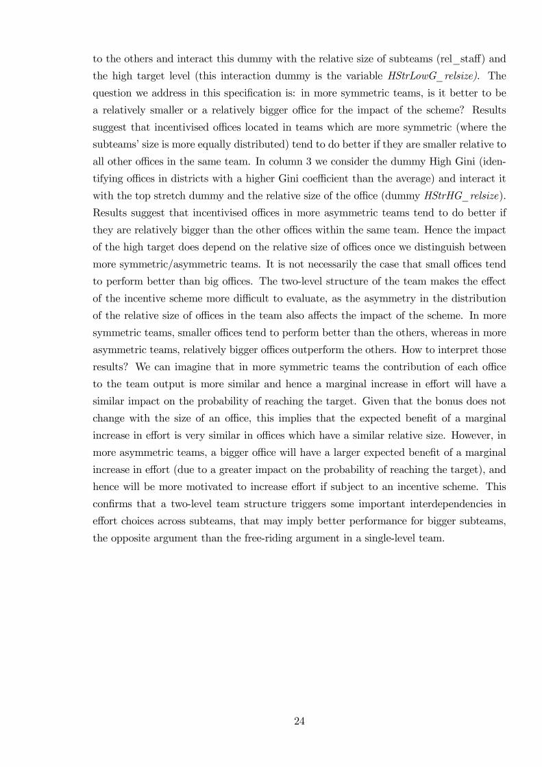
to the others and interact this dummy with the relative size of subteams (rel_staff) and

the high target level (this interaction dummy is the variable HStrLowG_relsize). The

question we address in this specification is: in more symmetric teams, is it better to be

a relatively smaller or a relatively bigger office for the impact of the scheme? Results

suggest that incentivised offices located in teams which are more symmetric (where the

subteams’ size is more equally distributed) tend to do better if they are smaller relative to

all other offices in the same team. In column 3 we consider the dummy High Gini (iden-

tifying offices in districts with a higher Gini coefficient than the average) and interact it

with the top stretch dummy and the relative size of the office (dummy HStrHG_relsize).

Results suggest that incentivised offices in more asymmetric teams tend to do better if

they are relatively bigger than the other offices within the same team. Hence the impact

of the high target does depend on the relative size of offices once we distinguish between

more symmetric/asymmetric teams. It is not necessarily the case that small offices tend

to perform better than big offices. The two-level structure of the team makes the effect

of the incentive scheme more difficult to evaluate, as the asymmetry in the distribution

of the relative size of offices in the team also affects the impact of the scheme. In more

symmetric teams, smaller offices tend to perform better than the others, whereas in more

asymmetric teams, relatively bigger offices outperform the others. How to interpret those

results? We can imagine that in more symmetric teams the contribution of each office

to the team output is more similar and hence a marginal increase in effort will have a

similar impact on the probability of reaching the target. Given that the bonus does not

change with the size of an office, this implies that the expected benefit of a marginal

increase in effort is very similar in offices which have a similar relative size. However, in

more asymmetric teams, a bigger office will have a larger expected benefit of a marginal

increase in effort (due to a greater impact on the probability of reaching the target), and

hence will be more motivated to increase effort if subject to an incentive scheme. This

confirms that a two-level team structure triggers some important interdependencies in

effort choices across subteams, that may imply better performance for bigger subteams,

the opposite argument than the free-riding argument in a single-level team.

24

1 2 3

Log JE Log JE Lo g JE

H Q 0.0 59 0.09 7 0.0 97

(0.0 61 ) ( 0.07 9) (0.0 79)

J C P Statu s -0 .19 2 0.11 7 0.1 17

(0 .0 55 )** ( 0.07 5) (0.0 75)

P rivate Pu blic W age G ap -0 .02 4 0.01 6 0.0 16

(0 .0 08 )** ( 0.00 9) (0.0 09)

L og Lab ou r M ar ket 0.07 -0 .1 04 - 0.10 4

(0. 0 33 )* (0.0 45) * (0 .0 45 )*

L og Staff 0.7 61

(0 .0 26 )**

T op Stretch 0.89 -0 .1 33 - 0.13 3

(0. 4 17 )* ( 0.12 4) (0.1 24)

g ini 0.0 26

(0.1 54 )

H igh S tretc h_ gin i -1 .60 4

(1.0 08 )

rel_ staff 5.46 8 6.23

(0. 57 3) ** (0 .4 12 )**

L owG in i 0.14 6

(0.0 73) *

h igh tg _rel size 4.59 2 0.77

(1. 23 9) ** (1.5 86)

L owG in i_ rels iz e 0.76 2

( 0.69 7)

H StrL owG _re lsize -3 .8 21

(1. 37 2) **

H igh Gin i - 0.14 6

(0 .0 73 )*

H igh Gin i_ relsize - 0.76 2

(0.6 97)

H StrH G _relsize 3.8 21

(1 .3 72 )**

C on stan t 3.6 55 5.41 2 5.5 59

(0 .1 11 )** (0. 06 1) ** (0 .0 46 )**

O bservatio ns 8 86 8 88 68 8 86 8

R -s qu ared 0.59 0 .4 0 . 4

Ro bust s tandard erro rs i n parent heses ; * s ign if icant at 5 %; * * si gni fi can t a t 1%

Table 3. Teams’ asymmetry, subteams size and the impact of the incenitve scheme.

8 Conclusion

We have considered the implications of setting incentive schemes for teams defined by

the reward system and based on administrative boundaries, comprising different units of

production (subteams). In a simple two-subteam model, we show that the way the scheme

is designed creates important interdependencies in the effort choice between subteams

and setting targets on aggregate output does not necessarily create cooperation among

sub-teams. In fact, we show that interdependencies in effort choice depend on the level

of the target: if the target is low enough (relative to the subteams’ output) so that it

can be reached by one of the two sub-teams, then the optimal choice of each sub-team

is negatively affected by the other sub-team’s effort and cooperation has to be induced

externally, for example by some form of monitoring. For a medium level of the target,

subteams’ efforts are independent and only when high targets are set, a greater effort

by one subteam induces greater effort by the other subteam. We derive the optimal

solution for the principal, which requires setting high targets and high bonuses. When

high bonuses can be awarded, then the degree of asymmetry in subteams’ size should

be minimum and should guarantee that the value of the bonus is higher than the value

25

of the output of the biggest sub-team. If the principal faces financial constraints and

cannot freely set the level of the bonus, then a first-best solution cannot be achieved. In

this case, the relative size of sub-teams becomes a crucial variable to deliver incentives.

The principal can adjust the relative size of subteams to increase expected output. The

second-best requires a critical value of the subteams’ relative size, which should not be

perfectly symmetric. Hence the way the team is designed (dispersion in sub-units size) is

very important for the final outcome of the scheme, above all when the principal cannot

freely set the level of the bonuses. This implies that teams should not be exogenous:

their composition (relative size of sub-units) should be optimally selected by the scheme

designers.

Using data for one of the incentive schemes implemented in a public organisation

in the UK, we consider the effects of two different target levels on subteams’ (offices’)

output. Results confirm the theoretical predictions that incentivised offices outperform

non-incentivised offices only in teams with a higher target level. We also find that in

districts with a lower (than average) degree of asymmetry in sub-teams size, the relative

size of offices negatively affects performance. Whereas in districts with a higher (than

average) degree of asymmetry, the scheme is more successful in relatively bigger offices.

This suggests that the impact of the scheme does indeed depend on the distribution of

offices’ size in the team and not only on their relative size. Moreover, bigger subteams

may outperform the others, suggesting that the argument in favour of a smaller size to

tackle free-riding issue does not necessarily apply in two-level teams and some conflicting

free-riding issues may be at work.

26

References

[1] S. Burgess, C. Propper, M. Ratto, E. Tominey, 2011.“Incentives in the Public Sector:

Evidence from a government Agency” , ), CMPO Working Paper 11/265.

[2] S. Burgess, C. Propper, M. Ratto, E. Tominey ”Evaluation of the Intro-

duction of the Makinson Incentive Scheme in Child Support Agency”, 2005

http://www.bristol.ac.uk/cmpo/events/2005/markinson/childsupport.pdf

[3] S. Burgess, C. Propper, M. Ratto, Stephanie von Hinke Kessler Scholder, E. Tominey,

2010 ”Smarter task assignment or greater effort: what makes a difference in team

performance?”, Economic Journal, Vol. 120 (547), 968-989.

[4] Che Yeon-Koo and Yoo Seung-Weon , 2001”Optimal Incentives for Teams”, American

Economic Review, Vol. 91 (3), 525-541.

[5] W. Encinosa III, M. Gaynor, J. Rebitzer, 2007 “The sociology of groups and the

economics of incentives: Theory and evidence on compensation systems”, Journal of

Economic Behavior & Organization, Vol. 62(2), 187-214.

[6] P. Francois, 2000 “’Public service motivation’ as an argument for government provi-

sion”, Journal of Public Economics 78, 275-299.

[7] B. Holmström, 1982. “Moral hazard in teams”, Bell Journal of Economics, 13, 324-

340.

[8] H. Itoh, 1991. “Incentives to help in multi-agent situations”, Econometrica, 59, (3),

611-636.

[9] E. Kandel- E. Lazear, 1992 “Peer Pressure and Partnerships”, Journal of Political

Economy, 100 (4), 801-817.

[10] J. Makinson “Incentives for change. Rewarding performance in national government

networks”, Public Service Productivity Panel, 2000.

[11] OECD ”Trends in Human Resources Management Policies in OECD Member coun-

tries: An Analysis of the Results of the OECD Survey on Strategic Human Resources

Management”, 2004a, (GOV/PGC/HRM(2004)2).

[12] OECD ”Performance Related Policies for Government Employees: Main Trends in

OECD Member Countries”, 2004b, (GOV/PGC/HRM(2004)1).

27