Teaching radioactive decay & radiometric dating: an analog activity based on fluid dynamics Lily L. Claiborne Calvin F. Miller Department of Earth & Environmental Sciences, Vanderbilt University Abstract We present a new laboratory activity for teaching radioactive decay using

hydrodynamic processes as an analog and an evaluation of its efficacy in the classroom.

A fluid flowing from an upper beaker into a lower beaker (shampoo in this case)

behaves mathematically identically to radioactive decay, mimicking the exponential

decay process, dependent on the amount of fluid in the upper beaker (representing the

amount of parent isotopes) and the size of the hole in the beaker (representing the decay

constant). Students measure the fluid depth with time for several “runs” with varied

conditions, then graph their results, create decay equations, manipulate these equations

and use them to “date” another experiment. They then apply their new understanding

to make predictions regarding complications involved in the decay process and its use

in dating (such as daughter loss). Student quiz performance improved from before to

after the activity, indicating improved student learning. Student comments and

questions indicated deep understanding and a new curiosity about the process and its

application.

Introduction

Understanding the process of radioactive decay and its use in radiometric dating

is necessary to understanding basic foundations of modern science and is essential

knowledge for educated citizenry concerned about current controversies over

evolution, the age of the earth, and the use of radioactive decay as an energy source. It

is, therefore, an important concept for students in secondary through graduate level

science courses to fully internalize. However, due to its very small scale, mathematical

treatment, and general unfamiliarity, the topic is fundamentally difficult for students to

grasp (Prather, 2005). Commonly, lectures accompanied by demonstrations are

employed to teach this topic, using games with dice, cards or poker chips (McGeachy,

1988; Kowalski, 1981; Clinikier, 1980), computer simulations (Jesse, 2003), electrical

circuitry (Wunderlich & Peastrel, 1978; Evans, 1974), or melting ice (Wise, 1990) to

mimic the process of decay and explain the concept of half-life. While these

demonstrations may illustrate the randomness and/or exponential nature of decay,

demonstrations, by their very nature, challenge student engagement. .

We present here a newly developed hands-on laboratory activity for teaching

radioactive decay and radiometric dating, and an evaluation of the activity’s

effectiveness. In this lesson, hydrodynamic principles and processes serve as an analog

for radioactive decay processes. Using analogies in teaching, such as the one employed

here, has been shown to be a highly effective teaching strategy (Duit, 1991). The use of

analogy makes this lesson particularly effective at instilling an intuitive understanding

of this complex, unfamiliar process and its uses by guiding students as they relate

radioactive decay to more familiar, intuitive and approachable processes of fluid flow.

The fundamentals that are learned can be adapted to appropriately address any level

classroom, from elementary through graduate courses. We have found it effective at all

levels of university education. In the analogy employed herein, students observe the

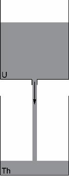
drainage of fluid from a container with a hole in its base into another container (Figure

1), and they recognize that this process can be described qualitatively and quantitatively

in exactly the same way as decay of radioactive parent isotopes and resulting

production of daughter isotopes. This allows students to observe, record, and

manipulate the process in a way impossible with real radioactive materials. They can

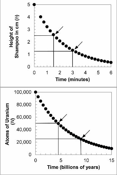
see the exponential decrease of flow from the upper beaker to lower with time (Figure

2a), and so clearly envision the exponential decay of radioactive isotopes and the

meaning of “half-lives” (Figure 2b). Students closely observe, measure, graph, and

think about the behavior of the fluid flow and then define the factors that control the

process, extract and manipulate the controlling equations, and make predictions

regarding changes to the initial conditions. They are then asked to transfer this

conceptual understanding to the process of radioactive decay. This connection to

familiar concepts and the ability to measure and manipulate the process promotes a

deep understanding of the decay process and its use in geochronology.

Theoretical Framework

Teaching with analogs

New ideas are best constructed by building on previously acquired knowledge

or by relating the unfamiliar to the familiar (Duit, 1991; Sibley, 2009). This makes

analogies particularly useful in teaching, as we use a concrete or familiar “source”

concept to essentially serve as a picture or metaphor that explains an abstract or

(b)

unfamiliar “target” concept (Dupin & Joshua, 1989; Duit, 1991). This is particularly

useful for geosciences, where many key concepts and processes are not visible or

apparent on the Earth’s surface or on human timescales (Jee et al., 2010). Along with

internalizing the target concept, as science students develop analogical reasoning skills,

they are mimicking the reasoning skills used by scientists to create and use models for

scientific phenomena (Sibley, 2009). These skills are essential for scientific literacy, and

lack of this understanding has been cited as one reason many students struggle with

science in general (White and Frederiksen, 1998).

While the use of analogies and analogical models (Jee et al., 2010) in teaching has

been shown to enhance student conceptual understanding and build essential scientific

reasoning skills, some inherent pitfalls must be avoided in order for the exercise to be

effective (Harrison & Treagust, 1993). The source concept or analog must be familiar to

the student, corresponding attributes between the source concept and target concept

must be explored, unshared attributes between the source concept and target concept

must be explicitly discussed, and the instructor must ensure that the students see the

source concept in the intended manner (Thagard, 1992; Duit, 1991; Orgill & Bodner,

2006).

In order to prevent these sorts of problems from rendering analogical lessons

ineffective, several researchers have developed explicit guidelines for teaching with

analogies. We have based our lesson on two of these sets of guidelines that we believe

best fit classroom practices and the practicalities of the analog activity we had in mind.

Dupin and Joshua (1989) describe guidelines for a “modeling analogy” which we

believe applies to our analog well, as it uses a hands-on physical model to relay the

source concept (see also Jee et al., 2010). The modeling analogy should have the

following five characteristics (Dupin & Joshua, 1989):

1. It serves as a picture or metaphor to put a new concept in concrete form. 2. It must have a “descriptive function” which helps students to understand the

target concept and to recognize that the explanation is plausible. 3. It must be less complex than the target concept. 4. It does not have to constitute a real situation. It can be idealized to encourage

thorough experiments so that students think deeply about the target concept. 5. The analogical system must have great structural similarity to the target concept,

such that it is adaptable to different teaching situations and depths of understanding.

Glynn (1991) proposed the following Teaching With Analogy (TWA) model that has

proven highly effective (Harrison and Treagust, 1993; see similar instructional supports

described in Jee et al., 2010), and on which we based the framework of our lesson:

1. Introduce target concept to be learned 2. Cue the students’ memory of the analogous situation 3. Identify the relevant features of the analog 4. Map the similarities between the analog and the target concepts 5. Identify the comparisons for which the analogy breaks down 6. Draw conclusions about the target concepts

Fundamentals: Radioactive Decay

Radioactive decay occurs when an unstable isotope, known as the ‘parent’ isotope,

emits radiation through loss of an ionizing particle from its nucleus. This transforms

the isotope into a new, ‘daughter’ isotope, often a different element. For example,

nuclei of 238U are unstable and by emitting alpha particles decay into 234Th (Faure and

Mensing, 2005). While the timing of the loss of a particle from an individual unstable

nucleus is random, over long periods of time and with large numbers of nuclei, the rate

of decay is measurable and constant. The decay process can be represented

mathematically by the following equation

where N is the amount of parent isotope, t represents time, is the decay constant for

the given isotopic system. Note that the decay rate of parent to daughter is constant for

each isotopic system, and is essentially a proportion per unit time. For example, the

rate of decay (decay constant) of 238U is 1.55x10-10/year (Faure and Mensing, 2005). This

is an exponential relationship, as shown by Figure 2b and the solution to the above

equation:

,

where N0 is the initial amount of parent. Because of the timescales involved and this

exponential nature of the process, it is useful to consider decay rates in terms of half-

life, or the amount of time it takes for half of the parent material to decay (Figure 2b).

For example, the half-life of 238U is 4.468 billion years (Faure and Mensing, 2005).

In radiometric dating, we measure the amount of parent and daughter isotope in

a material and, since the decay rates of radioactive isotopes are known, we can use the

above equation to calculate the time that has passed since the product of decay

(daughter) began to accumulate. The incorporation of non-radioactively produced

‘daughter’ isotopes at the formation of the material can occur in natural systems and

necessitates careful corrections to obtain accurate results. The loss of daughter isotopes

at some time after the formation of the material can also occur, for example, if the

material is heated sufficiently, and can be used to determine dates of thermal events

that cause the loss.

Fundamentals: A Hydrodynamic Analog for Radioactive Decay

The experiment carried out in this lesson allows students to explore a simple,

intuitive hydrodynamic principle in order to develop a qualitative and quantitative

understanding of radioactive decay. The experimental analog consists of one beaker

with a small hole in the base suspended above another beaker (Figure 1). Fluid flow

from the upper beaker to the lower beaker is controlled by the size of the hole and the

hydrostatic pressure being exerted by the column of fluid above. Rate of flow, and thus

change in height of fluid in the upper beaker with time, is directly proportional to both

the height of fluid in the beaker at any given time and the area of the hole in the bottom

of the beaker. This can be stated as:

where h is the height of fluid in the upper beaker, t is time, α is a flow coefficient that

includes the density and viscosity of the fluid, the acceleration due to gravity, the cross

sectional area of the beaker, and the area of the hole. The value is negative because the

height of fluid in the upper beaker is decreasing.

Radioactive decay is analogous to the flow of fluid out of the beaker, because the

rate of loss of parent isotope is directly proportional to the amount of parent present

(the height of fluid) and the decay constant (the flow coefficient α). The equation for

radioactive decay is therefore mathematically identical to the equation for fluid flow

shown above:

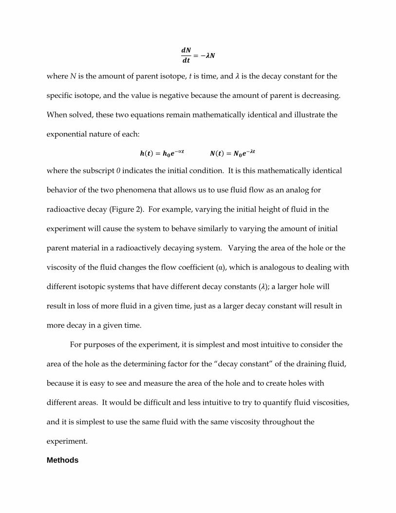
where N is the amount of parent isotope, t is time, and is the decay constant for the

specific isotope, and the value is negative because the amount of parent is decreasing.

When solved, these two equations remain mathematically identical and illustrate the

exponential nature of each:

where the subscript 0 indicates the initial condition. It is this mathematically identical

behavior of the two phenomena that allows us to use fluid flow as an analog for

radioactive decay (Figure 2). For example, varying the initial height of fluid in the

experiment will cause the system to behave similarly to varying the amount of initial

parent material in a radioactively decaying system. Varying the area of the hole or the

viscosity of the fluid changes the flow coefficient (α), which is analogous to dealing with

different isotopic systems that have different decay constants ( ); a larger hole will

result in loss of more fluid in a given time, just as a larger decay constant will result in

more decay in a given time.

For purposes of the experiment, it is simplest and most intuitive to consider the

area of the hole as the determining factor for the “decay constant” of the draining fluid,

because it is easy to see and measure the area of the hole and to create holes with

different areas. It would be difficult and less intuitive to try to quantify fluid viscosities,

and it is simplest to use the same fluid with the same viscosity throughout the

experiment.

Methods

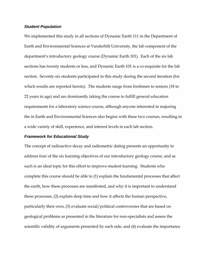
Student Population

We implemented this study in all sections of Dynamic Earth 111 in the Department of

Earth and Environmental Sciences at Vanderbilt University, the lab component of the

department’s introductory geology course (Dynamic Earth 101). Each of the six lab

sections has twenty students or less, and Dynamic Earth 101 is a co-requisite for the lab

section. Seventy-six students participated in this study during the second iteration (for

which results are reported herein). The students range from freshmen to seniors (18 to

22 years in age) and are dominantly taking the course to fulfill general education

requirements for a laboratory science course, although anyone interested in majoring

the in Earth and Environmental Sciences also begins with these two courses, resulting in

a wide variety of skill, experience, and interest levels in each lab section.

Framework for Educational Study

The concept of radioactive decay and radiometric dating presents an opportunity to

address four of the six learning objectives of our introductory geology course, and as

such is an ideal topic for this effort to improve student learning. Students who

complete this course should be able to (1) explain the fundamental processes that affect

the earth, how these processes are manifested, and why it is important to understand

these processes, (2) explain deep time and how it affects the human perspective,

particularly their own, (3) evaluate social/political controversies that are based on

geological problems as presented in the literature for non-specialists and assess the

scientific validity of arguments presented by each side, and (4) evaluate the importance

of scientific uncertainty in understanding the earth’s processes and what this means for

the future.

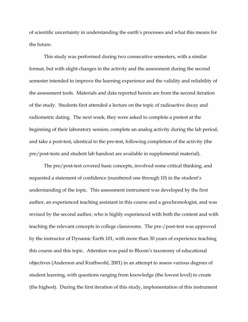
This study was performed during two consecutive semesters, with a similar

format, but with slight changes in the activity and the assessment during the second

semester intended to improve the learning experience and the validity and reliability of

the assessment tools. Materials and data reported herein are from the second iteration

of the study. Students first attended a lecture on the topic of radioactive decay and

radiometric dating. The next week, they were asked to complete a pretest at the

beginning of their laboratory session, complete an analog activity during the lab period,

and take a post-test, identical to the pre-test, following completion of the activity (the

pre/post-tests and student lab handout are available in supplemental material).

The pre/post-test covered basic concepts, involved some critical thinking, and

requested a statement of confidence (numbered one through 10) in the student’s

understanding of the topic. This assessment instrument was developed by the first

author, an experienced teaching assistant in this course and a geochronologist, and was

revised by the second author, who is highly experienced with both the content and with

teaching the relevant concepts in college classrooms. The pre-/post-test was approved

by the instructor of Dynamic Earth 101, with more than 30 years of experience teaching

this course and this topic. Attention was paid to Bloom’s taxonomy of educational

objectives (Anderson and Krathwohl, 2001) in an attempt to assess various degrees of

student learning, with questions ranging from knowledge (the lowest level) to create

(the highest). During the first iteration of this study, implementation of this instrument

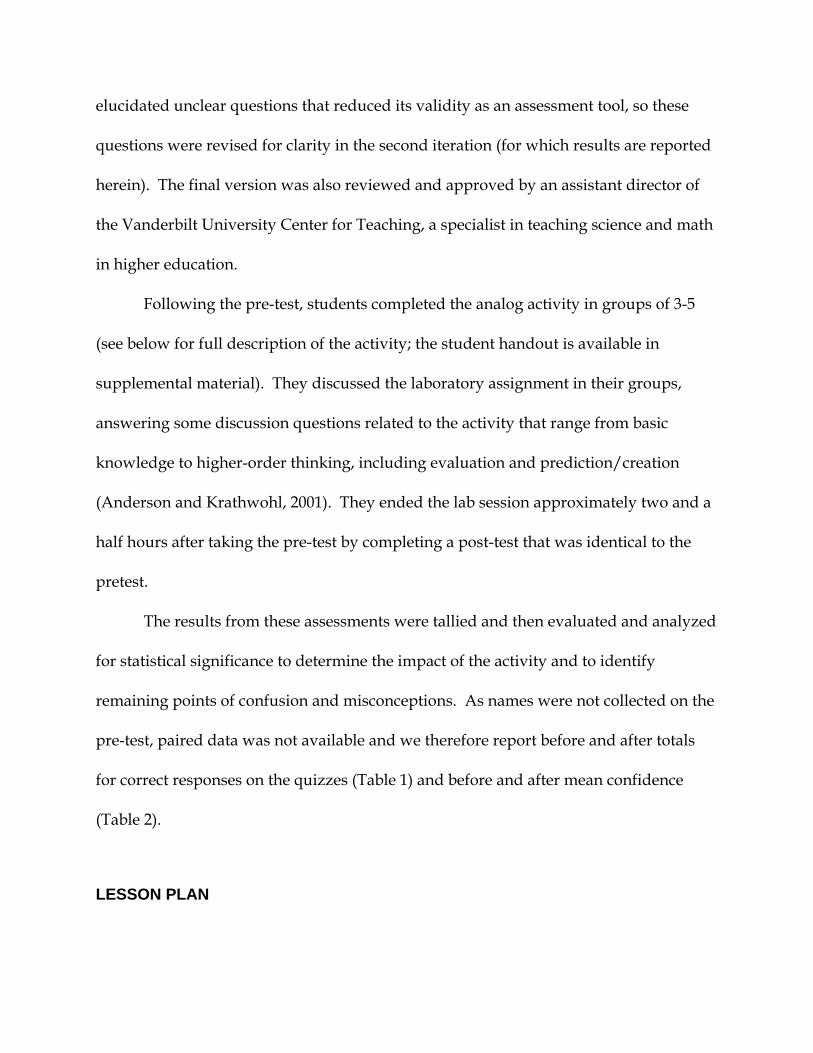
elucidated unclear questions that reduced its validity as an assessment tool, so these

questions were revised for clarity in the second iteration (for which results are reported

herein). The final version was also reviewed and approved by an assistant director of

the Vanderbilt University Center for Teaching, a specialist in teaching science and math

in higher education.

Following the pre-test, students completed the analog activity in groups of 3-5

(see below for full description of the activity; the student handout is available in

supplemental material). They discussed the laboratory assignment in their groups,

answering some discussion questions related to the activity that range from basic

knowledge to higher-order thinking, including evaluation and prediction/creation

(Anderson and Krathwohl, 2001). They ended the lab session approximately two and a

half hours after taking the pre-test by completing a post-test that was identical to the

pretest.

The results from these assessments were tallied and then evaluated and analyzed

for statistical significance to determine the impact of the activity and to identify

remaining points of confusion and misconceptions. As names were not collected on the

pre-test, paired data was not available and we therefore report before and after totals

for correct responses on the quizzes (Table 1) and before and after mean confidence

(Table 2).

LESSON PLAN

The student handout with instructions, material lists, and follow up questions is available in the

supplemental material.

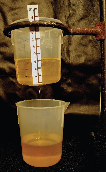
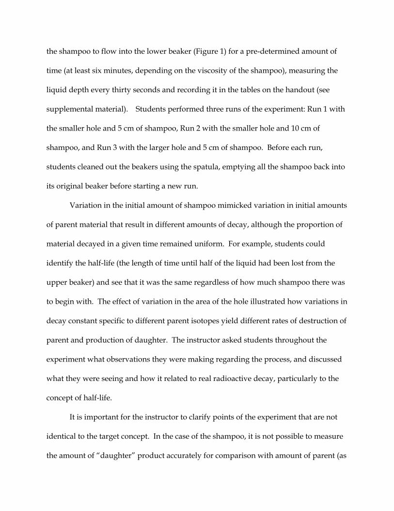
The analog activity employed 4 beakers of the same size (we used 250mL), two of

which had a hole in the base and vertical depth scales on the side (centimeters; Figure

1b). We used plastic beakers and a drill to form the holes; the exact size of the holes

does not matter as long as one is larger than the other (approximately double in size

worked well for us). Each group also used a beaker stand, modeling clay formed into a

stopper for the holes, baby shampoo (fill one beaker), a stopwatch, a spatula and access

to Microsoft Excel. We chose shampoo as our fluid for ease in cleanup. For the sizes of

holes that we used, we found that the discharge rate using baby shampoo (a function of

its viscosity) was particularly appropriate, resulting in changes in depth that were

readily measurable during the time available for the lab activity.

The supplemental material for the student handout has instructions for

completing the following activities and for follow-up questions to guide synthesis of the

ideas. The activity takes approximately ninety minutes.

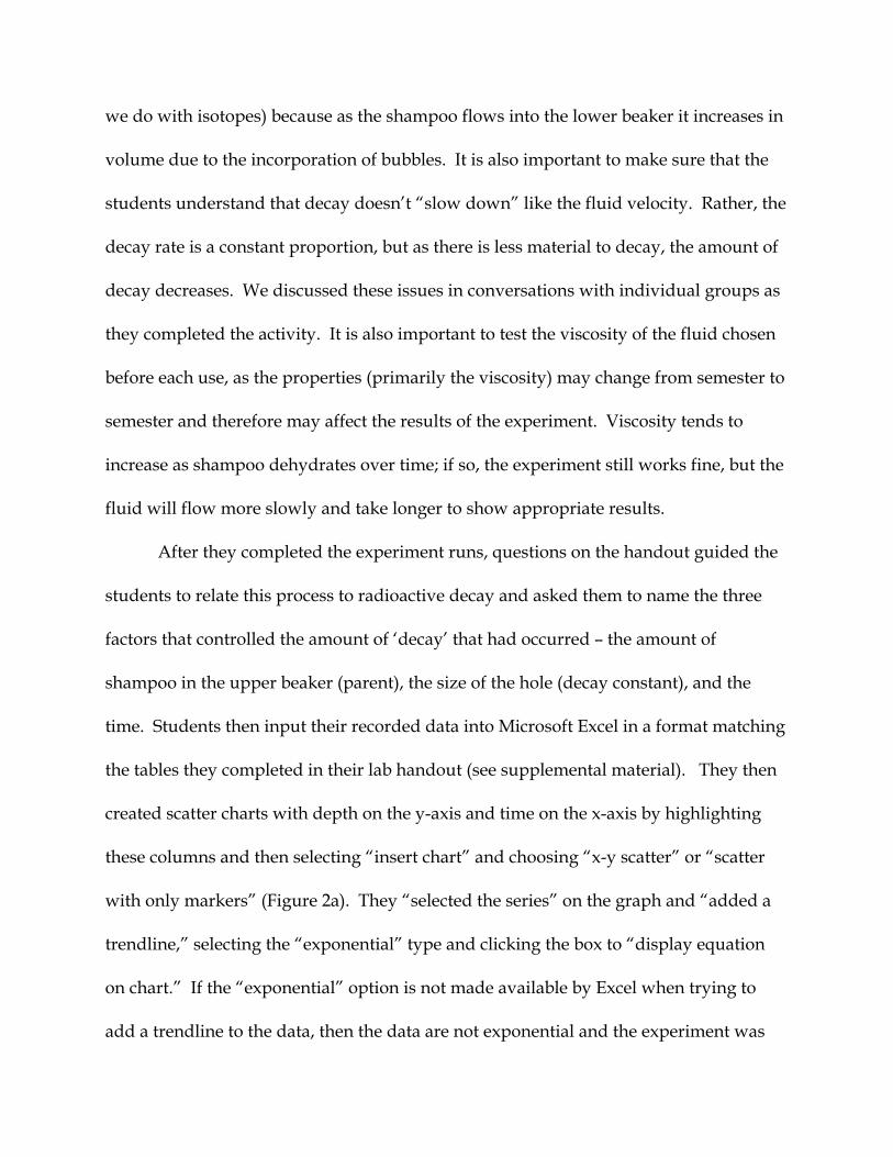
Students positioned the beaker with the smaller hole above a beaker with a solid

base using the beaker stand (Figure 1). Students plugged the hole with clay and poured

a pre-determined amount (depth in cm) of shampoo into the upper beaker. For their

first run, this was 5 cm. They were told that for the experiment, the shampoo in the

upper beaker represents the parent isotope, and the flow through the hole represents

the decay of the parent to produce the daughter isotope (shampoo in the lower beaker).

When they were ready to begin the experiment, they unplugged the hole and allowed

the shampoo to flow into the lower beaker (Figure 1) for a pre-determined amount of

time (at least six minutes, depending on the viscosity of the shampoo), measuring the

liquid depth every thirty seconds and recording it in the tables on the handout (see

supplemental material). Students performed three runs of the experiment: Run 1 with

the smaller hole and 5 cm of shampoo, Run 2 with the smaller hole and 10 cm of

shampoo, and Run 3 with the larger hole and 5 cm of shampoo. Before each run,

students cleaned out the beakers using the spatula, emptying all the shampoo back into

its original beaker before starting a new run.

Variation in the initial amount of shampoo mimicked variation in initial amounts

of parent material that result in different amounts of decay, although the proportion of

material decayed in a given time remained uniform. For example, students could

identify the half-life (the length of time until half of the liquid had been lost from the

upper beaker) and see that it was the same regardless of how much shampoo there was

to begin with. The effect of variation in the area of the hole illustrated how variations in

decay constant specific to different parent isotopes yield different rates of destruction of

parent and production of daughter. The instructor asked students throughout the

experiment what observations they were making regarding the process, and discussed

what they were seeing and how it related to real radioactive decay, particularly to the

concept of half-life.

It is important for the instructor to clarify points of the experiment that are not

identical to the target concept. In the case of the shampoo, it is not possible to measure

the amount of “daughter” product accurately for comparison with amount of parent (as

we do with isotopes) because as the shampoo flows into the lower beaker it increases in

volume due to the incorporation of bubbles. It is also important to make sure that the

students understand that decay doesn’t “slow down” like the fluid velocity. Rather, the

decay rate is a constant proportion, but as there is less material to decay, the amount of

decay decreases. We discussed these issues in conversations with individual groups as

they completed the activity. It is also important to test the viscosity of the fluid chosen

before each use, as the properties (primarily the viscosity) may change from semester to

semester and therefore may affect the results of the experiment. Viscosity tends to

increase as shampoo dehydrates over time; if so, the experiment still works fine, but the

fluid will flow more slowly and take longer to show appropriate results.

After they completed the experiment runs, questions on the handout guided the

students to relate this process to radioactive decay and asked them to name the three

factors that controlled the amount of ‘decay’ that had occurred – the amount of

shampoo in the upper beaker (parent), the size of the hole (decay constant), and the

time. Students then input their recorded data into Microsoft Excel in a format matching

the tables they completed in their lab handout (see supplemental material). They then

created scatter charts with depth on the y-axis and time on the x-axis by highlighting

these columns and then selecting “insert chart” and choosing “x-y scatter” or “scatter

with only markers” (Figure 2a). They “selected the series” on the graph and “added a

trendline,” selecting the “exponential” type and clicking the box to “display equation

on chart.” If the “exponential” option is not made available by Excel when trying to

add a trendline to the data, then the data are not exponential and the experiment was

not successful. This only occurred in cases where students somehow disturbed the

experiment in mid-run (spilling, for example) and then continued collecting data. This

was repeated for each run, resulting in three graphs and three equations.

The students then dissected these equations, answering questions on the

handout that require them to define what each number represented (see supplemental

material), and concluding that the numbers in the equation that described their data

represented the three factors that they had identified as controlling ‘parent’ loss and

‘daughter’ gain – the amount of initial parent, the decay constant, and the time – thus

describing the decay process. They were asked to rearrange the equation to solve for

time, so that it could be used in finding the age of something. As this mathematical

manipulation proved to be frustrating to many students, the instructor provided

guidance with the math according to the students’ individual needs.

For the final step of the activity, each group began a run of the experiment with

the small hole and 5 cm of shampoo, like Run 1. However, rather than letting it run to

completion as before, they plugged the hole at some time of their choosing. They wrote

the time on a card and placed it face down beside their experiment. Each group then

switched tables, measured the depth of shampoo in the upper beaker, and used the

decay equation they had created from their own Run 1 to ‘date’ the other group’s

experiment. They checked their result with the time on the card left by the other group.

Following the completion of the activity, the groups were asked discussion

questions designed to encourage further thought, including predicting the behavior of

the system in various scenarios that were more complex than their experiments (such as

the presence of initial parent or the loss of daughter product). They were asked to

provide suggestions for how to deal with these issues when trying to use radioactive

isotopes for dating.

Statistical Methods and Results

The results of the pre- and post-tests were analyzed using a two proportion z-

test, rather than a paired t-test which is commonly used to compare pre- and post-test

data. We selected the two proportion z-test because we did not collect paired data,

which is required for accurate application of the paired t-test. While the group was the

same before and after and therefore could be assumed to be related, we felt that falsely

pairing the data would provide less accurate statistical results than using the z-test,

which assumes random, unassociated groups. The z-test should provide the most

conservative statistical results, and we therefore chose this method under the

assumption that an indication of significance from this test would be more robust than

from a paired t-test with randomly paired data sets.

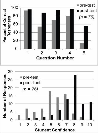
The proportion of correct responses was higher for all five questions on the post-

test, and was significantly higher at 1% level of significance for questions 2-5 (Figure 3a,

Table 1). We assume there was little gain in correct responses to question one due to its

very basic level; most students answered this question correctly on both tests and there

was little room for improvement. The lower number questions on the quiz covered

more basic concepts and the higher number questions involved higher level, critical

thinking (see supplemental material). Student gains reflect increased understanding

from the pre-test to the post-test ranging from fairly basic knowledge through critical

thinking and application, supporting the effectiveness of the activity in improving

student learning.

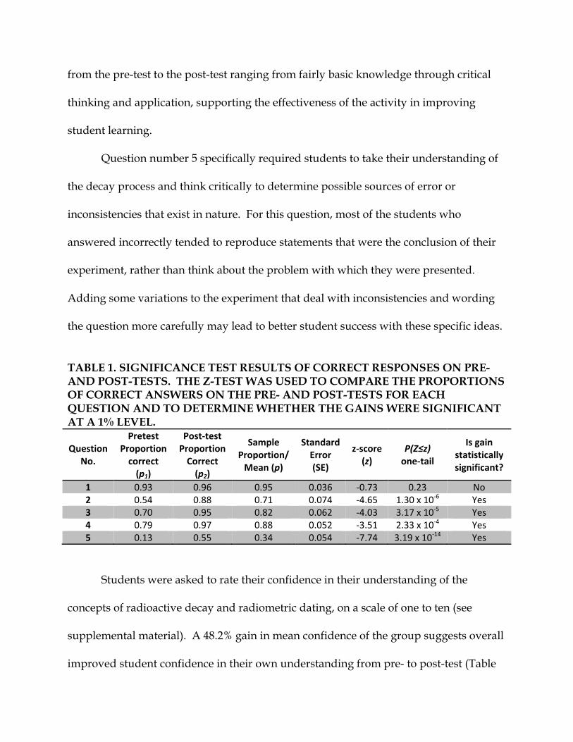
Question number 5 specifically required students to take their understanding of

the decay process and think critically to determine possible sources of error or

inconsistencies that exist in nature. For this question, most of the students who

answered incorrectly tended to reproduce statements that were the conclusion of their

experiment, rather than think about the problem with which they were presented.

Adding some variations to the experiment that deal with inconsistencies and wording

the question more carefully may lead to better student success with these specific ideas.

TABLE 1. SIGNIFICANCE TEST RESULTS OF CORRECT RESPONSES ON PRE- AND POST-TESTS. THE Z-TEST WAS USED TO COMPARE THE PROPORTIONS OF CORRECT ANSWERS ON THE PRE- AND POST-TESTS FOR EACH QUESTION AND TO DETERMINE WHETHER THE GAINS WERE SIGNIFICANT AT A 1% LEVEL.

Question No.

Pretest Proportion

correct (p1)

Post-test Proportion

Correct (p2)

Sample Proportion/

Mean (p)

Standard Error (SE)

z-score (z)

P(Z≤z) one-tail

Is gain statistically significant?

1 0.93 0.96 0.95 0.036 -0.73 0.23 No 2 0.54 0.88 0.71 0.074 -4.65 1.30 x 10-6 Yes 3 0.70 0.95 0.82 0.062 -4.03 3.17 x 10-5 Yes 4 0.79 0.97 0.88 0.052 -3.51 2.33 x 10-4 Yes 5 0.13 0.55 0.34 0.054 -7.74 3.19 x 10-14 Yes

Students were asked to rate their confidence in their understanding of the

concepts of radioactive decay and radiometric dating, on a scale of one to ten (see

supplemental material). A 48.2% gain in mean confidence of the group suggests overall

improved student confidence in their own understanding from pre- to post-test (Table

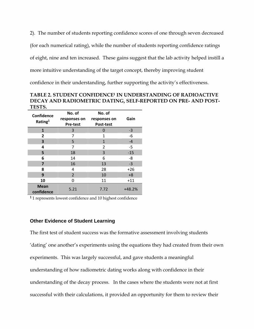
2). The number of students reporting confidence scores of one through seven decreased

(for each numerical rating), while the number of students reporting confidence ratings

of eight, nine and ten increased. These gains suggest that the lab activity helped instill a

more intuitive understanding of the target concept, thereby improving student

confidence in their understanding, further supporting the activity’s effectiveness.

TABLE 2. STUDENT CONFIDENCE1 IN UNDERSTANDING OF RADIOACTIVE DECAY AND RADIOMETRIC DATING, SELF-REPORTED ON PRE- AND POST-TESTS.

Confidence Rating1

No. of responses on

Pre-test

No. of responses on

Post-test Gain

1 3 0 -3 2 7 1 -6 3 5 1 -4 4 7 2 -5 5 18 3 -15 6 14 6 -8 7 16 13 -3 8 4 28 +26 9 2 10 +8

10 0 11 +11 Mean

confidence 5.21 7.72 +48.2%

1 1 represents lowest confidence and 10 highest confidence

Other Evidence of Student Learning

The first test of student success was the formative assessment involving students

‘dating’ one another’s experiments using the equations they had created from their own

experiments. This was largely successful, and gave students a meaningful

understanding of how radiometric dating works along with confidence in their

understanding of the decay process. In the cases where the students were not at first

successful with their calculations, it provided an opportunity for them to review their

work and their understanding, find mistakes or misconceptions and correct those errors

themselves before trying again and finding success.

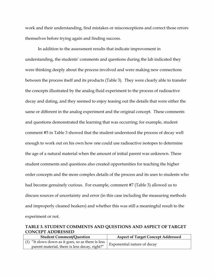
In addition to the assessment results that indicate improvement in

understanding, the students’ comments and questions during the lab indicated they

were thinking deeply about the process involved and were making new connections

between the process itself and its products (Table 3). They were clearly able to transfer

the concepts illustrated by the analog fluid experiment to the process of radioactive

decay and dating, and they seemed to enjoy teasing out the details that were either the

same or different in the analog experiment and the original concept. These comments

and questions demonstrated the learning that was occurring; for example, student

comment #5 in Table 3 showed that the student understood the process of decay well

enough to work out on his own how one could use radioactive isotopes to determine

the age of a natural material when the amount of initial parent was unknown. These

student comments and questions also created opportunities for teaching the higher

order concepts and the more complex details of the process and its uses to students who

had become genuinely curious. For example, comment #7 (Table 3) allowed us to

discuss sources of uncertainty and error (in this case including the measuring methods

and improperly cleaned beakers) and whether this was still a meaningful result to the

experiment or not.

TABLE 3. STUDENT COMMENTS AND QUESTIONS AND ASPECT OF TARGET CONCEPT ADDRESSED

Student Comment/Question Aspect of Target Concept Addressed (1) “It slows down as it goes, so as there is less

parent material, there is less decay, right?” Exponential nature of decay

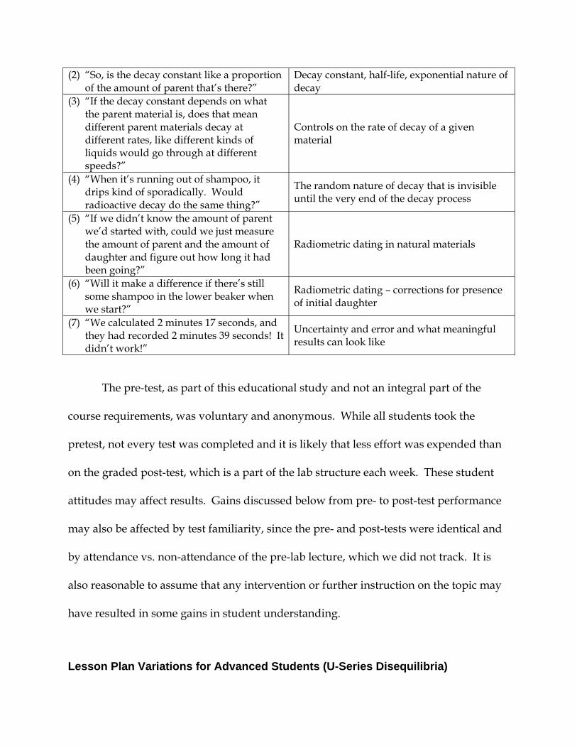
(2) “So, is the decay constant like a proportion of the amount of parent that’s there?”

Decay constant, half-life, exponential nature of decay

(3) “If the decay constant depends on what the parent material is, does that mean different parent materials decay at different rates, like different kinds of liquids would go through at different speeds?”

Controls on the rate of decay of a given material

(4) “When it’s running out of shampoo, it drips kind of sporadically. Would radioactive decay do the same thing?”

The random nature of decay that is invisible until the very end of the decay process

(5) “If we didn’t know the amount of parent we’d started with, could we just measure the amount of parent and the amount of daughter and figure out how long it had been going?”

Radiometric dating in natural materials

(6) “Will it make a difference if there’s still some shampoo in the lower beaker when we start?”

Radiometric dating – corrections for presence of initial daughter

(7) “We calculated 2 minutes 17 seconds, and they had recorded 2 minutes 39 seconds! It didn’t work!”

Uncertainty and error and what meaningful results can look like

The pre-test, as part of this educational study and not an integral part of the

course requirements, was voluntary and anonymous. While all students took the

pretest, not every test was completed and it is likely that less effort was expended than

on the graded post-test, which is a part of the lab structure each week. These student

attitudes may affect results. Gains discussed below from pre- to post-test performance

may also be affected by test familiarity, since the pre- and post-tests were identical and

by attendance vs. non-attendance of the pre-lab lecture, which we did not track. It is

also reasonable to assume that any intervention or further instruction on the topic may

have resulted in some gains in student understanding.

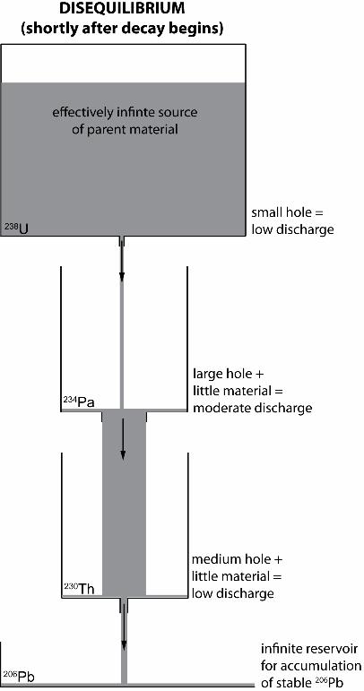
Lesson Plan Variations for Advanced Students (U-Series Disequilibria)

The activity described in this paper was inspired by attempts to explain

uranium-series disequilibria dating to advanced students (and more senior

geoscientists). Uranium-series disequilibria dating is founded on the fact that uranium

decays to form a series of radioactive daughter products that eventually decay to

produce lead, the stable daughter product (Figure 4a,b). When decay of uranium

begins in a natural substance and there are none of these intermediate products in the

material, or they are present in the ‘wrong’ proportions, the system is in

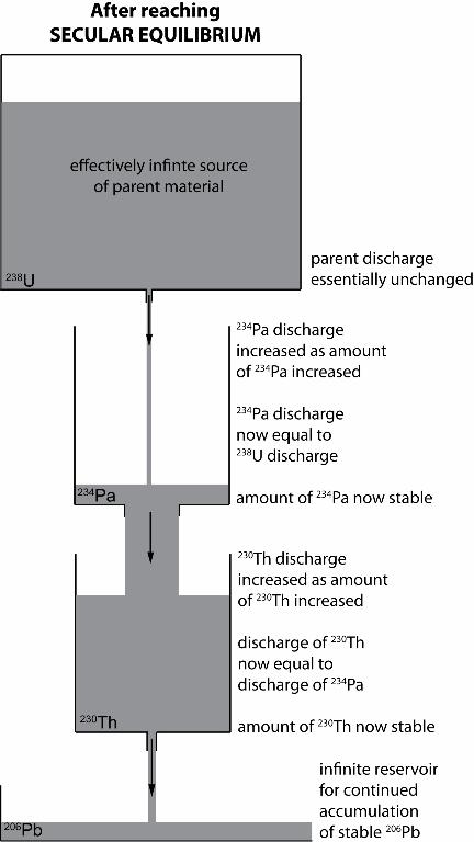
‘disequilibrium’ (Figure 4a). As decay progresses and the amount of each intermediate

radioactive isotope builds up, the system eventually reaches ‘secular equilibrium,’

where the amount of decay of the parent (known as the ‘activity’) and production of the

daughter matches the amount of decay of the daughter (its activity), and the amount of

each intermediate isotope no longer changes with time (Figure 4b). This equilibrium

state is reached when:

Where is the decay constant, N is the number of atoms, and the P and ID indicate

Parent and Intermediate Daughter, respectively. By measuring the degree of

disequilibrium, we can determine the amount of time that has passed since the material

was formed and decay began: the farther from equilibrium, the younger; the closer to

equilibrium, the older. Once the system effectively reaches secular equilibrium (ratios

of isotopes are within analytical uncertainty of matching the equation above), the

relative amounts of each isotope remain constant, it is impossible to determine the

amount of time that has passed and the intermediate U-series isotopes are no longer

useful in dating.

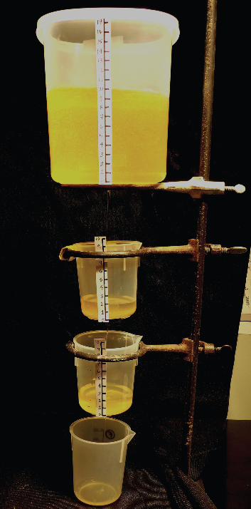
To teach the U-series decay process and disequilibria dating, we use a similar

apparatus and the same principles as the basic lesson described previously, but with

multiple beakers with various sized holes suspended in a column (Figure 4c). The

uppermost beaker should have the largest hole, but otherwise, the relative sizes of these

holes do not matter, as long as they are significantly different. The top beaker

represents the initial parent and should contain a sufficiently large amount of fluid that

the flow does not slow down significantly during the experiment. The bottom beaker

represents the final, stable daughter product, with beakers in between representing the

intermediate, unstable daughter/parent products in the decay process. The flow of

shampoo from any given upper beaker to lower beaker behaves identically to the

previously described experiment, controlled by the size of the hole and the pressure

exerted by the column of fluid. In this case, however, the experimenter can initiate the

experiment in disequilibrium (‘wrong’ levels of shampoo – empty intermediate beakers

is easiest) and observe it as it approaches equilibrium. After some time passes, if the

mass of shampoo in the uppermost beaker (‘U’) is large enough that the level doesn’t

change much during the experiment, the entire system reaches equilibrium, where the

amount being added from above to each ‘intermediate’ beaker in the series is identical

to the amount being lost out its base. Thus, the heights of fluid in the intermediate

beakers stabilize at a level that is inversely proportional to the area of the hole in its

base (its ‘decay constant’), mimicking the U-series system reaching secular equilibrium.

If you choose to assign specific elements to specific beakers, using appropriate relative

sizes of holes (larger holes for elements with larger decay constants, and vice versa) will

ensure the appropriateness of the analog.

Conclusions

Teaching using analogs enhances student understanding of difficult, non-

intuitive, unfamiliar concepts by relating them to more intuitive, familiar concepts, if

the analog is sufficiently similar to the target concept. Rate of loss of a fluid from a

beaker by flow from a hole in its base (a process that is intuitive to students) is

mathematically identical to the process by which radioactive isotopes decay. The lab

activity described herein allows students to take advantage of the structural similarities

of these two processes by studying and manipulating familiar and easily understood

hydrodynamic principles and processes and relating them to the less accessible

principles and processes of radioactive decay. This activity instills in students a much

deeper, more intuitive understanding of the concepts involved in radioactive decay and

radiometric dating than lectures and demonstrations can achieve, resulting in their

ability to make predictions regarding complications to the process and to apply this

understanding to radiometric dating activities. The results of this study illustrate the

effectiveness of this analog activity as a powerful teaching tool for an important, but

very difficult and often misunderstood concept integral to many basic sciences. Along

with improved conceptual understanding, the activity provides observational and

mathematical confidence to students, with the potential to carry over into other

challenges and enhance their confidence and success across disciplines and outside of

academia.

Acknowledgements This activity was designed and tested during a Teaching as Research project funded by

the National Science Foundation sponsored Center for the Integration of Teaching and

Learning and guided by Derek Bruff at the Vanderbilt University Center for Teaching,

who also advised us on the statistical analysis. Thanks to Drs. Molly Miller and

Brendan Bream for allowing me access to their classroom and lab sections for this study,

for giving the lecture on radioactive decay students attended before the lab, and for

sharing their syllabus materials, including learning goals, that allowed me to create the

most appropriate lesson possible. Thanks to the other Vanderbilt Teaching as Research

Fellows for guidance and support during this project, to the teaching assistants and

students in Dynamic Earth 111 who participated so enthusiastically in the study.

Thanks to David Furbish, Vanderbilt University earth fluid physicist, who detailed the

mathematical similarity of the fluid flow and radioactive decay for us. Research funded

by National Science Foundation grant EAR0635922 inspired this work and supported

the authors while it was undertaken.

References Anderson, L.W., and Krathwohl, D.R., 2001, A taxonomy for learning, teaching, and assessing: A revision of Bloom’s taxonomy of educational objectives. New York: Addison Wesley Longman. Bourdon, B., Turner, S., Henderson, G.M., and Lundstrom, C.C., 2003, Introduction to U-Series geochemistry. In Bourdon, B., Henderson., G.M., Lundstrom, C.C., and

Turner, S.P. (Eds.), Reviews in Mineralogy and Geochemistry, v. 52: Uranium-Series geochemistry: Washington DC, The Mineralogical Society, p. 1-21. Clinikier, L.M., 1980, Teaching principles of radioactive dating and population growth without calculus: American Journal of Physics, v. 48, p. 211-213. Duit, R., 1991, On the role of analogies and metaphors in learning science: Science Education, v. 75(6), p. 649-672. Dupin, J.J. and Joshua, S., 1989, Analogies and “modeling analogies” in teaching: some examples in basic electricity: Science Education, v. 73(2), p. 207-224. Evans, G.R., 1974, Radioactive decay chains – an electronic analogue: Physics Education, v. 9, p. 487-489. Faure, G. and Mensing, T.M., 2005, Isotopes: Principles and Applications, 3rd edition: New Jersey, John Wiley & Sons, 897 p. Jee, B.D., Uttal, D.H., gentner, D., Manduca, C., Shipley, T.F., Tikoff, B., Ormand, C.J., and Sageman, B., 2010, Commentary: Analogical thinking in geoscience education: Journal of Geoscience Education, c. 58(1), p. 2-13. Glynn, S.M., 1991, Explaining science concepts: A teaching-with-analogies model. In Glynn, S., Yeany, R., andBritton, B. (Eds.), The psychology of learning science: New Jersey, Erlbaum, p. 219-240. Harrison, A.G. and Treagust, D.F., 1993, Teaching with analogies: a case study in grade-10 optics: Journal of Research in Science Teaching, v. 30(10), p. 1291-1307. Jesse, K.E., 2003, Computer simulation of radioactive decay: The Physics Teacher, v. 41, p. 542-543. Kowalski, L., 1981, Simulating radioactive decay with dice: The physics teacher, v. 19, p. 113. McGeachy, F., 1988, Radioactive decay – an analog: The Physics Teacher, v. 26, p. 28-29. Orgill, M.K. and Bodnar, G.M., 2006, An Analysis of the effectiveness of analogy used in college-level biochemistry textbooks: Journal of Research in Science Teaching, v. 43, p. 1040-1060. Prather, E., 2005, Students’ beliefs about the role of atoms in radioactive decay and half-life: Journal of Geoscience Education, v. 53, p. 345-354.

Sibley, D.F., 2009, A cognitive framework for reasoning with scientific models: Journal of geoscience education, v. 57(4), p. 255-263. Thagard, P., 1992, Analogy, explanation, and education: Journal of Research in Science Teaching, v. 29, p. 537-544. White, B.Y. and Frederiksen, J.R., 1998, Inquiry, modeling and metacognition: Cognition and Instruction, v. 16, p. 3-118. Wise, D.U., 1990, Using melting ice to teach radiometric dating: Journal of Geological Education, v. 38, p. 38-40. Wunderlich, F.J. and Peastrel, M., 1978, Electronic analog of radioactive decay: American Journal of Physics, v. 46, p. 189-190.

Figure Captions

Figure 1: (a) left Schematic of buckets representing radioactive decay of the parent uranium (fluid in the upper bucket) to the daughter thorium (fluid in the lower bucket), modified from Bourdon et al., 2003. (b) right photo of apparatus set up for radioactive decay lesson.

Figure 2: (a) top Shampoo depth vs. time, illustrating exponential nature of the fluid flow. The arrows indicate the apparent half-life of the fluid, 1.5 minutes. (b) bottom Number of parent atoms (N) vs. time for 238U using a decay constant of 1.55 x 10-10y-1 (Faure and Mensing, 2005), illustrating exponential nature of decay. The arrows indicate the half-life of 238U, 4.468 billion years (Faure and Mensing, 2005).

Figure 3: (a) Student performance on the pretest vs. post-test reported as number of correct responses. (b) Self-reported student confidence on the pretest vs. post-test.

Figure 4a: Schematic illustrating U-series decay as a set of buckets, with the system out of secular equilibrium, modified from Bourdon et al., 2003.

Figure 4b: Schematic illustrating U-series decay as a set of buckets, with the system in secular equilibrium, modified from Bourdon et al., 2003.

Figure 4c: Photo of apparatus set up for U-Series decay lesson.