SMMU ECONOMICS & STTAAATISTICS WORKING PAPER SERIES SSMUU EECCOONNOOMMIICCSS && SST TTIIWWOORRKKIINNGG PPAAPPEERR SSEERRIIEESS

SSTTIICCSS

Tax Cuts, Employment and Asset Prices: A Real Intertemporal Model

Hian Teck Hoon Edmund S. Phelps

November 2002

Paper No. 23-2002 ANY OPINIONS EXPRESSED ARE THOSE OF THE AUTHOR(S) AND NOT NECESSARILY THOSE OF

THE SCHOOL OF ECONOMICS & SOCIAL SCIENCES, SMU

Tax Cuts, Employment and Asset Prices: A

Real Intertemporal Model

Hian Teck Hoon and Edmund S. Phelps∗

Singapore Management University and Columbia University

November 2002

Abstract

We determine the effects of a delayed or immediate tax cut with

or without a “sunset” feature in a real customer-market, nonRicar-

dian economy. Our model incorporates both the supply-sider channel,

through which reduced wage income taxes stimulate work effort, as

well as the Feldstein-Rubin-Summers channel, through which cuts in

income tax, in widening the deficit and thus driving up future short

real interest rates, has a chilling effect on present and future invest-

ment, so reducing growth and employment on that account. After

establishing conditions under which fiscal policy is sustainable, we

first show that a delayed tax cut may depress both the real asset price

and employment in the period running up to the implementation of

the tax cut; so this paradox is not restricted to Keynesian or other

monetary models. Second, the same ambiguity may result even if the

∗Correspondence Address: Professor Edmund S. Phelps, Department of Economics,Columbia University, International Affairs Building, Room 1004, New York, NY 10027;tel: 1(212)-854-2060; e-mail: esp2@columbia.edu

1

tax cut takes effect immediately. Third, the presence of the para-

doxical result of employment contraction does not work through nor

imply an immediate increase of the long real interest rate, contrary to

financial commentators. Fourth, in the sunset case, the post-sunset

period is characterized unambiguously by depressed asset prices and

decreased employment before recovering to their original levels. Fi-

nally, we point out that a similar analysis applies to the huge pension

problem burdening several continental European economies. So part

of their high unemployment of late may be ascribed to their loom-

ing pension outlays. We conclude, with further argumentation, that

a theory of dynamic markup variation is needed, on top of changes

in marginal tax rates, to quantitatively account for labor-leisure dis-

tortions in the U.S. at medium-term frequencies. Models hamstrung

by pure competition in frictionless markets cannot perform as well as

required. (JEL: E24, E43, E62, F41)

An anti-cyclical policy of regulating tax rates to moderate swings in economic

activity, once advanced by Keynesians and supply-siders alike (Abba Lerner,

1946; Robert Mundell, 1971), faces objections going beyond fine tuning. A

familiar drawback is that a tax-rate cut, in widening the budgetary deficit

(or reducing the surplus) jeopardizes other goals, such as national wealth

accumulation and thus economic growth. A decisive objection, if sustained,

is that, by raising long-term interest rates and real exchange rates, thus cur-

tailing domestic investment and driving customers abroad, a tax cut operates

perversely to contract employment—at least early on, precisely when the aim

is an employment boost. The same objections apply to the claims made in

the present debate over secular fiscal policy. Those who would dispose of

looming budgetary surpluses by the occasional tax cut lest public spending

go on rising in relative terms claim it will have the beneficial side effect of

boosting employment. Those who would instead hold tax rates steady and

wipe out surpluses with the occasional new public program appear to believe

2

that their approach would also be a boon to employment—at least not a

drag. But these objections have not been developed very far.

The first argument against the supposition that a cut in tax rates is

expansionary for employment, at least initially, is that by Olivier Blanchard

(1981). He takes up the effect of an “anticipated” fiscal expansion—one that

is announced at t0 and to be implemented at subsequent t1. Such a premise

does not accurately describe tax cuts legislated promptly in response to an

emergency but it does seem to fit very well the more structural kind of tax cut

enacted in the U.S. in the summer of 2001. (This bill, the Economic Growth

and Tax Relief Reconciliation Act (EGTRRA), schedules the largest rate

reductions in the years from about 2005 to 2010, with a “sunset” for these

cuts scheduled for 2011.) Constructing a dynamized version of the Keynesian

closed-economy model, Blanchard shows that in the “bad news” case—and

only in that case—the sudden expectation of the future stimulus drives up

the long rate of interest and causes asset prices to drop correspondingly, with

the result that investment expenditure and output contract in the first phase

of the scenario. However, it would be anomalous to use a model lacking a

natural, or structural, path of unemployment to analyze the effects of a tax

cut reaching full strength some 9 years in the future, like the recent Bush

tax cut, or even 3 years, such as the first Reagan tax cut. We would not

know whether, in a model with a natural rate path, an initial fall of output

might be accompanied by a rise of the natural output path, which would

put a different complexion on the first result. Therefore, when the interval of

study may run for a decade, a model of the effects on the natural rate path

is required. Furthermore, a non-monetary perspective on the matter seems

particularly appropriate for evaluating the claims for back-loaded tax cuts

made by adherents to supply-side analysis, since a natural rate model will

incorporate some or all of the supply-sider effects.

Our analysis incorporates both the supply-sider channel, through which

3

reduced wage income taxes stimulate work effort, as well as a channel revived

by Rubin and Summers in the 90’s and earlier championed by Feldstein in

the early 80’s when he was the chairman of the Reagan Council of Economic

Advisors.1 The Feldstein-Rubin-Summers contention was that cutting rates

of income tax, in widening the deficit and thus driving up future short rates

of (real) interest, has a chilling effect on present and future investment, so

reducing growth and employment on that account. They suggested that

this countervailing effect was strong enough to make such tax cutting utterly

perverse—the lower tax rates notwithstanding. We examine this financial hy-

pothesis of a perverse effect from tax cuts in a framework in the structuralist

spirit of Edmund Phelps (1994)—hence non-monetary and inter-generational

though, for simplicity, we exclude unemployment arising from incentive wages

and use instead a variable supply of “hours” that is modeled much like the

demand for consumption.2

Our model describes a closed economy. It is not the Ricardian type of

economy favored by RBC theorists and some public finance theorists. In-

stead, we follow the treatment by Blanchard (1985) in which worker-savers

toil throughout life, save by buying annuities invested in the shares of the

firms, and die off exponentially. In order to provide a business asset to back

the shares of firms, and in order to give a role to the variation of price-

marginal cost markups in explaining the big changes in the wedge between

1For an account of Feldstein’s views, see Feldstein (1993).2See Robert Hall (1997) for an empirical effort to explain movements of employment

in terms of such a model of labor supply. Our paper makes two main departures fromthe Hall framework: We introduce a dynamic theory of variable markups, and we alsointroduce a public finance distortion as in Casey Mulligan (2002). We return to a detaileddiscussion of the behavior of the markup and the public finance distortion in understandingkey historical episodes in the U.S. in the paper’s concluding section. We argue that atheory of dynamic markup variation is needed, on top of changes in marginal tax rates, toquantitatively account for labor-leisure distortions in the U.S. at medium-term frequencies.

4

the value marginal product of labor and the marginal rate of substitution in

consumption and leisure (the “marginal value of time” measured in consump-

tion units), we use the customer-market model set up by Phelps and Sidney

Winter (1970) and placed in a general-equilibrium setting by Guillermo Calvo

and Phelps (1983).3 Owing to frictions in the transmission of price informa-

tion, the competition of firms for market share will fail to wipe out all pure

profit, and so leave the optimal price charged by firms hanging above the

average and marginal cost, provided that the current short-term real inter-

est rate is positive. Firms set mark-ups below the monopolist’s level but

above the pure competitor’s level—how high depending upon the value per

unit placed on the average and marginal customer. The output supply and

thus also employment is an increasing function of this per-unit asset value

normalized by dividing it by the exponentially rising productivity parameter

and a decreasing function of the tax rate. Aggregate investment and na-

tional saving here are always zero but we study employment and the other

variables.

This paper will study cuts in the tax rate on wage income that are imme-

diate or delayed and possess or lack a sunset feature. Of course, this focus

is inspired by the Bush tax cut, which would see income tax rates in 2011

go back to their 2000 levels. We find conditions under which fiscal policy

is sustainable—so the debt-income ratio neither explodes nor implodes—

despite a return of income tax rates, from sunset onwards, to their original

rather than higher levels or despite a permanent tax cut. (Despite the pile-

3Rotemberg and Woodford (1992) argued convincingly that a model featuring imperfectcompetition in the product market is required in order to explain how aggregate demandchanges, such as increases in government purchases, can increase output while at thesame time raise the real wage. Our paper goes further to argue that fully accounting forvariations in the wedge between the value marginal product of labor and the marginal rateof substitution in consumption and leisure requires tracking not only changes in the taxrate but also changes in the price-marginal cost markup.

5

up of public debt due to widening budget deficits as a result of income tax

cutting, we show that depressed asset prices drive down the short-term nat-

ural rate of interest thus alleviating the interest burden of debt.) We show

in that case that a delayed tax cut may depress both the real asset price

and employment in the period running up to the implementation of the tax

cut; so this paradox is not restricted to Keynesian or other monetary models,

such as Blanchard’s. Furthermore, we show that the same ambiguity may

result even if the tax cut takes effect immediately. The presence of the para-

doxical result of employment contraction does not work through nor imply

an immediate increase of the long real interest rate, contrary to financial

commentators. Finally, we show in the sunset case that the post-sunset pe-

riod is characterized unambiguously by depressed asset prices and decreased

employment before they recover to their original levels.

Our work here relates to some papers other than those already cited.

Mankiw and Summers (1986) argue on theoretical and empirical grounds

that a tax cut, in increasing households’ disposable income, could raise the

demand for money and, given an unchanged money supply, contract output in

a Keynesian model. As with our comment on the Blanchard (1981) analysis,

a full understanding of the effects of back-loaded tax cuts that kick in in

full force only towards the latter half of the decade requires a treatment of

the natural path of output and employment. Perotti (1999) examines both

theoretically and empirically how drastic cuts in government deficits—fiscal

consolidation—in countries with exceptionally high levels of the dedt-GDP

ratio could lead to consumption booms.4 His paper differs from ours in

neglecting employment responses by assuming perfectly inelastic supplies of

labor, and relies on a competitive framework. Phelps (1992) develops a

4Perotti (1999) also provides a review of the related papers on “expansionary fiscalconsolidations” but these papers do not rely on the supply-sider channels and asset pricechannels emphasized in our paper.

6

closed-economy customer market model and examines a public debt shock

but it does not incorporate the distortionary effect of the wage income tax

that plays a crucial role in this paper and it neither analyzes the effects of a

back-loaded tax cut nor studies the endogenous evolution of the debt-income

ratio in a fully specified general-equilibrium system.

The paper is organized as follows. In Section 1, we study the optimization

problems solved by individual agents and set up the basic model. In Section

2, we study the response of asset prices, real interest rates and employment to

an announced future helicopter drop of public debt. We contrast these results

to those obtained under an equivalently-sized “entitlement bomb” scenario.

Section 3 treats the debt-income ratio as an endogenous variable and uses

the full general-equilibrium system to study the economy’s response to shocks

to the wage-income tax rate. In the concluding section, we discuss the role

played by the markup and the public finance distortion in understanding

key historical episodes in the U.S. We also point out that a similar analysis

applies to the huge pension problem burdening several continental European

economies. So part of their high unemployment of late may be ascribed to

their looming pension outlays.

1. The Model

Let us consider a closed economy where investment takes place in “cus-

tomers.” There is one homogeneous good and four marketable assets—

shares, which are titles to the stream of profits, private short- and long-term

bonds issued and held by individuals, and government bonds. These non-

monetary assets are assumed to be perfect substitutes so arbitrage among

them implies that they have the same expected short-term rate of return. It

will be innocuous but convenient to suppose that all (nonhuman) wealth, in

equilibrium, is held in the form of shares and public debt. The economy is

initially in a steady-growth state, growing at the rate λ, with a nonnegative

7

public debt-to-productivity ratio (called normalized debt). A proportional

wage income tax is imposed to finance government expenditure.

Agents derive utility from consumption and leisure, have finite lives and

face an instantaneous probability of death θ that is constant throughout

life. Let c(s, t) denote consumption at time t of an agent born at time

s, l(s, t) labor supply, w(s, t) nonhuman wealth, and h(s, t) human wealth.

Also let ys(t) be government entitlement per agent and vh(t) be the real

hourly household wage (in terms of output, our numeraire good), which is

related to the hourly labor cost to the firm, vf , by vf ≡ (1+τ)vh, τ being the

proportional wage income tax rate. We let r(t) denote the real instantaneous

short-term interest rate, ρ the pure rate of time preference, and L the total

time available per worker.

The agent maximizes∫ ∞

t[log c(s, µ) + B log(L− l(s, µ))] exp−(θ+ρ)(µ−t) dµ, B > 0

subject to

dw(s, t)

dt= [r(t) + θ]w(s, t) + vh(t)l(s, t) + ys(t)− c(s, t)

and a transversality condition that prevents agents from going indefinitely

into debt. The solution to the agent’s problem is given by

c(s, t) = (θ + ρ)[h(s, t) + w(s, t)],

L− l(s, t)

c(s, t)=

B

vh(t),

where human wealth is given by

h(s, t) =∫ ∞

t[l(s, µ)vh(µ) + ys(µ)] exp−

∫ µ

t[r(k)+θ]dk dµ.

Normalizing the population (equal to labor force) to unity, dropping the

time index t and denoting aggregate variables by capital letters, we obtain

C = (θ + ρ)[H + W ],(1)

8

L− L

C=

B

vh,(2)

H = (r + θ)H − (Lvh + ys),(3)

W = rW + Lvh + ys − C,(4)

where a dot over a variable denotes its time derivative. We note from (3) and

(4) that whereas the rate of interest used to discount after-tax wage income

and entitlement is (r + θ), aggregate nonhuman wealth accumulates at rate

r. It is this difference in discount rates that results in the non-neutrality of

debt and deficits.

The government’s budget constraint can, in general, be expressed as

D = rD + G + ys − τLvh,(5)

where D is the level of government debt, G is the amount of government

purchases, ys is government entitlement, and tax revenue collected is entirely

from wage income taxation. For simplicity, we will throughout set G = 0.

Assuming that, in equilibrium, agents have zero holdings of private bonds,

W ≡ V +D, where V is the total value of shares held by individuals. Taking

the time derivative of (1), and using (3) and (4), we obtain

C = (θ + ρ)[rW + (r + θ)H − C].(6)

Using (1) in (6), we obtain, after re-arrangement of terms,

C

C= (r − ρ)− θ(θ + ρ)[V + D]

C.(7)

Next, defining C ≡ C/Λ, D ≡ D/Λ, V ≡ V/Λ, ys ≡ ys/Λ, and vh ≡vh/Λ, where Λ is the measure of Harrod-neutral productivity level, we can

transform (5) and (7) to obtain

˙D = (r − λ)D + ys − τLvh,(8)

˙C = (r − λ− ρ)C − θ(θ + ρ)[V + D].(9)

9

We can now turn to the firms. With labor as the only factor of produc-

tion, individual firms minimize costs taking wages as given. In the general

equilibrium, however, wages must adjust to equate aggregate labor demand

to aggregate labor supply. Consequently, using (2), unit cost, c ≡ vf/Λ, can

be expressed as

c =(1 + τ)B(Cs

Λ)

L− (Cs

Λ)x

,(10)

where x is the stock of customers, and the consumption demand appearing

in (2) has further been equated to the consumption supplied per customer,

Cs, since in the closed economy, the number of customers is equal to the

population, which we have set equal to the size of the labor force. Under

our normalization of the population size to one, x = 1. We can check from

(10) that the partial elasticity of unit cost with respect to Cs is greater than

one. The partial elasticity of the unit cost with respect to x is equal to

L/(L − L). (If we think of a typical eight-hour work day, this is a number

like one-half.) Note also that, ceteris paribus, an increase in the wage income

tax rate increases unit cost, while a rise in the Harrod-neutral productivity

parameter decreases unit cost. We express the unit cost in reduced form as

c = Υ(Cs, x; τ, Λ); ΥCs > 0, Υx > 0, Υτ > 0, ΥΛ < 0.

The firm has to choose the price at which to sell to its current cus-

tomers. Raising its price causes a decrease, and lowering the price an in-

crease, in the quantity demanded by its current customers according to a

per-customer demand relationship, D(pi/p, Cs). For simplicity, we assume

that D(·) is homogeneous of degree one in total sales, Cs, and so we write

Csi = η(pi/p)Cs; η′(pi/p) < 0; η(1) = 1. Each firm chooses the path of its

real price or, equivalently, the path of its supply per customer to its con-

sumers, to maximize the present discounted value of its cash flows. The

maximum at the ith firm is the value of the firm, V i, which depends upon

10

xi:

V i0 ≡ max

∫ ∞

0

[(pi

t

pt

)−Υ(Cst , xt; τ, Λt)

]η(

pit

pt

)Cst x

it exp−

∫ t

0rsds dt.

The maximization is subject to the differential equation giving the motion

of the stock of customers of the ith firm as a function of its relative, or real,

price given by (11) below and an initial xi0:

xi = g(pi

p)xi; g′ < 0, g′′ ≤ 0; g(1) = 0.(11)

The first-order condition for optimal pi is

η(pi

p)Csxi

p+

[(pi

p)−Υ(Cs, x; τ, Λ)

]η′(

pi

p)Csxi

p+ qi

mg′(pi

p)xi

p= 0,(12)

where qim is the shadow price, or worth, of an additional customer. Another

two other necessary first-order conditions (which are also sufficient under our

assumptions) from solving the optimal control problem are:

qim = [r − g(

pi

p)]qi

m −[(pi

p)−Υ(Cs, x; τ, Λ)

]η(

pi

p)Cs,(13)

limt→∞ exp−

∫ t

0rsds qi

mtxit = 0.(14)

We note that “marginal q” denoted qim is equal to “average q,” which we

denote as qia ≡ V i/xi, so qi

m = qia = qi.5

Equating pi to p, and setting qi = q, delivers the condition on consumer-

good supply per firm for product-market equilibrium:[1 +

η(1)

η′(1)−Υ(Cs, x; τ, Λ)

]= −(

q

Cs)

(g′(1)

η′(1)

); η(1) = 1.(15)

5The proof is as follows: Taking the time derivative of the product qimtx

it,

we obtain d(qimtx

it)/dt = qi

mt[dxit/dt] + xi

t[dqimt/dt] = rtq

imtx

it − [(pi

t/pt) −Υ(Cs

t , xt; τ, Λt)]η(pit/pt)Cs

t xit, after using (11) and (13). Integrating, and using (14), we

obtain qimtx

it =

∫∞t

[(pik/pk)−Υ(Cs

k, xk; τ, Λk)]η(pik/pk)Cs

kxik exp−

∫ k

trsds

dk ≡ V it .

11

The expression in the square brackets is the algebraic excess of marginal

revenue over marginal cost, a negative value in customer-market models as

the firm supplies more than called for by the static monopolist’s formula for

maximum current profit, giving up some of the maximum current profit for

the sake of its longer-term interests. An increase in q means that profits from

future customers are high so that each firm reduces its price ( equivalently its

markup) in order to increase its customer base. To handle economic growth,

it is useful to note from (10) that we can express unit cost as c = Υ(Cs, x; τ),

where Cs ≡ Cs/Λ, so (15) can be transformed to

[1 +

η(1)

η′(1)−Υ(Cs, x; τ)

]= −(

q

Cs)

(g′(1)

η′(1)

); η(1) = 1,(16)

where q ≡ q/Λ is normalized Q.

From (16), we can express normalized consumer-good supply per cus-

tomer, Cs, which equals employment, L, in terms of q, x, and τ , that

is, Cs = L = Ω(q, x; τ). It is straightforward to show that 0 < eq ≡d ln Cs/d ln q < 1, and − 1 < ex ≡ d ln Cs/d ln x < 0, where ej denotes

the partial elasticity of Cs with respect to the variable j. Also, Ωτ < 0. An

increase in q makes investment in customers through reducing the markup

attractive and so expands current output and employment. With rising

marginal cost, an increase in the number of customers at each firm leads

to a less than proportionate decline in the amount of (normalized) output

supplied per customer.6 An increase in wage income tax contracts each

firm’s supply. Writing q ≡ q/Cs ≡ q/Cs, we also note that the markup,

m ≡ c−1, is a unique decreasing function of q. We express this relationship

as: m ≡ c−1 = φ(q); φ′(q) < 0. An increase in investment in customers

through lowering current markups is attractive when the present discounted

value of the future returns from investment (q) are high relative to its cost,

6We use the condition that the partial elasticity of the unit cost with respect to x isequal to L/(L− L), a number typically less than one.

12

which depends on the current level of sales (C).

In a symmetric situation across firms, (13) simplifies to

[1−Υ(Ω(q, 1; τ), 1; τ)]Ω(q, 1; τ)

q+

˙q

q+ λ + g(1) = r; g(1) = 0,(17)

after using x = 1 and Cs = Ω(q, x; τ). Equation (17) in the firm’s instanta-

neous rate of return to investment in its stock of assets, which are customers,

is an inter-temporal condition of capital-market equilibrium: it is entailed by

correct expectations of ˙q and r at all future dates. It can be seen from the

unit cost function, Υ(· · ·), in (17) that, given q and x = 1, a decrease in τ

lowers the unit cost directly, and increases it indirectly through raising Cs.

Using Cs = Ω(q, x; τ) in (16), however, shows that the direct effect domi-

nates so, given q, a decrease in τ unambiguously lowers unit cost. In other

words, given that the elasticity of (normalized) output supplied per customer

with respect to q is less than one, ceteris paribus, an increase in q lowers the

markup while a decrease in τ increases the markup. An alternative way of

expressing the markup function will be useful: m ≡ c−1 = ψ(q; τ); ψq < 0

and ψτ < 0.

Equating consumption demand to consumption supply in (9), and noting

V ≡ qx, we obtain an expression for r:

r = λ + ρ +θ(θ + ρ)(q + D)

Ω(q, 1; τ)+ eq

(˙q

q

); 0 < eq < 1,(18)

where we have used x = 1. (If we define the long-term (real) interest rate

as the yield on consols paying a constant coupon flow of unity, and let R be

their yield and hence R−1 be their price, arbitrage between short and long

bonds gives the condition R = r + (R/R).) Substituting (18) into (17), and

noting that g(1) = 0, we obtain

[1− eq]˙q

q= ρ +

θ(θ + ρ)(q + D)

Ω(q, 1; τ)

− [1−Υ(Ω(q, 1; τ), 1; τ)]Ω(q, 1; τ)

q.(19)

13

It is clear that the full-fledged model makes both q and D endogenous

variables. Before we study the full-fledged model, however, it will be useful,

for purposes of developing intuition, to study (19) treating normalized debt,

D, first as a parameter. We proceed with our analysis in this order in the

next two sections.

2. The Analysis Treating Normalized Debt as a Parameter

A. The Debt Bomb Scenario

Suppose that we start off in an initial equilibrium where D = 0, ys = 0,

and τ = 0. Then, we have the following lemma:

LEMMA 1: With D = 0, ys = 0, and τ = 0, the rational expectations

equilibrium is given by a unique value of q that makes the righthand side of

(19) equal to zero.

Since the elasticity of Cs with respect to q is less than one, the righthand

side (RHS) of (19) is increasing in q. Applying the transversality condition,

limt→∞[exp−∫ t

0(rs−λ)ds qtxt] = 0, the unique perfect foresight path of q requires

that it be stationary at the value that makes ˙q = 0.

Let us now suppose that at t0, it is announced that at t1, there will be

a helicopter drop of public debt, ∆ > 0, which will be financed by raising

wage income taxes to cover interest payments on the new constant level of

(normalized) public debt after t1 so that τLvh = (r − λ)∆. To analyze the

effects on asset prices, interest rates, and employment, it is convenient to refer

to the first panel of Figure 1. Initially, q is equal to qA. Working backwards,

let us ask, “What is the value of q in the new stationary state?” (Note that

given the instability of the system, the new stationary state must be attained

precisely at t1.) As we noted above, the unit cost, c ≡ Υ(· · ·), is a monotone

14

increasing function of q/Cs. Substituting that relation into (17), noting

that g(1) = 0, and setting ˙q = 0, we obtain a negatively-sloping relationship

relating the LHS of (17) to q/Cs (see Figure 2). Next, turning to (18), setting

˙q = 0 and letting D = 0 initially, gives a positively-sloping relationship

relating the RHS of (18) to q/Cs. Now with D = ∆ > 0, the positively-

sloping relationship shifts upwards, hence leftwards. The result is that the

value of q/Cs corresponding to the intersection declines. Consequently, the

equilibrium markup is increased, and labor demand is decreased on that

account, at t1.

We have just shown that q/Cs ≡ q/Ω(q, 1, τ) must fall at t1.7 Given q,

an increase in τ reduces Cs, which would raise q/Cs. Since the elasticity

of Cs with respect to q is between zero and one, it must be that q falls by

more than proportionately to achieve the implied drop in q/Cs. The new

schedule in Figure 1 relating ˙q/q to q must, therefore, be to the left of the

old schedule. As there can only be one initial jump in q at the moment the

announcement is made, i.e. at t0, and the economy must be at the value

of q that makes ˙q = 0 at t1 (namely, at qC in Figure 1), the path taken by

the economy after the initial jump is given by BC along the old schedule

in Figure 1. Upon receiving the announcement of future fiscal expansion,

therefore, asset prices fall immediately from qA to qB, and the expected rate

of change of q, i.e., the expected capital gains term, goes from zero to a

negative value as market participants form a rational expectation of further

asset price declines. In fact, asset prices continue to decline at an increasing

rate until t1 when ˙q jumps up from a negative value (on the old schedule) to

zero (on the new schedule). The stock market value cannot jump at the time

of implementation, t1, to avoid the possibility of making anticipated infinite

7The value of τ that must be raised to finance the interest on debt is given implicitlyby the following equation: τ(1+τ)−1Υ(Ω(qC , 1; τ), 1; τ)Ω(qC , 1; τ) = [λ+ρ+θ(θ+ρ)(qC +∆)(Ω(qC , 1; τ))−1]∆, where qC is the stock market value attained at t1 and shown in Figure1.

15

rates of capital gain or loss. The implied paths taken by the current short-

term real interest rate and employment, which equals normalized output, are

given in the following proposition:

PROPOSITION I: At t0, the short-term real interest rate drops, and it con-

tinues to fall steadily between t0 and t1. Then at t1, it jumps up permanently

to a level higher than the original level. Employment, which equals normal-

ized output, drops at t0, and continues its decline to reach a permanently

lower level at t1.8

To understand how asset prices affect the natural rate of interest, it is

useful to develop an analytical framework that is very close in spirit to that

used by Lloyd Metzler (1951) in his classic article, “Wealth, saving, and the

rate of interest.” In that paper, Metzler developed a diagram in the (wealth,

interest rate) plane (his Figure 1, p. 101), consisting of an upward-sloping

WW schedule and a downward-sloping AA schedule. The WW schedule,

which Metzler called the wealth-requirements schedule, gives the combina-

tions of the interest rate and the real value of private wealth that would make

“the community’s demand for goods and services as a whole equal [to] its

capacity to produce.” (p. 101) The reasoning underlying his AA schedule

is the following: “In the short run the income earned by the common stock

is a given amount, determined by the fixed supplies of the various agents

of production; and this means that the yield, or the rate of interest, varies

inversely with the real value of the stock.” (p. 101)

We develop in Figure 3 the Metzler diagram in our non-monetary model.

The upward-sloping schedule, WW , gives the amounts of (normalized) pri-

8Notice from the third panel in Figure 1 that there is a further discontinuous drop innormalized output, and hence employment, at t1. This is because q does not jump att1 but wage income tax is increased at that point to finance the interest on debt. Thenegative supply-siders’ effect leads to the further decline in employment at t1.

16

vate wealth required, at different interest rates and at given ˙q/q, to make

aggregate demand (here, simply Cd) equal to aggregate supply, Cs, that is,

to attain product-market equilibrium. Since the condition that consumption

demand equals consumption supply, Cd = Cs, holds at each moment, it is

also true that ˙Cd

t = ˙Cs

t for all t. Moreover, since Cs = Ω(q, 1; τ), we can write˙C

s

= eq[ ˙q/q]Ω(q, 1; τ). From (18), we can express the wealth-requirements

condition as:

W =

[(r − λ− ρ)− eq

(˙q

q

)]Ω(q, 1; τ)

θ(θ + ρ).(20)

We note that, initially with τ = 0 and D = 0, W ≡ q since x = 1. We can,

therefore, re-express (20) as:

θ(θ + ρ)

[q

Ω(q, 1; τ)

]= (r − λ− ρ)− eq

(˙q

q

),

from which, since the elasticity of Cs with respect to q is less than one, we

have, for given ˙q/q, a positive relationship between r and q. In Figure 3, the

WW schedule drawn in bold is the initial schedule with τ = 0, D = 0 and

˙q/q = 0. The AA schedule, which we can call the assets-market equilibrium

locus, is given in our non-monetary model by (17), which we rewrite here as:

r = λ +[1−Υ(Ω(q, 1; τ), 1; τ)]Ω(q, 1; τ)

q+

˙q

q.(21)

Since the elasticity of Cs with respect to q is less than one, we have, for

given ˙q/q, a negative relationship between r and q. The AA schedule drawn

in bold is the initial schedule with τ = 0, D = 0 and ˙q/q = 0.

The initial equilibrium corresponds to point 1 in Figure 3, with q equal

to the corresponding qA in Figure 1. The sudden announcement at t0 of a

helicopter drop of public debt at t1 causes current r to fall for the following

reason: The expectation of capital loss on the holding of the common stock

requires that current share price, q, falls in order to bring the total rate of

17

return to holding a share equal to what it was before. Hence, there is a

leftward shift of the AA schedule. The expectation of a capital loss implies

that there is an expectation of a decline in output supplied as well since firms

will be expected to raise their markups on account of the expected fall in q.

This serves to raise the wealth requirement for product-market equilibrium,

implying a rightward shift of the WW schedule. The short rate, therefore,

unambiguously falls (see Figure 3). Moreover, the expectation of capital loss

necessarily reduces the equilibrium value of current q. To see this, notice

that at a given level of q, say at qA, a one percentage point decline of ˙q/q

requires that r falls by eq percent to satisfy the product-market equilibrium

condition, so the WW schedule shifts down by 0 < eq < 1 percent. To

satisfy assets-market equilibrium, however, requires that r falls by exactly

one percent. Since the AA schedule shifts down by more than the WW

schedule, the fall in r corresponding to the movement from point 1 to point

2 in Figure 3 involves a fall of q from qA to qB.

As the rate of expected capital loss further rises between t0 and t1 (see

the first panel of Figure 1), both the WW and AA schedules continue to

shift down, with the latter curve shifting by more than the former, thereby

generating further declines in r and q. At t1, with ˙q/q going from a negative

value to zero, the AA schedule shifts back to its original position (the bold

line). The wealth-requirements schedule, however, does not go back to its

original position, as wealth now includes also the holding of public debt,

∆ > 0. A horizontal wedge, of size ∆ > 0, is now driven between the AA

and WW schedules with the consequence that the short rate at t1 onwards

(corresponding to point 3 in Figure 3) is above the original short rate. We

plot the time path of r in the second panel of Figure 1, where we see that the

short-term real interest rate first drops at t0 and continues a path of steady

decline between t0 and t1 before it jumps up to a plateau that is higher than

the level attained before the shock.

18

The path of normalized output, hence employment, can be inferred from

the output supply function, Cs = Ω(q, 1; τ). Since q drops at t0 and continues

its decline until t1, industry markups first increase and continue to increase

further until t1. As a result, employment first contracts and continues to

decline until t1. At t1, although q does not jump, the imposition of the

wage income tax causes a further contraction in normalized output. Hence

employment, though falling steadily since t0 as asset prices steadily decline,

suffers a discontinuous drop at t1 due to the supply-sider effect of higher wage

income taxes imposed at that time.

It is worth pointing out that since the short rate, r, initially drops and

continues to fall (until t1) in response to the news of a future helicopter drop

of public debt, the depressed stock market could be accompanied by an initial

decline in the long rate, R. Recall that arbitrage ensures R = r + (R/R). If

the term structure is downward sloping at announcement, R unambiguously

falls below r since R/R < 0. We depict an illustrative path (dotted line) in

the second panel in Figure 1 denoted RI . If the term structure is upward

sloping at announcement so R/R > 0, it is still possible that R initially drops

if r falls by more than the rate of capital loss on holding a long bond, where

R−1 is the price of the long-term bond. We depict another illustrative path

(broken line) in the second panel in Figure 1 denoted RII . Hence observing

an initial fall in the long rate is not prima facie evidence against the Feldstein-

Rubin-Summers channel, going from prospective debt to higher future short

rates and a decline in asset prices and employment, contrary to financial

commentators.9

Intuitively, the slump in the stock market that follows the announcement

of future fiscal expansion can be explained as follows: A lower value of equity

in the future is required to make the rate of return in equity investment

9See the editorial entitled, “The Demise of Rubinomics,” in the Wall Street Journal(August 28, 2002).

19

equal to the higher short rate in the future. Under rational expectation,

this anticipation drives down equity prices today. The current drop in stock

market value reduces nonhuman wealth, which reduces current consumption

demand, and puts downward pressure on the current short rate. Despite

lower short rates, and notwithstanding lower long rates, economic activity is

not stimulated since the decline in stock market reflects the reduced worth of

a future customer and that is decisive in driving firms to raise their current

markups. Current output and employment are, therefore, depressed.10

The expectation of the higher short rate from t1 onwards is, however, only

one channel causing the slump in asset prices. Since the debt bomb explosion

occurring at t1 has the effect thereafter of requiring an increase of tax rates

to re-balance the budget, now swollen by the increased debt burden, the vf

curve, hence the cost curve, is pushed up with the result that quasi-rent is

reduced beginning at t1. The anticipation of this reduced level of aggregate

quasi-rents on the customer stock is another factor causing an immediate

drop in the stock market at t0.11

10We have demonstrated theoretically that the decline in asset prices coincides withan initial decline in the short-term natural rate of interest. Is this relationship observedempirically? Do we tend to see, say, in the past fifteen years, a decline in the stock marketbeing associated with a decline in the short-term real interest rate, and a booming stockmarket associated with an increase in the short-term real interest rate. We suggest thatthe answer is in the affirmative. A number of authors who have examined the behaviorof the Federal Reserve System since the mid-eighties onwards have argued that implicitinflation targeting by the Fed has involved raising the short-term real interest rate as ameans of dampening aggregate demand when asset prices increased (see Ben Bernankeand Mark Gertler, 1999; Richard Clarida, Jordi Gali and Gertler, 2000). When stockprices declined in 2001, the Fed lowered the short-term real interest rate in a series of cutsto stimulate aggregate demand.

11Mundell (1960) showed that when the corporate income tax is raised to finance intereston debt, the capitalization of the tax, hence a drop of the current real asset price, acts toreduce wealth even as increased private holding of public debt increases wealth. He pointedout that the Metzler (1951) analysis regarding public debt failed to take into account this

20

B. The Entitlement Bomb Scenario

Republicans may complain that the Democrats’ alternative to the debt

bomb, a rain of increased entitlement spending, which in our stylized model

also commences in the medium-future, has the same effect. They are right

up to a point: The increased spending, in requiring thereafter an increase

of tax rates for budget balance, also reduces quasi-rents and as a result the

stock market also drops in anticipation of that. (In fact, the Republicans

would justify their debt bomb as a second-best move serving to ward off the

worse outcome of increased entitlements.)

The economics is more complicated, however, since the debt bomb im-

pacts on the stock market and hence investment and employment through a

second channel—higher expected future short rates from t1 onwards—which

the rain of entitlements does not. With the Blanchard-Yaari demographics,

the debt bomb is converted to an annuity by individuals so that in expected

value sense the whole stream of interest in perpetuity is expected to be con-

sumed. So there is a bigger stimulus to consumption than that imparted by

an equal-sized “entitlement bomb” in our non-Ricardian setup.12 (There is

offsetting capitalization effect. Metzler (1973) objected that corporate taxes were not asubstantial part of total taxes collected in the U.S. Our analysis, however, shows that theasset market also capitalizes the effects of higher expected wage income taxes required tofinance the interest on debt.

12Suppose that the government announces that it will introduce a steady stream of wel-fare entitlements at t1 onwards such that ys = (rD

1 −λ)∆, where rD1 is the short rate that

prevails from t1 onwards in the debt bomb scenario. Human wealth at t0 is not changed

by the welfare entitlement program and is given simply by∫∞

t0vf

t Lt exp−

∫ µ

t0(rk−λ+θ)dk

dµ

since what the government gives in quasi-human wealth, viz. the entitlement bene-fit (the normalized entitlement’s value doesn’t grow at r(t) − λ, but at r(t) − λ + θ),is taken away in taxes on labor. The human wealth under the debt bomb scenario,however, has an additional term, which disappears only under Ricardian Equivalence:

Ht0 =∫∞

t0vf

t Lt exp−

∫ µ

t0(rk−λ+θ)dk

dµ+[ θys

(rD1 −λ)(rD

1 −λ+θ)] exp

−∫ t1

t0(rk−λ+θ)dk

. Therefore, in

21

also a larger implied rise in demand for leisure under the debt bomb scenario.

Using (2), and noting that vh ≡ (1 + τ)−1vf and m ≡ c−1 = (vf/Λ)−1, we

have (L − L)/C = B(1 + τ)m. The greater stimulus to consumption, C,

carries with it a greater increase in demand for leisure, given the terms on

the righthand side. Additionally, there is a greater increase in the current

markup as well, so there is also a larger increase in the demand for leisure

relative to consumption under the debt bomb scenario.) Consequently, from

t1 onwards, the short rate path corresponding to the debt bomb scenario

lies everywhere above the short rate path corresponding to the entitlement

bomb scenario. (Under the entitlement bomb scenario, the short rate from

t1 onwards is back to its t0 level attained before receiving the news.13) The

result is that there is a bigger drop in the stock market at t0 under the debt

bomb scenario, and accordingly, a larger increase in industry markup, and

a sharper decline in employment at t0. The stronger contractionary effect

of the debt bomb does not vanish in the long run. We have the following

proposition:

PROPOSITION II: Suppose that an announcement is made at t0 that at t1

onwards, there will be a constant flow of welfare entitlements (equal in value

to the interest on debt in the alternative scenario) given to all workers alike,

and financed by wage income taxation. Between t0 and t1, the short-term

interest rate declines. At t1, it jumps back up to the original level. Although

normalized output, which equals employment, jumps down at t0, and con-

tinues its decline to reach a permanently lower level at t1, the employment

path lies everywhere above the path under the debt bomb scenario.

our non-Ricardian economy, consumers feel more wealthy under the debt bomb scenariothan under an equal-sized “entitlement bomb”.

13Under the entitlement bomb scenario, use of Figure 2 with D = 0 shows that the valueq/Cs ≡ q/Ω(q, 1; τ) is unaffected in the new stationary state, which the economy mustattain at t1. Using (18) and noting that ˙q = 0 at t1 imply that r1 = r0.

22

3. The Analysis Treating Normalized Debt as Endogenous

A. Conditions for Fiscal Sustainability

The preceding analysis showed how an anticipated helicopter drop of pub-

lic debt, accompanied by an expected increase in wage income taxes required

to finance the interest on debt, leads to a drop in asset prices today through

two channels: An increase in future short rates of real interest as well as

an expectation of reduced future aggregate quasi-rents on the stock of cus-

tomers due to the anticipated higher wage income taxes, which raise unit

costs. However, the tax bill passed in the summer of 2001 (the EGTRRA),

in fact, sets the post-sunset tax rate back to its original rather than to a

higher level without any planned spending cuts. Indeed, the Republicans

are proposing making the tax cuts permanent. This immediately raises the

question of whether the proposed fiscal changes are sustainable in the sense

that the debt-income ratio will neither explode nor implode when account

is taken of all the general-equilibrium effects (see Blanchard, et al. (1990)

for the concept of the sustainability of fiscal policy). We will show that, in

our model, fiscal sustainability requires that, for a given tax rate, the pri-

mary (non-interest) surplus must be made a sufficiently responsive positive

function of the debt-income ratio. Conversely, the primary deficit must be

reduced sufficiently as the debt-income ratio rises in order to achieve fiscal

sustainablity. The extent to which policy-makers must reduce the primary

(non-interest) deficit, such as through cutting government entitlement pro-

grams, depends upon how much a decrease in asset prices decreases tax rev-

enue (relative to income) compared to how much it lowers the real interest

rate (net of GDP growth) and the resultant public debt service burden. In

a recent study, Bohn [1998], in fact, found significant evidence that for the

U.S. the primary surplus (taken as a ratio to GDP) is indeed an increasing

function of the debt-GDP ratio (after controlling for war-time spending and

23

cyclical fluctuations) for 1916-1995 and various subperiods. His estimates of

the increase in (non-interest) primary surplus in response to a unit increase

in the debt-income ratio range from 0.028 to 0.054 for various sub-periods,

with 0.054 for the whole period.

The full-fledged general-equilibrium model in q and D can be summarized

by a pair of equations, namely, (19) and an additional equation describing

the evolution of (normalized) debt:

˙D = 1

1− eq

[ρ +θ(θ + ρ)(q + D)

Ω(q, 1; τ)]

−(eq

1− eq

)[1−Υ(Ω(q, 1; τ), 1; τ)]Ω(q, 1; τ)

qD

+ ys − (τ

1 + τ)Υ(Ω(q, 1; τ), 1; τ)Ω(q, 1; τ),(22)

where the terms r − λ and τLvh in (8) have been replaced using

r − λ =1

1− eq

[ρ +θ(θ + ρ)(q + D)

Ω(q, 1; τ)]

−(eq

1− eq

)[1−Υ(Ω(q, 1; τ), 1; τ)]Ω(q, 1; τ)

q,

τLvh = (τ

1 + τ)Υ(Ω(q, 1; τ), 1; τ)Ω(q, 1; τ).

Instead of studying the system described by (19) and (22), it turns out to

be convenient to examine a related system where asset price, q, and debt, D,

are normalized by GDP rather than by the productivity measure. Defining

then D ≡ D/Cs and ys ≡ ys/Cs, and using our notation q ≡ q/Cs introduced

earlier, we modify (19) and (22) to yield

˙q

q= µ(q, D)− [1− (φ(q))−1]

q,(23)

˙D = µ(q, D)D + ys − T (q; τ),(24)

where r − λ − eq[ ˙q/q] = ρ + θ(θ + ρ)[q + D] ≡ µ(q, D), which gives the

interest net of GDP growth. We see that it is increasing in q and D so

24

µq > 0 and µD > 0. Note also that the tax revenue to GDP ratio is given

by τ(1 + τ)−1Υ(Ω(q, 1; τ), 1; τ) = τ(1 + τ)−1(φ(q))−1 ≡ T (q; τ); Tq > 0,

Tτ > 0. To obtain (23) and (24), we have also used the relationships ˙q/q ≡[1− eq]( ˙q/q), m ≡ c−1 = φ(q) and q ≡ q/Ω(q, 1; τ).

To find the condition for fiscal sustainablity, we first take note that if the

primary surplus (normalized by GDP) given by T − ys, where T ≡ τ(1 +

τ)−1(φ(q))−1 is independent of the debt-GDP ratio, D, the steady state of the

linearized system given by (23) and (24) is globally unstable so any deviation

from the steady state will cause the debt-income ratio to either explode or

implode. Technically, the trace of the 2 × 2 matrix associated with the

linearized dynamic system given below is positive, and the determinant is

also positive:

[ ˙q˙D]′ = A[q − qss D − Dss]

′,(25)

where [· · ·]′ denotes a column vector, the system (23) and (24) is linearized

around the steady-state values, qss and Dss, and the 2× 2 matrix A contains

the following elements:

a11 ≡ µ + µq qss − (φ(qss))−2φ′(qss),

a12 ≡ µDqss,

a21 ≡ µqDss − Tq,

a22 ≡ µ + µDDss.

We can readily check that a11 > 0, a12 > 0 and a22 > 0 while a21 can either

be positive or negative. (Consequently, the trace of A (tr(A)) is clearly

positive.) The sign of a21 depends upon the relative influence of a change

in q on the tax-GDP ratio on the one hand, and the interest debt burden

on the other hand. If a rise in the asset price relative to GDP raises the

tax-GDP ratio by more than it raises the interest burden (normalized by

GDP) so a booming stock market leads to declining debt-income ratios or,

conversely, a depressed stock market leads to rising debt-income ratios, then

25

a21 is negative, and the determinant of A (det(A)), equal to a11a22 − a21a12,

is clearly positive. In the alternative case when a21 is positive, we can check

that (a22/a21) > (a12/a11) so once again the determinant of A is positive.

More concretely, we can show that, whether a21 > 0 or a21 < 0, we obtain

det(A) ≡ µµq qss+µDqssTq+[µ−(φ′/φ2)][µDDss+µ] > 0 since µq > 0, µD > 0,

Tq > 0 and φ′ < 0. Therefore, if the entitlement spending (taken as a ratio

to GDP) is held invariant to changes in the debt-GDP ratio, the system

is globally unstable. Any deviation from the steady-state of the system is

bound to lead to either imploding or exploding debt (as a ratio to GDP).

To achieve fiscal sustainability, it is necessary that we make the (normal-

ized) primary surplus an increasing function of D, as suggested by the em-

pirical work of Bohn [1998], so we let entitlement spending as a ratio to GDP

decline as the debt-income ratio increases and write ys = Φ(D); Φ′(D) < 0

since we want to keep τ as a policy parameter. With entitlement spending

as a ratio to GDP made a negative function of the debt-income ratio, we

have to modify the original value of a22 to get a22 ≡ µ + µDDss + ΦD. In

the arguably empirically relevant case where a depressed stock market leads

to rising debt-income ratios so a21 < 0, we find that in order to achieve

saddle-path stability, it will be necessary though not sufficient for ys to fall

in response to an increase in D so that a22 is negative. In other words, a unit

increase in the debt-income ratio necessitates a cut in entitlement spending

(relative to GDP) that more than offsets the rise in interest burden so that

the debt-income ratio actually declines. The necessary and sufficient condi-

tion for saddle-path stability, and hence fiscal sustainability in response to a

tax cut, in the case when a21 < 0 is for −(a22) > −a21(a12/a11) > 0. Noting

that we can write down the respective slopes of the˙D = 0 and ˙q = 0 loci as:

dq

dD

∣∣∣∣∣ ˙D

=−[µD + (µ/Dss) + D−1

ss ΦD]

µq − (Tq/Dss)≡ −a22

a21

,(26)

26

dq

dD

∣∣∣∣∣˙q

=−µD

µq + q−1ss [µ− (φ(qss))−2φ′(qss)]

≡ −a12

a11

< 0,(27)

we obtain saddle-path stability only if both stationary loci are negatively

sloped in such a way that

∣∣∣∣∣dq

dD

∣∣∣∣∣ ˙D

∣∣∣∣∣ >

∣∣∣∣∣∣dq

dD

∣∣∣∣∣˙q

∣∣∣∣∣∣.

We show this case in Figure 4.

If a decline in asset prices (relative to GDP) leads to bigger cost savings

for the government (as a result of a huge drop in interest debt service burden)

than its loss of tax revenue (relative to GDP) so a21 > 0, then the condition

for fiscal sustainability is immediately satisfied by a fiscal rule that makes ys

fall sufficiently in response to a rise in D to make a22 negative. (Referring

to (26) and (27), this condition says that when a21 > 0 and a22 < 0, we

are assured of saddle-path stability and the stationary locus for˙D = 0 is

positively sloped in the (D, q) plane.) If a21 > 0, the condition that a22 <

0 is sufficient for fiscal sustainability but it is not necessary. If declining

asset prices lead to a smaller loss in tax revenue (relative to GDP) than the

government can save from a decline in interest burden so the debt-income

ratio actually falls, then, in order to attain fiscal sustainability, big cuts in

entitlement spending may not be required when the debt-income ratio rises

so a22 remains positive so long as the condition 0 < a22 < a21(a12/a11) is

satisfied. Referring to (26) and (27), this condition says that when a21 >

0 and a22 > 0, we obtain saddle-path stability if both stationary loci are

negatively sloped in such a way that

∣∣∣∣∣dq

dD

∣∣∣∣∣ ˙D

∣∣∣∣∣ <

∣∣∣∣∣∣dq

dD

∣∣∣∣∣˙q

∣∣∣∣∣∣.

In summary, there are three cases where we obtain saddle-path stability.

If a drop in q leads to a greater loss in tax revenue (relative to GDP) than

27

cost savings from a lower interest debt service burden so a21 < 0, the only

way to achieve saddle-path stability is to cut entitlement spending (relative

to GDP) sharply enough to make not only a22 < 0 but also to satisfy the

condition: −a22 > −a21(a12/a11) > 0. However, if a drop in q leads to greater

interest cost savings for the government than the amount of tax revenue lost

(relative to GDP), saddle-path stability is guaranteed for a government that

cuts entitlement spending (relative to GDP) sufficiently to make a22 < 0.

In this case, we have a21 > 0 and a22 < 0 so det(A) is unambiguously neg-

ative. If a21 > 0, the government can, in fact, attain fiscal sustainability

without sharp cuts to entitlement spending (relative to GDP) so long as

0 < a22 < a21(a12/a11). Letting γ1 = [tr(A) −√

tr(A)2 − 4det(A)]/2 be the

negative root, the slope of the saddle path is given by (γ1 − a11)/a12, which

is unambiguously negative in all the three cases summarized here. The inter-

ested reader can proceed to draw the relevant phase diagrams corresponding

to the two cases where a drop in q leads to larger interest cost savings for

the government than the tax revenue lost (relative to GDP). It is readily

checked that the qualitative results regarding the effects on asset prices and

employment of the tax shocks we study are similar in all three cases. The

differences occur in the short-term movement of the debt-income ratio in

response to asset price changes since, at any given D, a fall of q leads to a

gradual buildup of the debt-income ratio when a21 ≡ µqDss − Tq < 0 but to

a gradual decrease of the debt-income ratio when a21 ≡ µqDss − Tq > 0. We

will, however, proceed to conduct our analysis with the aid of Figure 4 and

so focus on the case where a21 ≡ µqDss − Tq < 0.

B. Effects of Tax Cuts

We now establish three propositions in the case of sustainable fiscal ex-

pansion.

28

PROPOSITION III: Suppose that the economy is initially in a steady state

with (D0, q0). At t0, there is an announcement that at t1, the wage income

tax rate will be cut from τ to τ ′ until t2, at which time the tax rate reverts

back to τ . Output and employment can either expand (“good news” case)

or contract (“bad news” case) from t0 to t2. The same ambiguity may result

even if the tax cut takes place immediately. From t2 onwards, however,

employment and output are unambiguously depressed relative to the original

steady state, to which they gradually recover in both scenarios, whether the

tax cut is delayed or immediate.

In Figure 5, we depict the “bad news” case, where the prospective tax

cut leads to an immediate decline in q from point A to point B at t0, and

continues to fall further from point B to point C, which it reaches at t1, the

time of implementation.14 At t1, both the asset price as well as the level

of debt cannot jump but the tax cut itself leads to an increase in output

supply, which causes q ≡ q/Ω(q, 1; τ) and D ≡ D/Ω(q, 1; τ) to drop equipro-

portionately so moving from point C to point D along the ray OX. Between

t1 and t2, q continues to fall along the path DE. At sunset, that is, at t2,

once again the asset price and the level of debt cannot jump but now, the

restoration of the tax rate back to its original level prompts a fall in output

supply, which raises q and D equiproportionately so moving from point E

to point F along the ray OY . Point F lies at the intersection of ray OY

and the saddle path associated with the initial steady-state point A. The

bad-news case is one where the Feldstein-Rubin-Summers effect dominates

so normalized output, which equals employment, declines during the interval

t0 to t1. At t1, the wage income tax rate is cut, and that has a positive

supply-sider effect. What is clear is that at t2, Q normalized by GDP is

14Note that at t0, the level of debt does not jump while the fall in asset price in the“bad news” case leads to a fall in output so the debt-GDP ratio rises. Consequently, pointB lies south-east of point A.

29

lower than the initial q0, and there is no offsetting reduced wage income tax

so employment, and hence normalized output, is unambiguously depressed

below its pre-announcement level. Gradually, employment and (normalized)

asset prices recover back to their original steady-state levels. Figure 6 depicts

the “good news” case where the economy initially experiences an expansion.

Even in this case, however, employment is depressed from sunset onwards

(traveling along FA) until the economy finally recovers back to its original

steady state.

Notice that in the “bad news” case, the debt-GDP ratio rises between

the announcement and implementation as depressed asset prices lead to a

larger loss in tax revenues than the cost saving from lower interest brought

about by a depressed stock market. This is not so in the “good news” case,

where a booming stock market increases tax revenues by more than enough

to offset increased debt service burden resulting from upward pressure on the

real interest rate.

Bringing forward the tax cut so that t1 coincides with t0, that is, an

immediate tax cut, would, in Figure 5, bring about a sharper drop in q

(to point B′) but the contractionary effect on employment on that account

would immediately be offset by the positive supply-sider effect of reduced

wage income taxes. This does not alter our result that from t2 onwards,

asset prices are depressed with correspondingly reduced economic activity.

A similar argument applies to the “good news” case.

We can also readily establish the following proposition:

PROPOSITION IV: Making the tax cut permanent, whether it is delayed

or immediate, leaves the real asset price (normalized by GDP) permanently

depressed notwithstanding the positive supply-sider effect so employment

could either contract or expand in the long run.

The new steady state is represented by point G in Figure 5 (the “bad

30

news” case) and Figure 6 (the “good news” case) exhibiting lower Q (nor-

malized by GDP) and higher debt-GDP ratio so it is possible in both cases

for employment to contract in the long run despite lower tax rates. The

interested reader can infer the whole path of employment in response to this

shock using the phase-diagram analysis.

Finally, tax cut advocates might argue that the Feldstein-Rubin-Summers

effect of depressed asset prices on account of higher future short rates would

be weakened by a higher trend growth in output. The next proposition shows

that the equilibrium of our closed-economy model is independent of the trend

growth rate, λ.

PROPOSITION V: Suppose that the economy is initially in a steady state

with (D0, q0), and a trend growth rate of λ. Let the trend growth rate

suddenly increase to λ′. The equilibrium described by (D0, q0) is unaffected.

The result is evident from inspecting (23) and (24), where we see that

the general equilibrium system is independent of λ. In effect, in our closed

economy, a sudden rise in the trend growth rate is immediately translated

into an equal increase in the natural rate of interest so the interest burden

of debt is not reduced as a result of higher growth.

4. Concluding Remarks

The supply-siders’ thesis that employment activity is predominantly driven

by changes in the tax wedge is empirically not the great success that is

widely supposed. Mulligan (2002) attempts to establish the part played by

public finance distortion in the movements of the supply of labor of Amer-

ican workers over nearly a century, 1889-1996, using the familiar neoclas-

sical model of labor-leisure choice. This leads to the first-order condition

MRS(C, L − L) = vh, where MRS is the marginal value of time, which is

31

a function of consumption C and hours worked L, and vh is the after-tax

hourly wage. The latter is related to the firms’ demand wage vf and to the

wage income tax rate τ by vh ≡ (1 + τ)−1vf and, invoking pure competi-

tion, vf is equated to the marginal product of labor, MPL. Consequently,

MRS(C, L − L) = (1 + τ)−1MPL.15 Mulligan argues from his empirical

exercise that marginal tax rates are well correlated with labor-leisure distor-

tions at low frequencies, but they cannot explain the distortions during the

Great Depression, the Second World War and the 1980s. He concludes that

the within-decade aggregate fluctuations in consumption, wages, and labor

supply are hard to reconcile with this simple competitive equilibrium model

of labor supply and demand.

The present paper brings in a product-market distortion arising from

the gradual diffusion of information about prices, which gives firms some

monopoly power, at least transiently. The firms’ inter-temporal perspec-

tive makes their current markup m inversely related to q, the (normalized)

shadow price that firms attach to a customer, and also an inverse function of

the wage income tax rate τ , m = ψ(q; τ); ψq < 0 and ψτ < 0. In this imper-

fectly competitive framework the analogue to Mulligan’s labor-equilibrium

relationship is MRS(C, L− L) = (1 + τ)−1[ψ(q; τ)]−1MPL, in which an in-

crease of q pulls up the right-hand side (i.e., vh) and thus induces an increase

in hours supplied. Expressing the wedge between the MPL and MRS as

MPL/MRS = (1 + τ)[ψ(q; τ)], notice that, given q, an increase of τ in-

creases the wedge through the (1 + τ) term but decreases the wedge through

the markup term. Because of these two offsetting effects of a change in τ on

15In principle, the consumption tax rate, say τc, also appears on the right-hand side, soMRS(C, L−L) = [(1− τc)/(1 + τ)]MPL. However, with the assumed functional form inMulligan (2002) as well as in our paper, it is possible to write MRS(C/(1− τc), L−L) =(1+τ)−1MPL, so that when the measure of consumption used is inclusive of consumptiontaxes, we do not expect consumption taxes to drive a wedge between measured MRS andMPL.

32

the wedge, one cannot expect to understand well the medium-term responses

of employment (here hours) to wage income tax changes without considering

the asset price responses to such shocks.16 For example, in our framework,

an increase in the tax rates introduced in the mid-1990s under the Clin-

ton administration may have helped to boost employment, contrary to what

would be predicted by Mulligan’s competitive equilibrium framework, pre-

cisely because the expectation of a decline in the debt-GDP ratio boosted

asset prices and thus reduced firms’ markups. The Feldstein-Rubin-Summers

channel, from tax increase to the demand for labor, through which a pay-

down of the public debt (relative to income) lowers future short rates and

elevates asset prices, including the shadow price of customers, q, could have

pulled up vh and L more than the contractionary supply-sider effect from the

increase of τ pushed them down. Reduced nonhuman wealth, on account of

the shrinking public debt, would further act to depress consumption demand,

and along with it, demand for leisure.

We believe that our framework, by introducing a role for asset prices in

the fundamental labor-equilibrium condition, also helps to throw light on

some puzzles found by Mulligan in his study of labor-leisure distortions at

medium-term frequencies within the competitive equilibrium framework. For

example, he found that tax distortions alone could not quantitatively explain

the wedge between MRS and MPL during the Great Depression. “What

16With a utility function such as log C + [B/(1 − η−1)](L − L)1−η−1, where η−1 gives

the constant inter-temporal elasticity of substitution of leisure, an increase in the wedgegiven by (1 + τ)m brings about a smaller increase in the demand for leisure at any givenlevel of consumption demand the smaller η−1 is. Hall (1997) uses the value η−1 = 0.6 inhis numerical simulation while Rotemberg and Woodford (1992) use η−1 = 1.3 in theirbaseline simulation. The latter cite studies showing that estimated values of the inter-temporal elasticity of substitution of leisure for males are typically near zero while manystudies obtain estimates for female workers that fall within the range 0.5-1.5 with twobeing the upper bound. Our theoretical model in the text assumes η−1 = 1 as also is doneby Prescott (2002) in his Ely lecture.

33

drove a 40% wedge between marginal product and value of time?” he asks.

In our model, MPL/MRS(C, L − L) = (1 + τ)[ψ(q; τ)], so we conjecture

that the increase of the wedge during 1929-33 that cannot be explained by

an increase in tax rate is attributable to a decline in asset prices, such as a

depressed value placed on a customer, which increases firms’ markups. (The

recent paper by Chari, et al. (2002) similarly fails to incorporate a role

for asset prices in explaining the wedge between MRS and MPL during

the Great Depression. By using a perfectly competitive framework, hence

giving no role for markup adjustments, any shifts in expectations that change

current asset prices cannot affect this particular wedge. In their model, as

well as in the models of Mulligan (2002) and Prescott (2002), this wedge is

termed an intra-temporal wedge. Our framework, however, makes this an

inter-temporal wedge because shifts in expectations can change it even when

current marginal tax rates are unchanged.)

Mulligan also found that despite an increase in federal tax rates from

practically zero to more than 20% during World War II, leisure during the

second world war is lower than implied by the labor-equilibrium condition

given by the competitive equilibrium model. Our model suggests that this

may be attributable to the fact, highlighted by Mankiw (1985), that the

real interest rate was low during the war. Theoretically, the low wartime

real interest rate can be explained either by Mankiw’s own introduction of

consumer durables into the standard neoclassical growth model or by the

introduction of the differences in relative labor intensiveness in the consumer

and capital-good producing sectors (see Phelps, 1994). In the former case,

an increase in government spending on the aggregative good, which drives

capital used in the domestic sector into the commercial sector so reducing

the marginal product of capital, and in the latter case, an increase in govern-

ment spending on the relatively labor-intensive capital good, reduces the real

interest rate, and raises asset prices, including the shadow prices firms place

34

on their operating business assets, such as their customers. This counteracts

the distortionary effects of increased federal income tax rates.17

Finally, Mulligan pointed out that the falling wedge during the Reagan

years could not be fully explained by the decrease in federal labor income

tax rates in the 80s. Although the Feldstein-Rubin-Summers channel would

imply that the stock market should decline if agents formed expectations of

a build-up of public debt, authors such as Blanchard and Summers (1984)

have argued that in the early eighties, the fiscal expansion in the U.S. was

offset by the fiscal contraction in the other major OECD countries so that the

aggregate inflation-adjusted deficit as a percent of the group’s GNP did not

change significantly. They pointed to the strong stock market performance

in the 1980s and the strong behavior of investment in the face of increased

real interest rates as evidence of a favorable shift in expected profitability. If

that inference is correct, the consequent rise in the value placed on customers

would cause markups to fall, and thus reduce the wedge beyond what was

brought about by reduced wage income tax rates.

While the focus in our paper has been on tax cuts, it is easy to see how we

can apply a similar framework to the study of the effects on asset prices and

employment of the looming pension problem burdening several continental

European economies. For example, a burgeoning gap between future pen-

sion outlays and tax revenues resulting from increasing life expectancy of the

population, so the number of retirees rises relative to the number of workers,

would require an increase in the payroll tax rate at some point in the future

if public debt is not to grow unboundedly. The expectation of a build-up

of public debt as pension liabilities increase would have a Feldstein-Rubin-

17Rotemberg and Woodford (1992) adduce evidence in support of a decline in markupswhen government purchases increase, including during the two world wars, but they use adifferent model of dynamic markups from ours. They also acknowledge that the impositionof price controls during World War II places a limitation on one’s interpretation of thedata.

35

Summers effect of depressing current asset prices and contracting employ-

ment. When payroll taxes are ultimately increased to ensure fiscal solvency,

the vf curve, hence the cost curve, will shift up and reduce quasi-rent from

that time onwards. The anticipation of reduced aggregate quasi-rents on the

future stock of customers will lead to a decline of asset prices today. For

this reason as well, firms are led to raise their current markups and contract

employment.

REFERENCES

Bernanke, Ben and Mark Gertler. “Monetary Policy and Asset Price

Volatility,” in New Challenges for Monetary Policy, Federal Reserve Bank

of Kansas City, Jackson Hole Conference Proceedings, 1999. Reprinted in:

Federal Reserve Bank of Kansas City Quarterly Review, December 1999.

Blanchard, Olivier J. “Output, the Stock Market, and Interest Rates,”

American Economic Review, 71 (March 1981), 132-43.

. “Debts, Deficits and Finite Horizons,” Journal of Political Economy,

93 (April 1985), 223-47.

; Jean-Claude Chouraqui; Robert P. Hagemann and Nicola

Sartor. “The Sustainability of Fiscal Policy: New Answers to an Old

Question,” OECD Economic Studies, No. 15 (Autumn 1990), 7-36.

and Lawrence H. Summers. “Perspectives on High World Real

Interest Rates,” Brookings Papers on Economic Activity, issue 2 (1984).

Bohn, Henning. “The Behavior of U.S. Public Debt and Deficits,”

Quarterly Journal of Economics, 113 (August 1998), 949-63.

36

Calvo, Guillermo and Edmund S. Phelps. “A Model of

Non-Walrasian General Equilibrium: Its Pareto Inoptimality and Pareto

Improvement,” in James Tobin, ed., Macroeconomics, Prices and

Quantities: Essays in Memory of Arthur M. Okun (Washington, DC:

Brookings Institution, 1983).

Chari, V. V.; Patrick J. Kehoe and Ellen R. McGrattan.

“Accounting for the Great Depression,” American Economic Review:

Papers and Proceedings, 92 (May 2002), 22-7.

Clarida, Richard; Jordi Gali and Mark Gertler. “Monetary Policy

Rules and Macroeconomic Stability: Evidence and Some Theory,”

Quarterly Journal of Economics, 115 (February 2000), 147-80.

Feldstein, Martin. “Government Spending and Budget Deficits in the

1980s: A Personal View,” National Bureau of Economic Research, Working

Paper 4324 (April 1993).

Hall, Robert E. “Macroeconomic Fluctuations and the Allocation of

Time,” Journal of Labor Economics, 15 (January 1997), 223-50.

Lerner, Abba P. The Economics of Control (New York: Macmillan Co.,

1946)

Mankiw, N. Gregory. “Consumer Durables and the Real Interest Rate,”

Journal of Political Economy, 93 (May 1985), 353-62.

and Lawrence H. Summers. ”Money Demand and the Effects of

Fiscal Policies,” Journal of Money, Credit and Banking, 18 (November

1986), 415-29.

37

Metzler, Lloyd A. “Wealth, Saving, and the Rate of Interest,” Journal of

Political Economy, 59 (April 1951), 93-116.

. Collected Economic Papers (Cambridge, MA: Harvard University

Press, 1973).

Mulligan, Casey B. “A Century of Labor-Leisure Distortions,” National

Bureau of Economic Research, Working Paper 8774 (February 2002).

Mundell, Robert A. “The Public Debt, Corporate Income Taxes, and the

Rate of Interest,” Journal of Political Economy, 68 (December 1960), 622-6.

. “The Dollar and the Policy Mix: 1971,” Essays in International

Finance, International Finance Section, Princeton University, no. 85 (May

1971), 3-28.

Perotti, Roberto. “Fiscal Policy in Good Times and Bad,” Quarterly

Journal of Economics, 114 (November 1999), 1399-436.

Phelps, Edmund S. “Consumer Demand and Equilibrium Unemployment

in a Working Model of the Customer-Market Incentive-Wage Economy,”

Quarterly Journal of Economics, 108 (August 1992), 1003-32.

. Structural Slumps: The Modern-Equilibrium Theory of

Unemployment, Interest, and Assets (Cambridge, MA: Harvard University

Press, 1994).

and Sidney G. Winter, Jr. “Optimal Price Policy under

Atomistic Competition,” in E. S. Phelps et al., Microeconomic Foundations

of Employment and Inflation Theory (New York: W. W. Norton, 1970).

38

Prescott, Edward C. “Prosperity and Depression,” American Economic

Review: Papers and Proceedings, 92 (May 2002), 1-15.

Rotemberg, Julio and Michael Woodford. “Oligopolistic Pricing and

Effects of Aggregate Demand on Economic Activity,” Journal of Political

Economy, 100 (December 1992), 1153-1207.

39

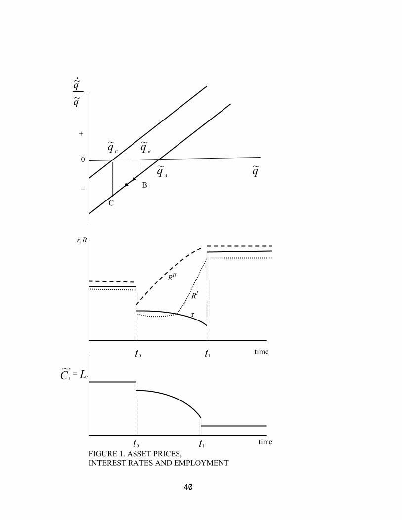
qq~~•

+ q C

~ q B~

0 q A

~ q~

_ B

C

r,R

RII

RI r t0

t time 1

LC t

s

t=~

t0

t1 time

FIGURE 1. ASSET PRICES, INTEREST RATES AND EMPLOYMENT

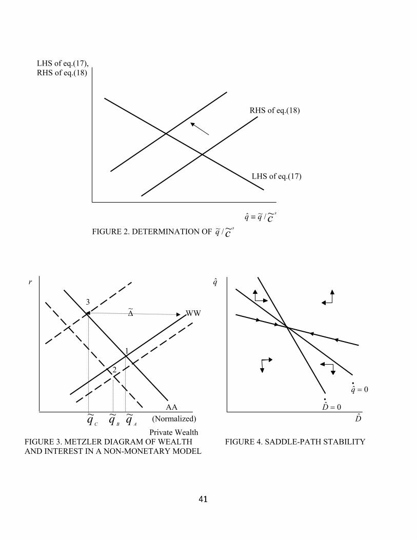
LHS of eq.(17), RHS of eq.(18) RHS of eq.(18) LHS of eq.(17) c sqq ~/~ˆ ≡

FIGURE 2. DETERMINATION OF q c s~/~ r q 3 ∆~ WW 1 2

q 0ˆ =•

AA 0ˆ =•

D q C

~ q B~ q A

~ (Normalized) D

Private Wealth FIGURE 3. METZLER DIAGRAM OF WEALTH FIGURE 4. SADDLE-PATH STABILITY AND INTEREST IN A NON-MONETARY MODEL

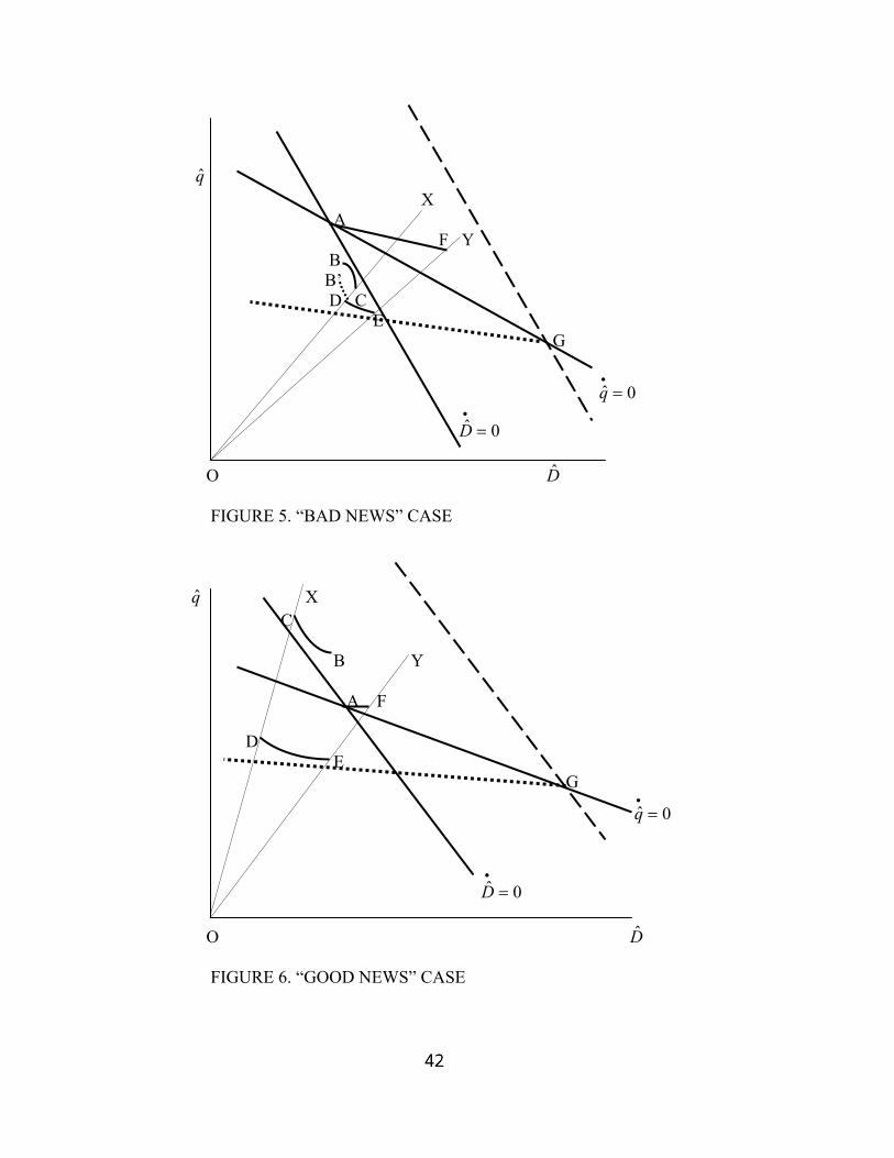
q

X A F Y B B’ D C E G

0ˆ =•

q

0ˆ =•

D O D FIGURE 5. “BAD NEWS” CASE X q C B Y A F D E G

0ˆ =•

q

0ˆ =•

D O D FIGURE 6. “GOOD NEWS” CASE