targeting debt and deficits in india: a structural ... · targeting debt and deficits in india: a...
TRANSCRIPT

1
Targeting Debt and Deficits in India: A Structural Macroeconometric Approach N R Bhanumurthy, Sukanya Bose and Parma Devi Adhikari
Working Paper No. 2015-148
May 2015
National Institute of Public Finance and Policy
New Delhi
http://www.nipfp.org.in
2
Targeting Debt and Deficits in India
A Structural Macroeconometric Approach a
N R Bhanumurthy, Sukanya Bose
and Parma Devi Adhikari *
Abstract
This study attempts to construct a consistent macroeconomic framework for India to review the macro-fiscal linkages over the 14
th Finance Commission period of
2015-19. The existing NIPFP model has been reworked to add a full-fledged real sector block comprising of agriculture, industry, services and infrastructure, with the overall economy comprising of real sector block, external block, monetary block, fiscal block and macroeconomic block. The estimated model was used for policy simulations that are relevant for the 14
th Finance Commission. The various scenarios
include (a) shock due to 7th Pay Commission award, (b) targeting deficit and debt and
(c) targeting higher growth. The results suggest that while Pay Commission award would result in slightly higher growth compared to the base case, this also results in higher inflation, fiscal-revenue deficits, current account deficit as well as higher government liability. Further simulation results suggest that expenditure switching policy, which is the core of expansionary fiscal consolidation mechanism, of increasing higher government capital expenditure and reducing the government transfers could result in higher growth with a manageable fiscal deficit of 5.3 per cent that also brings down the government (centre plus states) liability to around 60 per cent by 2019-20. JEL Classification: C32, E10, E17, E60, H60 Key Words: Fiscal consolidation, government debt, fiscal deficit, macroeconometric
modeling, India
a This is based on the larger report submitted to the 14th Finance Commission. The authors
would like to thank the Members and Research Staff of the 14th Finance Commission for their comments and suggestions on the draft report. The authors also like to thank Prof. V.N. Pandit for his insightful comments on the model framework. Abhishek Kumar and Swayamsiddha Panda have also contributed in the initial phase of this work. However, any omissions and errors in the paper are authors‟ alone. * The authors are with National Institute of Public Finance and Policy, New Delhi. E-mail for correspondence: [email protected]; [email protected]
3
Introduction
Global financial crisis and the expansionary fiscal policy measures, including the fiscal stimulus in the post-Crisis period, initiated in and around the Union Budget 2008-09 have led to higher fiscal deficits, much higher than those specified in the FRBM act, 2003. While those policies have helped in restraining further slowdown in the economy and helped in recovery in the two subsequent years, the nature of stimulus packages
1, which are largely irreversible in nature, appeared to have
resulted in deterioration of fiscal health. In order to revert to the fiscal consolidation path, therefore, the 13
th Finance Commission revised the fiscal road map. As per the
revised targets, Indian economy should achieve a fiscal deficit target of 5.4 per cent by 2014-15 while the debt-GDP ratio should be brought down to 68 per cent
2.
However, such targets were subject to some major assumptions on the exogenous factors such as external sector recovery and on the assumption of elimination of revenue deficit by 2014-15. As it turned out, the fragile recovery in the global growth and failure in reducing revenue deficit as per the revised fiscal consolidation path has made the feasibility of achieving the fiscal targets as suggested by the 13
th Finance
Commission almost impossible. In 2012-13, the economy experienced a sharp slowdown in growth along with
higher inflation, unsustainable current account deficits and higher fiscal deficits. It was an urgent necessity to review the fiscal deficit targets as prescribed by the 13
th
Finance Commission. Given the domestic and global environment, the Kelkar Committee (2012) revised and extended the fiscal deficit targets to 2016-17
3. Since
then, the Government has been trying to contain the fiscal deficits as per the revised targets. However, there appears to be a slippage on the sub-targets such as revenue deficit. For instance, as per the revised targets, the revenue deficit target for 2014-15 should have been 2 per cent compared to the Budget estimate of 2.9 per cent. At the same time there seems to be a slippage on the growth assumption as well
4. Such a
slippage on most of the indicators calls for revisiting of the fiscal deficit targets and suggesting conditions under which one can achieve the multiple objective of fiscal consolidation with stable growth.
With this background, this study attempts to review the macro-fiscal linkages
over the 14th Finance Commission period of 2015-19 with the help of consistent
macroeconomic framework for India. In the next section, some discussion on the revised NIPFP Macroeconomic Policy Simulation Model (MPSM) is provided. Here the approach is largely the Klein-Goldberger framework that follows structural macroeconometric method. In section-III databases and methodology used are discussed briefly. In section-IV, based on the assumptions on the exogenous variables, the model is simulated for both in-sample and out of sample. Diagnostic checking in terms of in-sample forecast performance and error behaviour is undertaken to establish the robustness of the model. As the purpose is to provide some policy inputs for the 14
th Finance Commission, two policy issues are discussed
in section-V. Simulation exercises are discussed in section-VI followed by the conclusion section.
1 See Mundle et al, 2011
2 Mundle, et al, 2010, showed that such fiscal targets are consistent with reasonably higher and
stable growth. 3 See the “Report of the Committee on Roadmap for Fiscal Consolidation: 2012”,
http://finmin.nic.in/reports/Kelkar_Committee_Report.pdf. These targets are only for Central Government. 4 Kelkar Committee (2012) assumes a nominal GDP growth of 15 per cent for 2014-15 against
the Union Budget assumption of 13.4 per cent.
4
II. Model Specification for the revised NIPFP Macroeconomic Policy Simulation Model
Macroeconomy is represented in terms of five blocks which are real sector
block, external sector block, fiscal block, monetary block and macroeconomic block.
Real Sector Block
The real sector of the economy has been disaggregated into four Sectors: Agriculture, Industry, Services and Infrastructure. The forces of demand and supply impact the price and output determination differently in the four sectors.
5
The four sectors are defined as per the NAS classification by economic activity.
(a) Agriculture includes agriculture, forestry and fishing (industry group 1).
(b) Industry includes mining & quarrying (industry group 2) and manufacturing (industry group 3).
(c) Services include trade, hotels and restaurants (industry group 6), finance, insurance and real estate (industry group 8) and community and social services (industry group 9).
(d) Infrastructure includes electricity, gas and water (industry group 4), construction (industry group 5) and transport, storage and communication (industry group 7).
Agriculture
All macro-models on the Indian economy have conceptualised the agriculture sector as a supply constrained sector with accumulation of capital constraining the level of value added. Krishnamurty, et al (2004) cast the relationship in terms of productivity of land. Yield per acre is a function of net fixed capital stock per acre and total agricultural credit per acre of land. The latter can be interpreted as the availability of working capital per unit of land.
To capture the effect of technology on capital productivity in agriculture, Sachdeva and Ghosh, 2009 have used area under HYV to total cropped area. Higher the area under HYV, higher the productivity of capital stock. Bhide and Parida (2009) postulate that higher value addition of agricultural products in agro-processing and allied sectors raises yield of agricultural production
6.
Most other models do not address agricultural productivity explicitly. Kar and
Pradhan (2009) determine real output as a function of capital stock and exogenously determined rainfall variable. Srivastava et al (2012) add to the specification of Kar and Pradhan by introducing the extent of irrigated area to total area as a determinant of output. Another complementary variable that releases supply bottlenecks in agriculture is infrastructure (power, road and other transport, storage). Murty and Soumya (2006) find that infrastructure output has a significant positive impact on agricultural output.
5 Also, there are differences in respect to fiscal variables. While agricultural incomes are
outside the direct tax net, the other sectors, particularly industrial sector, bears the burden of taxation. Public investment is crucial for all the productive sectors; infrastructure growth depends on fiscal policy support. 6 The variables, however, are not statistically significant in the estimated equation.
5
In models where the agriculture sector has been further disaggregated, relative prices across commodity groups have played a significant role (Bhide and Parida, 2009; Krishnamurty, et al, 2004). These models do not find a significantly positive price response of total agricultural output for the Indian economy.
We postulate the real agricultural output to be supply determined with
production dependent on net capital stock in agriculture and deviation of actual from normal rainfall. While the structural component of real agricultural output is a function of real capital stock at the end of the previous period, the cyclic component would depend upon the performance of rain, an exogenous variable. To bring in the price response of production, minimum support price (MSP) is added as an explanatory variable.
7
1) ZYFt
AGRI = f(ZNKt-1
AGRI, RAIN, MSP)
ZYFt
AGRI : Real agricultural GDP at factor cost
ZNKt-1AGRI
: Real net capital stock in agriculture (in previous period) RAIN: deviation of actual from normal rainfall (EXOGENOUS)
MSP: minimum support price (POLICY variable)
A set of identities link investments to net capital stock in agriculture. Addition to capital stock in agriculture between period t and t-1 takes place through net investment in period t (equation 2). Gross investment adjusted for depreciation is net investment (equation 3). Depreciation is assumed to be exogenous for the model.
2) ZNKt
AGRI = ZNIt
AGRI + ZNKt-1
AGRI
3) ZGI t
AGRI = ZNIt
AGRI + Depreciationt
AGRI
ZNIt
AGRI: Real net capital formation in agriculture
ZGItAGRI
: Real gross capital formation in agriculture Depreciationt
AGRI: Depreciation of capital stock in agriculture (EXOGENOUS)
Nominal gross investment in agriculture, derived from the real gross
investment in agriculture, is the sum of gross private and public investment in agriculture.
4) GI tAGRI
≡ Pt AGRI
* ZGIt AGRI
≡ GIPUt AGRI
+ GIPVt AGRI
GIt
AGRI: Nominal gross investment in agriculture
GIPVtAGRI
: Nominal gross private investment in agriculture GIPUt
AGRI: Nominal gross public investment in agriculture
PtAGRI :
Price deflator of agriculture sector The sectoral investment functions for all the sectors of the Indian economy, including agriculture, display an accelerator relationship with output. Besides, there is strong complementarity with public investment in agriculture (Mani, et al, 2011). Real investment in agriculture is presumed to be independent of interest rate changes, because of the preferential treatment of the sector in credit policies. Models like
7 Net irrigated area and the area under HYV (as a proportion to total cropped area) have been
stagnant over the last few years, and therefore were not included in the model specification. Institutional credit to meet the working capital needs of the agriculture sector affects real agricultural output. However, when introduced along with capital stock in agriculture, the variable suffers from multicollinearity problem.
6
Krishnamurty et al (2004) and Bhide and Parida (2009) have included credit growth in the private investment function, since most actors in this sector are up against supply rationing in the credit market. Higher availability of institutional credit for the farm sector would lead to higher capital formation in agriculture. We postulate private investment to depend upon the nominal output in the agriculture sector and having complementarity with ) public investment in agriculture.
5) GIPV tAGRI
= f(YFtAGRI
, GIPU tAGRI
)
YFtAGRI
: GDP at factor cost in the agriculture sector.
Public investment in agriculture is a function of capital expenditure by government (combined, Centre and States) on agriculture. All government capital expenditure does not flow into investment and all public investment does not come from the government budget alone, since it is supplemented by investment of internal surpluses of public sector undertakings. However, the two are closely correlated.
6) GIPU t
AGRI = f(ECAP t
AGRI)
7) ECAP t
AGRI ≡ a1. ECAPt
where ECAP t
AGRI is capital expenditure by government in agriculture
(nominal); ECAPt is total capital expenditure by government (nominal); a1: policy determined ratio of proportion of capital expenditure going to agriculture.
8
Agricultural prices are determined by a combination of supply and demand factors. Kar and Pradhan (2009) estimate a simple function with real output in agriculture and private disposable income for determining agricultural prices. Besides, government‟s activity in agricultural markets has an important bearing on agricultural prices. The government sets the MSP which has a positive impact on prices. The government has an important role in determining the net availability of foodgrains through its stock-holding operations and public distribution system. Krishnamurty (1984) had introduced per capita net availability of food grains (net production plus change in government stocks plus net imports) to represent the supply conditions in the foodgrain market.
9 Alongside real factors, monetary factors
have been used in a few models. In Krishnamurty et al (2004), M3/GDP is a common determinant of price level in all the sectors of the economy.
We postulate agricultural prices to be determined by a combination of supply
and demand factors and MSP. The equation is cast in terms of change in agriculture prices. Change in agricultural prices is a function of change in MSP, change in private consumption demand in the economy and the cyclical component of real output of agricultural sector.
8) d(P t
AGRI) = f( d(CPR t), d(MSP), Cyc_ZYFt
AGRI)
P t
AGRI: Price deflator of the agricultural sector.
CPR t: Private consumption
8 While we have attempted to relate the budgetary capital expenditure with public investment,
the relation is subject to certain practical limitations. Indian Public Finance Statistics reports the capital expenditure of the government in terms of functional heads, whereas the National Accounts Statistics reports public investments under economic heads. At times, this gives rise to incongruity among the capital expenditure and public investment numbers. 9 Bhide and Parida (2009) have used net availability as a determinant of price of rice.
7
Cyc_ZYFtAGRI
: Cyclic component of ZYFtAGRI
Industry
Industrial output in any year can be seen as a product of the productive capacity of the industrial sector and the utilization of the installed capacity, while industrial capacity utilization is mainly determined by demand side variables (Kar and Pradhan, 2009).
10
Different studies have used different sets of variables to represent the
demand side: real compensation to employees (Bhide and Parida, 2009), agricultural output and autonomous expenditure where the latter is measured as government expenditure and exports of goods and services (Kar and Pradhan, 2009), real public consumption, investment plus exports (Krishnamurty et al, 2004).
In Krishnamurty et al, 2004 real output in manufacturing is modeled as a
product of capital stock and productivity of capital stock.11
The latter is a function of both demand side and supply side variables. The supply side variables include the real infrastructural output per unit of real capital stock in the manufacturing sector to explain the productivity of manufacturing. Two other variables on the intensity of input use in manufacturing are the non-food agricultural output and real import of crude and other mineral oils, chemicals etc (as a proportion of real capital stock in the manufacturing sector).
Bhide and Parida (2009) introduce the effect of FDI-induced technological
changes as a determinant in the output equation. FDI in mining, quarrying and manufacturing reflects the impact of growing integration of the economy with the international markets through adoption of modern technology and practices on productivity. This variable is found to be significant.
We hypothesize a demand side specification for industrial output, given the
predominantly demand constrained nature of the sector. Industrial output in real terms is postulated as a function of overall investment demand in the economy and export demand for goods in the economy where both the demand side variables are expressed in real terms. Since a large part of the industrial output is produced to meet the investment requirements of industry and other sectors, a slowdown in investment demand affects the industrial sector the maximum.
9) ZYFt
INDUS = f (Xt
G/Pt
INDUS , GIt / Pt
INDUS )
ZYFt
INDUS: real output of the industrial sector at factor cost
GIt: gross total investment Xt
G: exports of goods (nominal)
PtINDUS
: price deflator of industrial goods
A set of identities similar to identities (2) to (4) in the agriculture sector link net capital stock to gross investment in the industrial sector.
10
In the reduced form equation on real industrial output, capacity utilization is substituted by its determinants. 11
Sachdeva and Ghosh (2009) macro-consistency model use a similar approach across the three sectors (agriculture, industry and services).
8
Gross investment in industry is the sum of private and public investment in industry
12.
10) GIt
INDUS = GIPUt
INDUS + GIPVt
INDUS
GIt
INDUS : gross investment in industry
GIPUtINDUS
: gross public investment in industry GIPVt
INDUS : gross private investment in industry
Private investment in industry is determined by (a) monetary and credit
conditions; (b) expected output growth (accelerator) (c) complementarity with public investment. The last of these relationships, between public investment and private investment, is an oft debated one though there is strong evidence of the importance of public sector investment to revive and sustain industrial and economy-wide growth.
13 Several studies have thus tried to empirically explore crowding in and
crowding out through the industrial investment function. In Krishnamurty et al (2004) higher gross investment (total) is supposed to affect private investment in manufacturing positively, while public investment (total) along with private investment in agriculture, by competing for investible resources, tends to affect it adversely. The authors obtain statistically significant evidence of crowding out as per the above definition. Kar and Pradhan (2009) find that the impact of public investment in industry is positive on private investment in the industrial sector, but the impact of higher government consumption expenditure is negative. The problem with Kar and Pradhan‟s specification is the presence of a close relationship between the two independent variables – public consumption expenditure and public investment. As we discuss later in the Fiscal Block, higher public consumption may itself cause the capital expenditure and public investment to decline given fiscal deficit targets.
We postulate private investment function in industry on the lines of Mundle et al (2011). It is an accelerator type private investment function, where private investment is assumed to depend on the cost of capital as well as the crowding in effect of public investment, and the expected rate of capacity utilization. This economy-wide investment function in Mundle et al (2011) has been taken to be valid for the industrial sector.
11) GIPV t
INDUS / YMPt = f[INTRATEt, (GIPU t
INDUS /YMP t), ZYF t-1
INDUS/ C(ZYF t-1
INDUS)]
INTRATEt: lending rate by commercial banks ZYF t-1
INDUS: Real output of the industrial sector in the previous period.
C(ZYF t-1INDUS
): Capacity output of the industrial sector in the previous period.
The rate of private investment in industry is determined by interest rate, public investment rate in industry and previous years‟ capacity utilization rate. C(ZYF t
INDUS) or the capacity output of the industrial sector is derived by multiplying
the actual capital stock with the inverse of the trend component of capital output ratio in the industrial sector.
12) C(ZYF tINDUS
) ≡ (1/ KOR_TREND tINDUS
) * ZNKt
INDUS
12
See appendix B figure no.1 for share of public investment in total sectoral investment (public and private). 13
See Chakraborty (1988) “Some current issues in economic policy” in Development Planning.
9
ZNKtINDUS
: Real Net Capital Stock in Industry.
KOR_TREND tINDUS
is the trend component of the capital output ratio in the industrial sector after removing the cyclical component. This variable can be viewed as representative of the industrial technology. KOR_TREND t
INDUS shows a secularly
rising trend since the mid-1990s (See appendix B, figure 2 on sectoral capital-output ratio, HP-Trend).
Gross public investment in industry is linked to budgetary capital expenditure in industry through a link equation. And capital expenditure on industry is a fraction, a2, of the total capital expenditure.
13) GIPU tINDUS
= f(ECAP tINDUS
)
14) ECAP tINDUS
≡ a2. ECAPt
Where ECAP tINDUS
is capital expenditure by government in industry (nominal); ECAPt is total capital expenditure by government (nominal); a2 is policy determined proportion of capital expenditure going to industry.
In contrast to agricultural prices which are determined by demand and supply conditions after controlling for the impact of administered pricing, industrial prices exhibit cost-plus pricing. Econometric models have thus used cost factors in the industrial price specification. We specify industrial price (measured as industrial price deflator) as a function of its own past value, agricultural prices, domestic oil prices and money supply (net capital flows plus bank credit). Agricultural prices and domestic oil prices represent the cost of certain essential inputs for the industrial sector, whereas the lagged value of industrial prices is to capture the price stickiness. Higher net capital flows and bank credit, used as a proxy for money supply, exerts an upward pressure on industrial prices.
15) PtINDUS
= f(Pt-1INDUS
, PtAGRI
, PtOIL
, Net Capital Flowst) Pt
INDUS : price of industrial goods
PtAGRI
: price of agricultural goods Pt
OIL: administered price of oil (POLICY variable)
Net Capital Flowst: Net international capital flows to India
16) PtOIL
= f(OILPRUSDt, OILPRRATIOt) OILPRUSDt: International price of Indian basket of oil imports (EXOGENOUS)
OILPRRATIOt is the ratio of domestic oil price index divided by the
international oil price index in Rupee terms. This is also called the pass-through ratio. Given the international oil prices, higher the pass-through ratio, higher is the domestic oil price. Services
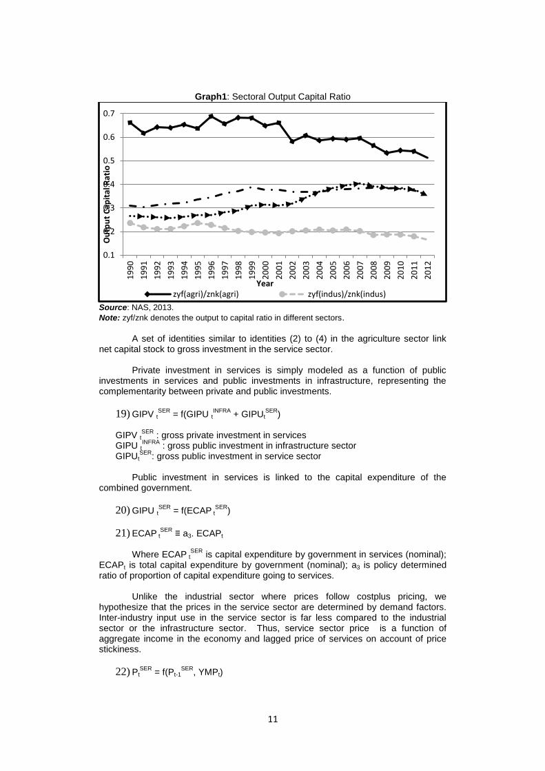
Service sector has witnessed substantial gains in productivity unlike other sectors of the Indian economy in the years since 1991 (see Graph 1 for capital productivity in services). Rakshit (2007) notes that while there has been a decline in growth of capital stock in services, output growth in the sector continued to be high, due to increases in total factor productivity. In general, volume of investment required is moderate and technological adaption is faster and easier in the service sector.
10
Demand side factors have played a crucial role in raising total factor productivity in service sector in India argues Nell (2013).Thus, most macroeconometric models have found growth of real output in the service sector being explained by demand side variables. Alternate specifications to capture the importance of demand (either directly in the output function or as a determinant of productivity of capital stock) include: real output of non-service sector (Krishnamurty et al, 2004, Kar and Pradhan, 2009), real compensation to employees (Bhide and Parida, 2009); private disposable income and government consumption (Srivastava et al, 2012); agricultural and industrial output and all exports, including invisibles (Sachdeva and Ghosh, 2009).
Besides the demand side factors, increase in total factor productivity in service sector can be explained by: (a) nature of production involving low intensity of capital and financial requirements, release of infrastructure bottlenecks and (b) FDI encouraged through favourable fiscal policies and presence of high skilled labour. Bhide and Parida (2004) find significant impact on service sector growth of supply of infrastructure and FDI in the sector.
We model the real output of the service sector as a product of productivity of capital stock and capital stock in service sector. Service productivity in turn is explained by domestic consumption needs (private and public) as well as external demand for services.
17) ZYFtSER
= ZNKtSER
* (Z YFtSER
/ ZNKtSER
)
18) ZYFtSER
/ ZNKtSER
= ( NXtSER
/PtSER
, CPUt +CPRt/Pt
SER)
ZYFt
SER : real output of the service sector at factor cost
ZNKtSER
: real net capital stock of the service sector NXt
SER: net exports of services
PtSER
: price of services CPRt: Private consumption demand CPUt: Public consumption demand
Public consumption of services not only adds to demand for services from the
demand side but can be considered as an essential input from the supply side to raise productivity of services. Public expenditure on education, health and other social services raises overall productivity of services in the economy in the medium and long run.
11
Graph1: Sectoral Output Capital Ratio
Source: NAS, 2013.
Note: zyf/znk denotes the output to capital ratio in different sectors.
A set of identities similar to identities (2) to (4) in the agriculture sector link net capital stock to gross investment in the service sector.
Private investment in services is simply modeled as a function of public
investments in services and public investments in infrastructure, representing the complementarity between private and public investments.
19) GIPV tSER
= f(GIPU tINFRA
+ GIPUtSER
) GIPV t
SER : gross private investment in services
GIPU tINFRA
: gross public investment in infrastructure sector GIPUt
SER: gross public investment in service sector
Public investment in services is linked to the capital expenditure of the
combined government.
20) GIPU tSER
= f(ECAP tSER
)
21) ECAP tSER
≡ a3. ECAPt
Where ECAP tSER
is capital expenditure by government in services (nominal); ECAPt is total capital expenditure by government (nominal); a3 is policy determined ratio of proportion of capital expenditure going to services.
Unlike the industrial sector where prices follow costplus pricing, we
hypothesize that the prices in the service sector are determined by demand factors. Inter-industry input use in the service sector is far less compared to the industrial sector or the infrastructure sector. Thus, service sector price is a function of aggregate income in the economy and lagged price of services on account of price stickiness.
22) PtSER
= f(Pt-1SER
, YMPt)
0.1
0.2
0.3
0.4
0.5
0.6
0.7
19
90
19
91
19
92
19
93
19
94
19
95
19
96
19
97
19
98
19
99
20
00
20
01
20
02
20
03
20
04
20
05
20
06
20
07
20
08
20
09
20
10
20
11
20
12
Ou
tpu
t C
apit
al R
atio
Year zyf(agri)/znk(agri) zyf(indus)/znk(indus)
12
PtSER
: Price deflator of the service sector YMPt: nominal GDP at market price
Infrastructure
Infrastructure sector consists of the subsectors (a) electricity, gas and water; (b) construction; and (c) transport, storage and communication. Infrastructure figures as a separate sector in very few macro models. Infrastructure investment by the government (exogenously given) enters as a determinant in private investment functions of other sectors (RBI, 2002). Krishnamurty et al (2004) treat economic activity in infrastructure sector as supply driven. Further, they find that public infrastructure investments crowds in private investment significantly.
We hypothesize infrastructure output as a function of real net capital stock in infrastructure sector.
23) ZYFtINFRA
= f (ZNKt-1INFRA
) ZYFt
INFRA : real output of the infrastructure sector at factor cost
ZNKt-1INFRA
: real net capital stock of the infrastructure sector at the end of the previous period.
A set of identities similar to identities (2) to (4) in the agriculture sector link net capital stock to gross investment in the infrastructure sector.
Private investment in infrastructure is dependent on the level of economic
activity (accelerator relationship), interest rate (cost of borrowing) and public investment in infrastructure (complementarity of investments).
24) GIPVtINFRA
= f(GIPU tINFRA
, INTRATEt, YMPt ) GIPV t
INFRA : gross private investment in infrastructure sector
GIPU tINFRA
: gross public investment in infrastructure sector
Public investment in infrastructure is linked to the capital expenditure of the combined government.
25) GIPU tINFRA
= f(ECAP tINFRA
)
26) ECAP tINFRA
≡ a4. ECAPt
Where ECAP tINFRA
is capital expenditure by government on infrastructure (nominal); ECAPt is total capital expenditure by government (nominal); a4: policy determined ratio of proportion of capital expenditure going to infrastructure sector. Infrastructure prices (Pt
INFRA) is a function of its own past values and industrial
commodity price (PtINDUS
), the latter capturing the inter-sectoral linkages.
27) PtINFRA
= f(Pt-1INFRA
,Pt INDUS
)
13
EXTERNAL SECTOR BLOCK
With growing integration of the domestic economy with the rest of the world, there are a number of channels through which external shocks transmit to the domestic economy. External sector is a major source of demand for sectoral output, as seen above. Higher growth in rest of the world causes export demand for goods and services to rise and vice-versa. On the other hand, higher domestic growth translates to higher import demand both for intermediate use and final consumption.
Trade flows along with flows on the income account comprise the current
account balance of the balance of payments for the economy. Current account balance (as a proportion of overall economic activity), an indicator of external balance, is a key policy target for developing economies. Remittance income and net investment income are the two flows on the income account of the current account of the balance of payments. The remittance income increases with higher growth of advanced economies and Middle East economies, while the net investment income is related to net capital flows. The specifications of the components of current account of BOPs are discussed below.
14
Export of goods is a function of World GDP, exchange rate and import
weighted average tariff rate. The tariff rate captures the competitiveness of Indian exports (see Mundle et al, 2010).
28) XtG = f(WORLDGDPt, DUTYt, ERt)
Xt
G: export of goods
WORLDGDPt: world GDP (EXOGENOUS) ERt: exchange rate (EXOGENOUS)
15
DUTYt: import weighted average tariff rate (EXOGENOUS) Import of goods is a function of nominal output, international oil prices and exchange rate. Higher the international price of oil, higher is the import bill.
29) MtG = f(YMPt, ERt, OILPRUSDt )
Mt
G: import of goodsOILPRUSDt: oil price in US Dollars (EXOGENOUS)
Net exports of services are dependent on the level of GDP of the US, since it
is the major destination country for India‟s exports of services. Merchandise exports exert a positive influence on service exports due to network effects wherein a country with high penetration in goods market can use its networks to export services.
30) NXtSER
= f(XtG, USGDPt)
NXt
SER: net export of services
USGDPt: US GDP (EXOGENOUS)
14
The external sector block has been discussed in further detail and greater level of disaggregation in Bhanumurthy et al (2014). Krishnamurthy and Pandit (1997) present a moderately disaggregative model of India‟s trade flows covering the period 1971-91. 15
In Bhanumurthy et al (2014) exchange rate is endogenous, determined by the macroeconomic balance approach.
14
Remittances rise with the rise in domestic interest rate and the income in the source countries measured as the sum of GDP of Middle East and Advanced Economies.
31) REMITt = f(MEGDPt + ADVGDPt, INTRATEt)
REMITt: remittances MEGDPt: Middle East GDP (EXOGENOUS) ADVGDPt : GDP of the advanced countries (EXOGENOUS) INTRATEt : lending rates of banks
The last component of the current account of BOP is the net investment income. Net investment income has been deteriorating in the recent years. With persistently high current account deficit, great capital inflows have been required to balance the external accounts, which in turn give rise to greater outflows in investment income. Net investment income is negatively related to net capital flows and exchange rate.
32) NETINVESTINCOMEt = f(NETCAPITALFLOWSt, ERt)
NETINVESTINCOMEt : Net investment income NETCAPITALFLOWSt : Net capital flows (Inflows minus Outflows in the capital account)
Most macro-models assume capital flows to be autonomous beyond the
control of national authorities. Another noteworthy fact about capital flows is their procyclical nature. We model net capital flows as a function of nominal income to reflect the procyclical nature of capital flows. Further, credit rating is a forward looking variable that captures the future prospects of the economy. Credit rating of a country is based on its institutional and governance effectiveness, economic structure and growth prospects, external liquidity and international investment position, fiscal performance and monetary flexibility. By influencing the perceived investment climate, credit rating affects net capital flows positively. Interest rate plays a role in determining international debt flows, but is found to have little influence on the aggregate net capital flows.
33) NETCAPITALFLOWSt = f(YMPt , CREDITRATINGt)
CREDITRATINGt : Credit rating (EXOGENOUS) Current account balance (CAB) is represented by the following identity:
34) CABt = XtG
- MtG
+ NXtSER
+REMITt+NETINVESTINCOMEt FISCAL BLOCK
Fiscal block has important policy levers consisting of expenditure and revenue measures to steer the economy both from the demand side as well as supply side. This is vital in the context of growth-inflation and fiscal imbalances, and particularly relevant to the 14
th Finance Commission,
Revenue receipts of the combined government comprise of direct tax revenue, indirect tax revenue and non-tax revenue. The change in direct tax revenue of government is given by:
15
35) d(DTAX)t 1t d(YMP) t /YMPt-1 ] DTAXt-1
DTAXt : Direct tax b1t : Direct tax buoyancy (POLICY variable) YMPt : Nominal income It is assumed that the government can influence the buoyancy through adjustments in tax rates and the administrative tax effort. Similarly, the change in indirect tax revenue of government is given by:
36) d(INDTAX)t t d(YMP) t /YMPt-1 INDTAXt-1 INDTAXt : Indirect tax b2t : Indirect tax buoyancy (POLICY variable) Non-Tax revenue is assumed to be a function of nominal income.
37) NONTAXREVt = f(YMPt) NONTAXREVt: Non Tax revenue in year t. Revenue Receipts (REVRECt ) is represented by the following identity
38) REVRECt= DTAXt + INDTAXt + NONTAXREVt
Revenue Expenditure in year t is given by the following identity:
39) REVEXPt OTHERECURRt+ TRANSFERSt+ INTERESTPAYt REVEXPt : Revenue Expenditure in year t OTHERECURRt: Other Revenue Expenditure in year t. TRANSFERSt : Transfer payments by government inclusive of subsidies (EXOGENOUS). INTERESTPAYt : Interest Payment on Government Liabilities.
OTHERECURR is the budgetary counterpart to government consumption
expenditure. It includes the salaries and wages component of the government budget and is sticky upwards; it is assumed to depend on its own past values.
40) OTHERECURRt = f(OTHERECURRt-1)
Interest payments can be represented by the following identity comprising of liabilities at the end of the last period and rate of interest on government securities in the last period.
41) INTERESTPAYt≡ LIABt-1 * ROIGSECt-1 LIABt-1: Stock of government liabilities outstanding at the end of the previous period ROIGSECt-1: Interest rate on government securities in the previous period
16
Transfer payments by government inclusive of subsidies (TRANSFERS) is assumed to be a discretionary policy variable for the model.
16
Revenue Deficit (REVDEFICITt) is given by
42) REVDEFICITt REVEXPt – REVRECt
Capital expenditure of the government is a crucial policy variable with important links with the real sector as seen in the real sector block. Bose and Bhanumurthy (2013) obtain a capital expenditure multiplier of 2.4 for the Indian economy. However, this important component of government expenditure is often squeezed to make space for other kinds of expenditure. Empirically it has been found that higher the revenue deficit smaller is the capital expenditure, given fiscal deficit target (see Appendix B, Fig 4). Thus we postulate capital expenditure to be a declining function of revenue deficit.
43) ECAPt = f(REVDEFICITt)
ECAPt : Capital Expenditure in year t
Capital expenditure by the government is divided into sectoral capital expenditure. Apart from the sectoral shares, about 15-25 per cent of total capital expenditure is defense related. A substantial part of this expenditure is spent on imports and has no linkage with productive sectors in the economy.
17
44) ECAPt ≡ ECAP tAGRI
+ ECAP tINDUS
+ ECAP tSER
+ ECAP tINFRA
+ ECAPtDEF
The fiscal deficit in year t (FDt) is given by
45) FDt REVDEFICITt +ECAPt -NDCRt d(D t) + d(FR t) NDCRt : Non-Debt Capital Receipts (EXOGENOUS) d(D t) : Change in government debt d(FR t) : Change in fiscal reserves. (EXOGENOUS)
Financing of fiscal deficit occurs through change in debt, d(D)t, and change in
fiscal reserves, d(FR)t. Besides debt financing part of the fiscal deficit has been met through drawdown of cash balances in recent times.
18
Market borrowing and other borrowings of the government add to the stock of
debt. 19
46) d(Dt) MBt + OBt MBt : market borrowing of the government
16
Transfers include all subsidies of the government. In Bhanumurthy et al (2012) oil subsidy was endogenised and modeled as a function of oil price pass-through and international oil price. The linkages of oil sector to the macroeconomy could be integrated due to the flexible nature of the model. In the present version of the model this link is absent and subsidies are integrated with transfers, which in turn are assumed to be discretionary. 17
Refer to appendix B, Figure no.3. 18
With discontinuation of the 91-day tap treasury bills, the concept of conventional budget deficit has lost its relevance since April 1, 1997. 19
Refer to appendix B, Figure 7 on liability and debt-GDP ratio.
17
OBt : other borrowing of the government such as the proportions of small savings and provident funds used to finance fiscal deficit (EXOGENOUS)
20
Market borrowing is assumed to be a function of fiscal deficit
47) MBt= f(FDt) Note that government debt to finance fiscal deficit is a subset of total
government liabilities, the difference ranging from 7 to 15 per cent of GDP across years. In other words, debt is a part of total liabilities used for financing FD.
48) LIABt Dt + OLt
LIABt: Stock of government liabilities outstanding in period t OLt : Other liabilities includes liabilities on account of NSSF, State Provident Funds, Other Accounts and reserve funds not accounted for in Dt (EXOGENOUS) 21
Primary deficit (PDt) is given by
49) PDt FDt -INTERESTPAYt
MONETARY BLOCK
Repo rate is a policy parameter for the Central bank. With inflation control being the principal objective of the RBI, repo rate (REPO) is supposed to respond to the gap between actual and desired inflation rate. 5 per cent is the present desired benchmark inflation rate.
50) REPOt = f(PWPIt)-.05, REPOt-1),
PWPIt :Overall wholesale price index REPOt : Repo rate
The central bank responds to inflation and at the same time there is interest rate persistence. REPO rate transmits the monetary policy signals to the economy via other interest rates, namely the lending rate of commercial banks (INTRATE) and interest rate on government securities (ROIGSEC). Interest rate on government securities is assumed directly to be a function of policy rate (Repo). 51) ROIGSECt = f(REPOt)
Lending rate of commercial banks (INTRATE) is positively related to REPO and the government‟s market borrowing. The government being a large borrower, higher market borrowing by the government can cause upward pressure on lending rate. Crowding out presumes a buoyant demand for credit from the private sector.
52) INTRATEt = f(REPOt , MBt)
Disbursal of non-food bank credit by the commercial banks is assumed to be demand determined. Higher the investment demand in the economy, higher the demand for non-food bank credit which is met through credit expansion by banks.
20
See IPFS, 2012-13 Table 4.7 21
Government Debt Status Paper, MoF 2013.
18
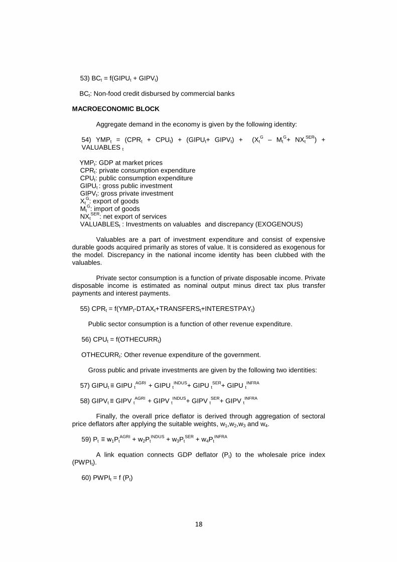
53) BCt = f(GIPUt + GIPVt) BCt: Non-food credit disbursed by commercial banks MACROECONOMIC BLOCK
Aggregate demand in the economy is given by the following identity:
54) YMPt = (CPRt + CPUt) + (GIPUt+ GIPVt) + (XtG – Mt
G+ NXt
SER) +
VALUABLES t YMPt: GDP at market prices CPRt: private consumption expenditure CPUt: public consumption expenditure GIPUt : gross public investment GIPVt: gross private investment Xt
G: export of goods
MtG: import of goods
NXtSER
: net export of services VALUABLESt : Investments on valuables and discrepancy (EXOGENOUS) Valuables are a part of investment expenditure and consist of expensive durable goods acquired primarily as stores of value. It is considered as exogenous for the model. Discrepancy in the national income identity has been clubbed with the valuables. Private sector consumption is a function of private disposable income. Private disposable income is estimated as nominal output minus direct tax plus transfer payments and interest payments.
55) CPRt = f(YMPt-DTAXt+TRANSFERSt+INTERESTPAYt)
Public sector consumption is a function of other revenue expenditure.
56) CPUt = f(OTHECURRt) OTHECURRt: Other revenue expenditure of the government. Gross public and private investments are given by the following two identities: 57) GIPUt ≡ GIPU t
AGRI + GIPU t
INDUS+ GIPU t
SER+ GIPU t
INFRA
58) GIPVt ≡ GIPV t
AGRI + GIPV t
INDUS+ GIPV t
SER+ GIPV t
INFRA
Finally, the overall price deflator is derived through aggregation of sectoral
price deflators after applying the suitable weights, w1,w2,w3 and w4.
59) Pt ≡ w1PtAGRI
+ w2PtINDUS
+ w3PtSER
+ w4PtINFRA
A link equation connects GDP deflator (Pt) to the wholesale price index
(PWPIt).
60) PWPIt = f (Pt)
19
III. Database and Methodology for Estimation
The model has been estimated using annual data for the period 1991-92 to 2012-13. In some cases, as the final NAS data for 2012-13 such as sectoral investments were not available at the time of estimations, the estimation is limited to 2011-12. The data definitions and the sources are presented in appendix-A. In terms of estimation procedures, simple OLS method has been used.
As the 2008 crisis has created instability in most of the parameters, to adjust
its impact a dummy variable has been introduced. Structural dummies are introduced in order to capture the structural breaks in the dependent variables. Structural breaks were estimated using Bai-Perron test. To correct for autocorrelation, autoregressive (AR1) terms are introduced. However, in the estimated equations, there are some outliers in the errors, which could be for various unexplainable reasons and may not be explained by the theoretical variables. In order to minimise such errors and derive the robust parameters that can explain the underlying macroeconomic behaviour, outlier dummies are introduced. Such adjustments in outliers are largely similar to the Error Correction Mechanism models that help in deriving underlying long term behaviour after correcting for errors. The estimated equations are solved together by using Gauss-Seidel algorithm for the latest period, i.e., for 2009-2012. Depending on the extent of errors in the in-sample period, the model can be used for out of sample simulations.
Appendix C presents the regression results for the estimated equations of the
model.
IV. Variables of Interest
All the estimated equations together with identities are solved for the recent period to assess the forecast performance of the whole model. The key policy variables in solving this model include revenue and capital expenditure, tax buoyancy, minimum support prices, the policy interest rates, and government borrowing. The important exogenous variables include the growth of output in OECD countries as a group as well as in the USA and the Middle East; world oil prices; exchange rate, depreciation rates, and the rainfall index. A scenario is designed by setting the value of both the policy variables as well as the exogenous variables. The outcome variables of interest in each scenario include the growth rate, the inflation rate and the total liability-GDP ratio as well as some other key macroeconomic ratios, i.e., the investment rate; the trade deficit and current account deficit relative to GDP; the tax-GDP ratio, the revenue deficit-GDP ratio and the fiscal deficit-GDP ratio.
Empirical Validation
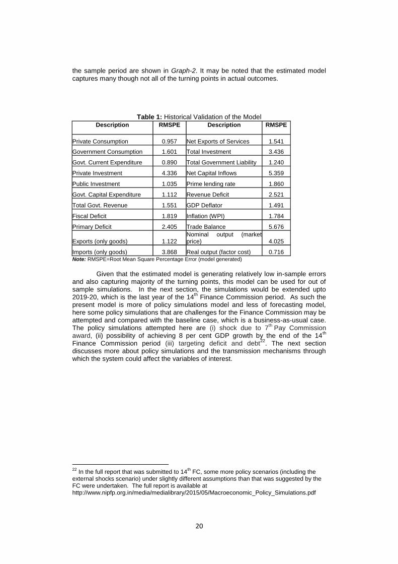
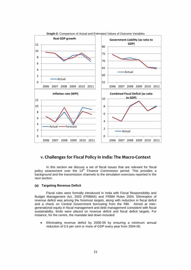
The model has been estimated using annual data for the period 1991-92 to 2012-13, taking care of time series properties. The standard diagnostic tests have also been applied. The model has been solved for the sample period 2009-10 to 2012-13 and validated for this period. The root mean square percentage errors for all the key variables are shown in table 1. Except for net capital inflows and trade balance, which model shows slightly higher than acceptable RMSPE of 5 per cent, the rest of the variables RMSPE is within 5 percent. This suggests that the estimated model is robust and performs well against actual outcomes for the sample period. To see if the estimated model tracks the turning points, which is another key feature of a robust model, the plots of estimated outcome variables against their actual values in
20
the sample period are shown in Graph-2. It may be noted that the estimated model captures many though not all of the turning points in actual outcomes.
Table 1: Historical Validation of the Model Description RMSPE Description RMSPE
Private Consumption 0.957 Net Exports of Services 1.541
Government Consumption 1.601 Total Investment 3.436
Govt. Current Expenditure 0.890 Total Government Liability 1.240
Private Investment 4.336 Net Capital Inflows 5.359
Public Investment 1.035 Prime lending rate 1.860
Govt. Capital Expenditure 1.112 Revenue Deficit 2.521
Total Govt. Revenue 1.551 GDP Deflator 1.491
Fiscal Deficit 1.819 Inflation (WPI) 1.784
Primary Deficit 2.405 Trade Balance 5.676
Exports (only goods) 1.122 Nominal output (market price) 4.025
Imports (only goods) 3.868 Real output (factor cost) 0.716 Note: RMSPE=Root Mean Square Percentage Error (model generated)
Given that the estimated model is generating relatively low in-sample errors
and also capturing majority of the turning points, this model can be used for out of sample simulations. In the next section, the simulations would be extended upto 2019-20, which is the last year of the 14
th Finance Commission period. As such the
present model is more of policy simulations model and less of forecasting model, here some policy simulations that are challenges for the Finance Commission may be attempted and compared with the baseline case, which is a business-as-usual case. The policy simulations attempted here are (i) shock due to 7
th Pay Commission
award, (ii) possibility of achieving 8 per cent GDP growth by the end of the 14th
Finance Commission period (iii) targeting deficit and debt22
. The next section discusses more about policy simulations and the transmission mechanisms through which the system could affect the variables of interest.
22
In the full report that was submitted to 14th FC, some more policy scenarios (including the
external shocks scenario) under slightly different assumptions than that was suggested by the FC were undertaken. The full report is available at http://www.nipfp.org.in/media/medialibrary/2015/05/Macroeconomic_Policy_Simulations.pdf
21
Graph-2: Comparison of Actual and Estimated Values of Outcome Variables
V. Challenges for Fiscal Policy in India: The Macro-Context
In this section we discuss a set of fiscal issues that are relevant for fiscal policy assessment over the 14
th Finance Commission period. This provides a
background and the transmission channels to the simulation exercises reported in the next section.
(a) Targeting Revenue Deficit
Fiscal rules were formally introduced in India with Fiscal Responsibility and
Budget Management Act, 2003 (FRBMA) and FRBM Rules 2004. Elimination of revenue deficit was among the foremost targets, along with reduction in fiscal deficit and a check on Central Government borrowing from the RBI. Aimed at inter-generational equity in fiscal management and debt management consistent with fiscal sustainability, limits were placed on revenue deficit and fiscal deficit targets. For instance, for the centre, the mandate laid down included:
Eliminating revenue deficit by 2008-09 by ensuring a minimum annual reduction of 0.5 per cent or more of GDP every year from 2004-05.
0
2
4
6
8
10
12
2006 2007 2008 2009 2010 2011
Actual
Real GDP growth
0
2
4
6
8
10
12
2006 2007 2008 2009 2010 2011
Inflation rate (WPI)
Actual Forecast
55
60
65
70
75
80
2006 2007 2008 2009 2010 2011
Government Liability (as ratio to GDP)
Actual
0
2
4
6
8
10
2006 2007 2008 2009 2010 2011
Combined Fiscal Deficit (as ratio to GDP)
Actual
22
Reducing fiscal deficit by at least 0.3 per cent of GDP annually from 2004-05, so that fiscal deficit is reduced to no more than 3 per cent of GDP at the end of 2008-09.
Similarly for the states, 12
th Finance Commission recommended that each
state enact Fiscal Responsibility Legislation (FRL) which should, at the minimum, provide for elimination of revenue deficit by 2008-09 and reduction of fiscal deficit to 3 per cent of GSDP or its equivalent defined as ratio of interest payment to revenue receipts to be brought down to 15 per cent
23. Following this pre-condition stipulated
by 12th Finance Commission, all states put in place FRL as per State Finances.
Debt-relief was provided to the states working towards fiscal consolidation. The quantum of write-off was linked to the absolute amount by which the revenue deficit was reduced in each successive year during the award period.
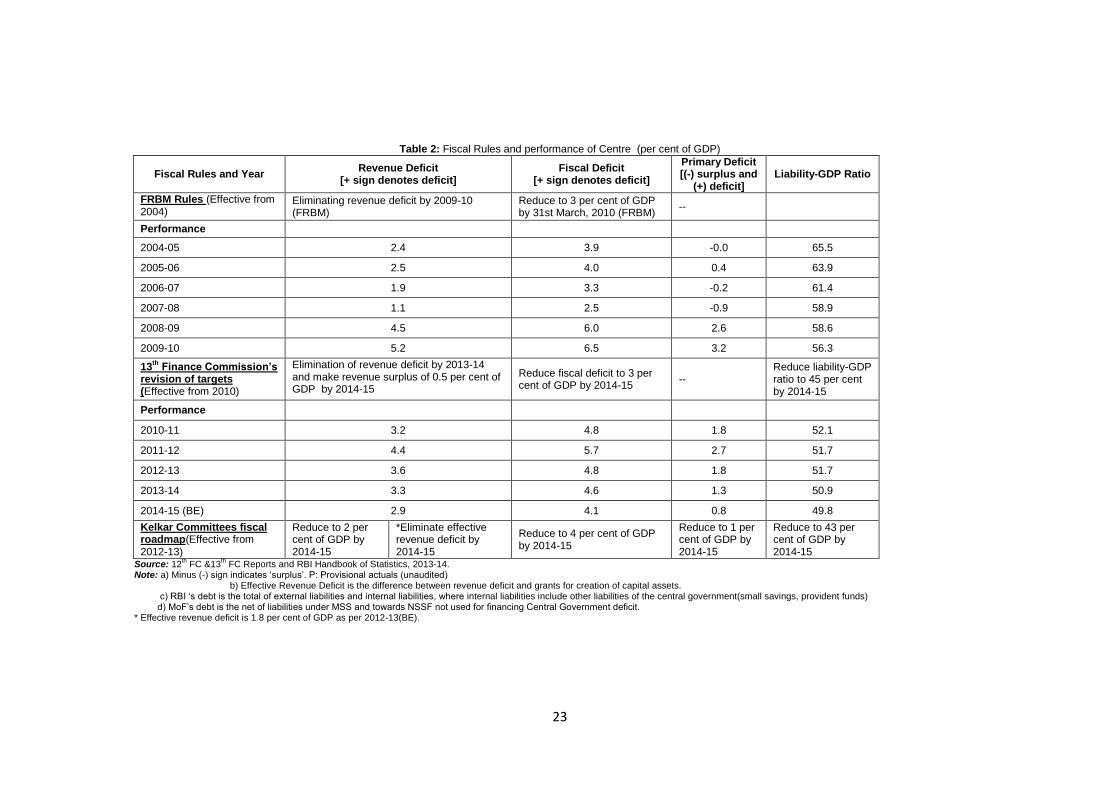
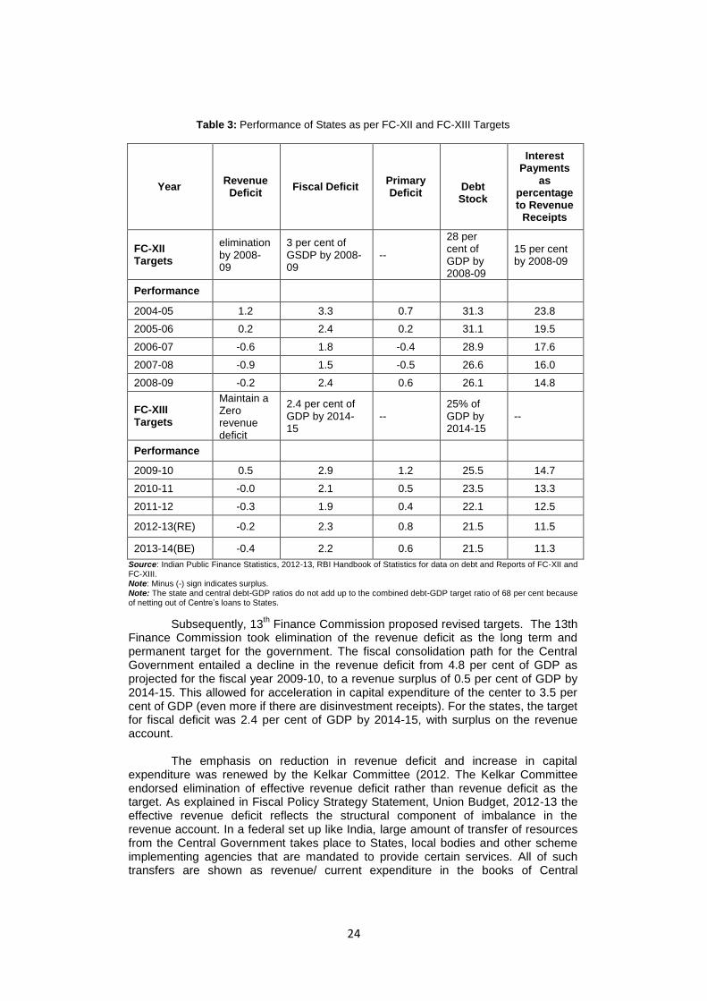
Consequent to the buoyant economic growth and revenues in the years since
2003-04, fiscal rules brought about substantial improvements in fiscal balances. The performance of the center and states vis-à-vis the fiscal rules are summarized in Table 2 and Table 3 below. The global financial crisis, slowdown in domestic growth and need for countercyclical fiscal stimulus caused a temporary pause in fiscal consolidation.
23
pp.87, 12th FC Report.
23
Table 2: Fiscal Rules and performance of Centre (per cent of GDP)
Fiscal Rules and Year Revenue Deficit
[+ sign denotes deficit] Fiscal Deficit
[+ sign denotes deficit]
Primary Deficit [(-) surplus and
(+) deficit] Liability-GDP Ratio
FRBM Rules (Effective from 2004)
Eliminating revenue deficit by 2009-10 (FRBM)
Reduce to 3 per cent of GDP by 31st March, 2010 (FRBM)
--
Performance
2004-05 2.4 3.9 -0.0 65.5
2005-06 2.5 4.0 0.4 63.9
2006-07 1.9 3.3 -0.2 61.4
2007-08 1.1 2.5 -0.9 58.9
2008-09 4.5 6.0 2.6 58.6
2009-10 5.2 6.5 3.2 56.3
13th
Finance Commission’s revision of targets (Effective from 2010)
Elimination of revenue deficit by 2013-14 and make revenue surplus of 0.5 per cent of GDP by 2014-15
Reduce fiscal deficit to 3 per cent of GDP by 2014-15
-- Reduce liability-GDP ratio to 45 per cent by 2014-15
Performance
2010-11 3.2 4.8 1.8 52.1
2011-12 4.4 5.7 2.7 51.7
2012-13 3.6 4.8 1.8 51.7
2013-14 3.3 4.6 1.3 50.9
2014-15 (BE) 2.9 4.1 0.8 49.8
Kelkar Committees fiscal roadmap(Effective from 2012-13)
Reduce to 2 per cent of GDP by 2014-15
*Eliminate effective revenue deficit by 2014-15
Reduce to 4 per cent of GDP by 2014-15
Reduce to 1 per cent of GDP by 2014-15
Reduce to 43 per cent of GDP by 2014-15
Source: 12th FC &13
th FC Reports and RBI Handbook of Statistics, 2013-14.
Note: a) Minus (-) sign indicates „surplus‟. P: Provisional actuals (unaudited) b) Effective Revenue Deficit is the difference between revenue deficit and grants for creation of capital assets. c) RBI „s debt is the total of external liabilities and internal liabilities, where internal liabilities include other liabilities of the central government(small savings, provident funds) d) MoF‟s debt is the net of liabilities under MSS and towards NSSF not used for financing Central Government deficit. * Effective revenue deficit is 1.8 per cent of GDP as per 2012-13(BE).
24
Table 3: Performance of States as per FC-XII and FC-XIII Targets
Year Revenue
Deficit Fiscal Deficit
Primary Deficit
Debt Stock
Interest Payments
as percentage to Revenue
Receipts
FC-XII Targets
elimination by 2008-09
3 per cent of GSDP by 2008-09
--
28 per cent of GDP by 2008-09
15 per cent by 2008-09
Performance
2004-05 1.2 3.3 0.7 31.3 23.8
2005-06 0.2 2.4 0.2 31.1 19.5
2006-07 -0.6 1.8 -0.4 28.9 17.6
2007-08 -0.9 1.5 -0.5 26.6 16.0
2008-09 -0.2 2.4 0.6 26.1 14.8
FC-XIII Targets
Maintain a Zero revenue deficit
2.4 per cent of GDP by 2014-15
-- 25% of GDP by 2014-15
--
Performance
2009-10 0.5 2.9 1.2 25.5 14.7
2010-11 -0.0 2.1 0.5 23.5 13.3
2011-12 -0.3 1.9 0.4 22.1 12.5
2012-13(RE) -0.2 2.3 0.8 21.5 11.5
2013-14(BE) -0.4 2.2 0.6 21.5 11.3
Source: Indian Public Finance Statistics, 2012-13, RBI Handbook of Statistics for data on debt and Reports of FC-XII and FC-XIII. Note: Minus (-) sign indicates surplus. Note: The state and central debt-GDP ratios do not add up to the combined debt-GDP target ratio of 68 per cent because of netting out of Centre‟s loans to States.
Subsequently, 13th Finance Commission proposed revised targets. The 13th
Finance Commission took elimination of the revenue deficit as the long term and permanent target for the government. The fiscal consolidation path for the Central Government entailed a decline in the revenue deficit from 4.8 per cent of GDP as projected for the fiscal year 2009-10, to a revenue surplus of 0.5 per cent of GDP by 2014-15. This allowed for acceleration in capital expenditure of the center to 3.5 per cent of GDP (even more if there are disinvestment receipts). For the states, the target for fiscal deficit was 2.4 per cent of GDP by 2014-15, with surplus on the revenue account.
The emphasis on reduction in revenue deficit and increase in capital expenditure was renewed by the Kelkar Committee (2012. The Kelkar Committee endorsed elimination of effective revenue deficit rather than revenue deficit as the target. As explained in Fiscal Policy Strategy Statement, Union Budget, 2012-13 the effective revenue deficit reflects the structural component of imbalance in the revenue account. In a federal set up like India, large amount of transfer of resources from the Central Government takes place to States, local bodies and other scheme implementing agencies that are mandated to provide certain services. All of such transfers are shown as revenue/ current expenditure in the books of Central
25
Government. However, significant proportion of such transfers is specifically meant for creation of capital assets which are public goods in nature. To protect such expenditures, it was recommended that revenue deficit after netting out the above-kind of expenditures, may be targeted. Thus, Kelkar Committee, September 2012, on the fiscal roadmap of the Central Government recommended that fiscal deficit be reduced to 4 per cent of GDP, effective revenue deficit to be eliminated and revenue deficit to be reduced to 2 percent of GDP by 2014-15.Overall there was a shift in emphasis towards capital expenditure within the fiscal consolidation framework. This had empirical support in research studies. Bose and Bhanumurthy (2013) based on the previous NIPFP macroeconomic model had estimated the value of the capital expenditure multiplier to be greater than 2. Thus any increase in capital expenditure would cause the nominal incomes to more than double. Revenue expenditure multiplier on the other hand was close to 1.
While the emphasis on higher capital expenditure is well-placed there are
genuine concerns about compression of revenue expenditure. For instance, an important question is how to treat expenditures on education and health. It has been argued that since development on account of health and education gets embodied in the beneficiaries once health standards improve or educational standards are stepped up, the expenditure incurred on these is more akin to investment and hence, it would be fair to treat it as capital expenditure. Moreover, in the absence of nurses, doctors and teachers, the capital expenditure incurred on hospital buildings or school buildings is of little use.
24 Thus, Rakshit (2010) notes that, “given the overarching
requirement of non-negative revenue balance, clubbing HRD expenditures with current ones not only leaves little scope for enlarging investment in human capital, but the stipulated FRBM targets might in all probability be met through a slowdown in HRD spending”.
(b) Debt Stabilization Issues
It is generally argued that a rise in the debt-GDP Ratio is a concern as large
interest payments on public debt jeopardises the plan to raise development expenditure and also stands in the way of provision of essential public goods. Secondly, a higher market borrowing to finance the growing debt may lead to a higher rate of interest and thus crowd out private investment. Further, debt might be considered problematic for fiscal solvency. Two key factors affecting solvency are the response of primary balance (i.e. the budget balance net of interest payments on the debt) to increases in debts and the possibility of adverse shocks. It is assumed that when debt gets very large, it may be difficult to generate a primary balance that is sufficient to ensure sustainability, and that shocks can push countries beyond their debt limit (Chowdhury and Islam, 2010).
There are three important concepts regarding debt-GDP ratio: stability,
sustainability and optimality. Stability implies a constant debt ratio with time. Sustainability means the returns from additional borrowing should be greater than or equal to cost of additional borrowing. Chronic excess of government expenditure over revenue receipts financed through borrowing from the public is said to be sustainable if in the long run the ratio of public debt to national income stabilizes or does not rise without limit. Optimality refers to debt level, beyond which there is a negative relationship with growth.
24
The 13th
FC recognized this issue, but didn‟t act upon it (See13th FC Report, pp.129).
26
Optimal Debt and Growth: What does the Empirical Literature Say?
Some of the recent empirical literature has explored the relationship between debt-GDP and growth. An oft quoted paper by Reinhert and Rogoff (2010) seems to suggest that beyond 90 per cent there may be a negative relation between debt and growth. Reinhart and Rogoff, 2010 (RR henceforth) have categorized the countries in four public debt brackets (0-30, 30-60, 60-90, and above 90 per cent of GDP) across time and have noted the growth rate corresponding to the different debt levels. They calculate a composite growth rate for each debt category by assigning weights to countries. Composite growth rates are calculated for advanced economies and emerging market economies separately. The authors‟ claim that the median growth declines substantially beyond 90 per cent debt-GDP level and the average growth becomes negative beyond 90 per cent threshold for advanced economies. The same approach with emerging economies indicates lower median growth rate beyond 90 per cent, but the average growth rate after 90 per cent debt level is not found to be negative. The findings of RR were countered by, Herndon, Ash, and Pollin (2013) who identified coding errors and selective weighing in RR methodology. In fact, after carrying out some formal tests, Herndon, Ash, and Pollin (2013) report that differences in average GDP growth in the categories 30-60 percent, 60-90 percent, and 90-120 percent cannot be statistically distinguished.
The negative relationship between growth and debt levels become more
suspect as it is driven by presence of a few strong outlier countries (with very high debt and low growth combinations) and the endogenity has not been controlled for. The latter is particularly important for developing countries. There is a strong positive empirically robust relationship between a few of the economic variables which government expenditure can largely influence (like initial years of schooling) and GDP growth (IMF, 2010). The growth-inhibiting effects of a given percentage increase in debt-to-GDP ratio can be easily overwhelmed by a given percentage increase in growth-promoting variables achieved through public spending. It is therefore argued that it is important to look at the composition of debt, instead of just focusing on the aggregate value of debt. (Chowdhury and Islam, 2010).
Domar (1944) put forward the sustainability condition for the debt-financing of
government expenditure. According to Domar if the government finances part of its expenditure (amounting to a given fraction of full employment output) through borrowing, in a growing economy public debt and government‟s interest outgo as proportions of GDP will be stable in the long run provided the growth rate exceeds the interest rate. The implication is that when the Domar condition is satisfied, maintenance of full employment through debt-financing of fiscal deficits does not erode the fiscal deficit or produce a debt-trap.
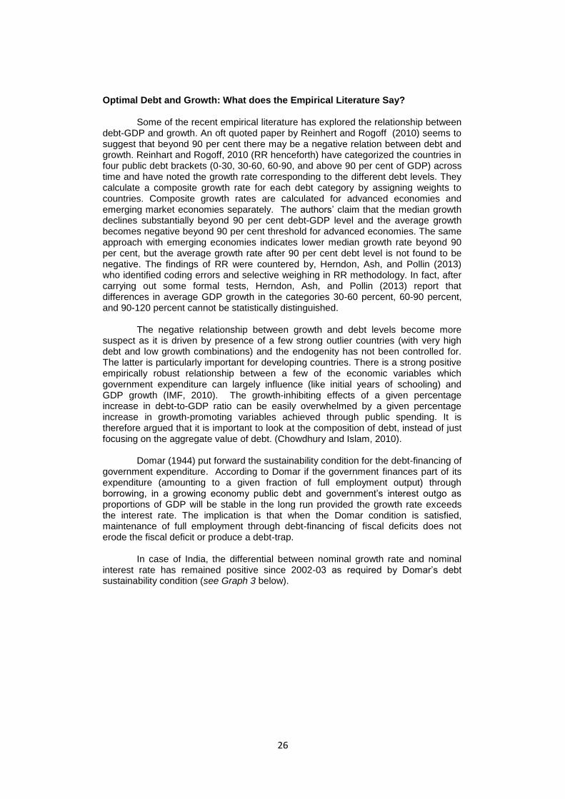
In case of India, the differential between nominal growth rate and nominal
interest rate has remained positive since 2002-03 as required by Domar‟s debt sustainability condition (see Graph 3 below).
27
Graph 3: Differential between Nominal Growth Rate and Nominal Interest Rate for the Indian
Economy
Source: Data for GDP from NAS, Statement 1 and rate of interest on Government securities is the simple average of weighted average of interest rate on state government and central government securieties.The data is from, RBI, HBS,2013.
Rangarajan and Srivastava (2005) have looked at debt-stabilization wherein debt-GDP ratio is unvarying across time. This requires a stricter set of condition on deficits than required by Domar. The necessary and sufficient conditions for debt-stability are discussed below:
Necessary Condition: The GDP growth rate is higher than interest rate (if the
growth rate is equal to interest rate the debt ratio will rise linearly and if the growth rate is lesser than interest rate the debt ratio would raise exponentially).
Sufficient Condition: Primary deficit is equal or less than the debt stabilizing
level of primary deficit. The debt-stabilizing primary deficit is derived as under from the debt-GDP equation, Equation (1).
= + [(1+ )/(1+ )] ------(1)
Where, =Debt to GDP Ratio in period t.
= Primary Deficit to GDP Ratio
= rate of interest
= Growth rate of GDP
For debt-GDP stability we require that = . If debt-GDP is stable then we have the debt-stabilizing primary deficit as follows from (1):
= - [(1+ )/(1+ )] = [1- (1+ )/(1+ )] = - )/(1+ ) ---------------(2)
As long as in any given year is equal to or less than for that year, the
debt-GDP ratio will not rise in that year compared to its level in previous year. Note
that depends on the previous year’s debt-GDP ratio, growth rate and interest rate.
-0.05
0.05
0.15
0.25
19
91
-92
19
92
-93
19
93
-94
19
94
-95
19
95
-96
19
96
-97
19
97
-98
19
98
-99
19
99
-00
20
00
-01
20
01
-02
20
02
-03
20
03
-04
20
04
-05
20
05
-06
20
06
-07
20
07
-08
20
08
-09
20
09
-10
20
10
-11
20
11
-12
20
12
-13
Year r g g-r
28
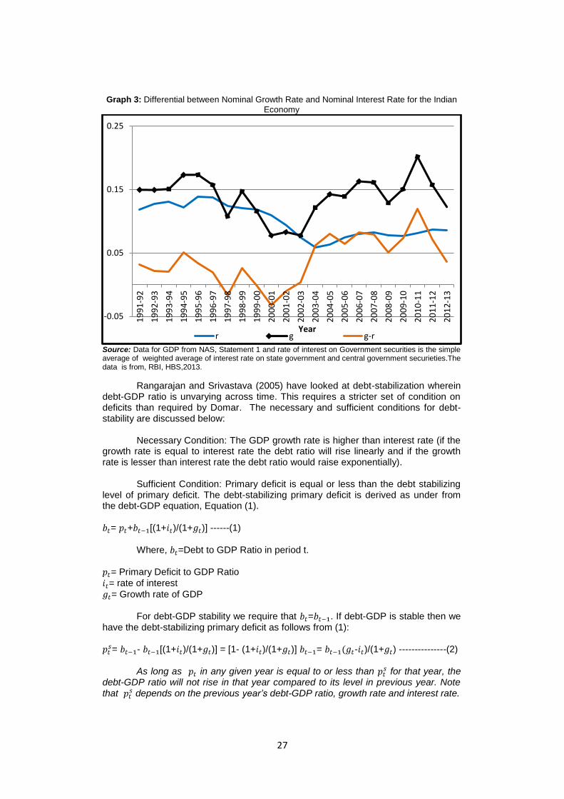
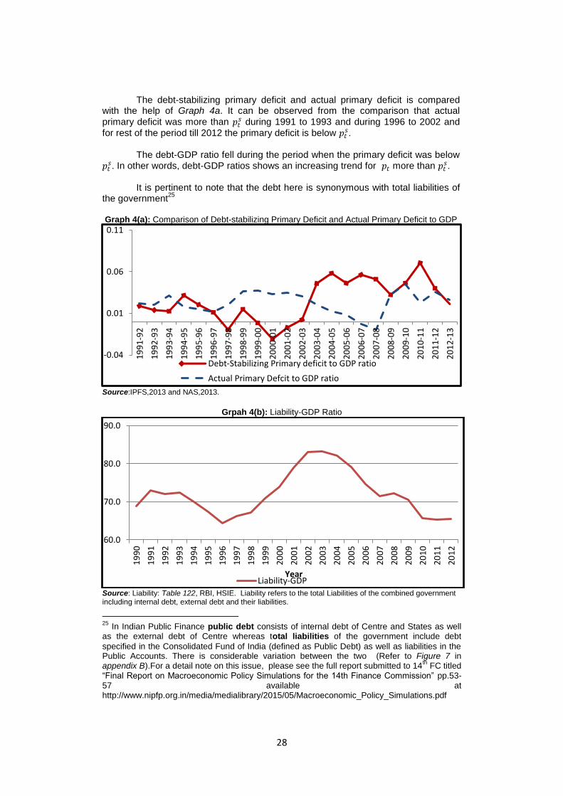
The debt-stabilizing primary deficit and actual primary deficit is compared with the help of Graph 4a. It can be observed from the comparison that actual
primary deficit was more than during 1991 to 1993 and during 1996 to 2002 and
for rest of the period till 2012 the primary deficit is below . The debt-GDP ratio fell during the period when the primary deficit was below
. In other words, debt-GDP ratios shows an increasing trend for more than .
It is pertinent to note that the debt here is synonymous with total liabilities of the government
25
Graph 4(a): Comparison of Debt-stabilizing Primary Deficit and Actual Primary Deficit to GDP
Source:IPFS,2013 and NAS,2013.
Grpah 4(b): Liability-GDP Ratio
Source: Liability: Table 122, RBI, HSIE. Liability refers to the total Liabilities of the combined government including internal debt, external debt and their liabilities.
25
In Indian Public Finance public debt consists of internal debt of Centre and States as well as the external debt of Centre whereas total liabilities of the government include debt
specified in the Consolidated Fund of India (defined as Public Debt) as well as liabilities in the Public Accounts. There is considerable variation between the two (Refer to Figure 7 in appendix B).For a detail note on this issue, please see the full report submitted to 14
th FC titled
“Final Report on Macroeconomic Policy Simulations for the 14th Finance Commission” pp.53-57 available at http://www.nipfp.org.in/media/medialibrary/2015/05/Macroeconomic_Policy_Simulations.pdf
-0.04
0.01
0.06
0.11
19
91
-92
19
92
-93
19
93
-94
19
94
-95
19
95
-96
19
96
-97
19
97
-98
19
98
-99
19
99
-00
20
00
-01
20
01
-02
20
02
-03
20
03
-04
20
04
-05
20
05
-06
20
06
-07
20
07
-08
20
08
-09
20
09
-10
20
10
-11
20
11
-12
20
12
-13
Debt-Stabilizing Primary deficit to GDP ratio
Actual Primary Defcit to GDP ratio
60.0
70.0
80.0
90.0
19
90
19
91
19
92
19
93
19
94
19
95
19
96
19
97
19
98
19
99
20
00
20
01
20
02
20
03
20
04
20
05
20
06
20
07
20
08
20
09
20
10
20
11
20
12
Year Liability-GDP
29
The debt-GDP stability condition can also be developed using the concept of
fiscal deficit.Let us assume fiscal deficit in period t is defined as:
= - ----(3)
where, are Outstanding debt of government in period t and t-1 respectively.
Dividing (3) by GDP in perod t ( ) we get,
= is the growth rate of GDP in period t.
= – ------(4)
Where, , symbolizes ratios of fiscal deficit and debt to GDP.
If = = , then the debt-stabilizing fiscal deficit to GDP ratio is
= ----(5)
Also, the stable debt-GDP ratio in terms of stable fiscal deficit to GDP is
= ---------(6)
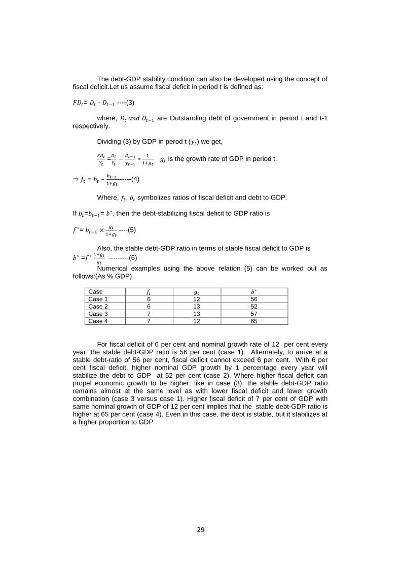
Numerical examples using the above relation (5) can be worked out as follows:(As % GDP)
Case
Case 1 6 12 56
Case 2 6 13 52
Case 3 7 13 57
Case 4 7 12 65
For fiscal deficit of 6 per cent and nominal growth rate of 12 per cent every year, the stable debt-GDP ratio is 56 per cent (case 1). Alternately, to arrive at a stable debt-ratio of 56 per cent, fiscal deficit cannot exceed 6 per cent. With 6 per cent fiscal deficit, higher nominal GDP growth by 1 percentage every year will stabilize the debt to GDP at 52 per cent (case 2). Where higher fiscal deficit can propel economic growth to be higher, like in case (3), the stable debt-GDP ratio remains almost at the same level as with lower fiscal deficit and lower growth combination (case 3 versus case 1). Higher fiscal deficit of 7 per cent of GDP with same nominal growth of GDP of 12 per cent implies that the stable debt-GDP ratio is higher at 65 per cent (case 4). Even in this case, the debt is stable, but it stabilizes at a higher proportion to GDP
30
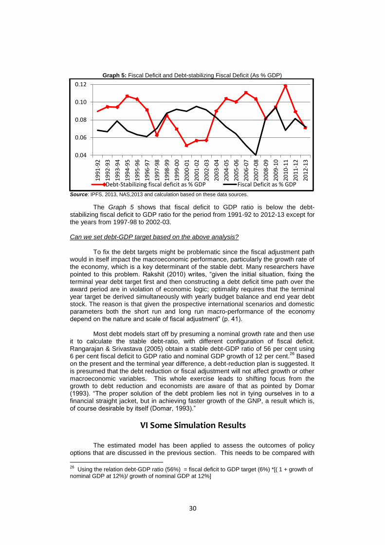
Graph 5: Fiscal Deficit and Debt-stabilizing Fiscal Deficit (As % GDP)
Source: IPFS, 2013, NAS,2013 and calculation based on these data sources.
The Graph 5 shows that fiscal deficit to GDP ratio is below the debt-stabilizing fiscal deficit to GDP ratio for the period from 1991-92 to 2012-13 except for the years from 1997-98 to 2002-03.
Can we set debt-GDP target based on the above analysis?
To fix the debt targets might be problematic since the fiscal adjustment path would in itself impact the macroeconomic performance, particularly the growth rate of the economy, which is a key determinant of the stable debt. Many researchers have pointed to this problem. Rakshit (2010) writes, “given the initial situation, fixing the terminal year debt target first and then constructing a debt deficit time path over the award period are in violation of economic logic; optimality requires that the terminal year target be derived simultaneously with yearly budget balance and end year debt stock. The reason is that given the prospective international scenarios and domestic parameters both the short run and long run macro-performance of the economy depend on the nature and scale of fiscal adjustment” (p. 41).
Most debt models start off by presuming a nominal growth rate and then use
it to calculate the stable debt-ratio, with different configuration of fiscal deficit. Rangarajan & Srivastava (2005) obtain a stable debt-GDP ratio of 56 per cent using 6 per cent fiscal deficit to GDP ratio and nominal GDP growth of 12 per cent.
26 Based
on the present and the terminal year difference, a debt-reduction plan is suggested. It is presumed that the debt reduction or fiscal adjustment will not affect growth or other macroeconomic variables. This whole exercise leads to shifting focus from the growth to debt reduction and economists are aware of that as pointed by Domar (1993). “The proper solution of the debt problem lies not in tying ourselves in to a financial straight jacket, but in achieving faster growth of the GNP, a result which is, of course desirable by itself (Domar, 1993).”
VI Some Simulation Results
The estimated model has been applied to assess the outcomes of policy options that are discussed in the previous section. This needs to be compared with
26
Using the relation debt-GDP ratio (56%) = fiscal deficit to GDP target (6%) *[( 1 + growth of nominal GDP at 12%)/ growth of nominal GDP at 12%]
0.04
0.06
0.08
0.10
0.12
19
91
-92
19
92
-93
19
93
-94
19
94
-95
19
95
-96
19
96
-97
19
97
-98
19
98
-99
19
99
-00
20
00
-01
20
01
-02
20
02
-03
20
03
-04
20
04
-05
20
05
-06
20
06
-07
20
07
-08
20
08
-09
20
09
-10
20
10
-11
20
11
-12
20
12
-13
Debt-Stabilizing fiscal deficit as % GDP Fiscal Deficit as % GDP
31
the base case, which is the business-as-usual case. To derive the base case upto 2019-20, one has to extend the exogenous variables with certain assumptions. The assumptions on the exogenous variables are as follows:
1. On the external front, the growth rates of advanced countries, Middle East
and the World GDP is assumed to grow as per the projections provided by the IMF. The import weighted average tariffs (duty) are assumed to remain at the same level as at present, i.e., 10 per cent. The exchange rate, which is the crucial variable in the external account, is assumed to be at 60. International oil price of USD 802 per MT has been assumed for 2013-14 based on RBI data. From 2014-15, international oil price is assumed at USD 720 per MT which is equivalent to $100 per barrel (approx.).
2. Depreciation rates at the sector level assumed to be at the 2012-13 level, which is the latest information that is available. The capital-output ratio in the industrial sector assumed to increase as per the trend growth. Given that India has a stable government at the moment, the credit rating is assumed to be positive.
3. Minimum support prices are assumed to increase at an average growth of 5 per cent. In the case of rainfall, except for 2014-15, which is assumed to be 10 per cent below normal, it is assumed to be normal for the rest of the period.
4. Oil price pass-through ratio is expected to increase from the current level of 60 per cent to 65 percent.
5. Share of valuables, which includes discrepancy, is assumed to be at 3.3 per cent of GDP, which is the last five years average. As valuables is mostly estimated as residual and highly volatile, modeling such behaviour is difficult.
6. Direct and indirect tax buoyancies are 1.48 and 1.42 respectively, for 2013-14 as per 2013-14(BE) and direct tax buoyancy and indirect tax buoyancy are assumed to be 1.1 from 2014-15 onwards. Non-debt capital receipts, which are largely disinvestment proceeds, are assumed to be at a modest level of 0.2 per cent of GDP based on recent trends. In the case of sectoral capital expenditures, the shares in the recent year are expected to continue for the rest of the forecast period. Similarly, for valuables (including discrepancy) and transfers within the revenue expenditures, its share in the GDP at market prices in 2012-13 is assumed for the forecast period. Since there is no actual data available for 2013-14 and 2014-15, as per the
14 Finance Commission recommendations, the Budgeted numbers (on both deficits as well as revenue buoyancies) are used for these years.
27 In our view, going by the
recent trends where the actual deficit numbers are higher than Budgeted (except in one year when there was windfall gains due to spectrum auction), such assumption itself could underestimate the fiscal numbers in the forecast period. Even the buoyancy assumption of over 1.4 for 2013-14 is also on the higher side as such higher buoyancies are experienced only in the pre-Crisis period.
27
For the year 2013-14, revised estimates for total tax revenue (center plus state combined) is not available yet. However, comparable figures for the center indicate large differences between BE and RE figures for 2013-14. Center‟s direct tax buoyancy estimates are 1.13 (RE) versus 1.58 (BE). And center‟s indirect tax buoyancy estimates are 0.77 (RE) versus 1,55 (BE) in 2013-14.
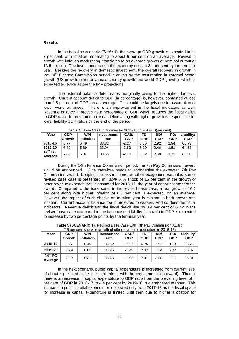
32
Results
In the baseline scenario (Table 4), the average GDP growth is expected to be 7 per cent, with inflation moderating to about 6 per cent on an average. Revival in growth with inflation moderating, translates to an average growth of nominal output at 13.5 per cent. The investment rate in the economy rises to 34 per cent by the terminal year. Besides the recovery in domestic investment, the overall recovery in growth in the 14
th Finance Commission period is driven by the assumption in external sector
growth (US growth, other advanced country growth and world GDP growth), which is expected to revive as per the IMF projections.
The external balance deteriorates marginally owing to the higher domestic
growth. Current account deficit to GDP (in percentage) is, however, contained at less than 2.5 per cent of GDP, on an average. This could be largely due to assumption of lower world oil prices. There is an improvement in the fiscal indicators as well. Revenue balance improves as a percentage of GDP which reduces the fiscal deficit to GDP ratio. Improvement in fiscal deficit along with higher growth is responsible for lower liability-GDP ratios by the end of the period.
Table 4: Base Case Outcomes for 2015-16 to 2019-20(per cent)
Year GDP Growth
WPI Inflation
Investment rate
CAB/ GDP
FD/ GDP
RD/ GDP
PD/ GDP
Liability/ GDP
2015-16 6.77 6.49 33.32 -2.27 6.76 2.92 1.94 66.73
2019-20 6.89 5.89 33.94 -2.53 6.29 2.46 1.51 64.53
14th
FC Average
7.00 6.04 33.65 -2.44 6.52 2.69 1.71 65.68
During the 14th Finance Commission period, the 7th Pay Commission award
would be announced. One therefore needs to endogenise the expected 7th Pay Commission award. Keeping the assumptions on other exogenous variables same, revised base case is presented in Table 5. A shock of 15 per cent in the growth of other revenue expenditures is assumed for 2016-17, the year of announcement of the award. Compared to the base case, in the revised base case, a real growth of 0.6 per cent along with higher inflation of 0.3 per cent is expected, on an average. However, the impact of such shocks on terminal year is minimal in both growth and inflation. Current account balance too is projected to worsen. And so does the fiscal indicators. Revenue deficit and the fiscal deficit rise by 0.9 per cent of GDP in the revised base case compared to the base case. Liability as a ratio to GDP is expected to increase by two percentage points by the terminal year.
Table 5 (SCENARIO 1): Revised Base Case with 7th Pay Commission Award
(15 per cent shock in growth of other revenue expenditure in 2016-17)
Year GDP Growth
WPI Inflation
Investment rate
CAB/ GDP
FD/ GDP
RD/ GDP
PD/ GDP
Liability/ GDP
2015-16 6.77 6.49 33.32 -2.27 6.76 2.92 1.94 66.73
2019-20 6.99 6.01 33.96 -3.45 7.37 3.54 2.44 66.37
14th
FC Average
7.59 6.31 33.65 -2.92 7.41 3.58 2.55 66.31
In the next scenario, public capital expenditure is increased from current level
of about 4 per cent to 4.4 per cent (along with the pay commission award). That is, there is an increase in capital expenditure to GDP ratio from the prevailing level of 4 per cent of GDP in 2016-17 to 4.4 per cent by 2019-20 in a staggered manner. This increase in public capital expenditure is allowed only from 2017-18 as the fiscal space for increase in capital expenditure is limited until then due to higher allocation for
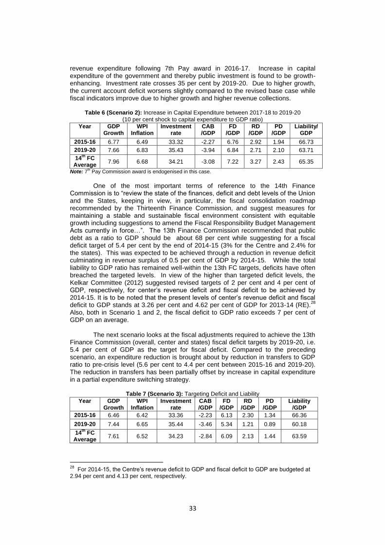
33
revenue expenditure following 7th Pay award in 2016-17. Increase in capital expenditure of the government and thereby public investment is found to be growth-enhancing. Investment rate crosses 35 per cent by 2019-20. Due to higher growth, the current account deficit worsens slightly compared to the revised base case while fiscal indicators improve due to higher growth and higher revenue collections.
Table 6 (Scenario 2): Increase in Capital Expenditure between 2017-18 to 2019-20
(10 per cent shock to capital expenditure to GDP ratio)
Year GDP Growth
WPI Inflation
Investment rate
CAB /GDP
FD /GDP
RD /GDP
PD /GDP
Liability/ GDP
2015-16 6.77 6.49 33.32 -2.27 6.76 2.92 1.94 66.73
2019-20 7.66 6.83 35.43 -3.94 6.84 2.71 2.10 63.71
14th
FC Average
7.96 6.68 34.21 -3.08 7.22 3.27 2.43 65.35
Note: 7th Pay Commission award is endogenised in this case.
One of the most important terms of reference to the 14th Finance
Commission is to “review the state of the finances, deficit and debt levels of the Union and the States, keeping in view, in particular, the fiscal consolidation roadmap recommended by the Thirteenth Finance Commission, and suggest measures for maintaining a stable and sustainable fiscal environment consistent with equitable growth including suggestions to amend the Fiscal Responsibility Budget Management Acts currently in force…”. The 13th Finance Commission recommended that public debt as a ratio to GDP should be about 68 per cent while suggesting for a fiscal deficit target of 5.4 per cent by the end of 2014-15 (3% for the Centre and 2.4% for the states). This was expected to be achieved through a reduction in revenue deficit culminating in revenue surplus of 0.5 per cent of GDP by 2014-15. While the total liability to GDP ratio has remained well-within the 13th FC targets, deficits have often breached the targeted levels. In view of the higher than targeted deficit levels, the Kelkar Committee (2012) suggested revised targets of 2 per cent and 4 per cent of GDP, respectively, for center‟s revenue deficit and fiscal deficit to be achieved by 2014-15. It is to be noted that the present levels of center‟s revenue deficit and fiscal deficit to GDP stands at 3.26 per cent and 4.62 per cent of GDP for 2013-14 (RE).
28
Also, both in Scenario 1 and 2, the fiscal deficit to GDP ratio exceeds 7 per cent of GDP on an average.
The next scenario looks at the fiscal adjustments required to achieve the 13th
Finance Commission (overall, center and states) fiscal deficit targets by 2019-20, i.e. 5.4 per cent of GDP as the target for fiscal deficit. Compared to the preceding scenario, an expenditure reduction is brought about by reduction in transfers to GDP ratio to pre-crisis level (5.6 per cent to 4.4 per cent between 2015-16 and 2019-20). The reduction in transfers has been partially offset by increase in capital expenditure in a partial expenditure switching strategy.
Table 7 (Scenario 3): Targeting Deficit and Liability
Year GDP Growth
WPI Inflation
Investment rate
CAB /GDP
FD /GDP
RD /GDP
PD /GDP
Liability /GDP
2015-16 6.46 6.42 33.36 -2.23 6.13 2.30 1.34 66.36
2019-20 7.44 6.65 35.44 -3.46 5.34 1.21 0.89 60.18
14th
FC Average
7.61 6.52 34.23 -2.84 6.09 2.13 1.44 63.59
28
For 2014-15, the Centre‟s revenue deficit to GDP and fiscal deficit to GDP are budgeted at 2.94 per cent and 4.13 per cent, respectively.

34
Note: 7th Pay Commission award is endogenised in this case. The shock to capital expenditure described
in Scenario 2 has been retained.
Reduction in transfers by reducing the disposable income, compresses consumption and growth. Inflation rate declines. As compared to scenario 2, there is improvement in external balance and substantial gains in fiscal balance. Fiscal deficit is contained within 5.4 per cent, though revenue deficit remains positive at 1.2 per cent of GDP by the terminal year of 14
th Finance Commission period. Liability to GDP
ratio declines to 60 per cent in 2019-20.
VII. Conclusions
In this study, an attempt has been made to understand the dynamic relationship between fiscal policy and macroeconomic outcomes in the case of India. With the help of revised NIPFP Macroeconomic Policy Simulation Model, some preliminary policy simulations that are relevant to 14
th Finance Commission have
been carried out. Some of those issues are endogenizing 7th Pay Commission
award, targeting debt-deficits as part of re-drawing fiscal consolidation road map, targeting higher growth, etc.
Our preliminary results suggest that while Pay Commission award indeed
would result in slightly higher growth compared to the base case, this also results in higher inflation, fiscal-revenue deficits, current account deficit as well as higher government liability. Further simulation results suggest that expenditure switching policy, which is the core of expansionary fiscal consolidation mechanism, by increasing higher government capital expenditure and reducing the government transfers could result in higher growth with a manageable fiscal deficit of 5.4 per cent that also brings down the government liability to around 60 per cent by 2019-20. However, the decline in current account deficit is only marginal due to higher growth. This higher growth with lower fiscal deficit could be because of strong multiplier effect of government capital expenditure compared to revenue expenditures.
Our analysis suggests that there is enough scope for „expansionary fiscal
consolidation‟ strategy through expenditure switching in favour of higher capital expenditure. This strategy is expected to result in better macroeconomic outcomes. Significantly, the analysis also suggests that crowding-out impact of government revenue expenditures ambiguous as the interest rate channel appears to be weak in the post-Crisis period.
35
References
Bernheim, Douglas B, 1989. “A Neoclassical Perspective on Budget Deficits”, Journal
of Economic Perspectives, 3(2); 55-72. Bhanumurthy, N R, Surajit Das, and Sukanya Bose, 2012. “Oil price shock, pass-
through policy and its impact on the Indian Economy”, NIPFP Working Paper No.99 (March).
Bhanumurthy, N. R. Sukanya Bose and Swayamsiddha Panda, 2014. “Modeling
India‟s External Sector: Review and Some Empirics”, Margin, 8(4);457-493.
Bhide Shashanka and Parida PC, 2009. “Impact of External Economic Environment: An assessment using a Macroeconometric Model”, Macro-Modelling for the Eleventh Five Year Plan of India, Planning Commission, Government of India, Academic Foundation, New Delhi.
Bose.S and N R Bhanumurthy, 2013. “Fiscal Multipliers for India” , NIPFP Working Paper No.125.
Chakravarty. S, 988. “Development Planning: The Indian Experience”, New Delhi,
Oxford University Press, Oxford, New York. Chowdhury. A and Iyanatul Islam, 2010. “Is there an optimal debt-to-GDP ratio?”,
United Nations ESCAP. Domar, E. D., 1944. “The Burden of Public Debt and National Income, American
Economic Review, 34(4): 798-827. -------------, 1993. “On Deficits and Debt”, American Journal of Economics and
Sociology 52 (4): 475-478. Government of India (GoI), (2005. Report of the Twelfth Finance Commission, 2010-
2015. --------, 2010. Report of the Thirteenth Finance Commission, 2010-2015. --------, 2012. Report of the Committee on Roadmap for Fiscal Consolidation
(Chairman: Vijay Kelkar). -------, 2013. Economic Survey, 2012-13, Ministry of Finance.
Kar, Sabyasachi and Basanta K. Pradhan, 2009. “Shocks, Meltdowns, Policy
Responses and Feasibility of High Growth in the Indian Economy”, Macro-Modelling for the Eleventh Five Year Plan of India, Planning Commission, Government of India, Academic Foundation, New Delhi.
Krishnamurty, K, 1984. “Inflation and Growth: A Model India, 1961-1980”, Indian
Economic Review.
Krishnamurty, K. and V.Pandit, 1997. Exchange Rate, Tariff and Trade Flows: Alternative Policy Scenarios for India, Journal of Asian Economics, 8(3).
36
Krishnamurty, K., V.Pandit and G.Mahanty, 2004. “Policies for Stability and Growth Experiments with a Large and Comprehensive Structural Model for India”, Economic Policy Modeling for India, Oxford University Press.
Mani, Harish, G. Bhalachandran, and V Pandit, 2011. Public Investment in
Agricultural and GDP Growth: Another Look at the Inter-sectoral Linkages and Policy Implications, CDE Working Paper No. 201.
Government of India (MoF), 2013. “Government Debt Status Paper”, Department of Economic Affairs, New Delhi, July.
--------------, 2014. “India‟s External Debt As At End-September”, Department of
Economic Affairs, External debt Management Unit. ------------, 2014. “Indian Public Finance Statistics: 2013-14”, Department of Economic
Affairs, Economic Division, New Delhi. ------------, (Various years) Public Debt Management, Quarterly Report, Budget
Division, Department of Economic Affairs. Mundle, Sudipto, N.R. Bhanumurthy and S. Das, 2011. “Fiscal Consolidation with
High Growth: A Policy Simulation Model for India”, Economic Modeling, 2011, Pp.2657-2668.
Mundle, Sudipto; M Govinda Rao and N R Bhanumurthy, 2011. “Stimulus, Recovery and Exit Policy: G20 Experience and Indian Strategy”, Economic and Political Weekly, Pp.85-94 (July).
Murty. K.N & A. Soumya, 2006. “Macroeconomic effects of public investment in
infrastructure in India”, Indira Gandhi Institute of Development Research, Mumbai Working Papers 2006-003, Indira Gandhi Institute of Development Research, Mumbai, India.
Nagaraj, R, 2013. “India's Dream Run, 2003-08: Understanding the Boom and Its
Aftermath‟, Economic and Political Weekly, XLVIII(20). Nell, K. S., 2012. “An alternative explanation of India‟s growth transition: a demand-
side hypothesis”, Cambridge Journal of Economics, 37; 113-141. Rakshit, M, 2007. “Services-led Growth: The Indian Experience”, Money and
Finance, 3(1) (February). -------------, 2010. “Fiscal Consolidation and Inclusive Growth: The Finance
Commission Approach”, Economic & Political Weekly, XLV(48). Rangarajan, C. and D.K. Srivastava, 2005. “Fiscal Deficits and Government Debt in
India: Implications for Growth and Stabilisation”, Economic and Political Weekly, (Vol - XL No. 27)July.
Reserve Bank of India (RBI), 1997. “Placing a Statutory Limit on Public Debt”, RBI
Bulletin. ----------, 2002. “Report on Currency and Finance”, 2000-01 (RBI Model).

37
----------, (Various years). “Handbook of Statistics on Indian Economy”, 2013-14 and 2014-15.
Reddy, Y.V, 2011. “Prospects and Policy Challenges in the Twelfth Plan: A Comment on the Risks‟, Economic and Political Weekly, XLVI(24);.81-82 (June).
Sachdeva, A.S. and P.P. Ghosh, 2009. “A Macro Consistency Planning Model”,
Macro- Modelling for the Eleventh Five Year Plan of India, Planning Commission, Government of India, Academic Foundation, New Delhi.
Srivastava, D.K, K.R Shanmugam and C.B Rao, 2012. A Macro-Fiscal Modeling Framework for Forecasting and Policy Simulations‟, Madras School of Economics Monograph-22.

38
Appendix-A Definition & Data Sources CPR is Consumption by the Private Sector at current prices, in Rs. crores. Source is various issues of NAS. CPU is Consumption by the Public Sector at current prices, in Rs. crores. Source is various issues of NAS. CAPSTOCK refers to Net Capital Stock at constant prices, that is, Net Capital Stock figures at 2004-05 prices. Net Capital Stock figures include Net Fixed Capital Stock as well as stock of inventories, as on 31st March of the year. It is to be noted that the figures of Capital Stock for a year correspond to the figures of the variable at the beginning of the year. Source is various issues of NAS. Depreciation (at Constant Prices) is the consumption of fixed capital in Rs. Crores. Source is various issues of NAS. Debt is the sum of internal and external debt used to finance fiscal deficit. Calculated on the basis of Table No.4.7 of IPFS, 2012-13. Direct Tax refers to the direct taxes of the Centre and states (combined) in Rs. Crores, including taxes like corporation tax, income tax, estate duty, interest tax, wealth tax, etc. Data from IPFS, various issues, Table 1.2 Combined Revenue Receipts of the Centre and the States. DUTY is the import weighted average tariff rate. Data from the website of the Planning Commission of India, Data book for DCH, 2nd April, 2013. ECAP AGRI comprises of capital expenditure on agriculture & allied services (5) and irrigation & flood control less of power projects (7-7a). Source IPFS Table 2.4. ECAP DEF is the capital expenditure on defence (1) under non-developmental expenditure. Source IPFS Table 2.4 ECAP INDUSTRY comprises of capital expenditure on industry and minerals (6). Source IPFS Table 2.4 ECAP INFRA comprises of capital expenditure on border roads (2) under non-developmental expenditure, railways (1), posts & telecommunications (2), power projects (7a), transport & communication (8) and public works (9). Source IPFS Table 2.4 ECAP SERVICES comprises of fiscal services (3), others (4) under non-developmental expenditure and social and community services (3) and general economic services (4) under developmental expenditure. Source IPFS Table 2.4 ER is the nominal exchange rate of the Indian rupee vis-à-vis US Dollar (Rupees per unit of $, annual average). Source is RBI, DBIE Export of Goods is export of merchandise in Rupees crores ((Table 143: Key Components of India‟s Balance of Payments), RBI, HSIE, 2012-13. Export of Services is Non-factor Services, Receipts in Rs. Crores. Source: HSIE, 2012-13, RBI, TABLE 145.
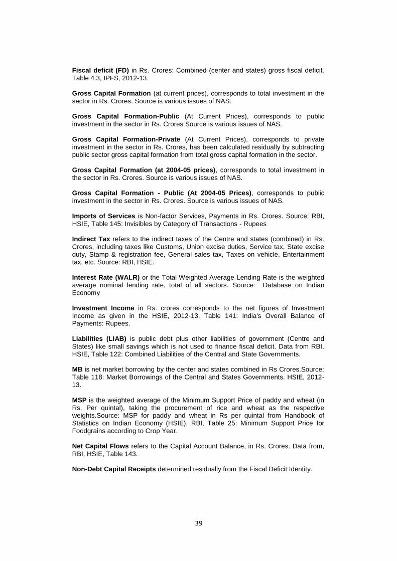
39
Fiscal deficit (FD) in Rs. Crores: Combined (center and states) gross fiscal deficit. Table 4.3, IPFS, 2012-13. Gross Capital Formation (at current prices), corresponds to total investment in the sector in Rs. Crores. Source is various issues of NAS. Gross Capital Formation-Public (At Current Prices), corresponds to public investment in the sector in Rs. Crores Source is various issues of NAS. Gross Capital Formation-Private (At Current Prices), corresponds to private investment in the sector in Rs. Crores, has been calculated residually by subtracting public sector gross capital formation from total gross capital formation in the sector. Gross Capital Formation (at 2004-05 prices), corresponds to total investment in the sector in Rs. Crores. Source is various issues of NAS. Gross Capital Formation - Public (At 2004-05 Prices), corresponds to public investment in the sector in Rs. Crores. Source is various issues of NAS. Imports of Services is Non-factor Services, Payments in Rs. Crores. Source: RBI, HSIE, Table 145: Invisibles by Category of Transactions - Rupees Indirect Tax refers to the indirect taxes of the Centre and states (combined) in Rs. Crores, including taxes like Customs, Union excise duties, Service tax, State excise duty, Stamp & registration fee, General sales tax, Taxes on vehicle, Entertainment tax, etc. Source: RBI, HSIE. Interest Rate (WALR) or the Total Weighted Average Lending Rate is the weighted average nominal lending rate, total of all sectors. Source: Database on Indian Economy Investment Income in Rs. crores corresponds to the net figures of Investment Income as given in the HSIE, 2012-13, Table 141: India's Overall Balance of Payments: Rupees. Liabilities (LIAB) is public debt plus other liabilities of government (Centre and States) like small savings which is not used to finance fiscal deficit. Data from RBI, HSIE, Table 122: Combined Liabilities of the Central and State Governments. MB is net market borrowing by the center and states combined in Rs Crores.Source: Table 118: Market Borrowings of the Central and States Governments. HSIE, 2012-13. MSP is the weighted average of the Minimum Support Price of paddy and wheat (in Rs. Per quintal), taking the procurement of rice and wheat as the respective weights.Source: MSP for paddy and wheat in Rs per quintal from Handbook of Statistics on Indian Economy (HSIE), RBI, Table 25: Minimum Support Price for Foodgrains according to Crop Year. Net Capital Flows refers to the Capital Account Balance, in Rs. Crores. Data from, RBI, HSIE, Table 143. Non-Debt Capital Receipts determined residually from the Fiscal Deficit Identity.
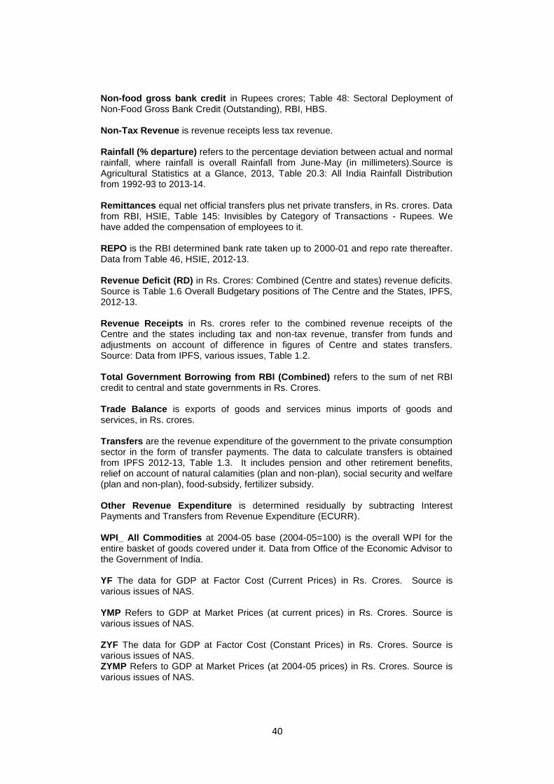
40
Non-food gross bank credit in Rupees crores; Table 48: Sectoral Deployment of Non-Food Gross Bank Credit (Outstanding), RBI, HBS. Non-Tax Revenue is revenue receipts less tax revenue. Rainfall (% departure) refers to the percentage deviation between actual and normal rainfall, where rainfall is overall Rainfall from June-May (in millimeters).Source is Agricultural Statistics at a Glance, 2013, Table 20.3: All India Rainfall Distribution from 1992-93 to 2013-14. Remittances equal net official transfers plus net private transfers, in Rs. crores. Data from RBI, HSIE, Table 145: Invisibles by Category of Transactions - Rupees. We have added the compensation of employees to it. REPO is the RBI determined bank rate taken up to 2000-01 and repo rate thereafter. Data from Table 46, HSIE, 2012-13. Revenue Deficit (RD) in Rs. Crores: Combined (Centre and states) revenue deficits. Source is Table 1.6 Overall Budgetary positions of The Centre and the States, IPFS, 2012-13. Revenue Receipts in Rs. crores refer to the combined revenue receipts of the Centre and the states including tax and non-tax revenue, transfer from funds and adjustments on account of difference in figures of Centre and states transfers. Source: Data from IPFS, various issues, Table 1.2. Total Government Borrowing from RBI (Combined) refers to the sum of net RBI credit to central and state governments in Rs. Crores. Trade Balance is exports of goods and services minus imports of goods and services, in Rs. crores. Transfers are the revenue expenditure of the government to the private consumption sector in the form of transfer payments. The data to calculate transfers is obtained from IPFS 2012-13, Table 1.3. It includes pension and other retirement benefits, relief on account of natural calamities (plan and non-plan), social security and welfare (plan and non-plan), food-subsidy, fertilizer subsidy. Other Revenue Expenditure is determined residually by subtracting Interest Payments and Transfers from Revenue Expenditure (ECURR). WPI_ All Commodities at 2004-05 base (2004-05=100) is the overall WPI for the entire basket of goods covered under it. Data from Office of the Economic Advisor to the Government of India. YF The data for GDP at Factor Cost (Current Prices) in Rs. Crores. Source is various issues of NAS. YMP Refers to GDP at Market Prices (at current prices) in Rs. Crores. Source is various issues of NAS. ZYF The data for GDP at Factor Cost (Constant Prices) in Rs. Crores. Source is various issues of NAS. ZYMP Refers to GDP at Market Prices (at 2004-05 prices) in Rs. Crores. Source is various issues of NAS.
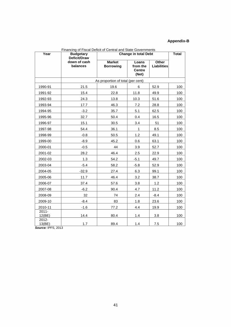
41
Appendix-B
Financing of Fiscal Deficit of Central and State Governments
Year Budgetary Deficit/Draw
down of cash balances
Change in total Debt
Total
Market Borrowing
Loans from the Centre (Net)
Other Liabilities
As proportion of total (per cent)
1990-91 21.5 19.6 6 52.9 100
1991-92 15.4 22.8 11.8 49.9 100
1992-93 24.3 13.8 10.3 51.6 100
1993-94 17.7 46.3 7.2 28.8 100
1994-95 -3.2 35.7 5.1 62.5 100
1995-96 32.7 50.4 0.4 16.5 100
1996-97 15.1 30.5 3.4 51 100
1997-98 54.4 36.1 1 8.5 100
1998-99 -0.8 50.5 1.2 49.1 100
1999-00 -8.9 45.2 0.6 63.1 100
2000-01 -0.5 44 3.9 52.7 100
2001-02 28.2 46.4 2.5 22.9 100
2002-03 1.3 54.2 -5.1 49.7 100
2003-04 -5.4 58.2 -5.8 52.9 100
2004-05 -32.9 27.4 6.3 99.1 100
2005-06 11.7 46.4 3.2 38.7 100
2006-07 37.4 57.6 3.8 1.2 100
2007-08 -6.2 90.4 4.7 11.2 100
2008-09 32 74 2.4 -8.4 100
2009-10 -8.4 83 1.8 23.6 100
2010-11 -1.6 77.2 4.4 19.9 100
2011-12(BE) 14.4 80.4 1.4 3.8 100
2012-13(BE) 1.7 89.4 1.4 7.5 100
Source: IPFS, 2013

42
Figure No.1: Share of Public Investment in Total Sectoral Investment (Public and Private)
Source: NAS, 2005 and 2013.
Figure No.2: Sectoral Capital-Output Ratio (HP-Trend)
Source: NAS, 2013.

43
Figure No.3: Sector-wise Share in Public Capital Expenditure
Source: NAS, 2013.
Figure No.4: Revenue Deficit and Capital Expenditure as % GDP
Source: IPFS, various issues.
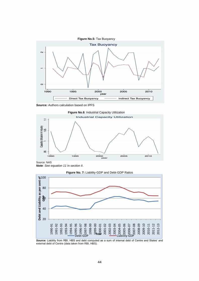
44
Figure No.5: Tax Buoyancy
Source: Authors calculation based on IPFS
Figure No.6: Industrial Capacity Utilization
Source: NAS
Note: See equation 11 in section II.
Figure No. 7: Liability-GDP and Debt-GDP Ratios
Source: Liability from RBI, HBS and debt computed as a sum of internal debt of Centre and States‟ and external debt of Centre (data taken from RBI, HBS).
20
40
60
80
100
19
90
-91
19
91
-92
19
92
-93
19
93
-94
19
94
-95
19
95
-96
19
96
-97
19
97
-98
19
98
-99
19
99
-00
20
00
-01
20
01
-02
20
02
-03
20
03
-04
20
04
-05
20
05
-06
20
06
-07
20
07
-08
20
08
-09
20
09
-10
20
10
-11
20
11
-12
20
12
-13
De
bt
and
Lia
bili
ty a
s p
er
cen
t o
f G
DP
Year Debt-GDP Liability-GDP
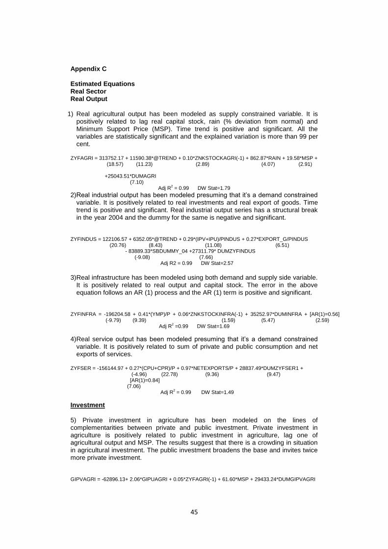
45
Appendix C Estimated Equations Real Sector Real Output
1) Real agricultural output has been modeled as supply constrained variable. It is positively related to lag real capital stock, rain (% deviation from normal) and Minimum Support Price (MSP). Time trend is positive and significant. All the variables are statistically significant and the explained variation is more than 99 per cent.
ZYFAGRI = 313752.17 + 11590.38*@TREND + 0.10*ZNKSTOCKAGRI(-1) + 862.87*RAIN + 19.58*MSP + (18.57) (11.23) (2.89) (4.07) (2.91) +25043.51*DUMAGRI (7.10)
Adj R2 = 0.99 DW Stat=1.79
2) Real industrial output has been modeled presuming that it‟s a demand constrained variable. It is positively related to real investments and real export of goods. Time trend is positive and significant. Real industrial output series has a structural break in the year 2004 and the dummy for the same is negative and significant.
ZYFINDUS = 122106.57 + 6352.05*@TREND + 0.29*(IPV+IPU)/PINDUS + 0.27*EXPORT_G/PINDUS (20.76) (8.43) (11.08) (6.51) - 83889.33*SBDUMMY_04 +27311.79* DUMZYFINDUS (-9.08) (7.66) Adj R2 = 0.99 DW Stat=2.57
3) Real infrastructure has been modeled using both demand and supply side variable.
It is positively related to real output and capital stock. The error in the above equation follows an AR (1) process and the AR (1) term is positive and significant.
ZYFINFRA = -196204.58 + 0.41*(YMP)/P + 0.06*ZNKSTOCKINFRA(-1) + 35252.97*DUMINFRA + [AR(1)=0.56] (-9.79) (9.39) (1.59) (5.47) (2.59)
Adj R2 =0.99 DW Stat=1.69
4) Real service output has been modeled presuming that it‟s a demand constrained variable. It is positively related to sum of private and public consumption and net exports of services.
ZYFSER = -156144.97 + 0.27*(CPU+CPR)/P + 0.97*NETEXPORTS/P + 28837.49*DUMZYFSER1 + (-4.96) (22.78) (9.36) (9.47) [AR(1)=0.84] (7.06) Adj R
2 = 0.99 DW Stat=1.49
Investment 5) Private investment in agriculture has been modeled on the lines of complementarities between private and public investment. Private investment in agriculture is positively related to public investment in agriculture, lag one of agricultural output and MSP. The results suggest that there is a crowding in situation in agricultural investment. The public investment broadens the base and invites twice more private investment.
GIPVAGRI = -62896.13+ 2.06*GIPUAGRI + 0.05*ZYFAGRI(-1) + 61.60*MSP + 29433.24*DUMGIPVAGRI
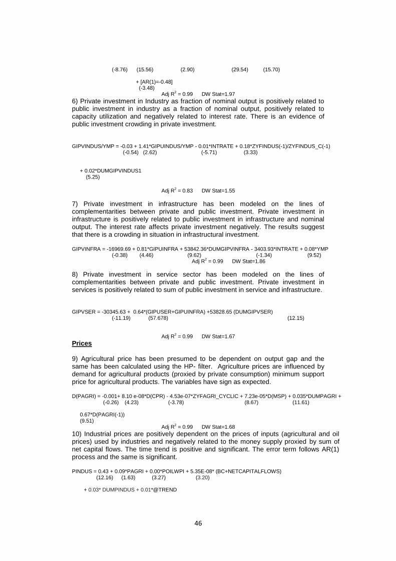
46
(-8.76) (15.56) (2.90) (29.54) (15.70) + [AR(1)=-0.48] (-3.48)
Adj R2 = 0.99 DW Stat=1.97
6) Private investment in Industry as fraction of nominal output is positively related to public investment in industry as a fraction of nominal output, positively related to capacity utilization and negatively related to interest rate. There is an evidence of public investment crowding in private investment. GIPVINDUS/YMP = -0.03 + 1.41*GIPUINDUS/YMP - 0.01*INTRATE + 0.18*ZYFINDUS(-1)/ZYFINDUS_C(-1) (-0.54) (2.62) (-5.71) (3.33) + 0.02*DUMGIPVINDUS1 (5.25)
Adj R
2 = 0.83 DW Stat=1.55
7) Private investment in infrastructure has been modeled on the lines of complementarities between private and public investment. Private investment in infrastructure is positively related to public investment in infrastructure and nominal output. The interest rate affects private investment negatively. The results suggest that there is a crowding in situation in infrastructural investment. GIPVINFRA = -16969.69 + 0.81*GIPUINFRA + 53842.36*DUMGIPVINFRA - 3403.93*INTRATE + 0.08*YMP (-0.38) (4.46) (9.62) (-1.34) (9.52)
Adj R2 = 0.99 DW Stat=1.86
8) Private investment in service sector has been modeled on the lines of complementarities between private and public investment. Private investment in services is positively related to sum of public investment in service and infrastructure.
GIPVSER = -30345.63 + 0.64*(GIPUSER+GIPUINFRA) +53828.65 (DUMGIPVSER) (-11.19) (57.678) (12.15)
Adj R2 = 0.99 DW Stat=1.67
Prices 9) Agricultural price has been presumed to be dependent on output gap and the same has been calculated using the HP- filter. Agriculture prices are influenced by demand for agricultural products (proxied by private consumption) minimum support price for agricultural products. The variables have sign as expected. D(PAGRI) = -0.001+ 8.10 e-08*D(CPR) - 4.53e-07*ZYFAGRI_CYCLIC + 7.23e-05*D(MSP) + 0.035*DUMPAGRI + (-0.26) (4.23) (-3.78) (8.67) (11.61) 0.67*D(PAGRI(-1)) (9.51)
Adj R2 = 0.99 DW Stat=1.68
10) Industrial prices are positively dependent on the prices of inputs (agricultural and oil prices) used by industries and negatively related to the money supply proxied by sum of net capital flows. The time trend is positive and significant. The error term follows AR(1) process and the same is significant. PINDUS = 0.43 + 0.09*PAGRI + 0.00*POILWPI + 5.35E-08* (BC+NETCAPITALFLOWS) (12.16) (1.63) (3.27) (3.20) + 0.03* DUMPINDUS + 0.01*@TREND
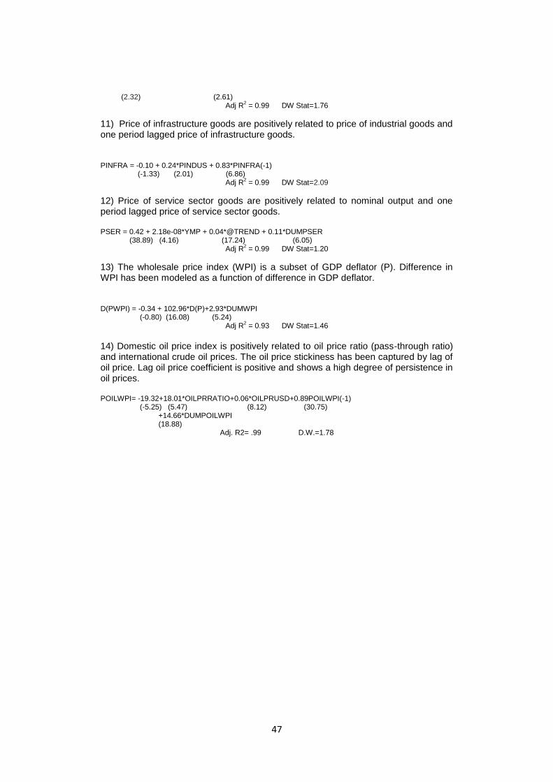
47
(2.32) (2.61) Adj R
2 = 0.99 DW Stat=1.76
11) Price of infrastructure goods are positively related to price of industrial goods and one period lagged price of infrastructure goods.
PINFRA = -0.10 + 0.24*PINDUS + 0.83*PINFRA(-1) (-1.33) (2.01) (6.86)
Adj R2 = 0.99 DW Stat=2.09
12) Price of service sector goods are positively related to nominal output and one period lagged price of service sector goods. PSER = 0.42 + 2.18e-08*YMP + 0.04*@TREND + 0.11*DUMPSER (38.89) (4.16) (17.24) (6.05)
Adj R2 = 0.99 DW Stat=1.20
13) The wholesale price index (WPI) is a subset of GDP deflator (P). Difference in WPI has been modeled as a function of difference in GDP deflator.
D(PWPI) = -0.34 + 102.96*D(P)+2.93*DUMWPI (-0.80) (16.08) (5.24)
Adj R2 = 0.93 DW Stat=1.46
14) Domestic oil price index is positively related to oil price ratio (pass-through ratio) and international crude oil prices. The oil price stickiness has been captured by lag of oil price. Lag oil price coefficient is positive and shows a high degree of persistence in oil prices.
POILWPI= -19.32+18.01*OILPRRATIO+0.06*OILPRUSD+0.89POILWPI(-1) (-5.25) (5.47) (8.12) (30.75) +14.66*DUMPOILWPI (18.88)
Adj. R2= .99 D.W.=1.78
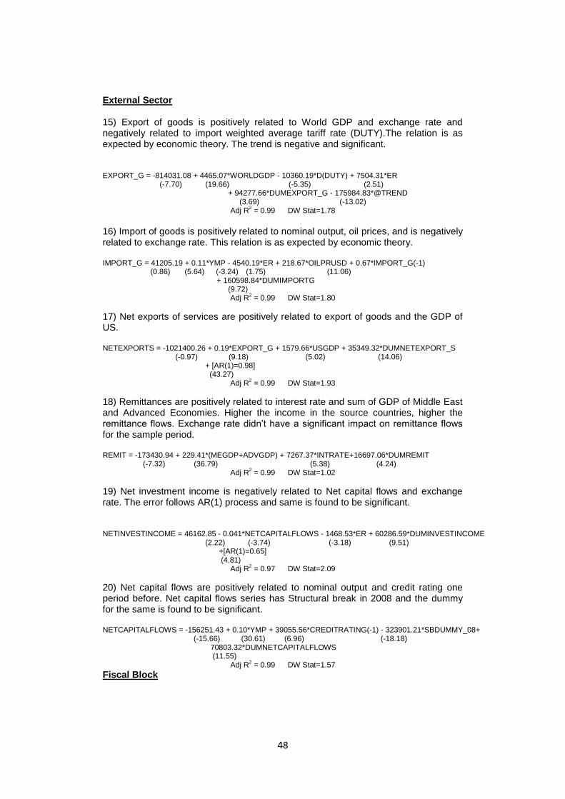
48
External Sector 15) Export of goods is positively related to World GDP and exchange rate and negatively related to import weighted average tariff rate (DUTY).The relation is as expected by economic theory. The trend is negative and significant. EXPORT_G = -814031.08 + 4465.07*WORLDGDP - 10360.19*D(DUTY) + 7504.31*ER (-7.70) (19.66) (-5.35) (2.51) + 94277.66*DUMEXPORT_G - 175984.83*@TREND
(3.69) (-13.02) Adj R
2 = 0.99 DW Stat=1.78
16) Import of goods is positively related to nominal output, oil prices, and is negatively related to exchange rate. This relation is as expected by economic theory. IMPORT_G = 41205.19 + 0.11*YMP - 4540.19*ER + 218.67*OILPRUSD + 0.67*IMPORT_G(-1) (0.86) (5.64) (-3.24) (1.75) (11.06) + 160598.84*DUMIMPORTG (9.72)
Adj R2 = 0.99 DW Stat=1.80
17) Net exports of services are positively related to export of goods and the GDP of US. NETEXPORTS = -1021400.26 + 0.19*EXPORT_G + 1579.66*USGDP + 35349.32*DUMNETEXPORT_S (-0.97) (9.18) (5.02) (14.06) + [AR(1)=0.98] (43.27)
Adj R2 = 0.99 DW Stat=1.93
18) Remittances are positively related to interest rate and sum of GDP of Middle East and Advanced Economies. Higher the income in the source countries, higher the remittance flows. Exchange rate didn‟t have a significant impact on remittance flows for the sample period. REMIT = -173430.94 + 229.41*(MEGDP+ADVGDP) + 7267.37*INTRATE+16697.06*DUMREMIT (-7.32) (36.79) (5.38) (4.24)
Adj R2 = 0.99 DW Stat=1.02
19) Net investment income is negatively related to Net capital flows and exchange rate. The error follows AR(1) process and same is found to be significant.
NETINVESTINCOME = 46162.85 - 0.041*NETCAPITALFLOWS - 1468.53*ER + 60286.59*DUMINVESTINCOME (2.22) (-3.74) (-3.18) (9.51) +[AR(1)=0.65] (4.81)
Adj R2 = 0.97 DW Stat=2.09
20) Net capital flows are positively related to nominal output and credit rating one period before. Net capital flows series has Structural break in 2008 and the dummy for the same is found to be significant. NETCAPITALFLOWS = -156251.43 + 0.10*YMP + 39055.56*CREDITRATING(-1) - 323901.21*SBDUMMY_08+ (-15.66) (30.61) (6.96) (-18.18) 70803.32*DUMNETCAPITALFLOWS (11.55)
Adj R2 = 0.99 DW Stat=1.57
Fiscal Block
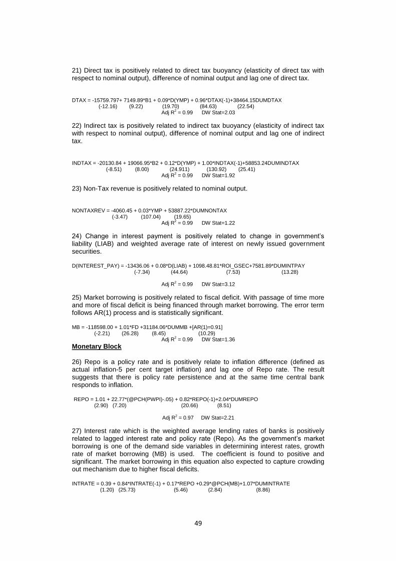
49
21) Direct tax is positively related to direct tax buoyancy (elasticity of direct tax with respect to nominal output), difference of nominal output and lag one of direct tax.
DTAX = -15759.797+ 7149.89*B1 + 0.09*D(YMP) + 0.96*DTAX(-1)+38464.15DUMDTAX (-12.16) (9.22) (19.70) (84.63) (22.54)
Adj R2 = 0.99 DW Stat=2.03
22) Indirect tax is positively related to indirect tax buoyancy (elasticity of indirect tax with respect to nominal output), difference of nominal output and lag one of indirect tax.
INDTAX = -20130.84 + 19066.95*B2 + 0.12*D(YMP) + 1.00*INDTAX(-1)+58853.24DUMINDTAX (-8.51) (8.00) (24.911) (130.92) (25.41)
Adj R2 = 0.99 DW Stat=1.92
23) Non-Tax revenue is positively related to nominal output.
NONTAXREV = -4060.45 + 0.03*YMP + 53887.22*DUMNONTAX (-3.47) (107.04) (19.65)
Adj R2 = 0.99 DW Stat=1.22
24) Change in interest payment is positively related to change in government‟s liability (LIAB) and weighted average rate of interest on newly issued government securities.
D(INTEREST_PAY) = -13436.06 + 0.08*D(LIAB) + 1098.48.81*ROI_GSEC+7581.89*DUMINTPAY (-7.34) (44.64) (7.53) (13.28)
Adj R
2 = 0.99 DW Stat=3.12
25) Market borrowing is positively related to fiscal deficit. With passage of time more and more of fiscal deficit is being financed through market borrowing. The error term follows AR(1) process and is statistically significant. MB = -118598.00 + 1.01*FD +31184.06*DUMMB +[AR(1)=0.91] (-2.21) (26.28) (8.45) (10.29)
Adj R2 = 0.99 DW Stat=1.36
Monetary Block 26) Repo is a policy rate and is positively relate to inflation difference (defined as actual inflation-5 per cent target inflation) and lag one of Repo rate. The result suggests that there is policy rate persistence and at the same time central bank responds to inflation.
REPO = 1.01 + 22.77*(@PCH(PWPI)-.05) + 0.82*REPO(-1)+2.04*DUMREPO (2.90) (7.20) (20.66) (8.51)
Adj R
2 = 0.97 DW Stat=2.21
27) Interest rate which is the weighted average lending rates of banks is positively related to lagged interest rate and policy rate (Repo). As the government‟s market borrowing is one of the demand side variables in determining interest rates, growth rate of market borrowing (MB) is used. The coefficient is found to positive and significant. The market borrowing in this equation also expected to capture crowding out mechanism due to higher fiscal deficits.
INTRATE = 0.39 + 0.84*INTRATE(-1) + 0.17*REPO +0.29*@PCH(MB)+1.07*DUMINTRATE (1.20) (25.73) (5.46) (2.84) (8.86)
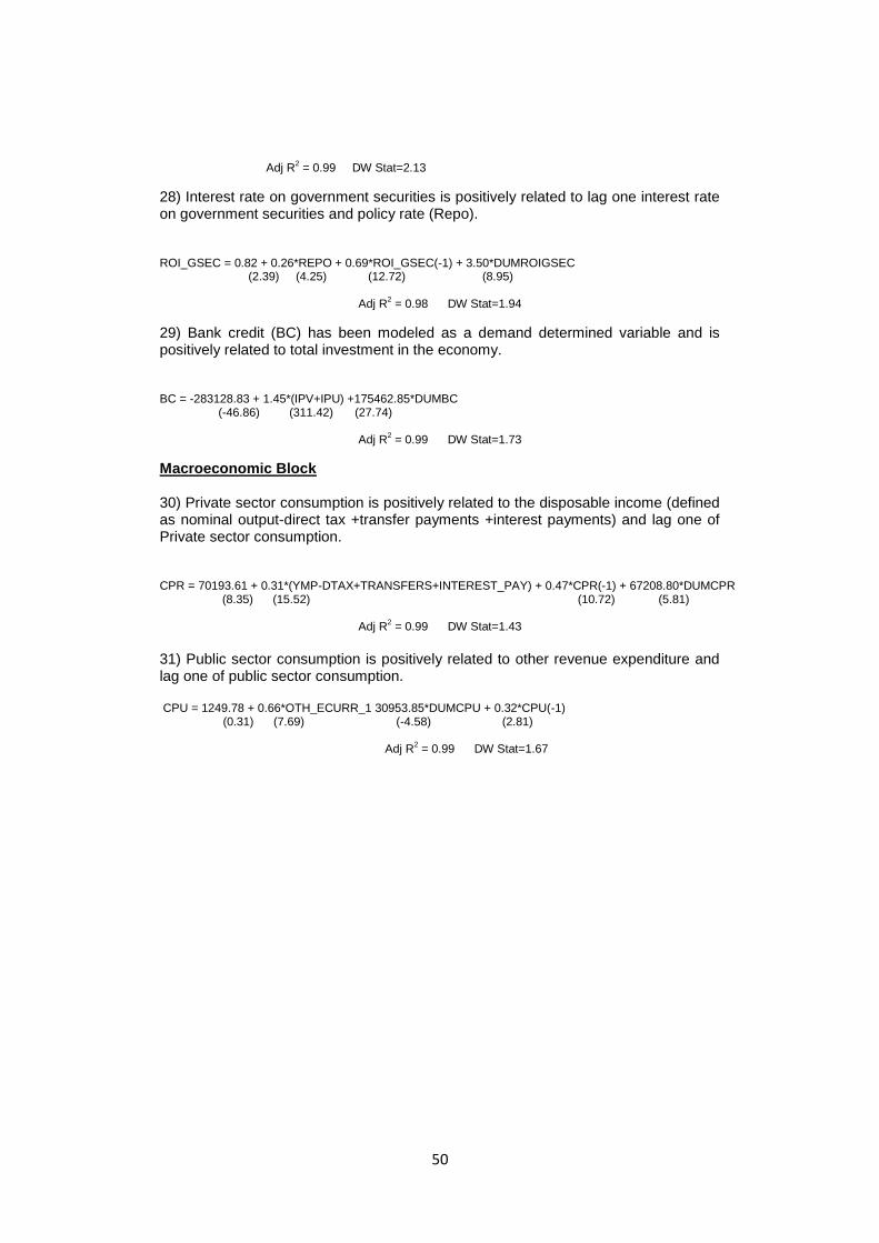
50
Adj R
2 = 0.99 DW Stat=2.13
28) Interest rate on government securities is positively related to lag one interest rate on government securities and policy rate (Repo).
ROI_GSEC = 0.82 + 0.26*REPO + 0.69*ROI_GSEC(-1) + 3.50*DUMROIGSEC (2.39) (4.25) (12.72) (8.95)
Adj R
2 = 0.98 DW Stat=1.94
29) Bank credit (BC) has been modeled as a demand determined variable and is positively related to total investment in the economy.
BC = -283128.83 + 1.45*(IPV+IPU) +175462.85*DUMBC (-46.86) (311.42) (27.74)
Adj R
2 = 0.99 DW Stat=1.73
Macroeconomic Block 30) Private sector consumption is positively related to the disposable income (defined as nominal output-direct tax +transfer payments +interest payments) and lag one of Private sector consumption.
CPR = 70193.61 + 0.31*(YMP-DTAX+TRANSFERS+INTEREST_PAY) + 0.47*CPR(-1) + 67208.80*DUMCPR (8.35) (15.52) (10.72) (5.81)
Adj R2 = 0.99 DW Stat=1.43
31) Public sector consumption is positively related to other revenue expenditure and lag one of public sector consumption. CPU = 1249.78 + 0.66*OTH_ECURR_1 30953.85*DUMCPU + 0.32*CPU(-1)
(0.31) (7.69) (-4.58) (2.81)
Adj R2 = 0.99 DW Stat=1.67