Sains Malaysiana 40(8)(2011): 927–935

Tail Dependence Estimate in Financial Market Risk Management: Clayton-Gumbel Copula Approach

(Nilai Kebersandaran Ekor Bagi Anggaran Dalam Pengurusan Risiko Pasaran Kewangan: Pendekatan Clayton-Gumbel Copula)

A. SHAMIRI., N.A. HAMZAH & A. PIRMORADIAN

ABSTRACT

This paper focuses on measuring risk due to extreme events going beyond the multivariate normal distribution of joint returns. The concept of tail dependence has been found useful as a tool to describe dependence between extreme data in finance. Specifically, we adopted a multivariate Copula-EGARCH approach in order to investigate the presence of conditional dependence between international financial markets. In addition, we proposed a mixed Clayton-Gumbel copula with estimators for measuring both, the upper and lower tail dependence. The results showed significant dependence for Singapore and Malaysia as well as for Singapore and US, while the dependence for Malaysia and US was relatively weak.

Keywords: Copulas; EGARCH model; risk measures; tail dependence

ABSTRAK

Kajian ini menumpu kepada pengukuran risiko yang disebabkan oleh kejadian ekstrim yang berlaku di luar batasan taburan multivariat normal bagi pulangan bercantum. Konsep kebersandaran ekor telah didapati berguna sebagai alat bagi menerangkan kebersandaran di kalangan data ekstrim dalam kewangan. Secara spesifik, kami mengadaptasi pendekatan multivariate Copula-EGARCH untuk mengkaji kewujudan kebersandaran bersyarat antara pasaran kewangan antarabangsa. Kami juga mencadangkan campuran copula Clayton-Gumbel dengan penganggar bagi mengukur kedua-dua had atas dan bawah ekor kebersandaran. Keputusan kajian ini menunjukkan kebersandaran yang signifikan antara Singapura-Malaysia serta Singapura-Amerika Syarikat, manakala kebersandaran untuk Malaysia-Amerika Syarikat adalah lemah secara relatif.

Kata kunci: Copula; kebersandaran ekor; model EGARCH; ukuran risiko

INTRODUCTION

In financial risk management, a risk is indicative of any uncertainty that might trigger losses. In portfolio management for example, the risk with a variety of asset returns posed a challenge in trying to attain a complete picture of these risks joint distribution and the respective model. The ability of such risk measures is important as it will assist financial managers on how best to (1) position one’s investment and (2) enhance one’s financial risk protection. Capturing comovement between financial asset returns with linear correlation has been the staple approach in modern finance since the birth of Harry Markowitz’s theory. Linear correlation is the appropriate measure of dependence if asset returns follow a multivariate normal (elliptical) distribution. However, the statistical analysis of the distribution of individual asset returns frequently finds fat tails, skewness and other non-normal features which leads to underestimation of this measure (Ang & Bekaert 2002; Ang & Chen 2002; Bae et al. 2003; Longin & Solnik 2001). If the normal distribution is inadequate, then it is not clear how to appropriately measure the dependence between multiple asset returns.

It is well known that in financial markets large changes tend to be followed by larger changes and small changes tend to be followed by smaller changes. In other words, the financial markets are sometimes more volatile and sometimes less. A large number of researchers have also found ample evidence that conditional variance of financial time series are interacting and that the cross market correlation coefficients are conditional on market volatility. The estimates of this correlation tend to increase, particularly during crises when markets are more volatile (Engle 2002). This correlation is not related directly to market volatility but it increases in bear markets rather than in bull markets. Besides that, in order to evaluate the risk due to extreme events, it is necessary to measure the tail dependence that is concordance between less probable values of variables. This suggests a significant dependence in the tails of the joint distribution of asset returns to be analyzed with a possibly asymmetric model. Fortunately, the theory of copulas provides a flexible methodology for the general modelling of multivariate dependence. In general, a copula is a function that links

928

n-dimensional distribution function (marginals) to its one dimensional margins and is itself a continuous distribution function which characterizes the model’s dependence structure. Since the copula methods provide a way to isolate the dependence structure of the portfolio from the individual margins of the assets, flexibility in modelling the portfolio is provided. A specific copula is chosen and this depends on the composition of the portfolio. Empirical studies (Engle 2002; Hamo et al. 1990; Hong 2001) showed that market volatility increases in bear market rather than in bull market and this implies that the dependence structure should allow for tail dependency among assets. However, much less attention has been paid to the possibility of asymmetric dependence between financial markets. In this paper, instead of relying on symmetric copula models in measuring dependence we may extend the case to asymmetric copulas, allowing for both positive and negative effects to take place. It is to our knowledge, the first attempt to investigate the dependence structures between international financial markets, in the context of mixed Clayton-Gumbel copulas. We find significant evidence of dependence structure between the US and Singapore as well as Singapore and Malaysia, along with some asymmetry. As an evidence of asymmetric dependence, we find that the magnitude of the lower tail dependence is much greater than the upper tail dependence, suggesting two financial markets exhibit greater dependence during market downturns than market upturns. On the contrary, the tail dependence coefficient for the bivariate series KLCI-SP500 exhibit weak relationship among both series, which may be due capital control in Malaysia. The aims of this paper were to investigate the presence of conditional tail dependence between international markets and measure the dependence using a conditional Copula-EGARCH approach (Jondeau & Rockinger 2006). The Copula-EGARCH model can capture the dependence in the uncorrelated errors ignored by all existing EGARCH models. Moreover, a copula function has been exploited to describe the whole dependence structure that characterizes the relationship between variables. To allow for an asymmetric impact of positive and negative shocks on the conditional volatility (leverage effect), the EGARCH model is employed; for every EGARCH model, the corresponding Copula-EGARCH model can be constructed. In the paper we analyse some bivariate Archimedean copula functions characterized by a different degree of concordance between extreme events. The reminder of this paper is organized as follows: next section introduces the concepts of copula and its estimation methods, with a special emphasis on introducing a new copula model. Methods of marginal models are described in the Marginal Models section. This is followed by empirical application sections and Conclusion which contains some concluding remarks.

COPULA

COPULA AND DEPENDENCy

Although a normal distribution is easy to use for measuring dependency, it is generally inconsistent in the presence of asymmetry and excess kurtosis which usually arise in financial data (Abu & Shamiri 2007; Abu et al. 2009). In this paper, we used the recently popular copulas to construct uncorrelated dependent errors. The principle characteristic of a copula function is its ability to decompose the joint distribution into two parts: marginal distributions and dependence structure. Different dependence structures can combine the same marginal distributions into different joint distributions. Similarly, different marginal distributions under the same dependence structure can also lead to different joint distributions.

Definition (Copula): A function C:[0,1]2 → [0,1] is a copula if it satisfies (i) C(u1, u2) = 0 for u1 = 0 or u2 = 0 (ii) C(u1,1) = u1,C(u2,1) = u2 for all u1 and u2 in the unit interval [0,1]; and (iii) (–1)i+j C(u1i,u2,j) ≥ 0 for all (u1,u2,j) in [0.1] with u1,1 < u1,2 and u2,1 < u2,2. The relationship between a copula and joint distribution function is illuminated by Sklar’s (1959) theorem. Sklar’s theorem shows that for continuous multivariate distributions the univariate margins can be separated from the dependence structure which is completely captured by a copula function.

Sklar’s Theorem: Let F12(.) be a joint distribution function with marginal distribution function Fi(.) for i = 1,2. Then there exists a copula function C, such as that for all x1, x2 in ,

F12(x1,x2) = C(F1(x1), F2(x2)) (1)

Conversely, if C is a copula and Fi(.) are marginal distribution functions, then F12(.) defined above is a joint distribution with margins Fi(.).

Corollary 1: Let denote the generalized inverses of the uniform marginal distribution function u1, u2, then for every (u1,u2) in the unit n-cube, there exists a unique copula C:[0,1]2 such that F12 = C(u1,u2) where = inf[xi : Fi(xi) > ui]; for i = 1,2. Given the copula density is defined as:

(2)

Then using the chain rule, the joint density may be recovered using

(3)

929

The above result showed that it is always possible to specify a bivariate density by specifying the marginal densities and a copula density. In other words, this means that the copula has all the information about dependence structure. Some of the copula properties such as being invariant to strictly increasing transformation of the random variables and the ability to measure the concordance between random variables are indeed very useful in the study of dependence. Therefore measuring tail dependence that is concordance between less probable values of variables, which is also a property of copula, has a great importance in the study of financial risk management. In a bivariate context, let Fi(.), i = 1,2, be the marginal distribution functions, X1, X2 are the residuals generated from equation (27) and let u be a threshold value. The upper tail coefficient, λU, is then defined as the limit when u tends to one, of the probability that the distribution function of the variable X1 exceeds u, given that the corresponding function for X2 exceeds u,

(4)

Since λU ∈ (0,1], we can say that for λU ∈ (0,1], X1 and X2 are asymptotically dependent on the upper tail; and when if λU = 0, X1 and X2 are asymptotically independent. It is also easy to show in terms of copula function that

(5)

The concept of lower tail dependence can be defined in a similar way. Let Fi(.), i = 1, 2, be the marginal distribution functions of two variables, X1, X2 and let u be a threshold value, then λL, is defined as

(6)

In terms of copula function, the lower tail dependence takes the form,

(7)

Kendall’s tau is a measure of concordance between random variables (X1, X2) that measures the difference of probabilities between concordant and discordant random variables

τ = P[X1– )(X2– )>0]–P[X1– )(X2– )<0] (8)

where is a second independent pair with the same distribution as (X1, X2).

However, it is possible to express Kendall’s tau in term of the copula (Nelsen 2006; Embrechts et. al. 2002) that the Kendall’s tau τ correlation depends only on the copula C (and not on the marginal distributions of X1 and X2) and is given by

(9)

As a measure of concordance based on copulas, which means that it is invariant to increasing transformations of its arguments, Kendall’s tau can capture nonlinear dependences that were not possible to measure with linear correlation. The Gumbel and Clayton copulas may be used to represent the dependence structure implicit in a multivariate distribution, because of their properties, particularly in the context of modelling multivariate financial return data (for example daily relative or logarithmic price changes on number stocks). The Gumbel and Clayton copulas belong to the Archimedean copula family. The family of Archimedean copulas (Cherubini et al. 2004; Joe 1997) can be built starting from the definition of a generator function Φ : I ∈ R+, which is continuous, decreasing and that Φ(1) = 0. Specifically, let Φ be a generator, then an Archimedean copula CA can be expressed as

CA(u1,u2) = Φ–1(Φ(u1) + Φ(u2)). (10)

The Archimedean copulas share the important features of symmetry and associativity. The Clayton copula is given by

CC(u1,u2) = [ + –1]–1/θ (11)

The copula has a generator, Φ(t) = (t–θ–1) while

Φ–1(t) = (1+t)–1/θ. When θ > 0, it is completely monotonic. With θ → 0, CC(u1,u2) = u1u2 and when θ → ∞ the upper Frechet-Hoefding bound is attained. Therefore upper tail dependency is equal to zero and the lower tail dependency is λL = 2–(1/θ). Kendall’s tau of this copula can be defined as

The Gumbel copula which belongs to the extreme values (EV) family (Gumbel, 1960) is expressed as

(12)

The generator Φ(t) = (-ln t)ζ while Φ–1(t) = exp(–t1/ζ). The parameter ζ controls the strength of dependence; ζ =

1, implies CG(u1,u2) = u1u2,which reflects no dependency; when ζ = +∞, is indicative of a perfect dependence. Here, the lower tail dependence is zero, λL = 0, and upper tail dependence takes the form λU = 2–2–(1/ζ). The corresponding Kendall’s tau can be defined as τ = 1–

In this paper, we bring together what is known about the Archimedean copula Clayton and Gumbel, particularly with regard to its extremal properties, and present some extensions of the CC and CG copulas that overcome their limitations through extreme value theory. Clearly, the Archimedean copulas (CC and CG) introduce above cannot explain all the tail behaviour observed on financial markets. CC, displays only negative (lower) tail dependence, = 2–1/θ, while CG which is probably the most common EV copula exhibits only positive (upper) tail

930

dependency, = 2–2–1/ζ. To overcome to this problem, the Joe- Clayton copula has been introduced. The Joe-Clayton copula belongs to the family BB7 (Joe 1997) and is expressed as

(13)

where and

Although, the Joe-Clayton copula shows both the negative (lower) and positive (upper) tail dependence, respectively = 2–1/θ and = 2–21/k respectively, it does not count for extreme events. To solve this difficulty a new combination of CC and CG copulas will be introduced. The new copula introduced here, arises from the fact that any combination of two Archimedean copulas is an Archimedean copula (Nelsen 2006). Thus, in order to obtain copulas which have upper and lower tail dependence that are not necessarily symmetrical, we employ a convex linear combination of these two copulas. That is, for π ∈ [0,1] and two Archimedean copulas, namely, Clayton CC and Gumbel CG, we define

CCG(u1,u2) = πCC (u1,u2)+(1-π)CG(u1,u2) (14)

We denote (14) as a mixed Clayton-Gumbel (CG) copula. The properties of these copulas can be derived from those of CC and CG. The upper and lower tail dependence of the mixed Claytom-Gumbel are given by

and

respectively, of the form,

= (1 – π) (15)

and

= (16)

Likewise, the kendall’s τ of the copula CCG defined in (14) can be expressed as,

τCG = π2τC + (1 – π)2 τG + 2π(1 – π)

[4�l2CC(u1,u2)dCG(u1,u2) –1]

= π2τC + (1–π)2τG + 2π(1 – π)

(17)

Equation (17) can also be expressed as functions of the parameters θ and ζ. Since θ and ζ are the respective parameters of CC and CG, (17) becomes – equation (18) – for π ≠ 0,1 where,

τCG = πθ/(θ + 2)+( 1– π)(1 – 1/ζ)+2π(1 – π) (18)

where

(19)

and

(20)

For a given τCG, , and π deduced from (18), the estimates of θ and ζ are obtained from (19) and (20). Here, the negative (lower) and positive (upper) tail dependence are given respectively by,

= π2–1/θ (21)

and

= (1 – π)(2 – 21/ζ). (22)

MAxIMUM LIKELIHOOD ESTIMATION

Consider a bivariate distribution F12 with margins distributions Fi, pdf f i and a copula with density c. Let α be the vector of marginal parameters of Fi and θ be the vector of copula parameters. The parameters of the joint density to be estimated is η = (α',θ')' . From (3) the log-likelihood function is then

(23)

and the exact maximum likelihood estimator (MLE) is defined as

= argη max l(η)

The numerical computation of the exact MLE may be difficult if there are many parameters in the marginal models and in the copula. Instead of maximizing the likelihood (23) as a function of η, the copula parameters θ may be estimated using a two-stage procedure proposed by Joe and Xu (1996) called the inference function for margins (IFM). Using IFM, the marginal distributions Fi are estimated. This could be done using parametric models (e.g., normal or student’s-t distribution), the empirical CDF, or a combination of an empirical CDF with an estimated generalized Pareto distribution for the tail. The marginal parameters α are estimated by

(24)

Based on the estimates , we next estimate the association parameters θ via

(25)

931

Under standard regularity conditions, the IFM estimators are consistent and asympotically normally distributed. In particular, Joe (1997) showed that the IFM estimate often nearly as efficient as the MLE estimate.

MARGINAL MODELS

The idea of using copula is to construct a bivariate distribution where we first need to make an assumption about each univariate marginal distribution, i.e. student-t distribution. For ease of exposition, we estimate asymmetric auto-regressive EGARCH (1, 1) model of Nelson (1991) for the time series of financial market returns. This model looks at the conditional variance and tries to accommodate for the asymmetric relation between financial market returns and volatility changes. Consider a d-dimensional time series sample of length T. For each univariate time series, we specify the marginal model,

(26)

εi,t|It–1~ t(v) for i ∈ {1,…,d}

ln (27)

where xi,t represents univariate market return series,

εi,t is the conditional mean of the series, vi is the error

component and assumed iid student-t distributed with iv degrees of freedom, denotes the variance, and

It–1 is the information set at time t – 1. The Ki as in (26) is determined by optimizing the Akaike Information Criterion (AIC). The EGARCH model in (27) differs from the standard GARCH model in two main aspects. First, it allows positive and negative shocks to have a different impact on volatility. Second, the EGARCH model allows large shocks to have a greater impact on volatility than the standard GARCH model. Note that when εi,t–1 is positive which is indicative of a bull market, the total effect of εi,t–1 is (1 + γi)| εi,t–1|; in contrast, when εi,t–1 is negative which suggests a bear market, the total effect of εi,t–1 is (1 – γi)| εi,t–1|. Bear markets usually have a larger impact on volatility, and the value of γi is expected to be negative. Using the probability integral transform we can infer for the univariate marginal distribution by forming the vectors ut = We will mainly focus on the Clayton, Gumbel, Joe-Clayton and the newly introduced Clayton-Gumbel copulas since the first three are frequently used in the literature for measuring general dependence, whereas the latter is good at modelling both, the upper and lower tail dependencies. These types of copula models will provide us with a full picture of dependence structures in financial markets.

EMPIRICAL APPLICATION

The objective of this section is to measure the tail dependence with a copula-EGARCH model. To elucidate

the effect of the distinct feature in the tail, we adopt the same normal marginal distribution so that the difference arises only from the copula density. We examine daily data of three stock indexes returns: the Strait Times Index (STI) of Singapore, the Kuala Lumpur Composite Index (KLCI) of Malaysia and Standard and Poor index (SP500) of USA for the period January 01st, 1998 through December 31st, 2008. The data sets collected from DataStream consist of daily closing price with a total of n = 2780 observations. In the database, the daily return Ri,t,i = 1,…,9 consisted of daily closing price Pi,t,

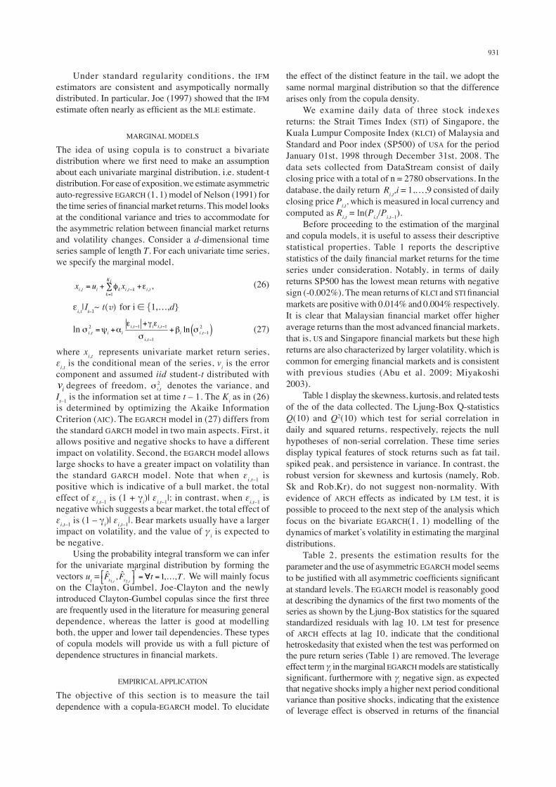
which is measured in local currency and computed as Ri,t = ln(Pi,t/Pi,t–1). Before proceeding to the estimation of the marginal and copula models, it is useful to assess their descriptive statistical properties. Table 1 reports the descriptive statistics of the daily financial market returns for the time series under consideration. Notably, in terms of daily returns SP500 has the lowest mean returns with negative sign (-0.002%). The mean returns of KLCI and STI financial markets are positive with 0.014% and 0.004% respectively. It is clear that Malaysian financial market offer higher average returns than the most advanced financial markets, that is, US and Singapore financial markets but these high returns are also characterized by larger volatility, which is common for emerging financial markets and is consistent with previous studies (Abu et al. 2009; Miyakoshi 2003). Table 1 display the skewness, kurtosis, and related tests of the of the data collected. The Ljung-Box Q-statistics Q(10) and Q2(10) which test for serial correlation in daily and squared returns, respectively, rejects the null hypotheses of non-serial correlation. These time series display typical features of stock returns such as fat tail, spiked peak, and persistence in variance. In contrast, the robust version for skewness and kurtosis (namely, Rob.Sk and Rob.Kr), do not suggest non-normality. With evidence of ARCH effects as indicated by LM test, it is possible to proceed to the next step of the analysis which focus on the bivariate EGARCH(1, 1) modelling of the dynamics of market’s volatility in estimating the marginal distributions. Table 2, presents the estimation results for the parameter and the use of asymmetric EGARCH model seems to be justified with all asymmetric coefficients significant at standard levels. The EGARCH model is reasonably good at describing the dynamics of the first two moments of the series as shown by the Ljung-Box statistics for the squared standardized residuals with lag 10. LM test for presence of ARCH effects at lag 10, indicate that the conditional hetroskedasity that existed when the test was performed on the pure return series (Table 1) are removed. The leverage effect term γi in the marginal EGARCH models are statistically significant, furthermore with γi negative sign, as expected that negative shocks imply a higher next period conditional variance than positive shocks, indicating that the existence of leverage effect is observed in returns of the financial

932

market series. Briefly, looking at the overall results, we can argue that EGARCH model adequately explains the data set under investigation. The marginal models seem to be able to capture the dynamics of the first and second moments of the returns of the financial time series. As mentioned earlier, the main aim of this paper is to investigate the presence of conditional tail dependence between international markets and to measure it using a new copula CCG approach. In this framework, we have used the Inference for the Margins (IFM) method, estimating into separate steps the margins and the copula parameters. Firstly, the marginal distributions of each stock index are independently estimated via maximum likelihood through an EGARCH model. After transforming the standardized residuals into uniform margins, we have estimated the above three copula functions for each pair of index stock returns.

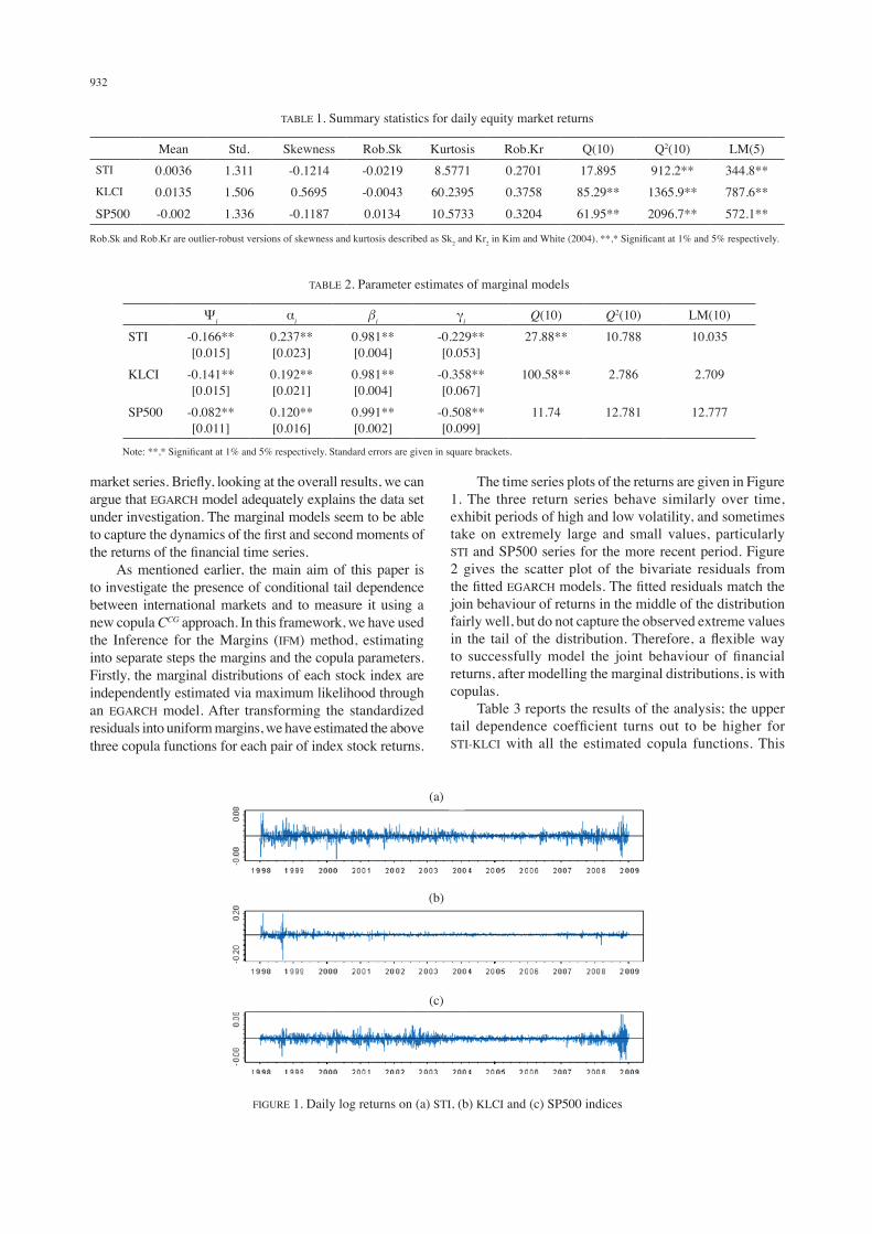
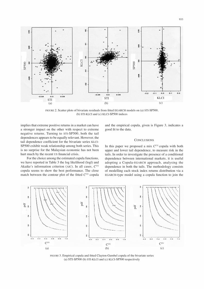
The time series plots of the returns are given in Figure 1. The three return series behave similarly over time, exhibit periods of high and low volatility, and sometimes take on extremely large and small values, particularly STI and SP500 series for the more recent period. Figure 2 gives the scatter plot of the bivariate residuals from the fitted EGARCH models. The fitted residuals match the join behaviour of returns in the middle of the distribution fairly well, but do not capture the observed extreme values in the tail of the distribution. Therefore, a flexible way to successfully model the joint behaviour of financial returns, after modelling the marginal distributions, is with copulas. Table 3 reports the results of the analysis; the upper tail dependence coefficient turns out to be higher for STI-KLCI with all the estimated copula functions. This

TABLE 2. Parameter estimates of marginal models

Ψi αi βi γi Q(10) Q2(10) LM(10)STI -0.166**

[0.015]0.237**[0.023]

0.981**[0.004]

-0.229**[0.053]

27.88** 10.788 10.035

KLCI -0.141**[0.015]

0.192**[0.021]

0.981**[0.004]

-0.358**[0.067]

100.58** 2.786 2.709

SP500 -0.082**[0.011]

0.120**[0.016]

0.991**[0.002]

-0.508**[0.099]

11.74 12.781 12.777

Note: **,* Significant at 1% and 5% respectively. Standard errors are given in square brackets.

TABLE 1. Summary statistics for daily equity market returns

Mean Std. Skewness Rob.Sk Kurtosis Rob.Kr Q(10) Q2(10) LM(5)STI 0.0036 1.311 -0.1214 -0.0219 8.5771 0.2701 17.895 912.2** 344.8**KLCI 0.0135 1.506 0.5695 -0.0043 60.2395 0.3758 85.29** 1365.9** 787.6**SP500 -0.002 1.336 -0.1187 0.0134 10.5733 0.3204 61.95** 2096.7** 572.1**

Rob.Sk and Rob.Kr are outlier-robust versions of skewness and kurtosis described as Sk2 and Kr2 in Kim and White (2004). **,* Significant at 1% and 5% respectively.

FIGURE 1. Daily log returns on (a) STI, (b) KLCI and (c) SP500 indices

(a)

(b)

(c)

933

implies that extreme positive returns in a market can have a stronger impact on the other with respect to extreme negative returns. Turning to STI-SP500, both the tail dependences appears to be equally relevant. However, the tail dependence coefficient for the bivariate series KLCI-SP500 exhibit weak relationship among both series. This is no surprise for the Malaysian economic has not been hurt much by the recent US financial crisis. For the choice among the estimated copula functions, we have reported in Table 3 the log likelihood (logl) and Akaike’s information criterion (AIC). In all cases, CCG copula seems to show the best performance. The close match between the contour plot of the fitted CCG copula

and the empirical copula, given is Figure 3, indicates a good fit to the data.

CONCLUSIONS

In this paper we proposed a mix CCG copula with both upper and lower tail dependence, to measure risk in the tails. In order to investigate the presence of a conditional dependence between international markets, it is useful adopting a Copula-EGARCH approach, analysing the dependence in both the tails. The methodology consists of modelling each stock index returns distribution via a EGARCH-type model using a copula function to join the

FIGURE 2. Scatter plots of bivariate residuals from fitted EGARCH models on (a) STI-SP500, (b) STI-KLCI and (c) KLCI-SP500 indices

KLCISTISTI

SP50

0

KLC

I

SP50

0

(a) (b) (c)

FIGURE 3. Empirical copula and fitted Clayton-Gumbel copula of the bivariate series (a) STI-SP500 (b) STI-KLCI and (c) KLCI-SP500 respectively

(a) (b) (c)CCGCCGCCG

pdf

pdf

pdf

934

TAB

LE 3

. Est

imat

es o

f the

par

amet

ers a

nd ta

il de

pend

ence

coe

ffici

ents

CC

CG

CJC

CC

G

θλ L

θλ U

θk

λ Uλ L

θζ

λ Uλ L

STI-

SP50

00.

1488

[0.0

23]

0.02

661.

0898

[0.0

13]

0.11

110.

1368

[0.0

34]

1.07

22[0

.027

10.

0912

0.00

631.

4282

[0.0

77]

1.42

82[0

.077

]0.

1326

0.01

76

STI-

KLC

I0.

7081

[0

.032

]0.

3757

1.36

54

[0.0

19]

0.33

860.

5288

[0

.041

]1.

3209

[0

.035

]0.

3099

0.26

961.

7946

[0.0

91]

1.79

46[0

.091

]0.

3496

0.35

19

KLC

I-SP

500

0.06

57[0

.025

]0.

0000

31.

0187

[0

.012

]0.

0252

0.06

57

[0.0

31]

1.00

00

[0.0

252]

0.00

000

0.00

003

1.03

41[0

.241

]1.

0341

[0.2

41]

0.00

004

0.00

01

Sta

ndar

d er

rors

are

giv

en in

squa

re b

rack

ets.

935

margins into a multivariate distribution. . In the empirical analysis we have used the CC, with lower tail dependence, the CJC and the CCG copulas with both upper and lower tail dependence. The result showed that CCG copula has a superior fit to our data compare to the other copulas used in this study.

REFERENCES

Abu Hassan, M.N., Shamiri, A. & Zaidi, I. 2009. Comparing the Accuracy of Density Forecasts from Competing GARCH Models. Sains Malaysiana 38(1): 95-104.

Abu Hassan, M.N. & Shamiri, A. 2007. Modeling and forecasting volatility of the Malaysian and the Singaporean stock indices using asymmetric GARCH models and non-normal densities. Malaysian Journal of Mathematical Sciences 1(1): 83-102.

Ang, A. & Bekaert, G. 2002. Short Rate Nonlinearities and Regime Switches. Journal of Economic Dynamics and Control 26(7-8): 1243-1274.

Ang, A. & Chen, J. 2002. Asymmetric Correlations of Equity Portfolios. Journal of Financial Economics 63(3): 443-494.

Bae, K.H., Karolyi, G.A. & Stulz, R.M. 2003. A New Approach to Measuring Financial Contagion. Review of Financial Studies 16(3): 217-263.

Cherubini, U., Luciano, E. & Vecchiato, W. 2004. Copula Methods in Finance. New York: John Wiley & Sons.

Embrechts, P., Kaufman, R. & Patie, P. 2005. Strategic longterm financial risks: Single risk factors. Computational Optimization Application 32(1-2): 61-90.

Embrechts, P., McNeil, A. & Straumann, D. 2002. Correlation and dependence in risk management: Properties and pitfalls. In Risk Management: Value at Risk and Beyond. M.A.H. Dempster (ed.): Cambridge: Cambridge University Press pp. 176-223.

Engle, R.F. 2002. Dynamic conditional correlation: a simple class of multivariate generalized autoregressive conditional heteroscedasticity models. Journal of Business and Economic Statistics 20: 339-350.

Gumbel, B. 1960. Atypischer Verlauf eines Schubkanals – Ein Kasuistischer Beitrag. Deutsche Zeitschrift furdie Gesamte Gerichtliche Medizin 50(2): 244-245.

Gumbel, E.J. 1960. Bivariate exponential distribution. Journal of the American Statistical Association 55: 698-707.

Hamo, Y., Masulis, R.W. & Ng, V. 1990. Correlations in price changes and volatility across international stock markets. The Review of Financial Studies 3: 281-307.

Hong, Y. 2001. A test for volatility spillover with application to exchange rates. Journal of Econometrics 103: 183-204.

Joe, H. & Xu, J. 1996. The estimation method of inference functions for margins for multivariate models. Technical Report No. 166, Department of Statistics, University of British Columbia, Vancouver.

Joe, H. 1997. Multivariate Models and Dependence Concepts. London: Chapman & Hall.

Jondeau, E. & Rockinger, M. 2006. The Copula-GARCH Model of Conditional Dependencies: an International Stock Market Application. Journal of International Money and Finance 25: 827-853.

Longin, F. & Solnik, B. 2001. Extreme Correlation of International Equity Markets. Journal of Finance 6(2): 649-676.

Miyakoshi T. 2003. Spillovers of stock return volatility to Asian equity markets from Japan and US. Journal of International Financial Markets, Institutions & Money 13: 383-399.

Nelson, D.B. 1991. Conditional heteroskedasticity in asset returns: a new approach. Econometrica 59(2): 347-370.

Nelsen, R.B. 2006. An Introduction to Copula. New york: Springer.

Sklar, A. 1959. Fonctions de répartition a n dimensions et leurs marges. Publications de ⎩’Institut de Statistique de L’Université de Paris 8: 229-231.

Institute of Mathematical Sciences Faculty of Science University of Malaya 50603 Kuala LumpurMalaysia

*Corresponding author; email: ahmed_shamir@um.edu.my

Received: 20 May 2010Accepted: 10 November 2010