Systematically Translating Service Level Objectives into Design and Operational Policies for Multi-Tier Applications Yuan Chen, Akhil Sahai, Subu Iyer, and Dejan Milojicic HP Laboratories Palo Alto HPL-2008-16 February 20, 2008* Service level management, SLA, performance model, muti-tier applications

We propose a systematic and practical approach that combines fine-grained performance modeling with regression analysis to translate Service Level Objectives (SLOs) into design and operational policies for multi-tier applications. These policies can then be used for designing a service to meet the SLOs and monitoring the service thereafter for violations at runtime. We demonstrate that our approach is practical and can be applied to commonly used multi-tier applications with different topologies and performance characteristics. Our approach handles both request-based and session-based workloads and deals with workload changes in terms of both request volume and transaction mix. Our approach is non-intrusive in the sense that it requires no specialized profiling, i.e., the data used in our approach is readily available from normal system and application monitoring. We validate our approach using both the RUBiS e-commerce benchmark and a trace-driven simulation of a business-critical enterprise application. These results show the effectiveness of our approach.

Internal Accession Date Only Approved for External Publication

© Copyright 2008 Hewlett-Packard Development Company, L.P.

Systematically Translating Service Level Objectives into

Design and Operational Policies for Multi-Tier Applications

Yuan Chen, Akhil Sahai, Subu Iyer, and Dejan Milojicic

Hewlett Packard Labs

ABSTRACT A Service Level Agreement (SLA) contains one or more Service

Level Objectives (SLOs) that describe the agreed upon quality

requirements at the service-level. In order to manage the service to

meet the agreed upon SLA, it is important not only to design a

service of the required capacity but also to monitor the service

thereafter for violations at runtime. This objective can be achieved

by undertaking SLA Decomposition, i.e., translating SLOs

specified in the SLA into lower-level policies that can then be

used for design and enforcement purposes. Such design and

operational policies are often constraints on thresholds of lower

level metrics. Traditionally, domain experts and administrators

bring their knowledge to bear upon the problem of SLA

decomposition. This practice is ad-hoc, manual, and static (i.e.,

done once). This is both costly, and not well suited to dynamic

workloads. In the past, there has been a number of efforts to

develop more automated and dynamic solutions, but these

approaches have many limitations and hence pose major

challenges to their applicability in practice.

In this paper, we propose a systematic and practical approach that

combines fine-grained performance modeling with regression

analysis to translate service level objectives directly into design

and operational policies for multi-tier applications. We

demonstrate that our approach is practical and can be applied to

commonly used multi-tier applications with different topologies

and performance characteristics. Our approach handles both

request-based and session-based workloads and deals with

workload changes in terms of both request volume and transaction

mix. Our approach is non-intrusive in the sense that it requires no

specialized profiling, i.e., the data used in our approach is readily

available from normal system and application monitoring. We

validate our approach using both the RUBis e-commerce

benchmark and a trace-driven simulation of a business-critical

enterprise application. These results show the effectiveness of our

approach.

1. INTRODUCTION A Service Level Agreement (SLA) captures the agreed upon

guarantees between a service provider and its customer. The

ability to deliver according to a pre-defined SLA is an

increasingly critical need in today’s highly complex and dynamic

IT environments.

One of the key tasks to SLA management is SLA decomposition,

translating the high level service objectives to low level design

and operational policies that can be then used to ensure the

Service Level Objectives (SLOs) are met. Given an

application/service and its corresponding SLOs, the IT operations

team undertakes SLA decomposition by determining the design

parameters that include identifying the operational level

objectives that are relevant and the healthy ranges for various

operational metrics to satisfy the SLAs. For example, for a given

set of SLOs for an e-commerce application (e.g., response time

requirements), domain experts make decisions about low level

design and operational policies. A design policy setting usually

contains system design parameters such as how many web servers,

application servers and database servers must be allocated to

satisfy the specified SLOs. An operational policy specifies details

of low level metrics (e.g., system resource utilization) to monitor,

healthy ranges of these metrics and actions to take when healthy

ranges are violated. Such an operational policy can be used for

monitoring potential violations and enforcement of SLOs at run

time. Once the system is put into production, workloads and

associated SLOs may change during operation. As a result, design

policies need to be adjusted to ensure current system capacity is

sufficient to handle the future workload. Operational policy

configurations need to be adjusted as well. Traditionally, domain

experts and administrators bring their knowledge to bear upon the

problem of SLA decomposition. Most of the time, these decisions

are made in an ad-hoc manner based on past experience. This

process involves substantial manual effort and adds to the cost of

service design and operation. Hence effective and efficient SLA

decomposition in an automated fashion is a key requirement in

SLA management.

In the past, researchers have made many efforts to address SLA

decomposition using techniques such as automated provisioning,

capacity planning, and monitoring [16, 17, 20, 28, 29]. Previous

studies have utilized performance models to guide resource

provisioning and capacity planning [16, 20]. Urgaonkar et al.

propose a dynamic provisioning technique for multi-tier

applications [16, 17]. All these research efforts separate design

and operations into two phases and mostly describe the capacity

planning and resource provisioning aspects of the design phase. In

addition, these research efforts make several simplifying

assumptions. As a result, the practicality and effectiveness of

these approaches pose major challenges to their applicability. We

have identified four main problems associated with existing

solutions that are described below.

First, workloads in real applications are dynamic and vary over

time. Unfortunately, most existing solutions take into account the

change in the volume of demand only, and assume a fixed or

stationary transaction mix [16, 17, 28]. Changes in the volume of

transactions (e.g., request rate) or the mixture of transaction types

can dramatically alter an application’s performance and resource.

Hence, a practical decomposition approach must handle workload

changes in both the volume and transaction mix.

Second, existing solutions model enterprise application workloads

as either request-based (open workload) or session-based (closed

workload) [16, 17, 26, 28]. In reality, workloads are typically

semi-open, which is significantly different than either an open or a

closed model [25]. Hence, a single model approach in most

existing solutions is not sufficient to handle the diversity in

realistic workloads. A practical approach should support multiple

models and choose an appropriate model that is based on the

properties of the real workload.

Third, building accurate performance models typically requires

input parameters such as resource demand. However, most

existing solutions cannot provide the needed model parameters

directly. Instead, such information must be obtained through

application or system instrumentation. In practice, instrumentation

of production applications is rarely done, as it is difficult, costly,

and may introduce overhead that degrades the application’s

performance [29]. Hence, a practical approach should be non-

intrusive and passively utilize data that is already available on

most systems.

Lastly, most existing solutions are not applicable to the diverse

range of design and implementation choices. Many of them make

simplifying assumptions about the application infrastructure, such

as considering only one server per tier [17, 26] or uniformly

distributing the requests across the different tiers [26]. To cope

with the diversity and complexity in real applications, a model

must be sufficiently general to capture the behavior of

applications with different configurations, workloads and

performance characteristics.

In this paper, we propose a systematic, non-intrusive and practical

SLA decomposition approach to address the above issues. Our

approach combines a fine-grain performance model and a

regression-based profiling approach to derive low-level

operational policies from high-level objectives for multi-tier

applications. We formalize the decomposition as a constraint

optimization problem, and develop a constraint solver to solve it.

Our approach provides the following four key contributions. First,

our approach formally characterizes both request-based and

session-based workloads. This enables us to choose an

appropriate model based on the workload characteristics of the

application. Second, our approach models workload as a

transaction mix, and systematically creates a resource profile for

each transaction type. This fine-grained model enables us to deal

with dynamic and non-stationary workloads. Third, we use

regression analysis to estimate the model parameters. The data

used in our approach is readily available from regular system and

application monitoring and requires no additional

instrumentation. It is hence practical to apply our approach to

production environments. Finally, the proposed modeling

technique can model multi-tier applications with different

topologies (i.e., any number of tiers and any number of servers at

each tier), and different workloads (open and/or closed). As a

result, our performance model and decomposition approach can

be applied to a vast variety of common multi-tier applications.

The remainder of this paper is organized as follows. Section 2

provides an overview of our approach and our workload model. In

Section 3, we describe profiling in detail. We present an analytical

performance model for multi-tier applications in Section 4 and

our decomposition approach in Section 5. The experimental

validation of our approach is presented in Section 6. Related

work is discussed in Section 7. Section 8 concludes the paper and

discusses future work.

2. OVERVIEW OF OUR APPROACH

2.1 Definition of a Multi-tier Application Multi-tier applications are common in modern enterprises. Such

applications are comprised of a large number of components,

which interact with one another in complex patterns. Typically,

multi-tier applications are structured into multiple logical tiers.

Each tier provides certain functionality to its preceding tier and

uses the functionality provided by its successor to carry out its

part of the overall request processing. At each tier, a load balancer

distributes the overall load among all servers of that tier according

to certain scheduling algorithms. Consider a multi-tier application

consisting of M tiers, T1, … TM. In the simplest case, each request

is processed exactly once by each tier and forwarded to its

succeeding tier for further processing. Once the result is processed

by the final tier TM, the results are sent back by each tier in the

reverse order until it reaches T1, which then sends the results to

the client. In more complex processing scenarios, each request at

tier Ti can trigger zero or multiple requests to tier Ti+1. For

example, a static web page request is processed by the Web tier

entirely and will not be forwarded to the other tiers. On the other

hand, a keyword search at a Web site may trigger multiple queries

to the database tier.

Table 1. Workload definition

2.2 Workload Model Definitions There are typically a number of transaction types in any multi-tier

application. For example, an online auction application has

transaction types such as login, browse, bid, etc. In most cases,

different transaction types have different service demands on

resources. For example, bid transactions in an auction site

typically require more CPU time than browse transactions. As

previously discussed, empirical workloads tend to be partially-

open, which means a user arrives and stays for a certain amount of

time (and issues a number of requests) before they leave. Previous

work has shown that partly-open workloads can be approximated

using an open workload if the number of requests in a session is

small, and a closed workload otherwise [25]. We consider these

two types of workloads in our workload model.

2.2.1 Open Workload In an open (request-based) workload, a new request to the

application is only triggered by a new user arrival. The requests

are independent of each other and the arrival rate is not influenced

by the number of requests that have already arrived and are being

processed. The number of users who interact with the application

at any time may range from zero to infinity. An open workload is

Type Workload Parameters

Open

N: number of transaction types

(λ1, λ2, … λN): transaction mix

where λ i (i =1 …N ) is the arrival rate of requests of

transaction type i during certain time interval

Closed

N: number of transaction types

C: number of users

Z: think time

π (p1, p2, … pi,…pN) : transaction mix distribution

where pi (i = 1, …N) is the percentage of requests of

transaction type i

characterized by an average arrival rate of requests or more

generally by an arrival distribution. A typical open workload is a

transaction mix of different transaction types. In real production

systems, the transaction mix changes over time [26]. Assume the

total number of transaction types is N. We define an open

workload during a certain interval (e.g., 5 minutes) as a vector (λ1,

λ2, … λN) where λi is the arrival rate of transaction type i during

that interval.

2.2.2 Closed Workload In a closed (session-based) workload, a fixed number of users

interact with the application and each of these users issues a

succession of requests. A new request from a user is only

triggered after the completion of a previous request by the same

user. A user submits a request, waits for the response of that

request, thinks for a certain time and then sends a new request.

The average time elapsed between the response from a previous

request and the submission of a new request by the same user is

called the “think time”, denoted by Z. The next request sent by a

user is usually determined by a state transition matrix that

specifies the probability to go from one transaction type to

another. Assume the number of transaction types is N. The state

transition matrix has N rows and N columns where pij represents

the transition probability from transaction type i to transaction

type j. Let P denote a state transition matrix of a closed workload

and π = (pi, p2…pN) denote the stationary transaction distribution

in a user session where pi presents the percentage of requests of

transaction type i sent by the user based on P. We have πP = π

and

1

1N

i

i

p=

=∑ . We can use the workload with a stationary

transaction mix π to approximate the behavior of a closed

workload with state transition matrix P [27]. A closed workload is

characterized by the number of concurrent users C, the stationary

distribution of transaction mix π, and the think time Z.

The open and closed workload models are summarized in Table 1.

Unlike many open workload models that assume a static

transaction mix and hence use an aggregate request rate to

characterize the workload, our transaction vector model captures

request rate per transaction type and hence can characterize

dynamic transaction mixes. Similarly, by explicitly incorporating

the transaction mix distribution as part of the workload parameter

in a closed workload, we can capture different behaviors with

different transaction distribution.

2.3 Our Approach An SLA is comprised of multiple Service Level Objectives

(SLOs). The task of SLA decomposition is to translate SLOs into

design parameters and bounds on low-level system resources such

that the high-level SLOs are met. Given a high-level performance

SLO and a workload for a multi-tier application (in terms of either

a transaction mix for an open workload or a transaction

distribution for a closed workload), decomposition provides the

resource requirements (e.g., number of servers) to handle the

workload and meet the specified SLO. It also finds the healthy

state of each component involved in providing the services (e.g.,

resource utilization). The decomposition process can be

summarized as

(R, W)� (ŋweb θweb-cpu, ŋapp, θapp-cpu,, ŋdb, θdb-cpu)

where R and W denote the response time and workload

respectively and ŋ is the number of servers at a tier and θ is the

resource utilization. SLA decomposition problem is the opposite

of a typical performance modeling problem, where the overall

system’s performance is predicted based on the configuration and

resource consumption of the sub-components.

For example, given the performance goal of a 3-tier online e-

commerce application (e.g., response time<10 seconds), and any

workload in term of transaction mix (e.g., browsing=10 reqs/s,

add-to-cart=5 reqs/s, and checkout=4 reqs/s), the decomposition

approach determines how many Web servers, application severs

and database severs are required to handle the workload while

satisfying the specified response time requirement. Decomposition

further determines the healthy ranges of the resource utilization of

each server (e.g., CPU, I/O, network, etc.) under the configuration

during operation.

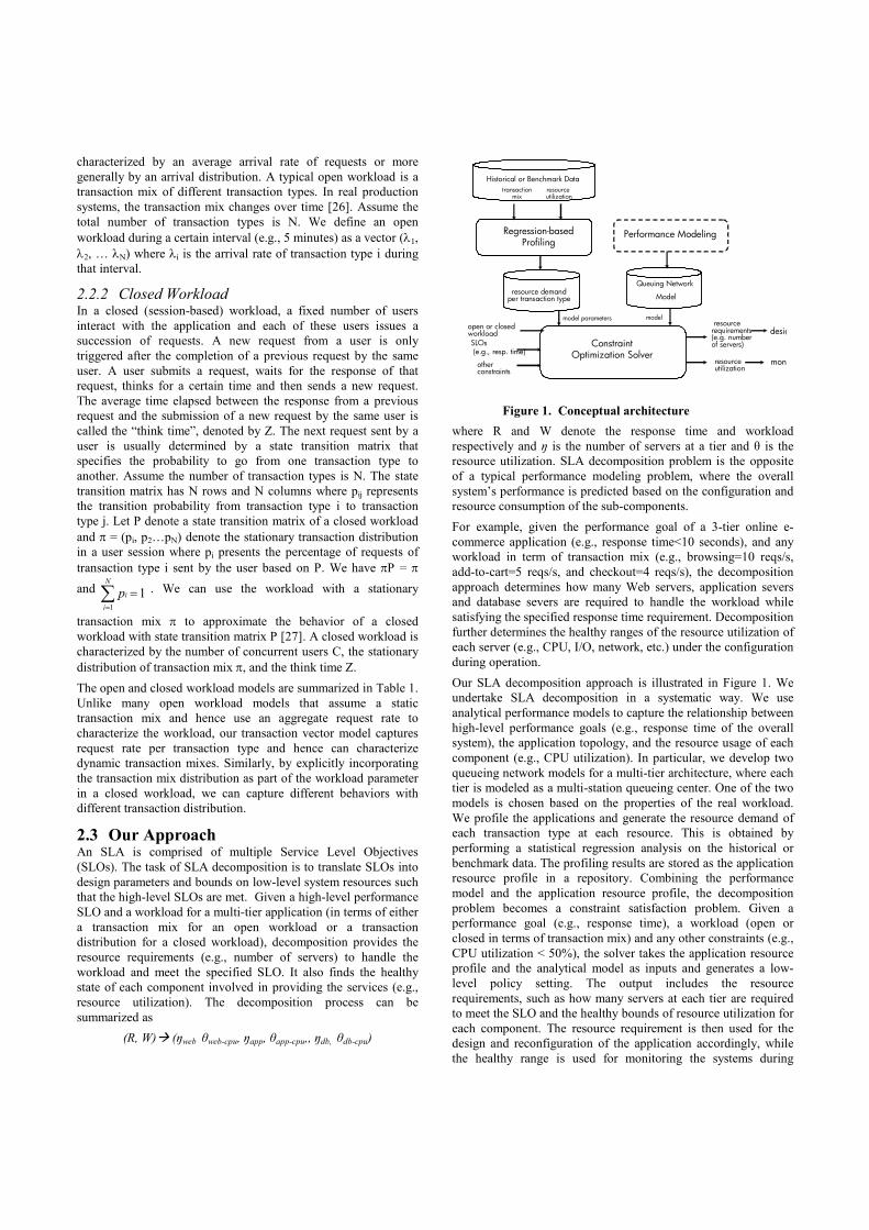
Our SLA decomposition approach is illustrated in Figure 1. We

undertake SLA decomposition in a systematic way. We use

analytical performance models to capture the relationship between

high-level performance goals (e.g., response time of the overall

system), the application topology, and the resource usage of each

component (e.g., CPU utilization). In particular, we develop two

queueing network models for a multi-tier architecture, where each

tier is modeled as a multi-station queueing center. One of the two

models is chosen based on the properties of the real workload.

We profile the applications and generate the resource demand of

each transaction type at each resource. This is obtained by

performing a statistical regression analysis on the historical or

benchmark data. The profiling results are stored as the application

resource profile in a repository. Combining the performance

model and the application resource profile, the decomposition

problem becomes a constraint satisfaction problem. Given a

performance goal (e.g., response time), a workload (open or

closed in terms of transaction mix) and any other constraints (e.g.,

CPU utilization < 50%), the solver takes the application resource

profile and the analytical model as inputs and generates a low-

level policy setting. The output includes the resource

requirements, such as how many servers at each tier are required

to meet the SLO and the healthy bounds of resource utilization for

each component. The resource requirement is then used for the

design and reconfiguration of the application accordingly, while

the healthy range is used for monitoring the systems during

Figure 1. Conceptual architecture

Regression-based Profiling

transactionmix

resource utilization

resource demand per transaction type

Historical or Benchmark Data

Performance Modeling

Queuing Network

Model

Constraint Optimization Solver

model parameters model

open or closed workload SLOs(e.g., resp. time)

resource requirements (e.g. number of servers)

resource utilizationother

constraints

design

monitoring

operation. The developed analytical models and application

resource profiles are archived for future reuse. If the workload or

response times change, we only need to re-solve the constraint

satisfaction problem with new parameters to generate a new

policy setting.

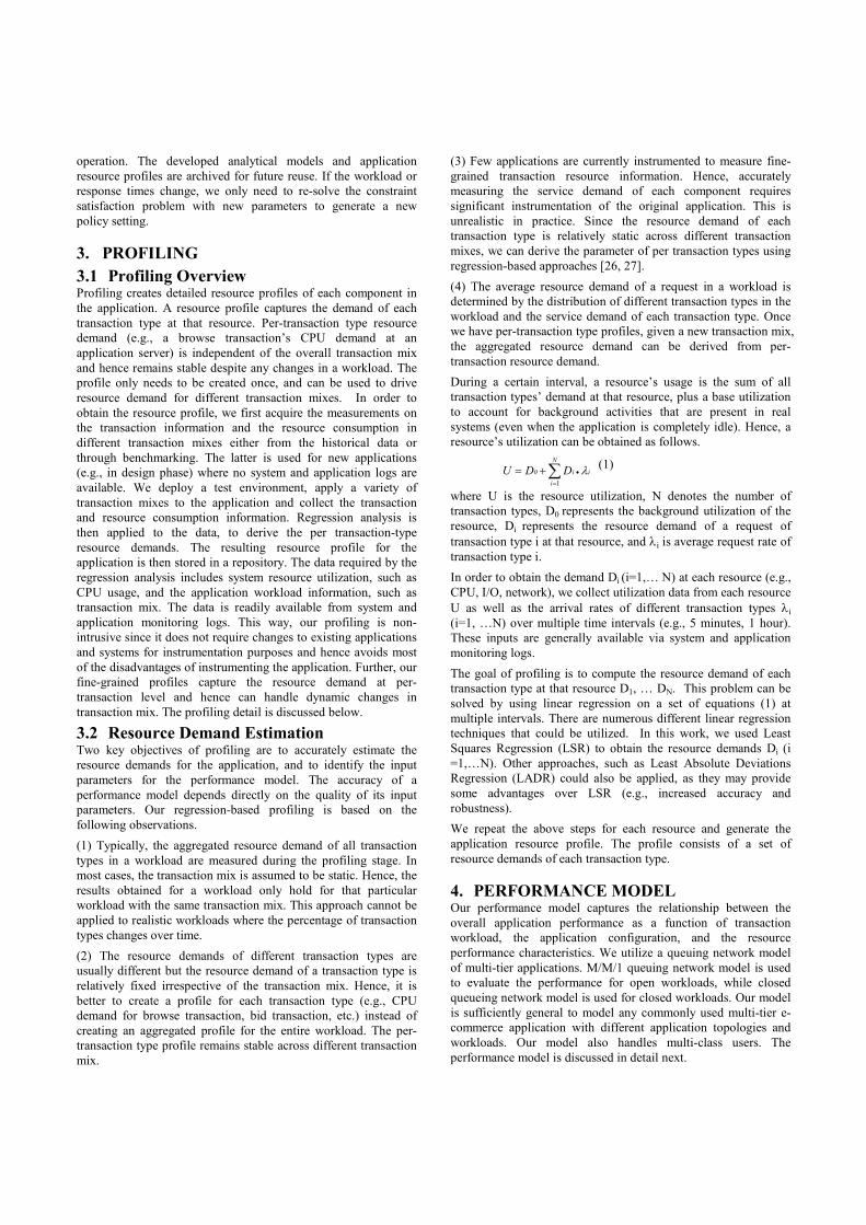
3. PROFILING

3.1 Profiling Overview Profiling creates detailed resource profiles of each component in

the application. A resource profile captures the demand of each

transaction type at that resource. Per-transaction type resource

demand (e.g., a browse transaction’s CPU demand at an

application server) is independent of the overall transaction mix

and hence remains stable despite any changes in a workload. The

profile only needs to be created once, and can be used to drive

resource demand for different transaction mixes. In order to

obtain the resource profile, we first acquire the measurements on

the transaction information and the resource consumption in

different transaction mixes either from the historical data or

through benchmarking. The latter is used for new applications

(e.g., in design phase) where no system and application logs are

available. We deploy a test environment, apply a variety of

transaction mixes to the application and collect the transaction

and resource consumption information. Regression analysis is

then applied to the data, to derive the per transaction-type

resource demands. The resulting resource profile for the

application is then stored in a repository. The data required by the

regression analysis includes system resource utilization, such as

CPU usage, and the application workload information, such as

transaction mix. The data is readily available from system and

application monitoring logs. This way, our profiling is non-

intrusive since it does not require changes to existing applications

and systems for instrumentation purposes and hence avoids most

of the disadvantages of instrumenting the application. Further, our

fine-grained profiles capture the resource demand at per-

transaction level and hence can handle dynamic changes in

transaction mix. The profiling detail is discussed below.

3.2 Resource Demand Estimation Two key objectives of profiling are to accurately estimate the

resource demands for the application, and to identify the input

parameters for the performance model. The accuracy of a

performance model depends directly on the quality of its input

parameters. Our regression-based profiling is based on the

following observations.

(1) Typically, the aggregated resource demand of all transaction

types in a workload are measured during the profiling stage. In

most cases, the transaction mix is assumed to be static. Hence, the

results obtained for a workload only hold for that particular

workload with the same transaction mix. This approach cannot be

applied to realistic workloads where the percentage of transaction

types changes over time.

(2) The resource demands of different transaction types are

usually different but the resource demand of a transaction type is

relatively fixed irrespective of the transaction mix. Hence, it is

better to create a profile for each transaction type (e.g., CPU

demand for browse transaction, bid transaction, etc.) instead of

creating an aggregated profile for the entire workload. The per-

transaction type profile remains stable across different transaction

mix.

(3) Few applications are currently instrumented to measure fine-

grained transaction resource information. Hence, accurately

measuring the service demand of each component requires

significant instrumentation of the original application. This is

unrealistic in practice. Since the resource demand of each

transaction type is relatively static across different transaction

mixes, we can derive the parameter of per transaction types using

regression-based approaches [26, 27].

(4) The average resource demand of a request in a workload is

determined by the distribution of different transaction types in the

workload and the service demand of each transaction type. Once

we have per-transaction type profiles, given a new transaction mix,

the aggregated resource demand can be derived from per-

transaction resource demand.

During a certain interval, a resource’s usage is the sum of all

transaction types’ demand at that resource, plus a base utilization

to account for background activities that are present in real

systems (even when the application is completely idle). Hence, a

resource’s utilization can be obtained as follows.

1

N

0 i i

i

U D D λ•=

= +∑ (1)

where U is the resource utilization, N denotes the number of

transaction types, D0 represents the background utilization of the

resource, Di represents the resource demand of a request of

transaction type i at that resource, and λi is average request rate of

transaction type i.

In order to obtain the demand Di (i=1,… N) at each resource (e.g.,

CPU, I/O, network), we collect utilization data from each resource

U as well as the arrival rates of different transaction types λi

(i=1, …N) over multiple time intervals (e.g., 5 minutes, 1 hour).

These inputs are generally available via system and application

monitoring logs.

The goal of profiling is to compute the resource demand of each

transaction type at that resource D1, … DN. This problem can be

solved by using linear regression on a set of equations (1) at

multiple intervals. There are numerous different linear regression

techniques that could be utilized. In this work, we used Least

Squares Regression (LSR) to obtain the resource demands Di (i

=1,…N). Other approaches, such as Least Absolute Deviations

Regression (LADR) could also be applied, as they may provide

some advantages over LSR (e.g., increased accuracy and

robustness).

We repeat the above steps for each resource and generate the

application resource profile. The profile consists of a set of

resource demands of each transaction type.

4. PERFORMANCE MODEL Our performance model captures the relationship between the

overall application performance as a function of transaction

workload, the application configuration, and the resource

performance characteristics. We utilize a queuing network model

of multi-tier applications. M/M/1 queuing network model is used

to evaluate the performance for open workloads, while closed

queueing network model is used for closed workloads. Our model

is sufficiently general to model any commonly used multi-tier e-

commerce application with different application topologies and

workloads. Our model also handles multi-class users. The

performance model is discussed in detail next.

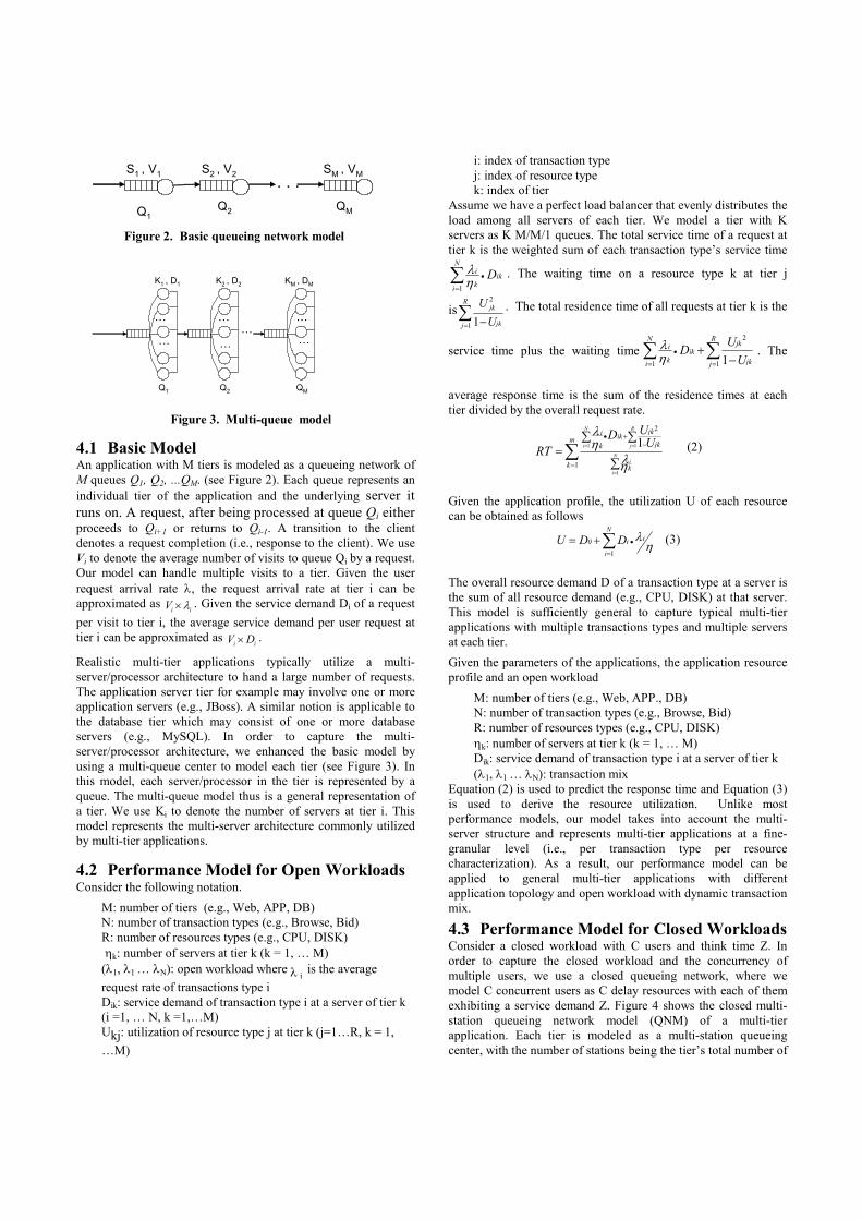
4.1 Basic Model An application with M tiers is modeled as a queueing network of

M queues Q1, Q2, ...QM. (see Figure 2). Each queue represents an

individual tier of the application and the underlying server it

runs on. A request, after being processed at queue Qi either proceeds to Qi+1 or returns to Qi-1. A transition to the client

denotes a request completion (i.e., response to the client). We use

Vi to denote the average number of visits to queue Qi by a request.

Our model can handle multiple visits to a tier. Given the user

request arrival rate λ, the request arrival rate at tier i can be

approximated as i iV λ× . Given the service demand Di of a request

per visit to tier i, the average service demand per user request at

tier i can be approximated as i iV D× .

Realistic multi-tier applications typically utilize a multi-

server/processor architecture to hand a large number of requests.

The application server tier for example may involve one or more

application servers (e.g., JBoss). A similar notion is applicable to

the database tier which may consist of one or more database

servers (e.g., MySQL). In order to capture the multi-

server/processor architecture, we enhanced the basic model by

using a multi-queue center to model each tier (see Figure 3). In

this model, each server/processor in the tier is represented by a

queue. The multi-queue model thus is a general representation of

a tier. We use Ki to denote the number of servers at tier i. This

model represents the multi-server architecture commonly utilized

by multi-tier applications.

4.2 Performance Model for Open Workloads Consider the following notation.

M: number of tiers (e.g., Web, APP, DB)

N: number of transaction types (e.g., Browse, Bid)

R: number of resources types (e.g., CPU, DISK)

ηk: number of servers at tier k (k = 1, … M)

(λ1, λ1 … λN): open workload where λ i is the average

request rate of transactions type i Dik: service demand of transaction type i at a server of tier k

(i =1, … N, k =1,…M) Ukj: utilization of resource type j at tier k (j=1…R, k = 1,

…M)

i: index of transaction type

j: index of resource type

k: index of tier

Assume we have a perfect load balancer that evenly distributes the

load among all servers of each tier. We model a tier with K

servers as K M/M/1 queues. The total service time of a request at

tier k is the weighted sum of each transaction type’s service time

1

Ni

ikk

i

Dλη

•

=∑ . The waiting time on a resource type k at tier j

is2

1 1

Rjk

jkj

U

U= −∑ . The total residence time of all requests at tier k is the

service time plus the waiting time

2

1 1 1

N Rjki

ikk jki j

UD

U

λη

•

= =

+−∑ ∑ . The

average response time is the sum of the residence times at each

tier divided by the overall request rate.

1 1

1

2

1

1

N R

i j

Ni

i

jkiikm

jkk

k k

UDU

RT

λη

λη

= =

=

• +−

=

∑ ∑=

∑∑ (2)

Given the application profile, the utilization U of each resource

can be obtained as follows

1

N

i0 i

i

U D D λη•

=

= +∑ (3)

The overall resource demand D of a transaction type at a server is

the sum of all resource demand (e.g., CPU, DISK) at that server.

This model is sufficiently general to capture typical multi-tier

applications with multiple transactions types and multiple servers

at each tier.

Given the parameters of the applications, the application resource

profile and an open workload

M: number of tiers (e.g., Web, APP., DB)

N: number of transaction types (e.g., Browse, Bid)

R: number of resources types (e.g., CPU, DISK)

ηk: number of servers at tier k (k = 1, … M)

Dik: service demand of transaction type i at a server of tier k

(λ1, λ1 … λN): transaction mix Equation (2) is used to predict the response time and Equation (3)

is used to derive the resource utilization. Unlike most

performance models, our model takes into account the multi-

server structure and represents multi-tier applications at a fine-

granular level (i.e., per transaction type per resource

characterization). As a result, our performance model can be

applied to general multi-tier applications with different

application topology and open workload with dynamic transaction

mix.

4.3 Performance Model for Closed Workloads Consider a closed workload with C users and think time Z. In

order to capture the closed workload and the concurrency of

multiple users, we use a closed queueing network, where we

model C concurrent users as C delay resources with each of them

exhibiting a service demand Z. Figure 4 shows the closed multi-

station queueing network model (QNM) of a multi-tier

application. Each tier is modeled as a multi-station queueing

center, with the number of stations being the tier’s total number of

Q1

S1 , V1

Q2 QM

S2 , V2 SM , VM

. . .

Figure 2. Basic queueing network model

Figure 3. Multi-queue model

Q1

K1 , D1

…

…

… …

…

Q2 QM

K2 , D2 KM , DM

……

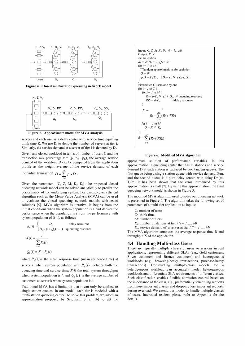
servers and each user is a delay center with service time equaling

think time Z. We use Ki to denote the number of servers at tier i.

Similarly, the service demand at a server of tier i is denoted by Di.

Given any closed workload in terms of number of users C and the

transaction mix percentage π = (pi, p2…pK), the average service

demand of the workload D can be computed from the application

profile as the weight average of the service demand of each

individual transaction

1

N

i i

i

D p D•=

=∑ .

Given the parameters {C, Z, M, Ki, Di}, the proposed closed

queueing network model can be solved analytically to predict the

performance of the underlying system. For example, an efficient

algorithm such as the Mean-Value Analysis (MVA) can be used

to evaluate the closed queueing network models with exact

solutions [5]. MVA algorithm is iterative. It begins from the

initial conditions when the system population is 1 and derives the

performance when the population is i from the performance with

system population of (i-1), as follows

delay resource( )

(1 ( 1) queueing resource

k

k

k k

DR i

D Q i

=

× + −

1

( )

( )K

k

k

iX i

R i=

=

∑

( ) ( )k kQ i X R i= ×

where ( )kR i is the mean response time (mean residence time) at

server k when system population is i; ( )kR i includes both the

queueing time and service time; X(i) the total system throughput

when system population is i; and ( )kQ i is the average number of

customers at server k when system population is i.

Traditional MVA has a limitation that it can only be applied to

single-station queues. In our model, each tier is modeled with a

multi-station queueing center. To solve this problem, we adopt an

approximation proposed by Seidmann et al. [6] to get the

approximate solution of performance variables. In this

approximation, a queueing center that has m stations and service

demand D at each station is replaced by two tandem queues. The

first queue being a single-station queue with service demand D/m,

and the second queue is a pure delay center, with delay D×(m-

1)/m. It has been shown that the error introduced by this

approximation is small [7]. By using this approximation, the final

queueing network model is shown in Figure 5.

The modified MVA algorithm used to solve our queueing network

is presented in Figure 6. The algorithm takes the following set of

parameters of a multi-tier application as inputs:

C: number of users

Z: think time

M: number of tiers

Ki: number of stations at tier i (i = 1,…, M)

Di: service demand of a server at tier i (i = 1,…, M)

The MVA algorithm computes the average response time R and

throughput X of the application.

4.4 Handling Multi-class Users There are typically multiple classes of users or sessions in real

applications, representing different SLAs (e.g., Gold customers,

Sliver customers and Bronze customers) and heterogeneous

workloads (e.g., browsing-heavy transactions, purchase-heavy

transactions). Constructing multiple-class models for a

heterogeneous workload can accurately model heterogeneous

workloads and differentiate SLA requirements of different classes.

Such classification enables flexible admission control based on

the importance of the class, e.g., preferentially scheduling requests

from more important classes and dropping less important requests

during overload. We extend our model to handle multiple classes

of users. Interested readers, please refer to Appendix for the

details.

Input: C, Z, M, Ki, Di, (i = 1,.. M)

Output: R, X

//initialization

R0 = Z; D0 = Z; Q0 = 0;

for i = 1 to M {

// Tandem approximations for each tier

Qi = 0;

qrDi = Di/Ki ; drDi = Di × ( Ki-1)/Ki ;

}

//introduce C users one by one

for i = 1 to C {

for j = 1 to M {

Rj = qrDj × (1 + Qj); // queueing resource

RRj = drDj; //delay resource

}

)(1

0 ∑=

++=

m

j

ii RRRR

iX

for j = 1 to M

Qj = X × Rj;

}

R = )(1

∑=

+M

i

ii RRR

Figure 6. Modified MVA algorithm

Figure 4. Closed multi-station queueing network model

…

…

Users

C , Z, V0

Q1

K1 , S1 , V1

…

…

… …

…

Q2 QM

K2 , S2 , V2 KM , SM , VM

……

Figure 5. Approximate model for MVA analysis

Users

N , Z, V0

Q1

V1, D1, DD1

Q2QM

……

…

V2, D2, DD2 VM, DM, DDM

5. DECOMPOSITION Given an SLO (e.g., response time) and a workload, the goal of

decomposition is to determine the design parameters (e.g., number

of servers at each tier) to guarantee that the system has enough

capacity for processing the specified workload and meeting the

proposed SLO. The output of decomposition contains operational

policy settings such as

• how many servers are required for each tier

• what’s the CPU, Memory, IO utilization of each server

As we discussed before, we generate the profile based on the

historical data or benchmarking data with varying workloads. The

service demand of each individual transaction type is retrieved

from the archive, as shown in Figure 1. Given any workload and a

response time requirement, the task of decomposition is then to

find the set of model input parameters such as number of servers

that satisfy the response time requirement and further derive the

resource utilization. Decomposition thus becomes a constraint

satisfaction problem. We have developed a simple constraint

satisfaction solver to solve this problem. The solver takes

performance goal, workload, resource profiles and performance

model as inputs and constructs a set of constraint equations.

Various constraint satisfaction algorithms, such as linear

programming and optimization techniques, are available to solve

such problems [21]. Typically, the solution is non-deterministic

and the solution space is large. However, for the problems we are

studying, the search space is relatively small. For example, if we

consider assigning the number of servers at each tier, we can

efficiently enumerate the entire solution space to find a solution.

Also, we are often interested in finding a single feasible solution

(rather than the optimal solution), so we can stop the search once

one is found. Other heuristic techniques can also be used during

the search. For example, the hint that the response time typically

decreases with respect to the increase of allocated resources can

also reduce the search space.

One advantage of our approach is that once the profile and model

are created, they can be repeatedly used to perform decomposition

for different SLOs and workloads. That is, if the response time or

workload changes, we only need to resolve the constraint

satisfaction problem with the new parameters. Similarly, if the

application is deployed to a new environment, we only need to

regenerate the profile in that environment using regression

analysis. Further, given high-level goals and resource availability,

we can apply our decomposition approach for automatic selection

of resources and for the generation of sizing specifications that

could be used during system deployment.

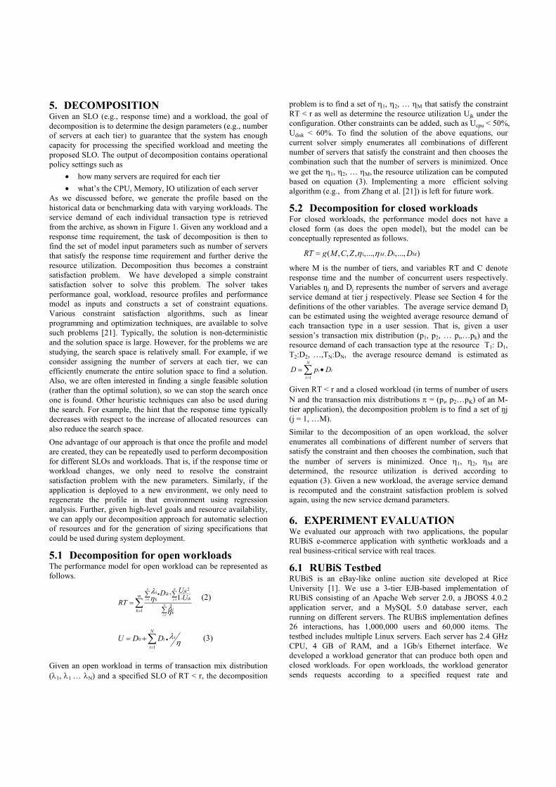
5.1 Decomposition for open workloads The performance model for open workload can be represented as

follows.

1 1

1

2

1

1

N R

i j

Ni

i

jkiikm

jkk

k k

UDU

RT

λη

λη

= =

=

• +−

=

∑ ∑=

∑∑

(2)

1

N

i0 i

i

U D D λη•

=

= +∑ (3)

Given an open workload in terms of transaction mix distribution

(λ1, λ1 … λN) and a specified SLO of RT < r, the decomposition

problem is to find a set of η1, η2, … ηM that satisfy the constraint

RT < r as well as determine the resource utilization Ujk under the

configuration. Other constraints can be added, such as Ucpu < 50%,

Udisk < 60%. To find the solution of the above equations, our

current solver simply enumerates all combinations of different

number of servers that satisfy the constraint and then chooses the

combination such that the number of servers is minimized. Once

we get the η1, η2, … ηM, the resource utilization can be computed

based on equation (3). Implementing a more efficient solving

algorithm (e.g., from Zhang et al. [21]) is left for future work.

5.2 Decomposition for closed workloads For closed workloads, the performance model does not have a

closed form (as does the open model), but the model can be

conceptually represented as follows.

1 , 1( , , , ,..., ,..., )M MRT g M C Z D Dη η=

where M is the number of tiers, and variables RT and C denote

response time and the number of concurrent users respectively.

Variables ŋj and Dj represents the number of servers and average

service demand at tier j respectively. Please see Section 4 for the

definitions of the other variables. The average service demand Dj

can be estimated using the weighted average resource demand of

each transaction type in a user session. That is, given a user

session’s transaction mix distribution (p1, p2, … pi,…pk) and the

resource demand of each transaction type at the resource T1: D1,

T2:D2, …,TN:DN, the average resource demand is estimated as

1

N

i i

i

D p D=

= •∑

Given RT < r and a closed workload (in terms of number of users

N and the transaction mix distributions π = (pi, p2…pK) of an M-

tier application), the decomposition problem is to find a set of ŋj

(j = 1, …M).

Similar to the decomposition of an open workload, the solver

enumerates all combinations of different number of servers that

satisfy the constraint and then chooses the combination, such that

the number of servers is minimized. Once η1, η2, ηM are

determined, the resource utilization is derived according to

equation (3). Given a new workload, the average service demand

is recomputed and the constraint satisfaction problem is solved

again, using the new service demand parameters.

6. EXPERIMENT EVALUATION We evaluated our approach with two applications, the popular

RUBiS e-commerce application with synthetic workloads and a

real business-critical service with real traces.

6.1 RUBiS Testbed RUBiS is an eBay-like online auction site developed at Rice

University [1]. We use a 3-tier EJB-based implementation of

RUBiS consisting of an Apache Web server 2.0, a JBOSS 4.0.2

application server, and a MySQL 5.0 database server, each

running on different servers. The RUBiS implementation defines

26 interactions, has 1,000,000 users and 60,000 items. The

testbed includes multiple Linux servers. Each server has 2.4 GHz

CPU, 4 GB of RAM, and a 1Gb/s Ethernet interface. We

developed a workload generator that can produce both open and

closed workloads. For open workloads, the workload generator

sends requests according to a specified request rate and

transaction mix. For closed workloads, the workload follows a

given transition matrix to simulate multiple concurrent users

interactions with RUBiS. The workload generator runs on a

separate server node from any of the RUBiS systems.

6.1.1 Performance Prediction To validate the correctness and accuracy of our model, we

compare the response times predicted by our model and actual

measurements with different workloads under different

configurations.

We use the workload generator to produce variable workloads

with fluctuations in request rate and transaction mix. Application

data is obtained from Apache and JBoss log. System utilization is

collected every one minute using the SAR monitor. The data set

records two kinds of data about RUBiS, application-level data

such as transaction request rate of each transaction type, and

system level resource utilization (e.g., CPU utilization). We then

apply the regression analysis described in Section 3 to generate

the application’s resource profile. Given any open or closed

workload, we use the resource demand information obtained

during profiling as model input parameters, and apply the

performance model described in section 4 to derive the response

time.

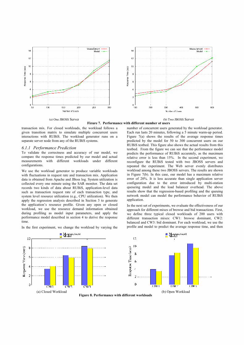
In the first experiment, we change the workload by varying the

number of concurrent users generated by the workload generator.

Each run lasts 20 minutes, following a 5 minute warm-up period.

Figure 7(a) shows the results of the average response times

predicted by the model for 50 to 300 concurrent users on our

RUBiS testbed. This figure also shows the actual results from this

testbed. From the figure we can see that the performance model

predicts the performance of RUBiS accurately, as the maximum

relative error is less than 15%. In the second experiment, we

reconfigure the RUBiS tested with two JBOSS servers and

repeated the experiment. The Web server evenly distributes

workload among these two JBOSS servers. The results are shown

in Figure 7(b). In this case, our model has a maximum relative

error of 20%. It is less accurate than single application server

configuration due to the error introduced by multi-station

queueing model and the load balancer overhead. The above

results show that the regression-based profiling and the queuing

network model can model the performance behavior of RUBiS

application.

In the next set of experiments, we evaluate the effectiveness of our

approach for different mixes of browse and bid transactions. First,

we define three typical closed workloads of 200 users with

different transaction mixes: CW1: browse dominant, CW2:

balanced and CW3: bid dominant. For each workload, we use the

profile and model to predict the average response time, and then

Figure 8. Performance with different workloads (a) Closed Workload (b) Open Workload

Figure 7. Performance with different number of users

(a) One JBOSS Server (b) Two JBOSS Server

compare the results with the actual performance. The results are

depicted in Figure 8(a). The results show that our model can

accurately predict the performance for different closed workloads

with different transaction mixes. Similarly, we define three typical

open workloads with different transaction mixes: OW1, OW2 and

OW3 and compare the accuracy of response time predicted by our

model for each workloads. The results depicted in Figure 8(b)

indicate that our model can also work well with open workloads.

These results clearly demonstrate that our model can use the same

profiling results (i.e., model input parameters) obtained during

profiling to predict the performance of any unforeseen transaction

mixes.

We also conducted a similar evaluation of the RUBiS

configuration with 2 JBOSS servers. We obtained similar results,

and thus do not include the figures here.

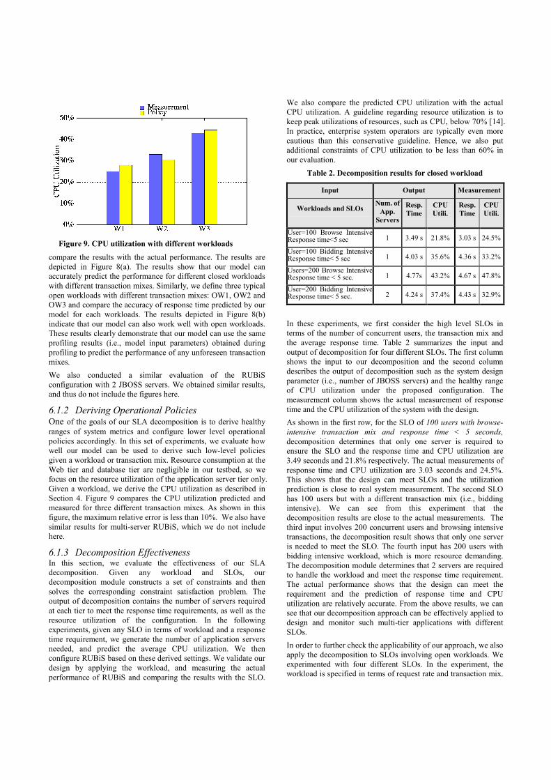
6.1.2 Deriving Operational Policies One of the goals of our SLA decomposition is to derive healthy

ranges of system metrics and configure lower level operational

policies accordingly. In this set of experiments, we evaluate how

well our model can be used to derive such low-level policies

given a workload or transaction mix. Resource consumption at the

Web tier and database tier are negligible in our testbed, so we

focus on the resource utilization of the application server tier only.

Given a workload, we derive the CPU utilization as described in

Section 4. Figure 9 compares the CPU utilization predicted and

measured for three different transaction mixes. As shown in this

figure, the maximum relative error is less than 10%. We also have

similar results for multi-server RUBiS, which we do not include

here.

6.1.3 Decomposition Effectiveness In this section, we evaluate the effectiveness of our SLA

decomposition. Given any workload and SLOs, our

decomposition module constructs a set of constraints and then

solves the corresponding constraint satisfaction problem. The

output of decomposition contains the number of servers required

at each tier to meet the response time requirements, as well as the

resource utilization of the configuration. In the following

experiments, given any SLO in terms of workload and a response

time requirement, we generate the number of application servers

needed, and predict the average CPU utilization. We then

configure RUBiS based on these derived settings. We validate our

design by applying the workload, and measuring the actual

performance of RUBiS and comparing the results with the SLO.

We also compare the predicted CPU utilization with the actual

CPU utilization. A guideline regarding resource utilization is to

keep peak utilizations of resources, such as CPU, below 70% [14].

In practice, enterprise system operators are typically even more

cautious than this conservative guideline. Hence, we also put

additional constraints of CPU utilization to be less than 60% in

our evaluation.

Table 2. Decomposition results for closed workload

In these experiments, we first consider the high level SLOs in

terms of the number of concurrent users, the transaction mix and

the average response time. Table 2 summarizes the input and

output of decomposition for four different SLOs. The first column

shows the input to our decomposition and the second column

describes the output of decomposition such as the system design

parameter (i.e., number of JBOSS servers) and the healthy range

of CPU utilization under the proposed configuration. The

measurement column shows the actual measurement of response

time and the CPU utilization of the system with the design.

As shown in the first row, for the SLO of 100 users with browse-

intensive transaction mix and response time < 5 seconds,

decomposition determines that only one server is required to

ensure the SLO and the response time and CPU utilization are

3.49 seconds and 21.8% respectively. The actual measurements of

response time and CPU utilization are 3.03 seconds and 24.5%.

This shows that the design can meet SLOs and the utilization

prediction is close to real system measurement. The second SLO

has 100 users but with a different transaction mix (i.e., bidding

intensive). We can see from this experiment that the

decomposition results are close to the actual measurements. The

third input involves 200 concurrent users and browsing intensive

transactions, the decomposition result shows that only one server

is needed to meet the SLO. The fourth input has 200 users with

bidding intensive workload, which is more resource demanding.

The decomposition module determines that 2 servers are required

to handle the workload and meet the response time requirement.

The actual performance shows that the design can meet the

requirement and the prediction of response time and CPU

utilization are relatively accurate. From the above results, we can

see that our decomposition approach can be effectively applied to

design and monitor such multi-tier applications with different

SLOs.

In order to further check the applicability of our approach, we also

apply the decomposition to SLOs involving open workloads. We

experimented with four different SLOs. In the experiment, the

workload is specified in terms of request rate and transaction mix.

Input Output Measurement

Workloads and SLOs Num. of

App.

Servers

Resp.

Time

CPU

Utili.

Resp.

Time

CPU

Utili.

User=100 Browse IntensiveResponse time<5 sec 1 3.49 s 21.8% 3.03 s 24.5%

User=100 Bidding IntensiveResponse time< 5 sec 1 4.03 s 35.6% 4.36 s 33.2%

Users=200 Browse Intensive Response time < 5 sec. 1 4.77s 43.2% 4.67 s 47.8%

User=200 Bidding Intensive Response time< 5 sec. 2 4.24 s 37.4% 4.43 s 32.9%

Figure 9. CPU utilization with different workloads

These results are summarized in Table 3. The results show that

our approach can also work well with open workloads.

Table 3. Decomposition results for open workload

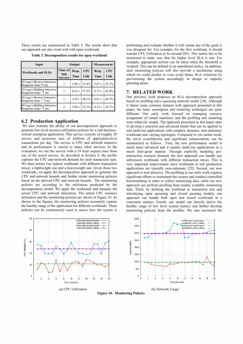
6.2 Production Application We also evaluate the ability of our decomposition approach to

generate low-level resource utilization policies for a real business-

critical enterprise application. This service consists of roughly 20

servers and processes tens of millions of application-level

transactions per day. The service is CPU and network intensive

and its performance is crucial to many other services. In the

evaluation, we run the service with a 24 hour request trace from

one of the actual servers. As described in Section 3, the profile

captures the CPU and network demand for each transaction type.

We then extract two typical workloads with different transaction

mixes: a lightweight one and a heavyweight one. Given these two

workloads, we apply the decomposition approach to generate the

CPU and network bounds and further create monitoring policies

based on the derived CPU and network bounds. The monitoring

policies are according to the utilization predicted by the

decomposition model. We apply the workloads and measure the

actual CPU and network utilization. The actual CPU resource

utilization and the monitoring policies are shown in Figure 10. As

shown in the figures, the monitoring policies accurately capture

the healthy range of the application for different workloads. These

policies can be continuously used to assess how the system is

performing and evaluate whether it will violate any of the goals it

was designed for. For example, for the first workload, it should

warrant CPU Utilization to be around 20%. This metric has to be

monitored to make sure that the higher level SLA is met. For

example, appropriate actions can be taken when the threshold is

violated. This can be defined in an operational policy. In addition,

such monitoring policies will also provide a mechanism using

which we could predict or even avoid future SLA violations by

provisioning the system accordingly in design or capacity

planning phase.

7. RELATED WORK Our previous work proposes an SLA decomposition approach

based on profiling and a queueing network model [28]. Although

it shares some common features with approach presented in this

paper, the basic assumption and modeling techniques are quite

different. Our early work focused on managing resource

assignment of virtual machines, and the profiling and modeling

were relatively simple. The approach presented in this paper aims

to develop a practical and advanced model that can be applied to

real multi-tier applications with complex, dynamic, non-stationary

workloads and varying topologies. Compared to our earlier work,

the novel contributions and significant enhancements can be

summarized as follows. First, the new performance model is

much more advanced and it models multi-tier applications in a

much finer-grain manner. Through explicitly modeling per-

transaction resource demand, the new approach can handle any

unforeseen workloads with different transaction mixes. This is

very important improvement since workloads in real production

applications are typically non-stationary [25]. Second, our new

approach is non-intrusive. The profiling in our early work requires

significant efforts to instrument the system and conduct controlled

benchmarking in order to collect monitoring data, while our new

approach can perform profiling from readily available monitoring

data. Third, by defining the workload as transaction mix and

introducing open queueing and closed queuing models, our

approach can handle both open and closed workloads in a

consistent manner. Fourth, our model can directly derive the

healthy range of low level system metrics and further develop

monitoring policies from the profiles. We also increased the

Input Output Measurement

Workloads and SLOs Num. of

App.

Servers

Resp.

Time

CPU

Utili.

Resp.

Time

CPU

Utili.

30 reqs/s Browse Intensive Response time<5 sec 1 3.88 s 23.4% 3.67 s 25.1%

30 reqs/s Bidding Intensive Response time< 5 sec

1 4.53 s 37.3% 4.75 s 42.0%

40 reqs/s Browse Intensive Response time < 5 sec.

1 4.47s 40.1% 4.81 s 44.5%

40 reqs/s Bidding Intensive Response time< 5 sec.

2 3.94 s 32.3% 4.33 s 36.7%

Figure 10. Monitoring Policies

(a) CPU Utilization (b) Network Usage

number of system metrics considered. Finally, we evaluate our

approach with a real production application. It has been shown

that the approach works well for realistic workload under normal

system load.

A lot of research efforts have been undertaken to develop

queueing models for multi-tier business applications. Many such

models concern single-tier Internet applications, e.g., single-tier

web servers [9, 10, 11, 12]. A few recent efforts have extended

single-tier models to multi-tier applications [16, 17, 19]. The most

recent and accurate performance model for multi-tier applications

is proposed by Urgaonkar et al. [17]. Similar to our closed

workload model, their model uses a closed queueing network

model and Mean Value Analysis (MVA) algorithm for predicating

performance of multi-tier applications. Despite the similarities,

our model is different from theirs in the following aspects. First,

we explicitly model the service demand or resource demand per

transaction type. As a result, given any unforeseen transaction

mix, our model can derive the aggregated service demand for that

type of workload and use it as model input parameters to predict

the performance. Urgaonkar et al. estimate model parameters for

certain transaction mixes and hence the results are expected to

work for the similar types of transaction mix. Once the transaction

mix changes, a set of new parameters has to be obtained. Second,

their model parameter estimation requires detailed service demand

information that is not readily available from traditional

monitoring, e.g., instrumentation is required to collect data from

MySQL database server while our profiling requires only system

level utilization and application transaction statistics which are

generally available from any applications. Considering the

unpredictability and the large number of transaction mixes in real

applications, we expect their approach is more difficult to apply in

practice. Third, we use a multi-station queue while their model

assumes a single-station queue. The use of multi-station queues

also enables us to model a multi-server tier the same way as a

single server tier. The approximate MVA algorithm for a multi-

station queue is more accurate than simply adjusting the total

workload. Fourth, Urgaoknar et al. take into account congestion

effects in their model. We have not addressed that yet partly

because it is undesirable for a production application to operate

under high system load. Though our model can be adjusted to

handle imbalance across tier replicas based on queueing theory,

we have not explored these areas yet. Finally we also report our

validation results on both RUBiS testbed and a real production

application with non-stationary workloads while their evaluation

is based on RUBiS testbed with a stationary synthetic workload.

Kelly et al. present an approach to predicting performance as a

function of workload [26]. Their model explicitly models non-

stationary transaction mix and shares some features with our open

workload model. Both models employ an open queueing network

model. The main difference is that they model the aggregated

service time across all tiers, while our model associates service

times at a per-tier level. Their model works well for the purpose of

performance prediction, but for the purpose of decomposition,

necessary to model the application in a finer-grained manner.

Another improvement from our open workload model is that we

generalize M/M/1 queue to K M/M/1 queues and hence can

handle general multi-server configuration in typical multi-tier

applications. This extension is required by the decomposition. In

addition, our model explicitly models the visit rate at each tier,

and hence can handle non-uniform requests distribution across

tiers.

The regression-based profiling presented by Zhang et al. [27] is

similar to our profiling, but we model multi-tier applications at a

much finer-granularity. Schroeder et al. considered open and

closed workloads as part of a separate study [25], but their focus

is on the workloads themselves. Zhang et al. present a nonlinear

integer optimization model for determining the number of

machines at each tier in a multi-tier server network [20]. The

techniques to determine the bounds can be applied to solve our

constraint optimization problem. Sharc dynamically allocates

resources based on past usage [18]. The focus is mainly in

building effective resource control mechanisms for large clusters.

Gupta et al. address the system behavior with fluctuating loads

[30]. Squillante et al. studied the complex behaviors in high

volume Web sites that exhibit strong dependence structures and

demonstrated that the dependence structure can be accurately

represented by an arrival process with strong correlations [31].

8. CONCLUSION AND FUTURE WORK One of the most important tasks towards SLA management is to

automate the process of designing and monitoring systems for

meeting higher level business goals. It is an intriguing but difficult

task due to the complexity and dynamism inherent in today’s

multi-tier applications. In this paper, we propose a systematic and

non-intrusive approach that combines performance modeling with

performance profiling to solve this problem by translating high-

level goals to more manageable low-level sub-goals. These sub-

goals feature several low-level system metrics and application

level attributes which are used for creating, designing, and

monitoring the application to meet high level SLAs. Compared

with existing approaches, our performance modeling and SLA

decomposition have several desirable features. Our approach can

deal with dynamically changing workloads in terms of change in

both request volume and transaction mix. Our approach is non-

intrusive in the sense that it requires no instrumentation and the

data used in our approach is readily available from standard

system and application monitoring. Our approach can process

both request-based and session-based workloads.

In the future, we will look at SLA management that takes into

account multiple components: complex service infrastructures,

multiple quality of service metrics (e.g.,, performance,

availability, and power), the impact of constraints imposed by

security and resource consumption, as well as conflicting interests

from the multiple parties involved (infrastructure provider, service

provider, and end-user). We are also interested in investigating

the dynamic selection of an appropriate workload and

performance model for real semi-open workload.

9. REFERENCES [1] Rice University Bidding System,

http://www.cs.rice.edu/CS/Systems/DynaServer/rubis.

[2] P. Barham, et al. “Xen and the Art of Virtualization”. In

Proc. of the nineteenth ACM SOSP, 2003.

[3] S. Graupner, V. Kotov, and H. Trinks, “Resource-Sharing

and Service Deployment in Virtual Data Centers”. In Proc. of

the 22nd ICDCS, July, 2002.

[4] VMware, Inc. VMware ESX Server User's Manual Version

1.5, Palo Alto, CA, April 2002.

[5] M. Reiser and S. S. Lavenberg, "Mean-Value Analysis of

Closed Multichain Queueing Networks". J. ACM, vol. 27, pp

313-322, 1980.

[6] A. Seidmann, P. J. Schweitzer, and S. Shalev-Oren,

"Computerized Closed Queueing Network Models of

Flexible Manufacturing Systems". Large Scale Systems, Vol.

12, pp 91-107, 1987.

[7] D. Menasce and V. Almeida. “Capacity Planning for Web

Services: Metrics, Models, and Methods”. Prentice Hall

PTR, 2001.

[8] A. Chandra, W. Gong, and P. Shenoy. “Dynamic Resource

Allocation for Shared Data Centers Using Online

Measurements”. In Proc. of International Workshop on

Quality of Service, June 2003.

[9] R. Doyle, J. Chase, O. Asad, W. Jin, and A. Vahdat. “Model-

Based Resource Provisioning in a Web Service Utility”. In

Proc. of the 4th USENIX USITS, Mar. 2003.

[10] R. Levy, J. Nagarajarao, G. Pacifici, M. Spreitzer, A.

Tantawi, and A. Yousse, “Performance Management for

Cluster Based Web Services”. in Proc. of IFIP/IEEE 8th IM,

2003.

[11] L. Slothouber. “A Model of Web Server Performance”. In

Proc. of Int’l World Wide Web Conference, 1996.

[12] B. Urgaonkar and P. Shenoy. Cataclysm. “Handling Extreme

Overloads in Internet Services”. In Proc. of ACM SIGACT-

SIGOPS PODC, July 2004.

[13] T. Kelley. “Detecting Performance Anomalies in Global

Applications”. In Proc. of Second USENIX Workshop on

Real, Large Distributed Systems (WORLDS 2005), 2005.

[14] E. Cecchet, A. Chanda, S. Elnikety, J. Marguerite and W.

Zwaenepoel. “A Comparison of Software Architectures for

E-business Applications”. In Proc. of 4th Middleware

Conference, Rio de Janeiro, Brazil, June, 2003.

[15] Y. Udupi, A. Sahai and S. Singhal, “A Classification-Based

Approach to Policy Refinement”. In Proc. of The Tenth

IFIP/IEEE IM, May 2007. (to appear).

[16] B. Urgaonkar, P. Shenoy, A. Chandra, and O. Goyal.

“Dynamic Provisioning of Multi-tier Internet Applications”.

In Proc. of IEEE ICAC, June 2005.

[17] B. Urgaonkar, G. Pacifici, P. Shenoy, M. Spreitzer, and A.

Tantawi, “An Analytical Model for Multi-tier Internet

Services and its Applications”. In Proc. of ACM

SIGMETRICS, June 2005.

[18] B. Urgaonkar, and P. Shenoy. "Sharc: managing CPU and

network bandwidth in shared clusters". In IEEE Transactions

on Parallel and Distributed Systems, volume 18, Issue 12,

2007.

[19] X. Liu, J. Heo, and L. Sha, "Modeling 3-Tiered Web

Applications". In Proc. of 13th IEEE MASCOTS, Atlanta,

Georgia, 2005.

[20] TPC Council, "TPC-W", http://www.tpc.org/tpcw.

[21] A. Zhang, P. Santos, D. Beyer, and H. Tang. “Optimal Server

Resource Allocation Using an Open Queueing Network

Model of Response Time”. HP Labs Technical Report, HPL-

2002-301.

[22] E. D. Lazowska, J. Zahorjan, G. Graham, and K. C. Sevcik.

“Quantitative System Performance: Computer System

Analysis Using Queueing Network Models”. Prentice-Hall,

Inc., 1984.

[23] C. Gennaro, and P. King. “Parallelizing the Mean Value

Analysis Algorithm”. SIMULATION Volume 72, No. 3,

1999.

[24] G. Yaikhom, M. Cole, and S. Gilmore. “Combining

measurement and stochastic modeling to enhance scheduling

decisions for a parallel Mean Value Analysis algorithm”. In

Proc. of ICCS 2006, LNCS. Springer, 2006.

[25] B. Schroeder, A. Wierman, and M. Harchol-Balter. “Open

Versus Closed: A Cautionary Tale”. Proc. of the 3rd NSDI

(NSDI 2006), 2006.

[26] C. Stewart, T. Kelly, and A. Zhang. “Exploiting

Nonstationarity for Performance Prediction”. In Proc. of

EuroSys 2007.

[27] Q. Zhang, L. Cherkasova, and E. Smirni. “A Regression-

Based Analytic Model for Dynamic Resource Provisioning

of Multi-Tier Applications”. In Proc. of the 4th ICAC (ICAC

2007), 2007

[28] Citation removed for review process.

[29] S. Agarwala, Y. Chen, D. Milojicic and K. Schwan.

“QMON: QoS- and Utility-Aware Monitoring in Enterprise

Systems”. In Proc. of the 3rd ICAC (ICAC 2006), 2006.

[30] V. Gupta, M. Harchol-Balter, A. Scheller Wolf, and U.

Yechiali. "Fundamental Characteristics of Queues with

Fluctuating Load". In Proceedings of SIGMETRICS 2006,

2006.

[31] M. Squillante, B. Woo, and L. Zhang. "Analysis of Queues

under Correlated Arrivals with Applications to Web Server

Performance". In ACM SIGMETRICS Performance

Evaluation Review, Volume 28 Issue 4.

Input: Nc, Zc, M, Ki, Sc,i, Vc,i (i = 1,.. M, c = 1... C)

Output: Rc, Xc ( c = 1,… C)

//initialization

Q0 = 0;

∑=

=c

i

cNN1

for i = 1 to M Qi = 0;

for c =1 to C {Rc,0 = Zc; Dc, 0 = Z c;}

for c =1 to C

for i = 1 to M {

/ / Tandem approximations for each tier

Dc,i = (Sc,i * Vc,i) / Vi,0;

qrDc,i = Dc,i/Ki ; drDc,i = Dc,i × ( Ki-1)/Ki ;

}

for n = 1 to N

for each feasible population with total number of n =

(n1,….nC)

{

for c = 1 to C {

for i = 1 to M {

Rc,i = qrDc,i × (1 + Qi); // queueing resource

RRc,i = drDc,i; //delay resource

}

for c = 1 to C

)(1

,,, ∑=

++=

M

i

icicoc

cc

RRRR

nX

for i = 1 to M

,

1

C

i c c i

c

Q X R=

=∑

}

for c =1 to C

)(1

,,∑=

+=M

i

icic RRRRc

Multi-class MVA algorithm

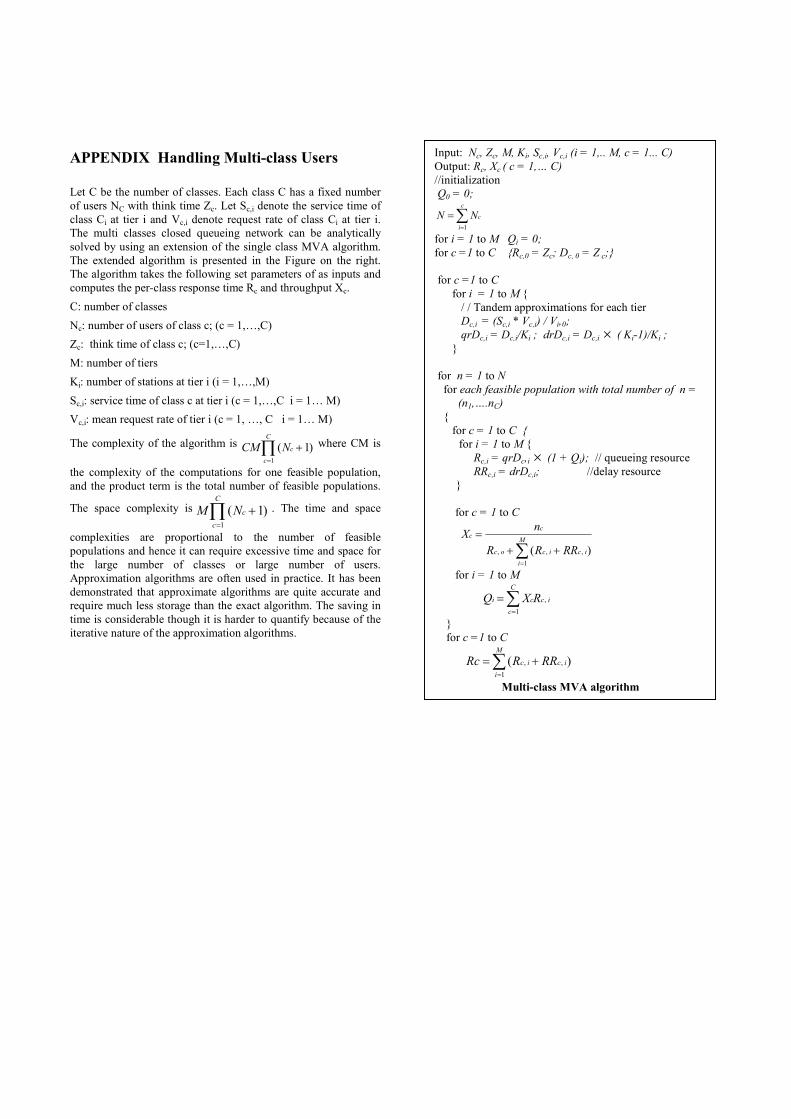
APPENDIX Handling Multi-class Users

Let C be the number of classes. Each class C has a fixed number

of users NC with think time Zc. Let Sc,i denote the service time of

class Ci at tier i and Vc,i denote request rate of class Ci at tier i.

The multi classes closed queueing network can be analytically

solved by using an extension of the single class MVA algorithm.

The extended algorithm is presented in the Figure on the right.

The algorithm takes the following set parameters of as inputs and

computes the per-class response time Rc and throughput Xc.

C: number of classes

Nc: number of users of class c; (c = 1,…,C)

Zc: think time of class c; (c=1,…,C)

M: number of tiers

Ki: number of stations at tier i (i = 1,…,M)

Sc,i: service time of class c at tier i (c = 1,…,C i = 1… M)

Vc,i: mean request rate of tier i (c = 1, …, C i = 1… M)

The complexity of the algorithm is ∏=

+C

c

cNCM1

)1( where CM is

the complexity of the computations for one feasible population,

and the product term is the total number of feasible populations.

The space complexity is ∏=

+C

c

cNM1

)1( . The time and space

complexities are proportional to the number of feasible

populations and hence it can require excessive time and space for

the large number of classes or large number of users.

Approximation algorithms are often used in practice. It has been

demonstrated that approximate algorithms are quite accurate and

require much less storage than the exact algorithm. The saving in

time is considerable though it is harder to quantify because of the

iterative nature of the approximation algorithms.