Chinese Journal of Aeronautics, (2014),27(4): 884–891

Chinese Society of Aeronautics and Astronautics& Beihang University

Chinese Journal of Aeronautics

cja@buaa.edu.cnwww.sciencedirect.com

Systematic centroid error compensation for

the simple Gaussian PSF in an electronic star map

simulator

* Corresponding author. Tel.: +86 10 68384574.

E-mail address: yonghai-wang@163.com (Y. Wang).

Peer review under responsibility of Editorial Committee of CJA.

Production and hosting by Elsevier

http://dx.doi.org/10.1016/j.cja.2014.03.0271000-9361 ª 2014 Production and hosting by Elsevier Ltd. on behalf of CSAA & BUAA. Open access under CC BY-NC-ND license.

Wang Haiyong a, Wang Yonghai b,*, Li Zhifeng c, Song Zhenfei a

a School of Astronautics, Beihang University, Beijing 100191, Chinab Beijing Institute of Space Long March Vehicle, Beijing 100076, Chinac National Key Laboratory of Science and Technology on Test Physics & Numerical Mathematics, Beijing 100076, China

Received 10 July 2013; revised 20 November 2013; accepted 10 February 2014Available online 18 March 2014

KEYWORDS

Error compensation;

Image analysis;

Point spread function;

Star map simulation;

Star sensor

Abstract Simulated star maps serve as convenient inputs for the test of a star sensor, whose stan-

dardability mostly depends on the centroid precision of the simulated star image, so it is necessary

to accomplish systematic error compensation for the simple Gaussian PSF (or SPSF, in which PSF

denotes point spread function). Firstly, the error mechanism of the SPSF is described, the reason of

centroid deviations of the simulated star images based on SPSF lies in the unreasonable sampling

positions (the centers of the covered pixels) of the Gaussian probability density function. Then in

reference to the IPSF simulated star image spots regarded as ideal ones, and by means of normal-

ization and numerical fitting, the pixel center offset function expressions are got, so the systematic

centroid error compensation can be executed simply by substituting the pixel central position with

the offset position in the SPSF. Finally, the centroid precision tests are conducted for the three big

error cases of Gaussian radius r = 0.5, 0.6, 0.671 pixel, and the centroid accuracy with the compen-

sated SPSF (when r = 0.5) is improved to 2.83 times that of the primitive SPSF, reaching a 0.008

pixel error, an equivalent level of the IPSF. Besides its simplicity, the compensated SPSF further

increases both the shape similarity and the centroid precision of simulated star images, which helps

to improve the image quality and the standardability of the outputs of an electronic star map sim-

ulator (ESS).ª 2014 Production and hosting by Elsevier Ltd. on behalf of CSAA & BUAA.Open access under CC BY-NC-ND license.

1. Introduction

A star map simulator generates standard artificial star maps asinputs for testing a star sensor. Currently there are two types ofstar simulator, one is physical starlight simulator, and the

other is electronic star map simulator (ESS). Star maps simu-lated by an ESS according to assigned nominal attitude can

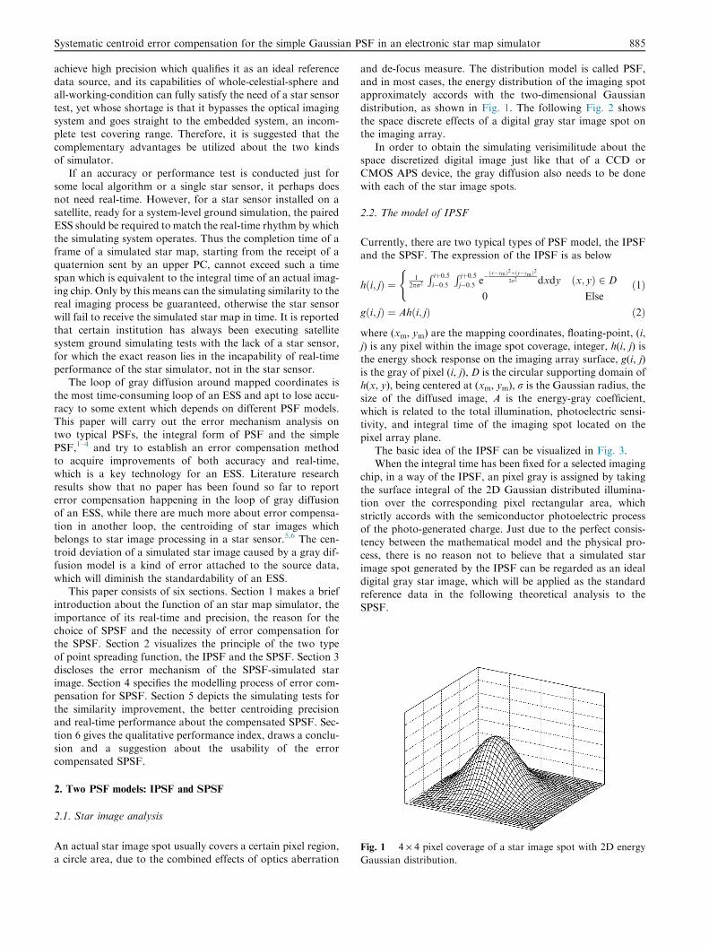
Fig. 1 4 · 4 pixel coverage of a star image spot with 2D energy

Gaussian distribution.

Systematic centroid error compensation for the simple Gaussian PSF in an electronic star map simulator 885

achieve high precision which qualifies it as an ideal referencedata source, and its capabilities of whole-celestial-sphere andall-working-condition can fully satisfy the need of a star sensor

test, yet whose shortage is that it bypasses the optical imagingsystem and goes straight to the embedded system, an incom-plete test covering range. Therefore, it is suggested that the

complementary advantages be utilized about the two kindsof simulator.

If an accuracy or performance test is conducted just for

some local algorithm or a single star sensor, it perhaps doesnot need real-time. However, for a star sensor installed on asatellite, ready for a system-level ground simulation, the pairedESS should be required to match the real-time rhythm by which

the simulating system operates. Thus the completion time of aframe of a simulated star map, starting from the receipt of aquaternion sent by an upper PC, cannot exceed such a time

span which is equivalent to the integral time of an actual imag-ing chip. Only by this means can the simulating similarity to thereal imaging process be guaranteed, otherwise the star sensor

will fail to receive the simulated star map in time. It is reportedthat certain institution has always been executing satellitesystem ground simulating tests with the lack of a star sensor,

for which the exact reason lies in the incapability of real-timeperformance of the star simulator, not in the star sensor.

The loop of gray diffusion around mapped coordinates isthe most time-consuming loop of an ESS and apt to lose accu-

racy to some extent which depends on different PSF models.This paper will carry out the error mechanism analysis ontwo typical PSFs, the integral form of PSF and the simple

PSF,1–4 and try to establish an error compensation methodto acquire improvements of both accuracy and real-time,which is a key technology for an ESS. Literature research

results show that no paper has been found so far to reporterror compensation happening in the loop of gray diffusionof an ESS, while there are much more about error compensa-

tion in another loop, the centroiding of star images whichbelongs to star image processing in a star sensor.5,6 The cen-troid deviation of a simulated star image caused by a gray dif-fusion model is a kind of error attached to the source data,

which will diminish the standardability of an ESS.This paper consists of six sections. Section 1 makes a brief

introduction about the function of an star map simulator, the

importance of its real-time and precision, the reason for thechoice of SPSF and the necessity of error compensation forthe SPSF. Section 2 visualizes the principle of the two type

of point spreading function, the IPSF and the SPSF. Section 3discloses the error mechanism of the SPSF-simulated starimage. Section 4 specifies the modelling process of error com-pensation for SPSF. Section 5 depicts the simulating tests for

the similarity improvement, the better centroiding precisionand real-time performance about the compensated SPSF. Sec-tion 6 gives the qualitative performance index, draws a conclu-

sion and a suggestion about the usability of the errorcompensated SPSF.

2. Two PSF models: IPSF and SPSF

2.1. Star image analysis

An actual star image spot usually covers a certain pixel region,a circle area, due to the combined effects of optics aberration

and de-focus measure. The distribution model is called PSF,and in most cases, the energy distribution of the imaging spotapproximately accords with the two-dimensional Gaussian

distribution, as shown in Fig. 1. The following Fig. 2 showsthe space discrete effects of a digital gray star image spot onthe imaging array.

In order to obtain the simulating verisimilitude about thespace discretized digital image just like that of a CCD orCMOS APS device, the gray diffusion also needs to be done

with each of the star image spots.

2.2. The model of IPSF

Currently, there are two typical types of PSF model, the IPSFand the SPSF. The expression of the IPSF is as below

hði; jÞ ¼1

2pr2

R iþ0:5i�0:5

R jþ0:5j�0:5 e

�ðx�xmÞ2þðy�ymÞ2

2r2 dxdy ðx; yÞ 2 D

0 Else

(ð1Þ

gði; jÞ ¼ Ahði; jÞ ð2Þ

where (xm, ym) are the mapping coordinates, floating-point, (i,

j) is any pixel within the image spot coverage, integer, h(i, j) isthe energy shock response on the imaging array surface, g(i, j)is the gray of pixel (i, j), D is the circular supporting domain of

h(x, y), being centered at (xm, ym), r is the Gaussian radius, thesize of the diffused image, A is the energy-gray coefficient,which is related to the total illumination, photoelectric sensi-tivity, and integral time of the imaging spot located on the

pixel array plane.The basic idea of the IPSF can be visualized in Fig. 3.When the integral time has been fixed for a selected imaging

chip, in a way of the IPSF, an pixel gray is assigned by takingthe surface integral of the 2D Gaussian distributed illumina-tion over the corresponding pixel rectangular area, which

strictly accords with the semiconductor photoelectric processof the photo-generated charge. Just due to the perfect consis-tency between the mathematical model and the physical pro-

cess, there is no reason not to believe that a simulated starimage spot generated by the IPSF can be regarded as an idealdigital gray star image, which will be applied as the standardreference data in the following theoretical analysis to the

SPSF.

Fig. 2 A space discretized digital gray star image spot.

Fig. 3 Visualized schematic of the IPSF.

Fig. 4 Visualized schematic of the SPSF.

886 H. Wang et al.

2.3. The model of SPSF

The second PSF type is the simple PSF (SPSF), whose expres-sion is described as follows

g2ði; jÞ ¼B

2pr2exp �ði� xmÞ2 þ ðj� ymÞ

2

2r2

!ð3Þ

where the meanings of (i, j), (xm, ym) and r are the same as in

Eq. (1), B is the energy-gray coefficient of the SPSF, but thepixel gray assignment of the SPSF is different, derived fromthe directly sampled value of the Gaussian probability density

function just at the pixel center, as shown in Fig. 4.The SPSF has such advantages as simplicity and real-time

due to no integration and less computing, but unfortunatelyits drawback is its inherent systematic error, which is related

with the Gaussian radius r and the deviation of the mappinglocation (floating-point type) from the integer pixel center.

2.4. Real-time performance and model selection

As for real-time, it is a prerequisite to determine whether a starmap simulator can be incorporated into a ground real-time

simulating system to execute in-system dynamic simulation.If a process of star map simulating could finish all the comput-ing in a period shorter than the equivalent integration time

(e.g., 50 ms) of an actual imaging chip, in the end at a readystate for outputting, what the simulator achieves can be called

ultra-real-time simulating, which means that it is fully capableof outputting simulated star maps with a frame frequency not

lower than the actual imaging chip; similarly, the case of equaltime corresponds to real-time simulating; longer computingtime than the integration time corresponds to sub-real-time.7

At present, an implementation of real-time or ultra-real-

time simulation is not so easy because each star in a simulatedstar map needs to have coordinate mapping and gray diffusiondone, which means a great deal of computation. According to

Ref. 8, the computing time of one simulated static star map is63 ms, already saving 1.118 s compared with the ordinaryOpenGL simulating method (1.281 s), and please note that

the performance level was achieved only when the new technol-ogy of GPU hardware process was adopted. But even so, thelevel of 63 ms is just enough for a real-time simulating

requirement.Therefore, from the perspective of time saving and based on

the self-evident truth that a simple model may lead to reduc-tion in calculation, the non-integral SPSF is usually preferred

than the IPSF just due to its simplicity and can satisfy therequirement of real-time or even ultra-real-time for an ESS.

3. Error mechanism of the SPSF-simulated star image

In order to let the sets of pixel gray by the two models (IPSFand SPSF) be comparable, normalized mathematical analysis

is adopted.9 Since the illumination and optical integration timeis the same, if no model error, the gray peak value should bethe same even though different models. This idea is virtually

the rational basis for the normalization.First of all, for the IPSF, a 2D Gaussian illumination func-

tion is established in such a way that it is symmetrically distrib-

uted about the center of a pixel. Let the integral value over theexact central pixel area correspond to the full-scale gray (i.e.,255 for 8 bit AD, 1023 for 10 bit AD). In this case, the centralpixel integral value is defined as unit 1, namely the normalized

unit 1 quantization value of the IPSF

UI ¼Amax

2pr2

Z 0:5

�0:5

Z 0:5

�0:5e�x2þy2

2r2 dxdy ð4Þ

where Amax is the gray coefficient used to adjust to the full-scale gray. Next, for star imaging spots in other cases, i.e., withthe Gaussian symmetric center deviating from the pixel center,

or with gray not reaching the full scale, or with the combinedeffects of the above two, any pixel within the spot coverage canbe assigned a normalized value, namely the ratio of pixel grayto UI

Systematic centroid error compensation for the simple Gaussian PSF in an electronic star map simulator 887

gIði; jÞ ¼A

2pr2

R i�icþ0:5i�ic�0:5

R j�jcþ0:5j�jc�0:5

e�ðx�DxmÞ2þðy�DymÞ2

2r2 dxdy

UI

¼AR i�ðicþDxmÞþ0:5i�ðicþDxmÞ�0:5

R j�ðjcþDymÞþ0:5j�ðjcþDymÞ�0:5

e�x2þy2

2r2 dxdy

Amax

R 0:5

�0:5R 0:5

�0:5 e�x2þy2

2r2 dxdy

¼ A

Amax

�R i�ðicþDxmÞþ0:5i�ðicþDxmÞ�0:5 e

� x2

2r2dxR 0:5

�0:5 e� x2

2r2dx�R j�ðjcþDymÞþ0:5j�ðjcþDymÞ�0:5

e� y2

2r2dyR 0:5

�0:5 e� y2

2r2dyð5Þ

where the central integer coordinates (ic, jc) are acquired by around-off of the star mapping coordinates (xm, ym) of floating-

point type. Hence, xm = ic + Dxm, ym = jc + Dym, unit: pixel.Eq. (5) can be disassembled into two parts according to theindependence of x and y of a 2D Gaussian distribution

function.Secondly, to set up the normalized method of the SPSF, the

quantized value of unit 1 is defined as the full-scale gray, whichis transformed from the maximum value of the Gaussian prob-

ability density function of illumination. If the Gaussian distri-bution is symmetrical about a pixel, the normalized valuecorresponds to the peak value sampled exactly at the center

of the central pixel

US ¼Bmax

2pr2ð6Þ

where Bmax is the gray-energy coefficient of the SPSF. Next,the normalized gray value of an arbitrary pixel within the cov-

erage of a star image spot is

gsði; jÞ ¼B

2pr2 e�ði�ic�DxmÞ2þðj�jc�DymÞ2

2r2

Us

¼ B

Bmax

e� i�ðicþDxmÞ½ �2

2r2 � e�j�ðjc�DymÞ½ �2

2r2 ð7Þ

Let the equation A/Amax = B/Bmax be true irrespective of

the model difference, even so, the normalized gray valuesobtained by the IPSF and the SPSF respectively are still incon-sistent, for which the exact reason lies not in B/Bmax but in thecentral sampling coordinates (i, j) of Eq. (7). It is indeed just

like that, and some adverse consequences occur. Firstly, twosets of assigned gray values within the coverage of the starimage spot are different between the two models; secondly,

the ultimate calculated centroid of the SPSF-simulated starimage spot will deviate from the ideal mapped centralcoordinates.

The error mechanism is that the SPSF-assigned pixel gray isderived from the sampled value of the 2D Gaussian probabil-ity density function just at the center of the pixel (an unreason-able sampling location), in addition that a Gaussian surface is

nonlinear, resulting in the deviation from the ideal mappedcentral coordinates.

4. Modeling for the error compensated SPSF

According to the above analysis about Eq. (7), some compen-sation measures should be adopted to equate the normaliza-

tion value by the SPSF to that of the IPSF, fully conformingto the assigned gray distribution of the IPSF-simulated starimage spot, which possesses perfect similarity to a real shot

star image because of the completeness of the IPSF model.Out of this idea, Eq. (7) is modified as follows

gSði; jÞ ¼B

Bmax

� e�ðiþDi Þ�ðicþDxmÞ½ �2

2r2 � e�ðjþDjÞ�ðjcþDymÞ½ �2

2r2

¼ B

Bmax

� e�ði�xmþDiÞ2

2r2 � e�ðj�ymþDjÞ2

2r2 ð8Þ

where two offset items Di and Dj are inserted to the object pixel(i, j), which are the central coordinates of the object pixel, inte-ger type. As a result, the normalized gray of pixel (i, j) is eval-

uated according to the sampled value of the 2D Gaussianfunction at position (i + Di, j + Dj), not the central position(i, j), just aiming to acquire equal normalization values

between the two models. The task of error compensation mod-eling is virtually to set up a function expression of the offsetitems (Di, Dj) with regard to the Gaussian radius r and thedistance (i � xm, j � ym) from the object pixel center to the

mapping location.Since this is a modeling process, and considering that

A/Amax = B/Bmax, let the corresponding parts of the two

Eqs. (5) and (8) be equal to each other

e� i�xmþDið Þ2

2r2 ¼R i�xmþ0:5

i�xm�0:5e� x2

2r2 dxR 0:5

�0:5e� x2

2r2 dx

e�

j�ymþDjð Þ22r2 ¼

R j�ymþ0:5

j�ym�0:5e� y2

2r2 dyR 0:5

�0:5e� y2

2r2 dy

8>>>>>><>>>>>>:

ð9Þ

The right-hand parts of Eq. (9) are written respectively asRx(i � xm, r) and Ry(j � ym, r), and then the above Eq. (9)can be transformed into

Di¼�ði�xmÞþ

ffiffiffiffiffiffiffiffiffiffiffiffiffiffiffiffiffiffiffiffiffiffiffiffiffiffiffiffiffiffiffiffiffiffiffiffiffiffiffiffiffi�2r2 lnRxði�xm;rÞ

pIf i�xm� 0

�ði�xmÞ�ffiffiffiffiffiffiffiffiffiffiffiffiffiffiffiffiffiffiffiffiffiffiffiffiffiffiffiffiffiffiffiffiffiffiffiffiffiffiffiffiffi�2r2 lnRyði�xm;rÞ

pIf i�xm< 0

8<: ð10Þ

Di¼�ði�xmÞþ

ffiffiffiffiffiffiffiffiffiffiffiffiffiffiffiffiffiffiffiffiffiffiffiffiffiffiffiffiffiffiffiffiffiffiffiffiffiffiffiffiffi�2r2 lnRxði�xm;rÞ

pIf i�xm� 0

�ði�xmÞ�ffiffiffiffiffiffiffiffiffiffiffiffiffiffiffiffiffiffiffiffiffiffiffiffiffiffiffiffiffiffiffiffiffiffiffiffiffiffiffiffiffi�2r2 lnRyði�xm;rÞ

pIf i�xm< 0

8<: ð11Þ

where the above two expressions about rows and columns

respectively are apparently of the same appearance, thereforethe simulation test and analysis can be carried out just byselecting the row function Di = f(i � xm, r), whose parameterfitting process wholly applies to the column function Dj.

Set the pixel coordinates (ic, jc) to (0, 0), analyzing from �6to 6 altogether 13 pixels on both sides of the origin 0 along therow direction. 10 offset values, which represent the deviation

values of i � xm, are sampled at a step of 0.1 pixel in the inter-val [�0.5, 0.5) pixel. Then, the function values of Di withregard to i � xm and r have such a 3D distribution figure as

in Fig. 5.A family of function curves about Di and i � xm under dif-

ferent r values can also be obtained as shown in Fig. 6.

For Nos. (�1) and (�2) pixels, when the mapping deviationDxm equals to 0.2 pixel, the variation curves of function Di

against the Gaussian radius r are plotted in Fig. 7.Based on the simulated data of Eq. (10), function Di can be

surface fitted. The kernel functions about variable x (represent-ing i � xm) may be selected as x and x3 because of its odd sym-metry about the origin. The other kernel functions about

variable r can be selected as 1, r, r2.As a result of least square surface fitting with 3D data

(i � xm, r, Di), the coefficient matrix is calculated as follows10

Fig. 5 3D figure of the offset values Di with regard to i � xm and

r.

Fig. 6 Function curves of offset value Di with regard to i � xmunder different r.

888 H. Wang et al.

C ¼c00 c01 c02

c10 c11 c12

� �¼�0:2030 0:2260 �0:06650:0030 �0:0041 0:0013

� �ð12Þ

The final fitting equation of Di is got as below

Di ¼ ½x; x3�C1

r

r2

264

375 ð13Þ

where x represents the item (i � xm).After comparison analysis of the two computation results

from Eqs. (10) and (13), the global fitting accuracy about Di is

Fig. 7 Two function curves of offset value Di against r(Dxm ¼ 0:2pixel).

rDi¼

ffiffiffiffiffiffiffiffiffiffiffiffiffiffiffiffiffiffiffiffiffiffiffiffiffiffiffiffiffiffiffiffiffiffiffiffiffiffiffiffiffiffiffiffiffiffiffiffiffiffiffiffiffiffiffiffiffiffiffiffiffiffiffiffiffiffiffiffiffiffiffiffiffiffiffiffiffiffiffiffiffiffiffi1

17� 130

X17k¼1

X130j¼1

Di ði� xmÞj; rk

� �� Di

h i2vuut¼ 0:0019pixel ð14Þ

For the particular case of r = 0.671 pixel, characterized bythat more than 95% of star image energy is distributed in a

3 · 3 pixels coverage, the necessary pixels to be treated are atleast 4 · 4 pixels. In the domain of (i � xm) 2 [�4.4, 4.5], theprobable location range of the effective distance from the

object pixel center to the mapping x coordinate, its 1D localfitting accuracy of Eq. (13) under the case of r = 0.671 isobtained as below

r0Di¼

ffiffiffiffiffiffiffiffiffiffiffiffiffiffiffiffiffiffiffiffiffiffiffiffiffiffiffiffiffiffiffiffiffiffiffiffiffiffiffiffiffiffiffiffiffiffiffiffiffiffiffiffiffiffiffiffiffiffiffiffiffiffiffiffiffiffiffi1

90

X110j¼21

Diðði� xmÞj; r0:671Þ � Di

h i2vuut ¼ 0:0018pixel ð15Þ

Under the cases of r = 0.5, 0.7, 0.9, each of the functionalcurves and its corresponding fitted curve are plotted respec-

tively in Fig. 8.Because of the equivalence of x and y axes of the 2D Gauss-

ian distribution, the coefficient matrix C in Eq. (13) can be

directly copied to the function expression Dj. Finally, the val-ues of Di and Dj based on Eq. (13) are plugged into Eq. (8),which fulfills the gray error compensation for the SPSF.

5. Simulating test for the compensated SPSF

In view of the self-evident truth that a simple model is boundto boost the simulating speed, so real-time performance is not

the test task here, and only the item of precision is chosen andwill be tested in the following procedures. As for the selectionof a test tool, there are no better verifying tools than the sim-

ulating tool. For a real shot star image, there is no way toobtain its ideal centroid and no way to conduct an erroranalysis.

5.1. Similarity improvement test

One cannot tell tiny gray differences between image pictures by

naked eyes, so it is more meaningful to give the gray data forcomparison than to list the star images simulated by the threemodels of the SPSF, the compensated SPSF, and the IPSF.

Fig. 8 Three cases of functional curves and their fitted curves.

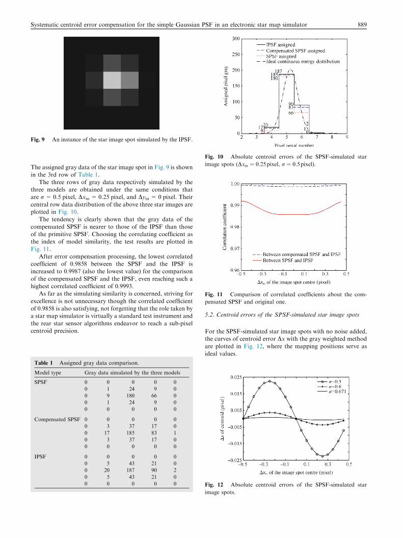
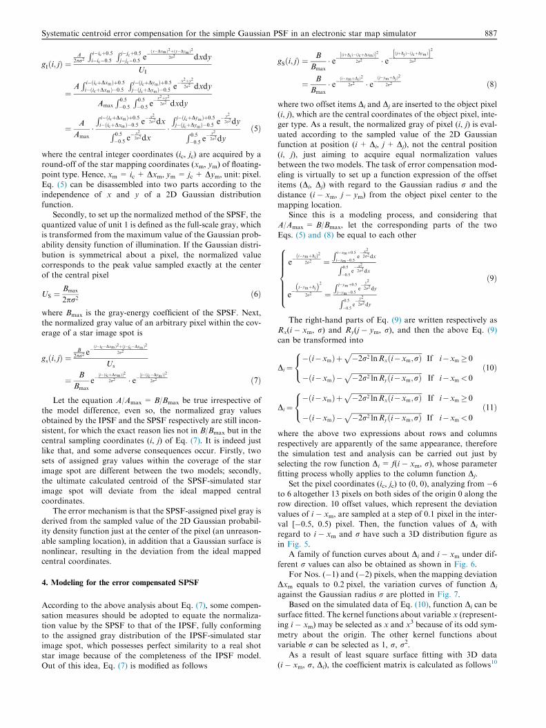
Fig. 9 An instance of the star image spot simulated by the IPSF.

Fig. 10 Absolute centroid errors of the SPSF-simulated star

image spots (Dxm ¼ 0:25pixel, r ¼ 0:5pixel).

Fig. 11 Comparison of correlated coefficients about the com-

pensated SPSF and original one.

Systematic centroid error compensation for the simple Gaussian PSF in an electronic star map simulator 889

The assigned gray data of the star image spot in Fig. 9 is shown

in the 3rd row of Table 1.The three rows of gray data respectively simulated by the

three models are obtained under the same conditions thatare r = 0.5 pixel, Dxm = 0.25 pixel, and Dym = 0 pixel. Their

central row data distribution of the above three star images areplotted in Fig. 10.

The tendency is clearly shown that the gray data of the

compensated SPSF is nearer to those of the IPSF than thoseof the primitive SPSF. Choosing the correlating coefficient asthe index of model similarity, the test results are plotted in

Fig. 11.After error compensation processing, the lowest correlated

coefficient of 0.9858 between the SPSF and the IPSF isincreased to 0.9987 (also the lowest value) for the comparison

of the compensated SPSF and the IPSF, even reaching such ahighest correlated coefficient of 0.9993.

As far as the simulating similarity is concerned, striving for

excellence is not unnecessary though the correlated coefficientof 0.9858 is also satisfying, not forgetting that the role taken bya star map simulator is virtually a standard test instrument and

the rear star sensor algorithms endeavor to reach a sub-pixelcentroid precision.

Table 1 Assigned gray data comparison.

Model type Gray data simulated by the three models

SPSF 0 0 0 0 0

0 1 24 9 0

0 9 180 66 0

0 1 24 9 0

0 0 0 0 0

Compensated SPSF 0 0 0 0 0

0 3 37 17 0

0 17 185 83 1

0 3 37 17 0

0 0 0 0 0

IPSF 0 0 0 0 0

0 5 43 21 0

0 20 187 90 2

0 5 43 21 0

0 0 0 0 0

5.2. Centroid errors of the SPSF-simulated star image spots

For the SPSF-simulated star image spots with no noise added,the curves of centroid error Dx with the gray weighted methodare plotted in Fig. 12, where the mapping positions serve as

ideal values.

Fig. 12 Absolute centroid errors of the SPSF-simulated star

image spots.

Fig. 13 Absolute centroid errors of the IPSF star image spots.

Fig. 14 Absolute centroid errors of the compensated SPSF

simulated star image spots.

890 H. Wang et al.

It can be seen that the centroid error eminently increases asthe Gaussian radius r decreases. When r = 0.5 pixel, the max-imum absolute error reaches up to 0.0226 pixel (at

Dxm =±0.25 pixel), larger than 1/50 pixel, a non-negligiblelevel, but when r = 0.671, the maximum absolute error ismerely 0.0008 pixel, that is to say, if the Gaussian radius rof the simulated star image spot is greater than 0.671 pixel,there is no need for the SPSF to adopt a compensation mea-sure, because it does not matter to use it directly; if not, thatturns to be necessary.

5.3. Centroid error of the IPSF-simulated star image spots

The absolute centroid error curves of the IPSF-simulated star

image spots are shown in Fig. 13.Though it is similar to that of the SPSF in Fig. 12 by out-

ward appearance, its maximum absolute error is merely 0.0023

Table 2 Consumed time of the 3 PSFs.

Model type 1st 2nd

IPSF(s) 14.27 14.32

SPSF(ms) 54.3 53.6

Compensated SPSF(ms) 61.7 62.4

pixel at Dxm =±0.25 pixel when r = 0.5 pixel, an order oferror magnitude far lower than that of the SPSF, which iswhy the offset compensation method for the SPSF is set up

through numerical fitting in reference to the gray values gener-ated by the IPSF.

5.4. Centroid error of the compensated SPSF simulated starimage spots

With no noise added to star image spots simulated by the com-

pensated SPSF, absolute centroid error curves with the grayweighted method are plotted in Fig. 14.

In comparison with Figs. 13 and 14, all of them reach up to

the same 10�3 pixel order of magnitude about their absolutemaximum centroid errors, as well as with similar forms. Fur-thermore, compared with centroid error of the SPSF shownin Fig. 12, under the same condition of r = 0.5 and at

Dxm =± 0.25 pixel, the absolute maximum centroid errorof the compensated SPSF in Fig. 14 is only 0.008 pixel, a2.83-times accuracy in comparison to the primitive SPSF,

which manifests the validity of the offset compensated methodfor the SPSF.

5.5. Real-time performance tests

After observing qualitatively the three expressions of the PSF,namely the IPSF expressed by Eqs. (1) and (2), the SPSF byEq. (6), and the compensated SPSF by Eq. (8), such a judg-

ment can be made that the computational time of the IPSFhas to be far more than those of the SPSFs because of itsinvolved integral function, and that the compensated SPSF

will also consume a bit more time than the primitive SPSF justfor the extra computation about Di and Dj expressed byEqs. (10) and (11).

The real-time performance comparison tests were con-ducted under the following hardware and software simulatingcircumstances: Intel Duo CPU P8600@2.40 GHz, Win7 64 bit,

and Matlab 2010a. A pair of mapped coordinates on theimaging array were assumed at (200.45, 200.45), around whichgray diffusion was executed according to the 3 PSFs toconstruct a simulated star image, and 100 times of repetitive

computation were operated for each PSF in order to reachan equivalent amount of computation as that of a simulatedstar map which contained 100 stars inside. The elapsed time

was counted respectively for the three cases of PSF, as shownin Table 2.

As expected, the consumed time of the IPSF (mean value of

14.3 s) is 2 orders of magnitude more than the latter twoSPSFs, which simply cannot satisfy the requirement of real-time simulating tests. The involved double integral function

(dblquad() in the Matlab program) actually uses the methodof recursive adaptive Simpson quadrature which is doomedto consume more computations.

3rd 4th 5th Mean

14.37 14.30 14.21 14.30

53.5 53.4 53.1 53.6

61.7 61.4 61.8 61.8

Systematic centroid error compensation for the simple Gaussian PSF in an electronic star map simulator 891

As for the compensated SPSF, its consumed time has asmall difference of 8.2 ms by reference to the time of the prim-itive SPSF, just caused by the extra computation about Di and

Dj, yet the final better centroiding precision is worthy of thatexchange of time price. To a star sensor mounted in a satelliteground real-time simulating test system, its paired electronic

star map simulator must keep up with data updating fre-quency, and this level of time consumed by the SPSF or thecompensated one is sufficient to meet with the demand for

the output rate (higher than 10 Hz in general).

6. Conclusions

(1) The SPSF has such advantages as simplicity and fewer

computations, and therefore good real-time, but hasinherent systematic error. Its error mechanism is thatthe SPSF-assigned pixel gray derives from the sampled

value of the 2D Gaussian probability density functionjust at the center of the pixel (an unreasonable position),in addition to that the surface of a Gaussian distribution

is nonlinear, which results in a deviation from the idealpredefined mapping coordinates.

(2) In reference to the IPSF-simulated star image, the offsetfunctions Di and Dj from the pixel center are got, which

are of the two variables i � xm and r, and subsequentlythe systematic error compensation for the SPSF is exe-cuted by substituting the pixel central position (i, j) with

the offset position (i + Di, j + Dj). In the simulationtests, for the big error case of r = 0.5 pixel, the compen-sated SPSF achieves an improved similarity, almost

wholly compensated for the centroid systematic error(the maximum error is 0.0226 pixel, larger than 1/50pixel) of the primitive SPSF, reaching a 0.008 pixel max-

imum error level, a 2.83-times precision in comparisonto the primitive SPSF.

(3) The lower the r value, the worse situation of the system-atic error, so it is suggested that the compensation mea-

sure for the SPSF be adopted when r < 0.671 pixel, insuch a manner the standardability of star map outputsof an electronic or software simulator can be insured.

However, when r > 0.671 pixel (a dividing value for ref-erence only), the compensating effects are not thatprominent.

References

1. Liebe CC. Accuracy performance of star trackers-a tutorial. IEEE

Trans Aerosp Electron Sys 2002;38(2):587–99.

2. Gao Y, Lin ZP, Li J, An W, Xu H. Imaging simulation algorithm

for star field based on CCD PSF and space target’s striation

characteristic. Electron Inf Warfare Technol 2008;23(2):58–62

[Chinese].

3. Wang HY, Fei ZH, Wang XL. Precise simulation of star spots and

centroid computation based on Gaussian distribution. Opt Precis

Eng 2009;17(7):1672–7 [Chinese].

4. Wang HY, Zhou WR, Zhao YW. Error analysis and applicability

study on the simplified Gaussian gray diffusion model. Acta Opt

Sin 2012;32(7):0711002 [Chinese].

5. Yang J, Zhang T, Song JY, Liang B. High accuracy error

compensation algorithm for star image sub-pixel sub-division

location. Opt Precis Eng 2010;18(4):1002–9 [Chinese].

6. Jia H, Yang JK, Li XJ, Yang JC, Yang MF, Liu YW, et al.

Systematic error analysis and compensation for high accuracy star

centroid estimation of star tracker. Sci China Technol Sci

2010;53(11):3145–52.

7. Xiao TY, Zhang YY, Chen JD. Introduction to system simulation.

1st ed. Beijing: Tsinghua University Press; 2000. p. 5–6 [Chinese].

8. Shi QS, Lan CZ, Xu Q, Zhou Y, Liu ZQ. Rapid star map

simulation based on GPU. In: 2010 International Conference on

Audio Language and Image Processing (ICALIP); 2010 November

23–25; Shanghai, China; 2010. p. 638–42.

9. Wen YM, Zhao XM, Li P, Wen J, Zhang M. Modification of light

emitting diode’s normalized spectrum model. Acta Ootica Sin

2012;32(1):0130001 [Chinese].

10. Yan QJ. Numerical analysis. Beijing: Beihang University Press;

2006 [Chinese].

Wang Haiyong received his Ph.D. degree in the speciality of Precision

Instruments and Machinery in 2004 from Beihang University, Beijing,

China, a lecturer for the course of Celestial Navigation Basis in the

School of Astronautics, Beihang University. More than 30 acadamic

papers have been published by him as the 1st author, and 2 invention

patents were granted as the 1st inventor. His research interests include:

celestial body sensor, celestial navigation and integrated navigation

system.

Wang Yonghai received his M.S. degree in 2003 in Automatic and

Electronic Engineering from Beihang University, Beijing, China. He is

currently a senior engineer with Beijing Institute of Space Long March

Vehicle, China. His research interests include numerical modeling,

design of circuits, and optoelectronic system.