system-level structural reliability of bridges · system-level structural reliability of ......
TRANSCRIPT

System-Level Structural Reliability of Bridges
by
Negar Elhami Khorasani
A thesis submitted in conformity with the requirements
for the degree of Master of Applied Science
Graduate Department of Civil Engineering
University of Toronto
© Copyright by Negar Elhami Khorasani (2010)

System-Level Structural Reliability of Bridges
Negar Elhami KhorasaniMaster of Applied ScienceGraduate Department of Civil EngineeringUniversity of Toronto
Abstract
e purpose of this thesis is to demonstrate that two-girder or two-web structural systems can be
employed to design efficient bridges with an adequate level of redundancy. e issue of redundancy in
two-girder bridges is a constraint for the bridge designers in North America who want to take advantage
of efficiency in this type of structural system. erefore, behavior of two-girder or two-web structural
systems aer failure of one main load-carrying component is evaluated to validate their safety. A
procedure is developed to perform system-level reliability analysis of bridges. is procedure is applied to
two bridge concepts, a twin steel girder with composite deck slab and a concrete double-T girder with
unbonded external tendons. e results show that twin steel girder bridges can be designed to ful'll the
requirements of a redundant structure and the double-T girder with external unbonded tendons can be
employed to develop a robust structural system.
ii

Acknowledgement
is work was partially funded through a scholarship from the National Science and Engineering
Research Council of Canada. eir support is greatly acknowledged.
I would like to express my sincere gratitude to my supervisor, Professor Paul Gauvreau for his
constructive comments and valuable support throughout this work. is thesis is the result of his
supervision, thoughtful guidance and encouragement.
I would also like to thank my research colleagues who helped and encouraged me throughout my studies:
Davis Doan, Kris Mermigas, Andrew Lehan, Eileen Li, Sandy Poon, Jason Salonga, Jeff Smith and Nick
Zwerling.
Finally, my special thanks goes to my parents and my sister for their endless love and support. I am truly
grateful to them for their patience throughout these years.
iii
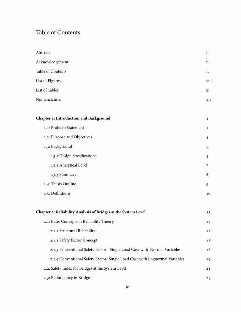
Table of Contents
Abstract ii
Acknowledgement iii
Table of Contents iv
List of Figures viii
List of Tables xi
Nomenclature xiv
Chapter : Introduction and Background
.: Problem Statement
.: Purpose and Objectives
.: Background
..:Design Speci'cations
..:Analytical Level
..:Summary
.: esis Outline
.: De'nitions
Chapter : Reliability Analysis of Bridges at the System Level
.: Basic Concepts in Reliability eory
..:Structural Reliability
..:Safety Factor Concept
..:Conventional Safety Factor - Single Load Case with Normal Variables
..:Conventional Safety Factor- Single Load Case with Lognormal Variables
.: Safety Index for Bridges at the System Level
.: Redundancy in Bridges
iv

Chapter : Bridge Load Models
.: Dead Load Model
.: Live Load Model for Bridges with Two-Traffic Lanes
..:Expected Maximum Truck Weights
..:Multiple Truck Presence
..:Transverse Position of Trucks
..:Possible Live Load Cases for Bridges with Two Lanes of Traffic
..:Probability of Occurrence for Live Load Events
.: Live Load Model for Bridges with ree-Traffic Lanes
.: Dynamic Effect of Live Load
.: Expected Live Loads in the Safety Index Formula
Chapter : e Acceptable Probability of Failure
.: Joint Committee of Structural Safety (JCSS) Provisions
..:Human Safety Approach - Individual Risk
..:Human Safety Approach - Societal Risk
..:Cost-Bene't Analysis
.: Eurocode Provisions
.: International Organization for Standardization
.: e NCHRP Report No. Guidelines
.: Acceptable Level of Redundancy
Chapter : Summary of Guidelines to Evaluate Redundancy of Bridges
.: Step-by-Step Procedure to Calculate Redundancy of Bridges at the System Level
.: Flowchart of Procedure to Calculate Redundancy of Bridges at the System Level
v
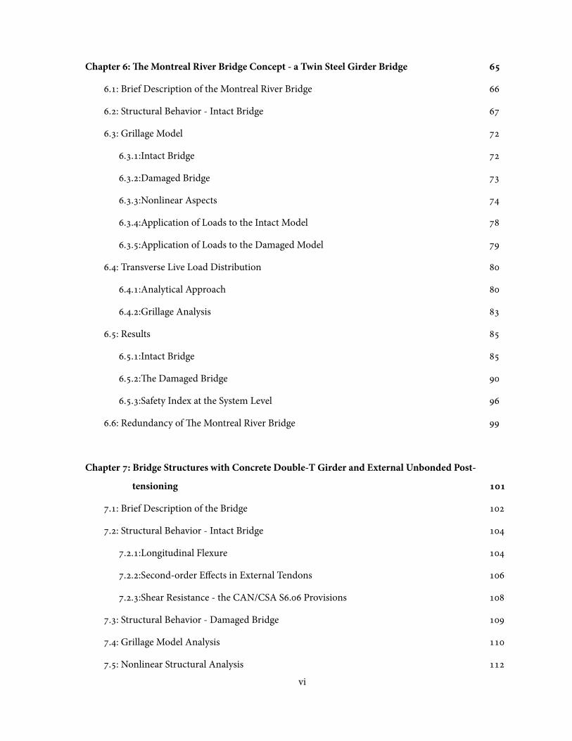
Chapter : e Montreal River Bridge Concept - a Twin Steel Girder Bridge
.: Brief Description of the Montreal River Bridge
.: Structural Behavior - Intact Bridge
.: Grillage Model
..:Intact Bridge
..:Damaged Bridge
..:Nonlinear Aspects
..:Application of Loads to the Intact Model
..:Application of Loads to the Damaged Model
.: Transverse Live Load Distribution
..:Analytical Approach
..:Grillage Analysis
.: Results
..:Intact Bridge
..:e Damaged Bridge
..:Safety Index at the System Level
.: Redundancy of e Montreal River Bridge
Chapter : Bridge Structures with Concrete Double-T Girder and External Unbonded Post-
tensioning
.: Brief Description of the Bridge
.: Structural Behavior - Intact Bridge
..:Longitudinal Flexure
..:Second-order Effects in External Tendons
..:Shear Resistance - the CAN/CSA S. Provisions
.: Structural Behavior - Damaged Bridge
.: Grillage Model Analysis
.: Nonlinear Structural Analysis
vi
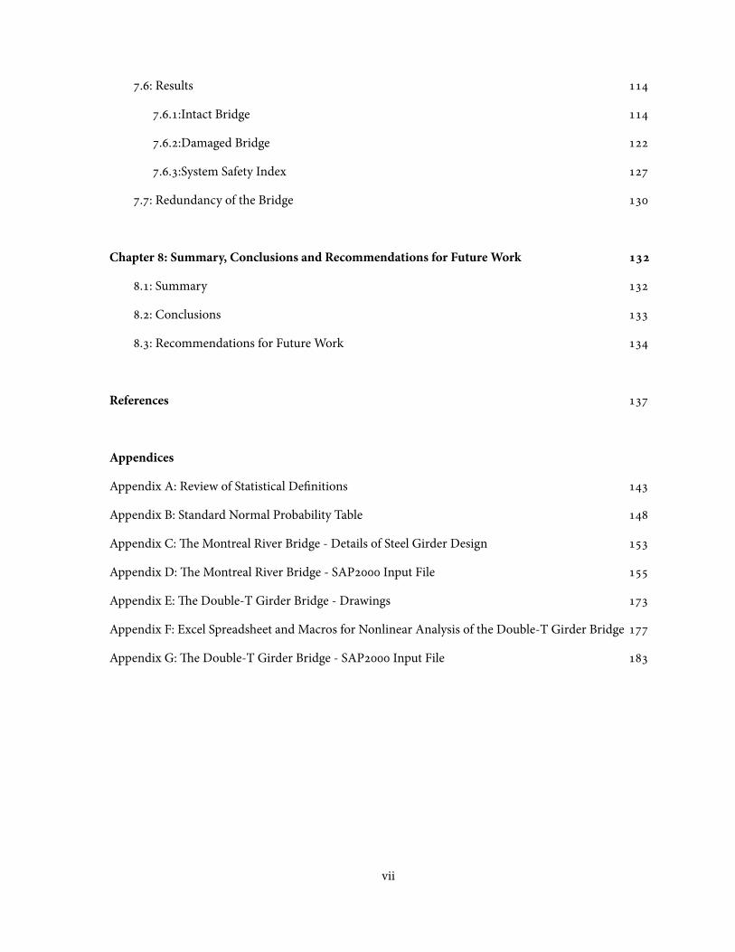
.: Results
..:Intact Bridge
..:Damaged Bridge
..:System Safety Index
.: Redundancy of the Bridge
Chapter : Summary, Conclusions and Recommendations for Future Work
.: Summary
.: Conclusions
.: Recommendations for Future Work
References
Appendices
Appendix A: Review of Statistical De'nitions
Appendix B: Standard Normal Probability Table
Appendix C: e Montreal River Bridge - Details of Steel Girder Design
Appendix D: e Montreal River Bridge - SAP Input File
Appendix E: e Double-T Girder Bridge - Drawings
Appendix F: Excel Spreadsheet and Macros for Nonlinear Analysis of the Double-T Girder Bridge
Appendix G: e Double-T Girder Bridge - SAP Input File
vii
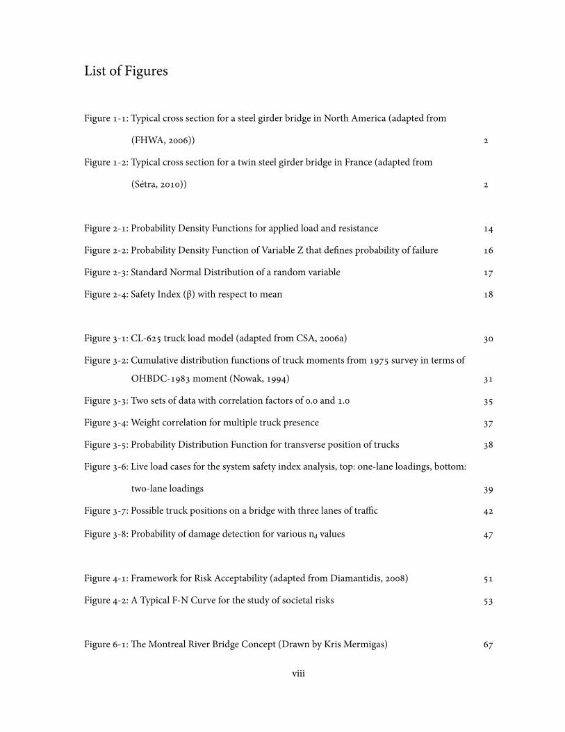
List of Figures
Figure -: Typical cross section for a steel girder bridge in North America (adapted from
(FHWA, ))
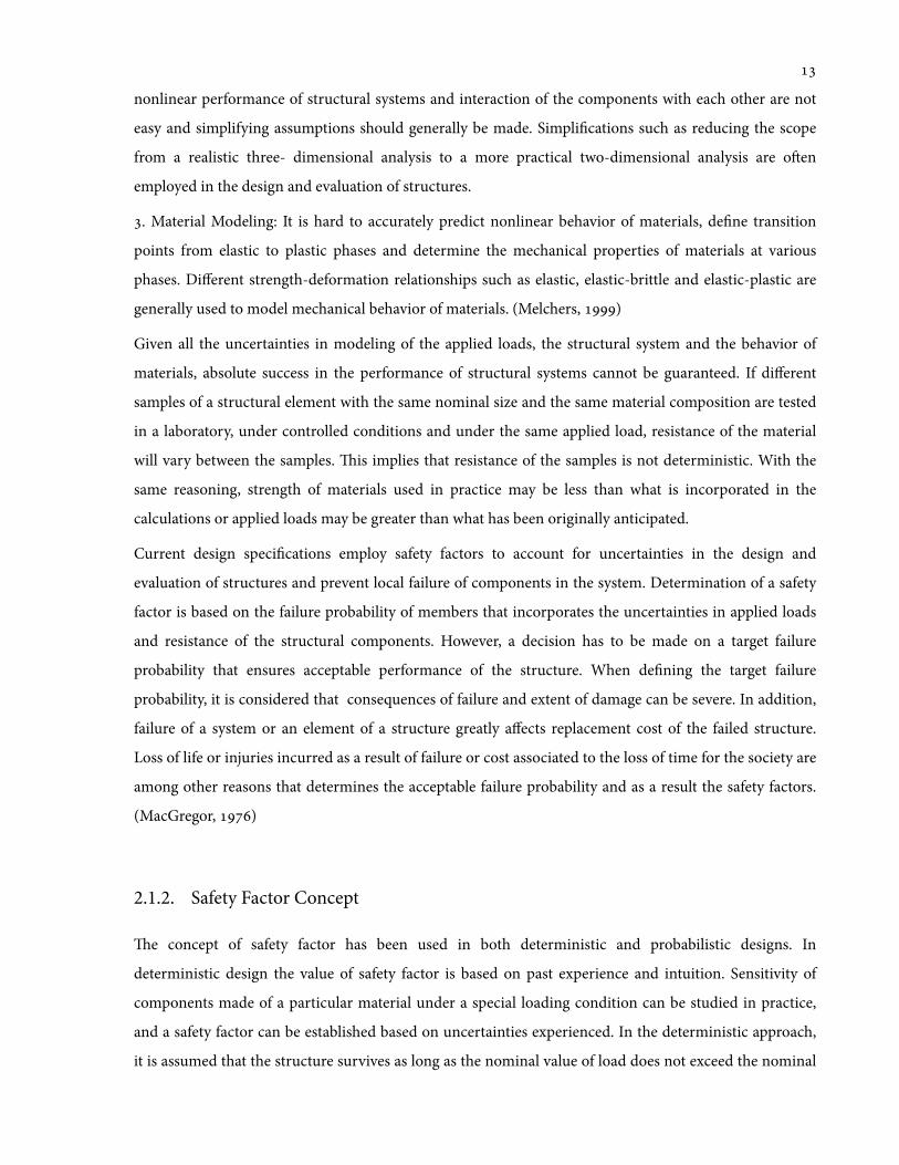
Figure -: Typical cross section for a twin steel girder bridge in France (adapted from
(Sétra, ))
Figure -: Probability Density Functions for applied load and resistance
Figure -: Probability Density Function of Variable Z that de'nes probability of failure
Figure -: Standard Normal Distribution of a random variable
Figure -: Safety Index (β) with respect to mean
Figure -: CL- truck load model (adapted from CSA, a)
Figure -: Cumulative distribution functions of truck moments from survey in terms of
OHBDC- moment (Nowak, )
Figure -: Two sets of data with correlation factors of . and .
Figure -: Weight correlation for multiple truck presence
Figure -: Probability Distribution Function for transverse position of trucks
Figure -: Live load cases for the system safety index analysis, top: one-lane loadings, bottom:
two-lane loadings
Figure -: Possible truck positions on a bridge with three lanes of traffic
Figure -: Probability of damage detection for various nd values
Figure -: Framework for Risk Acceptability (adapted from Diamantidis, )
Figure -: A Typical F-N Curve for the study of societal risks
Figure -: e Montreal River Bridge Concept (Drawn by Kris Mermigas)
viii

Figure -: Moment-Curvature diagram at mid-span and supports
Figure -: Grillage model for the Montreal River Bridge
Figure -: Moment-plastic rotation curve based on the moment-curvature relation
(adapted from Chiou et al., )
Figure -: Typical hinge property data in SAP (adapted from (Computer and
Structures, ))
Figure -: Distributed Plastic Hinge Model (adapted from Chiou et al., )
Figure -: Progressive formation of plastic hinges in nonlinear analysis
Figure -: Incorporation of distributed hinge model in SAP
Figure -: Equivalent truck load in the grillage model
Figure -: Position of the reference trucks on the grillage model
Figure -: Decomposition of applied eccentric live load (adapted from Menn, )
Figure -: Comparison of shear 1ow path in closed and open cross sections
Figure -: e Montreal River Bridge - Torsional moment due to eccentric live load at mid-span
Figure -: Behavior of the Montreal River Bridge under various loadings with strain pro'le at
support and mid-span
Figure -: Load-De1ection response of the Montreal River Bridge
Figure -: Load-De1ection response of the Montreal River Bridge (intact vs. damaged) -
Two trucks side-by-side, correlation factor of ., case
Figure -: Load-De1ection response of the Montreal River Bridge (intact vs. damaged) -
Two trucks side-by-side, correlation factor of ., case
Figure -: Load-De1ection response of the Montreal River Bridge (intact vs. damaged) -
Two trucks side-by-side, correlation factor of ., case
Figure -: Load-De1ection response of the Montreal River Bridge (intact vs. damaged) -
Single truck, right lane, case
Figure -: Load-De1ection response of the Montreal River Bridge (intact vs. damaged) -
Single truck, le lane, case
ix
Figure -: Load-De1ection response of the Montreal River Bridge (intact vs. damaged) -
Two trucks side-by-side, correlation factor of ., case
Figure -: Double-T bridge with external unbonded tendons (designed by Eileen Li)
Figure -: Material stress-strain relationship for the double-T bridge with unbonded tendons
Figure -: Plane section theory and members with unbonded tendons (adapted from (Gauvreau,
))
Figure -: Internal and external unbonded tendons
Figure -: Eccentricity variations in beams prestressed with external tendon draped at two points
(adapted from (Alkhairi, ))
Figure -: e grillage model for the double-T bridge (adapted from (Li, ))
Figure -: Distribution of live load, le: between the two webs, right: in Web for intact and
damaged conditions when of Web is lost
Figure -: Moment-Curvature diagram at mid-span for various tendon forces
Figure -: Behavior of the intact bridge under two identical side-by-side trucks with curb
distance of .-m (no second order effects are considered)
Figure -: De1ection of the intact bridge under incrementally increasing live load (two
identical side-by-side trucks with curb distance of .-m, no second order effects
are considered)
Figure -: De1ection of the intact bridge under incrementally increasing live load with second
order effects (two identical side-by-side trucks with curb distance of .-m)
Figure -: Bending moment and change in eccentricity of the double-T system (prestressing
force=kN)
Figure -: Moment (dead + live) vs. De1ection at mid-span, including second order effects
Figure -: Load-de1ection response of intact bridge including second order effects
Figure -: Concrete strain at the web bottom vs. percentage of web loss at mid-span
Figure -: Load-de1ection response with the web damage at quarter points
x
List of Tables
Table -: Statistical parameters of member resistance (adapted from (Nowak, ))
Table -: Statistical parameters for dead load model (adapted from Nowak, )
Table -: Number of trucks, probability and expected maximum single truck loading for different
exposure times
Table -: Possible loading cases for different time intervals
Table -: ree side-by-side truck weights for different exposure times
Table -: Probability of damage detection for various exposure times when nd= years
Table -: Possible loading cases for different exposure times
Table -: Policy factor as a function of voluntariness and bene't (adapted from Diamantidis,
)
Table -: Material properties for the Montreal River Bridge
Table -: Steel girder classi'cation at mid-span
Table -: Steel girder classi'cation at support
Table -: Demand and Factored Resistance at mid-span and supports
Table -: Comparison of results for transverse load distribution of grillage model and analytical
approach
Table -: Description of live load groups used to calculate results
Table -: Results for the case of two trucks side-by-side, correlation factor=.
Table -: Results for the case of two trucks side-by-side, correlation factor=.
Table -: Results for the case of two trucks side-by-side, correlation factor=.
Table -: Results for the case of single truck - right lane
Table -: Results for the case of single truck - le lane
xi
Table -: Summary of results for the intact bridge
Table -: Results for the case of two trucks side-by-side, correlation factor=.
Table -: Results for the case of two trucks side-by-side, correlation factor=.
Table -: Results for the case of two trucks side-by-side, correlation factor=.
Table -: Results for the case of single truck - right lane
Table -: Results for the case of single truck - le lane
Table -: Summary of system safety index values for the damaged Montreal River Bridge
Table -: Damaged safety index for damage detection interval of years with two
identical side-by-side trucks
Table -: Summary of safety indices for the Montreal River Bridge
Table -: Summary of the damaged safety index values for selected time intervals
Table -: Safety index and probability of failure for the Montreal River Bridge
Table -: Material Properties for the double-T bridge with externally unbonded tendons
Table -: Results of the grillage analysis for transverse load distribution - Percentage of load in
Web
Table -: Step by step procedure for structural analysis of bridges with external unbonded
tendons
Table -: Description of live load groups used to present results
Table -: Results for the case of two trucks side-by-side, correlation factor=.
Table -: Results for the case of two trucks side-by-side, correlation factor=.
Table -: Results for the case of two trucks side-by-side, correlation factor=.
Table -: Results for the case of single truck - lane
Table -: Results for the case of single truck - lane
Table -: Results for the case of three identical side-by-side trucks
Table -: Summary of results for the intact bridge
Table -: Behavior of the cross section at mid-span with changes in the web height
xii
Table -: Load carrying capacity vs. change in web height at quarter points
Table -: Results for the case of two trucks side-by-side, correlation factor=.
Table -: Results for the case of two trucks side-by-side, correlation factor=.
Table -: Results for the case of two trucks side-by-side, correlation factor=.
Table -: Results for the case of single truck - lane
Table -: Results for the case of single truck - lane
Table -: Results for the case of three identical side-by-side trucks
Table -: Summary of results for the damaged bridge
Table -: Damaged safety index for damage detection interval of years with two
identical side-by-side trucks
Table -: Summary of safety indices for the double-T bridge
Table -: Summary of the damaged safety index values for selected time intervals
Table -: Safety index and probability of failure for the double-T girder bridge
xiii

Nomenclature
A Area
B Set of real numbers
CL- Standard truck
D Dead load
DL Dead load
dv Effective shear depth
dx Derivative of variable x
e Eccentricity
E(x) Expected value function of variable x
Ec Concrete modulus of elasticity
Es Steel modulus of elasticity
f 'c Concrete compressive strength
f(R) Probability density function of resistance
f(s) Probability density function of load
f(x) Probability density (distribution) function
F(x) Function of variable x
fu Ultimate strength
fy Steel yield strength
G Shear modulus
GK Torsional rigidity
I Moment of inertia
ic Radius of gyration
J Torsional constant for concrete
k Plate buckling coefficient
K Ratio of st. venant to warping torsion
Lfd Number of standard trucks damaged bridge system can take at ultimate state
Lfu Number of standard trucks the bridge can take at ultimate state
LL Live load
xiv

LL Le lane
lnx Natural logarithm of x
Lp Plastic hinge tributary length
N Normal variable
nd Prescribed interval that damage is noticed
P(x) Probability of variable x
Pd Probability of damage detection
PDF Probability Density (distribution) Function
Pf Probability of failure
Q Applied load
R Capacity of the system or resistance
RL Right lane
S Applied load
SF Safety Factor
SI Safety index
Sze Crack spacing parameter
T Torsional moment
tn Normal variate
TSV St. Venant torsion
TW Warping torsion
Var(x) Variance of variable x
Vr Shear resistance
Vx Coefficient of variation
WM Mean value population
WN Population weight
X Random variable
X Arithmetic average or mean
Z Normal random variable
β Safety index
βdamaged Safety index for damaged structure
Δl Change in length
xv

ΔlPD Tendon elongation due to deformation
ΔlPF Tendon elongation due to tendon force
ε Strain
∈ Set member
ζx Lognormal distribution paramter
θ rotation
θSV Twist angle due to st. venant torsion
θW Twist angle due to warping torsion
λx Lognormal distribution paramter
μ Mean value of probability density function
μR Mean value of resistances
μS mean value of applied loads
ρ Correlation factor
σ Standard deviation
σ2 Variance
Φ Cumulative Distribution Function (CDF)
ϕc Material reduction factor
xvi

Chapter 1
Introduction and Background
1.1. Problem Statement
e purpose of this thesis is to validate that bridges with efficient two-girder or two-web structural
systems can be designed with an acceptable level of safety. One way to achieve efficient structures is to
design bridges with fewer girders or webs. A minimum of two girders or webs is required to obtain
structural stability in the transverse direction. Bridge structures with two girders or webs can be designed
to satisfy strength and serviceability requirements in the code speci'cations. For example, recent studies
at the University of Toronto have resulted in design of bridge concepts with two webs that make efficient
use of high-performance materials (Li, ). However, structural members in a bridge may get damaged
due to extreme actions that are not considered in the code speci'cations such as 're, corrosion, collision
with a vehicle and etc. In such cases, the objective is to prevent collapse of the bridge under self-weight
and regular traffic until the bridge closure. erefore, it has to be proved that two-girder or two-web
structures can safely carry load and do not collapse in case of failure of a main load-carrying component.
e ability of a bridge to redistribute the applied load when one of the main load carrying components
reaches ultimate capacity or gets damaged will be referred to as redundancy in this thesis.
In North America, all two-girder bridges and even some three-girder bridges are considered to be non-
redundant. On the other hand, a multi-girder bridge (four or more girders) is considered to be redundant
because if one of the girders fails, there are three or more intact girders to redistribute the applied load
and the bridge continues to take load before closure of the bridge to traffic. In general, redundancy is
interpreted to be the result of having more than one primary load path (load-path redundancy).
erefore, parallel girder bridges in North America are mostly designed with more than three girders.
e issue of redundancy in two-girder bridges is a constraint for the bridge designers in North America
who want to take advantage of efficiency in this type of structural system, while countries in other parts of
the world have been using the system for many years. In Europe, a bridge structure with two steel girders
supporting a concrete slab is considered to be structurally efficient and has been used for small and
medium span bridges (OTUA, ). e “Viaduc d’Orgon” in Orgon, France with a total of spans and
span lengths in the range of - meters or the “Viaduc de la Moselle” in Lorraine, France with a total of
spans and the main span length of meters are two examples of twin girder bridges in Europe
(OTUA, ). Other examples of this type of bridges can be found in the A Motorway in France. It
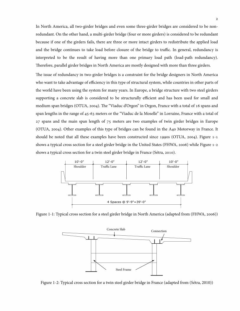
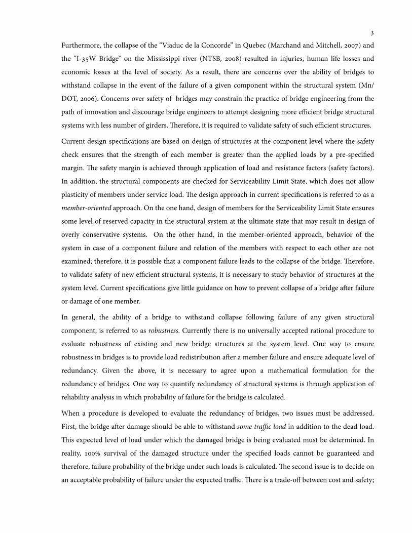
should be noted that all these examples have been constructed since s (OTUA, ). Figure -
shows a typical cross section for a steel girder bridge in the United States (FHWA, ) while Figure -
shows a typical cross section for a twin steel girder bridge in France (Sétra, ).
Figure 1-1: Typical cross section for a steel girder bridge in North America (adapted from (FHWA, ))
Figure 1-2: Typical cross section for a twin steel girder bridge in France (adapted from (Sétra, 2010))
10'-0" 12'-0" 12'-0" 10'-0"
4 Spaces @ 9'-9"=39'-0"
Shoulder ShoulderTra!c Lane Tra!c Lane
Concrete Slab Connection
Steel Frame
Furthermore, the collapse of the “Viaduc de la Concorde” in Quebec (Marchand and Mitchell, ) and
the “I-W Bridge” on the Mississippi river (NTSB, ) resulted in injuries, human life losses and
economic losses at the level of society. As a result, there are concerns over the ability of bridges to
withstand collapse in the event of the failure of a given component within the structural system (Mn/
DOT, ). Concerns over safety of bridges may constrain the practice of bridge engineering from the
path of innovation and discourage bridge engineers to attempt designing more efficient bridge structural
systems with less number of girders. erefore, it is required to validate safety of such efficient structures.
Current design speci'cations are based on design of structures at the component level where the safety
check ensures that the strength of each member is greater than the applied loads by a pre-speci'ed
margin. e safety margin is achieved through application of load and resistance factors (safety factors).
In addition, the structural components are checked for Serviceability Limit State, which does not allow
plasticity of members under service load. e design approach in current speci'cations is referred to as a
member-oriented approach. On the one hand, design of members for the Serviceability Limit State ensures
some level of reserved capacity in the structural system at the ultimate state that may result in design of
overly conservative systems. On the other hand, in the member-oriented approach, behavior of the
system in case of a component failure and relation of the members with respect to each other are not
examined; therefore, it is possible that a component failure leads to the collapse of the bridge. erefore,
to validate safety of new efficient structural systems, it is necessary to study behavior of structures at the
system level. Current speci'cations give little guidance on how to prevent collapse of a bridge aer failure
or damage of one member.
In general, the ability of a bridge to withstand collapse following failure of any given structural
component, is referred to as robustness. Currently there is no universally accepted rational procedure to
evaluate robustness of existing and new bridge structures at the system level. One way to ensure
robustness in bridges is to provide load redistribution aer a member failure and ensure adequate level of
redundancy. Given the above, it is necessary to agree upon a mathematical formulation for the
redundancy of bridges. One way to quantify redundancy of structural systems is through application of
reliability analysis in which probability of failure for the bridge is calculated.
When a procedure is developed to evaluate the redundancy of bridges, two issues must be addressed.
First, the bridge aer damage should be able to withstand some traffic load in addition to the dead load.
is expected level of load under which the damaged bridge is being evaluated must be determined. In
reality, survival of the damaged structure under the speci'ed loads cannot be guaranteed and
therefore, failure probability of the bridge under such loads is calculated. e second issue is to decide on
an acceptable probability of failure under the expected traffic. ere is a trade-off between cost and safety;

higher safety implies an increase in cost while risk of failure should be de'ned for the bene't of public.
erefore, an optimum failure probability should be agreed upon while it can be argued that this decision
is not just a matter of engineers but the society as well.
1.2. Purpose and Objectives
e purpose of this thesis is to demonstrate that two-girder or two-web structural systems can be
employed to design bridges with efficient use of materials while ensuring safety and adequate level of
redundancy.
In order to ful'll the above purpose, a procedure is developed to evaluate redundancy of any given bridge
structure as part of the broader concept of robustness. Reliability analysis of structures is utilized to
quantify redundancy and as part of the procedure, behavior of structural systems aer damage to a
critical member is studied. Expected traffic loads for intact and damaged bridges are modeled and an
acceptable margin for probability of failure is determined.
e developed procedure is applied to determine redundancy of bridges with two-girder or two-web
structural systems and indicate that these bridges can be designed such that an acceptable level of safety is
obtained. First, a three-span twin steel girder bridge is selected as a conventional steel system. Although
two-girder bridges are currently classi'ed as non-redundant structures, the effect of load redistribution in
continuous multi-span structures is considered. Second, application of new materials such as high-
performance and ultra high-performance concrete permits designers to develop new bridge structures
with thin cross sections and less material. Recent studies at the University of Toronto have led to the
development of such high-performance systems (Li, ). e reliability of a concrete double-T girder
bridge with external unbonded tendons, developed at the University of Toronto, is evaluated.
Based on the above discussion, the two major objectives of this thesis are:
() To develop a working de'nition and mathematical formulation for the reliability analysis of
the bridges at the system level in probabilistic design. e developed procedure will be used to
assess redundancy level of intact and damaged bridges in case of an accident. As part of
developing the procedure, the expected traffic loads on intact and damaged bridges are
modeled and an acceptable level of failure probability for the structure is determined.
() To apply the proposed procedure on two distinct structural systems:
a. ree-span twin steel girder bridge
b. Concrete double-T girder bridge with external unbonded tendons

1.3. Background
In this section, the available knowledge on evaluation of bridges with regard to safety in both stages of
design and analysis is reviewed. In Section .., available speci'cations on the issue of redundancy at the
system level in common design codes are provided. In Section .., current state of the art research on
the subject is summarized.
1.3.1. Design Speci'cations
e AASHTO Load and Resistance Factor Design (LRFD) speci'cations suggest including
redundancy in the design process by introducing load factor modi"ers (AASHTO, ). e load factor
modi'ers are based on the “level of redundancy,” “operational importance” of the structure and the “level
of ductility.” Members are classi'ed as redundant or non-redundant based on their contribution to the
bridge safety. If failure of a member causes collapse, it is designated as non-redundant while collapse is
de'ned as “a major change in the geometry of the bridge rendering it un't for use.” Also, similar to
requirements for earthquake design, “operational importance” classi'es the bridge based on
consequences of the structure not being in service. Finally, designers have to make a decision on the
classi'cation of ductility level for a member. Each of these three aspects is assigned a factor of ., . or
. depending on the classi'cation. A high level of redundancy, low level of operational importance and
high level of ductility are represented with a value less than .. A total load factor modi'er is obtained by
the product of the three factors (AASHTO, ). Although the above procedure considers the relation of
a member to the overall system, the main focus is nevertheless at the component level and it does not
address the question of acceptable behavior of a bridge aer damage or failure of a member. Also, current
literature suggests that, at some points, determination of load factor modi'ers become subjective. For
example, no clear guideline is provided for classi'cation of member ductility and the decision is le to
the designer (Ghosn and Moses, ). As a result, Ghosn and Moses () state that the procedure
requires further re'nement .
e AASHTO speci'cations for the design of highway bridges brie1y de'nes a non-redundant
structure as one in which “failure of a single element could cause collapse.” e speci'cations do not
provide more detailed background on this concept and only require that redundancy to be taken into
account when designing steel bridge members. e proper loading to evaluate a damaged structure aer a
component failure is not speci'ed. (AASHTO, )

e Canadian Highway Bridge Design Code (CHBDC) de'nes single-load-path and multiple-load-
path structures (CSA, a). A structure in which the failure of any primary component or connection
will cause the structure to collapse is classi'ed as a single-load-path, while a multiple-load-path structure
is de'ned as a system of components in which the failure of any primary component or connection will
not cause the structure to collapse. is standard speci'es that engineers should identify critical
components in single-load-path structures and ensure that they will not fail. e CHBDC classi'es
bridges with two-girder systems or a single steel box girder with two webs as single-load-path structures
and notes that these types of structures preferably should not be used. In Section . of the code,
fracture-critical members in steel structures are de'ned as members or portions of members in single-
load-path structures that are subject to tensile stress and the failure of which can lead to collapse of the
structure. e CHBDC requires increased level of material toughness to enhance safety and the engineer
is required to identify and take extra care in the design of such members. Overall, the code states that
evaluation of bridges at the system level depends on the will of the owner. (CSA, a) e CHBDC
does not provide a systematic procedure to evaluate redundancy of bridges at the system level and only
provides general statements about the issue.
e Eurocode Standards were expected to be fully implemented in European countries by to replace
national codes. e 'nal dra of “Eurocode : Actions on Structures - Part -: Accidental Actions” was
approved by the European Committee for Standardization (CEN) in (Gulvanessian and
Vrouwenvelder, ). Accidental action is de'ned as “an action, usually of short duration but of
signi'cant magnitude that is unlikely to occur on a given structure during the design working life.” Fire,
explosion, impact and earthquake are examples of accidental actions that can be identi"ed by the
designer, while human error, terrorist attack and exposure to aggressive agencies are harder to identify.
is standard also classi'es structures based on consequences of their failure (CEN, ). Aer
classifying the type of accidental action and the structure, the speci'cations require the designer to either
employ provisions to prevent the hazard, design to sustain the hazard or provide alternate load paths. is
standard recognizes that a zero risk level can never be achieved and that consequences of an accidental
action should be evaluated considering perceived public reaction and economy of safety provisions . e
standard states that risk analysis involves extensive statistical analysis and except for special cases,
qualitative risk analysis and “envisaged counter measures” should be adequate (CEN, ). e
guidelines are not speci'c to bridges and either provide speci'c guidelines for particular actions or
require counter measures to avoid collapse.

1.3.2. Analytical Level
is section reviews current state of research on concepts of robustness and redundancy.
e nature of events such as explosions, accidents or 're that may cause a structure to fail is random and
the behavior of structures in such events are also hard to predict. As a result, it is expected that concepts
of probability are utilized to quantify acceptable behavior of structures in case of an extreme event. Given
the above explanation, there are two problems with many of current available publications. First, current
publications, (Ressler, ), (Vrouwenvelder, ) or (Agarwal et al., ), employ detailed theoretical
stochastic modeling concepts that are hard to implement in practice and second, the proposed procedures
are developed for analysis of a particular structure or a speci'c accidental event such as ship collision in
offshore bridge structures (IABSE, ) or robustness of frame structures (Val and Val, ).
Furthermore, results of research in the area of structural safety have led to publication of two distinct sets
of guidelines. e 'rst document is published by the United States National Cooperative Highway
Research Program (NCHRP) (Ghosn and Moses, ) and the second document is published by the
Joint Committee on Structural Safety (JCSS) (JCSS, ), recognized mainly in Europe. e two
documents are explained below.
As stated previously, one way to ensure robustness is to provide redundancy in the structural system.
Currently, the United States National Cooperative Highway Research Program (NCHRP) Report No.
provides a set of guidelines to determine redundancy of bridges at the system level (Ghosn and Moses,
). e report provides a mathematical formulation of the safety index for a bridge structural system
and introduces System Factors that are used to evaluate redundancy level of a bridge. ese factors are
based on the performance of existing redundant bridges and work similar to load factors in current
design speci'cations, where resistance of a system must be checked against applied loads magni'ed by
system factors. e objective of the report was to ensure a minimum safety level for intact bridges and
damaged structures. In the NCHRP Report No. , Ghosn and Moses () employed system factors,
organized in tables, to provide a simple tool to evaluate safety of bridges, but the available tables are only
applicable to bridges with parallel members of equal capacity. Individual tables are provided for simple-
span or continuous steel and pre-stressed concrete multi-girder bridges. Although the procedure seems to
be the most complete study on redundancy of bridges at the system level, the guidelines are applicable
only to bridges with two lanes of traffic and conservative assumptions are made for the applied expected
traffic loads on damaged bridges.
In , the Joint Committee on Structural Safety (JCSS) published a document containing a set of new
guidelines for robustness evaluation of structural systems titled “Risk Assessment in Engineering -
Principles, System Representation & Risk Criteria.” e document includes an Annex on the “Assessment
of Structural Robustness.” Robustness is considered to be a broad concept and evaluation of an existing or
a new structural system with regard to robustness involves various aspects such as probability of failure,
acceptable extent of an initial local failure, acceptable extent of collapse progression and acceptable extent
of damage to the remaining structure in case of an initial failure. In order to quantify robustness a
framework for risk-based decision making is developed and direct or indirect effects of a component
failure are considered. In the procedure, following a “damage event,” direct and indirect consequences of
the event are calculated based on the vulnerability of the system and robustness is de'ned as a ratio
between direct risks and the total risks (JCSS, ). e document is intended for any structural system
and is not speci'c to bridges, which results in approaching the issue at the theoretical level. e document
is mainly focused on probabilistic aspects of a given 1aw in a system and although logical, it does not
provide a practical mathematical characterization for the concept of robustness in bridges.
1.3.3. Summary
Overall, at the design stage, available speci'cations identify the concept of redundancy and state the
importance of its application but fail to provide a comprehensive guideline to quantify redundancy for a
bridge. At the analytical level, in current literature, it is realized that consequences of failure can be severe
and involve risk of injury or life, inconveniences and losses incurred at the level of society. It is also
recognized that there is a need to de'ne a proper procedure to quantify safety of any structural system.
ere have been attempts to address the issue but the proposed procedures are mostly theoretical and fail
to 'll the gap between the member-oriented approach in current design standards and behavior of
structures at the system level.
All of the above described guidelines address the issue of redundancy in structural systems using a
probabilistic approach to account for uncertainties in performance of the components in a bridge. For the
purpose of this thesis, available guidelines in the NCHRP Report No. will be used and modi'ed to
employ the probabilistic approach of reliability analysis in order to calculate redundancy of bridges at the
system level. e procedure can also be used at the design stage for bridge structural systems. Quantifying
complete range of potential loadings on structures and associated probabilities of occurrence for those
load scenarios are part of the proposed method.

1.4. esis Outline
Based on the de'ned objectives and limitations of current available literature, several research tasks will
be completed in a sequential order. is thesis is organized in eight chapters to address the tasks related to
the objectives of this work as follows:
Chapter provides a general overview of the work and de'nes objectives of this thesis.
Chapter provides the necessary background knowledge on reliability analysis. e concept of reliability
analysis in bridges and conventional safety factor calculations for structural members are introduced. A
procedure is then developed to calculate the safety index and evaluate reliability of intact and damaged
bridges at the system level.
Chapter de'nes a relevant load model for the reliability evaluation of bridges at the system level. Dead
and live load parameters for bridges with two and three lanes of traffic are provided. Values of expected
maximum truck loads for various exposure times, probability density function for different transverse
truck positions and probability of various loading cases are de'ned. In addition, possible damage
detection intervals for a bridge with a failed member is discussed.
Chapter provides a discussion on the acceptable probability of failure for bridges at the system level. It
identi'es the level of load that a damaged bridge should be able to withstand before closure to traffic. It
outlines and compares the available guidelines on limiting values of the failure probability.
Chapter summarizes the procedure developed in Chapters , and as a set of guidelines. It also
provides two 1owcharts to demonstrate step-by-step approach to evaluate redundancy of bridges at the
system level.
Chapter applies system reliability guidelines from Chapter to a bridge concept with twin steel girders
and a composite concrete deck. Nonlinear structural analysis of the bridge at ultimate state is explained.
System safety indices for the bridge at intact and damaged conditions are calculated and it is
demonstrated that two-girder bridge structural systems can have sufficient degree of redundancy.
Chapter applies the developed system reliability guidelines to a bridge concept with a double-T concrete
girder and external unbonded tendons. Nonlinear structural analysis of the bridge at ultimate state is
explained. System safety indices for the intact and damaged bridge are calculated and it is demonstrated
that this type of structural system has the potential to be incorporated in the design of redundant systems.
Chapter concludes the thesis. It highlights contributions and achievements of this research and
suggestions for future work are discussed.

Common statistical de'nitions utilized to derive safety factor formulation or used through out this thesis
are provided in Appendix A.
1.5. De'nitions
A set of de'nitions for terms pertinent to this research is provided:
Robustness: is de'ned as the ability to withstand collapse following failure of any given structural
component.
Bridge Redundancy: is de'ned as the ability of a bridge to redistribute the applied load aer one of
the main load carrying components reaches its ultimate capacity or gets damaged.
Probabilistic Approach: is a method applicable to a system with inherent randomness where for a
given initial condition, the outcome varies but can be predicted (Haldar and Mahadevan, ).
Deterministic Approach: is a method applicable to a system with no randomness where for a given
initial condition, the outcome is always the same (Haldar and Mahadevan, ).
Collapse mechanism: A collapse mechanism is formed when a structure experiences high levels of
deformation and is no longer stable.
Collapse: is de'ned as the state at which collapse mechanism forms or when the structure
undergoes high level of damage.
Progressive Collapse: occurs when failure of a component in a system extends to the failure of
nearby components and eventually the overall system (Starossek, ).
Chapter 2
Reliability Analysis of Bridges at the System Level
e purpose of this chapter is to develop a formulation for reliability analysis of a bridge at the system
level. e procedure is based on the guidelines provided in the NCHRP Report No. (Ghosn and
Moses, ) and relies on the available knowledge about reliability analysis of structural components.
e procedure incorporates lognormal formulation of the safety factor of a component to calculate
system-level safety index for a bridge at intact and damaged conditions. is procedure is developed for
the purpose of this thesis and will be later used to evaluate redundancy of two-girder and two-web
structural systems. is chapter begins with a background on the concept of reliability analysis and will
address the following subjects:
() eory of structural reliability
() Concept of safety factor
(a) Safety factor at the component level with normal variables
(b) Safety factor at the component level with lognormal variables
() Safety Index for a bridge at the system level based on the NCHRP Report No. guidelines
() Redundancy in bridge structural systems
2.1. Basic Concepts in Reliability eory
2.1.1. Structural Reliability
Planning and design of most engineering projects is achieved by making sure that supply at least satis'es
the demand (Haldar and Mahadevan, ). In the 'eld of structural engineering demand can be
expressed as the applied load or a combination of loads, while supply is indicated by the strength,
resistance or capacity of a member or a system as a whole.
Supply, demand and their related parameters are frequently random quantities. Considering uncertainties
in the process of planning, design and construction of a structural system, perfect performance of a
system cannot be expected or achieved; alternatively if certain criteria are taken into consideration, a
satisfactory performance can be quanti'ed by the probability of success. is probabilistic assurance of
the performance has been de'ned as reliability. (Haldar and Mahadevan, )
Reliability analysis deals with uncertainties in a system that come from different sources. Statistical
uncertainties and modeling uncertainties can be classi'ed as quantitative factors. Quality, skill and
experience of construction workers, engineers and environmental impacts are hard to measure and can
be classi'ed as qualitative factors. erefore, it is important to develop appropriate design procedures to
incorporate risks associated to these uncertainties and satisfy a degree of safety.
In structural engineering practice, it is common for engineers to rely on certain standards and
speci'cations, such as the Canadian Highway Bridge Design Code (CHBDC) to achieve a successful and
safe design. is is due to the fact that realistic analysis of a structural system can be a signi'cant task
even at a deterministic level, thus certain idealizations and simpli'cations are made for the purpose of
system analysis. Simpli'cations at the design or evaluation stage of a structure can be classi'ed into three
categories: load modeling (applied load and load sequence), system modeling (structural system and its
components) and material modeling (material response and its strength): (Melchers, )
. Load Modeling: Realistically, it is possible that some parts of the structure reach failure point due to an
applied load sequence over time, while sequence of the applied load is a random process. Due to this
randomness, it is not an easy task to analyze the structure under various load sequences. erefore,
components of a system are generally analyzed under time independent load models and the design is
checked for an extremely uncertain load. (Melchers, )
. System Modeling: In system modeling, primary load-carrying components of structural systems are
modeled while potential mechanical behavior of secondary elements, such as barriers, sidewalks,
diaphragms etc.), are generally ignored to reduce complexity of the analysis. In addition, modeling
nonlinear performance of structural systems and interaction of the components with each other are not
easy and simplifying assumptions should generally be made. Simpli'cations such as reducing the scope
from a realistic three- dimensional analysis to a more practical two-dimensional analysis are oen
employed in the design and evaluation of structures.
. Material Modeling: It is hard to accurately predict nonlinear behavior of materials, de'ne transition
points from elastic to plastic phases and determine the mechanical properties of materials at various
phases. Different strength-deformation relationships such as elastic, elastic-brittle and elastic-plastic are
generally used to model mechanical behavior of materials. (Melchers, )
Given all the uncertainties in modeling of the applied loads, the structural system and the behavior of
materials, absolute success in the performance of structural systems cannot be guaranteed. If different
samples of a structural element with the same nominal size and the same material composition are tested
in a laboratory, under controlled conditions and under the same applied load, resistance of the material
will vary between the samples. is implies that resistance of the samples is not deterministic. With the
same reasoning, strength of materials used in practice may be less than what is incorporated in the
calculations or applied loads may be greater than what has been originally anticipated.
Current design speci'cations employ safety factors to account for uncertainties in the design and
evaluation of structures and prevent local failure of components in the system. Determination of a safety
factor is based on the failure probability of members that incorporates the uncertainties in applied loads
and resistance of the structural components. However, a decision has to be made on a target failure
probability that ensures acceptable performance of the structure. When de'ning the target failure
probability, it is considered that consequences of failure and extent of damage can be severe. In addition,
failure of a system or an element of a structure greatly affects replacement cost of the failed structure.
Loss of life or injuries incurred as a result of failure or cost associated to the loss of time for the society are
among other reasons that determines the acceptable failure probability and as a result the safety factors.
(MacGregor, )
2.1.2. Safety Factor Concept
e concept of safety factor has been used in both deterministic and probabilistic designs. In
deterministic design the value of safety factor is based on past experience and intuition. Sensitivity of
components made of a particular material under a special loading condition can be studied in practice,
and a safety factor can be established based on uncertainties experienced. In the deterministic approach,
it is assumed that the structure survives as long as the nominal value of load does not exceed the nominal
load carrying capacity of the structure. In other words, the ratio of applied loads to member resistance
should always be less than one. e probabilistic design approach calculates a similar safety factor but
provides a methodology to establish reliability of an element based on the probability of failure in which a
margin of safety is considered. e background on the safety factor calculation in both deterministic and
probabilistic approaches are further reviewed in the following paragraphs.
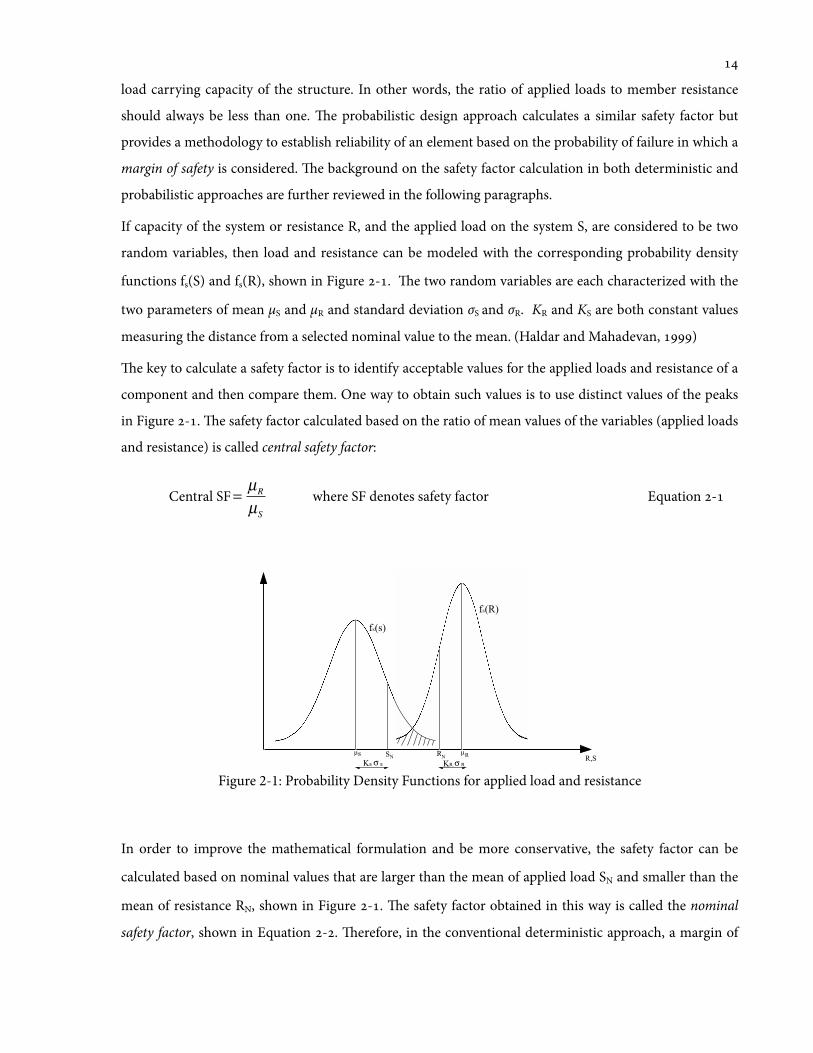
If capacity of the system or resistance R, and the applied load on the system S, are considered to be two
random variables, then load and resistance can be modeled with the corresponding probability density
functions fs(S) and fs(R), shown in Figure -. e two random variables are each characterized with the
two parameters of mean μS and μR and standard deviation σS and σR. KR and KS are both constant values
measuring the distance from a selected nominal value to the mean. (Haldar and Mahadevan, )
e key to calculate a safety factor is to identify acceptable values for the applied loads and resistance of a
component and then compare them. One way to obtain such values is to use distinct values of the peaks
in Figure -. e safety factor calculated based on the ratio of mean values of the variables (applied loads
and resistance) is called central safety factor:
Central SF=µR
µS
where SF denotes safety factor Equation -
Figure 2-1: Probability Density Functions for applied load and resistance
In order to improve the mathematical formulation and be more conservative, the safety factor can be
calculated based on nominal values that are larger than the mean of applied load SN and smaller than the
mean of resistance RN, shown in Figure -. e safety factor obtained in this way is called the nominal
safety factor, shown in Equation -. erefore, in the conventional deterministic approach, a margin of
fs(s)
!!s RS RN N R,S
Ks"s KR"R
fs(R)

safety is achieved through selection of two absolute but conservative values of load and resistance RN and
SN. (Haldar and Mahadevan, )
Nominal SF = RN
SN= KR
KS
(Central SF) Equation -
In the above deterministic approach, the safety factor is calculated unrealistically based on the absolute
limits of two uncertain quantities. is method has been helpful in designing structures for a long time,
although for different structures the probability of failure would not be the same for the same applied
factor of safety. e level of uncertainty in applied loads or member resistance differs for various types of
loads, materials or structural systems. erefore, the above formulation of safety factor may introduce a
satisfactory conservatism in design of structures, yet it does not realistically represent the actual margin
of safety for a member. (Haldar and Mahadevan, )
e above concept can be further extended using the overlapped area (shaded region) between the two
curves R and S in Figure -. is is an area where resistance is less than the applied loads and it
represents a quantitative measure for the probability of failure. is probability of failure depends on the
following three factors: (Haldar and Mahadevan, )
. If the shaded area decreases, probability of failure also decreases. For this to happen, the two
curves should move away from each other.
. Based on the standard deviation of the two curves, dispersion of the curves may vary
signi'cantly. If there is little dispersion, curves will be narrow and the overlapped area gets
smaller leading to a smaller probability of failure for the structure.
. Finally shape of the curves are affected by probability density functions fs(S) and fs(R), leading to
smaller or greater overlapped area and therefore, smaller or greater probability of failure.
e overlapped area between the two curves can be controlled by selection of the two design variables,
namely load and resistance. ese variables can be selected such that the area is minimized and a safe
design is achieved. In the conventional approach, application of safety factor shis the two curves away
from each other and sets design variables such that the required safety is obtained. In a more accurate and
advanced method all the above three factors affecting position of the two curves and the actual risk of
failure are considered. In other words, design variables are de'ned such that an acceptable level of risk is
achieved. is way unsatisfactory performance or behavior against certain performance criteria in design
and reliability of the system are taken into consideration. is is the foundation of risk-based design
concept. (Haldar and Mahadevan, )
2.1.3. Conventional Safety Factor - Single Load Case with Normal Variables
In this section, the conventional method to calculate safety factor for a member in a probabilistic based
design is reviewed. is will be the basis for calculation of safety index at the system level.
e case of only one applied load S (dead load, live load, wind load, etc.) on a component with the
resistance R is considered. All formulas and equations in Sections .. and .. are according to Haldar
and Mahadevan (). It is assumed that both R and S are normal variables with N(μR,σR) and N(μS,σS)
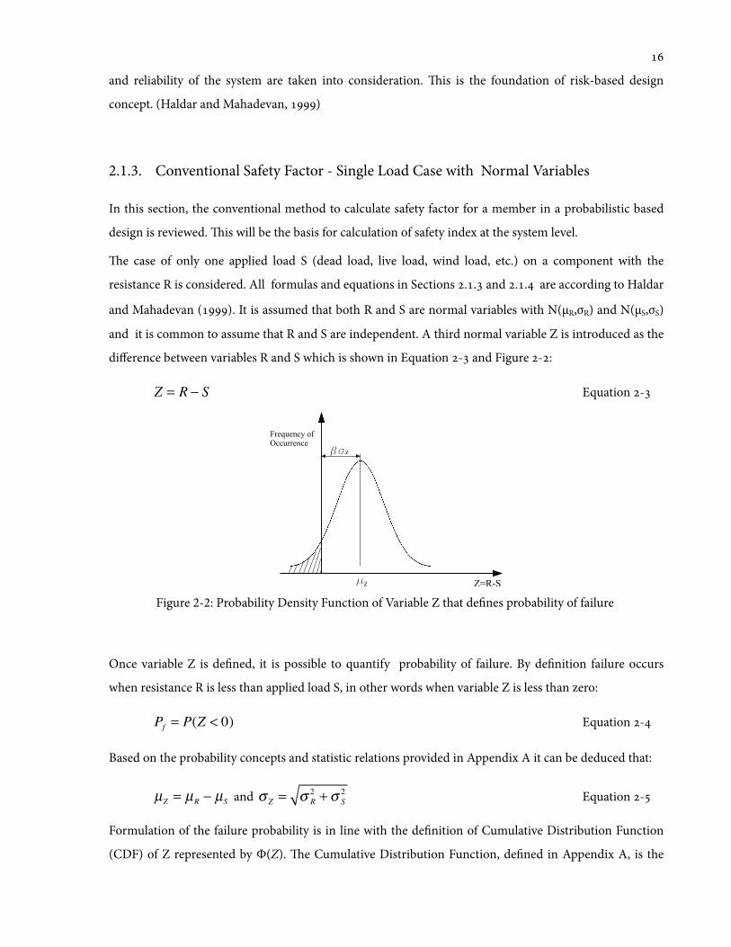
and it is common to assume that R and S are independent. A third normal variable Z is introduced as the
difference between variables R and S which is shown in Equation - and Figure -:
Z = R − S Equation -
Figure 2-2: Probability Density Function of Variable Z that de'nes probability of failure
Once variable Z is de'ned, it is possible to quantify probability of failure. By de'nition failure occurs
when resistance R is less than applied load S, in other words when variable Z is less than zero:
Pf = P(Z < 0) Equation -
Based on the probability concepts and statistic relations provided in Appendix A it can be deduced that:
µZ = µR − µS and σ Z = σ 2R +σ
2S Equation -
Formulation of the failure probability is in line with the de'nition of Cumulative Distribution Function
(CDF) of Z represented by Φ(Ζ). e Cumulative Distribution Function, de'ned in Appendix A, is the
!"!
#" "#$%&
'()*+),-./01/2--+((),-)
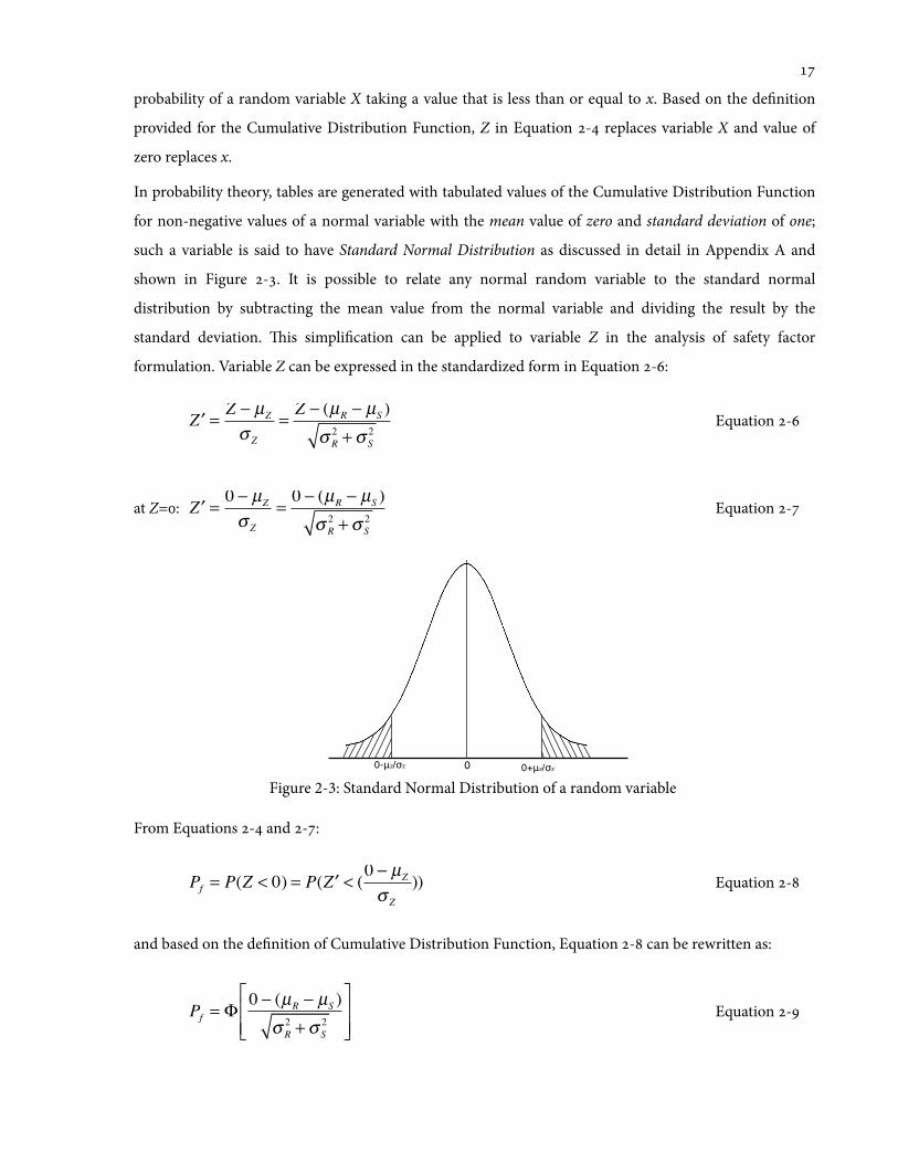
probability of a random variable X taking a value that is less than or equal to x. Based on the de'nition
provided for the Cumulative Distribution Function, Z in Equation - replaces variable X and value of
zero replaces x.
In probability theory, tables are generated with tabulated values of the Cumulative Distribution Function
for non-negative values of a normal variable with the mean value of zero and standard deviation of one;
such a variable is said to have Standard Normal Distribution as discussed in detail in Appendix A and
shown in Figure -. It is possible to relate any normal random variable to the standard normal
distribution by subtracting the mean value from the normal variable and dividing the result by the
standard deviation. is simpli'cation can be applied to variable Z in the analysis of safety factor
formulation. Variable Z can be expressed in the standardized form in Equation -:
′Z =Z − µZ
σ Z
=Z − (µR − µS )
σ R2 +σ S
2Equation -
at Z=: ′Z =0 − µZ
σ Z
=0 − (µR − µS )
σ R2 +σ S
2Equation -
Figure 2-3: Standard Normal Distribution of a random variable
From Equations - and -:
Pf = P(Z < 0) = P( ′Z < (0 − µZ
σ Z
)) Equation -
and based on the de'nition of Cumulative Distribution Function, Equation - can be rewritten as:
Pf = Φ0 − (µR − µS )
σ R2 +σ S
2
⎡
⎣⎢⎢
⎤
⎦⎥⎥
Equation -
00-!z/"z 0+!z/"z
Due to symmetry in Figure -, the area under the positive and negative sides of the curve, which are set
by equal distances from the origin, are equal. By de'nition the probability that an event does not occur is
equal to minus the probability that it does occur. Application of the above axioms to Equations - and
- results in Equation -:
P( ′Z < (0 − µZ
σ Z
)) = P( ′Z > (0 + µZ
σ Z
)) = 1− P( ′Z < (0 + µZ
σ Z
))
Pf = 1− Φ(µR − µS )σ R2 +σ S
2
⎡
⎣⎢⎢
⎤
⎦⎥⎥
Equation -
where Φ is the Cumulative Distribution Function of a standard normal variable. Finally when Equation
- is rearranged, the safety index formulation can be derived as:
µR = µS +Φ−1(1− Pf ) σ R2 +σ S
2 Equation -
e value of Φ1(-Pf), in Equation -, represents inverse of the standard normal variable
corresponding to the probability level (-Pf). Let β=Φ1(-Pf); therefore:
β = Φ−1(1− Pf ) =(µR − µS )σ R2 +σ S
2Equation -
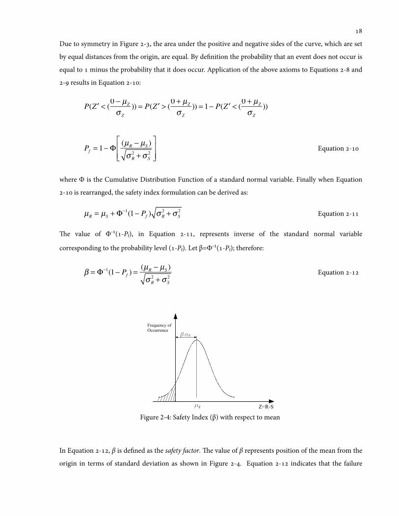
Figure 2-4: Safety Index (β) with respect to mean
In Equation -, β is de'ned as the safety factor. e value of β represents position of the mean from the
origin in terms of standard deviation as shown in Figure -. Equation - indicates that the failure
!"!
#" "#$%&
'()*+),-./01/2--+((),-)
probability of structures is directly related to the mean and standard deviation of loads and resistance. In
this formulation safety index is related to the probability of failure and if β increases Pf decreases resulting
in a smaller risk of failure. (Haldar and Mahadevan, )
2.1.4. Conventional Safety Factor- Single Load Case with Lognormal Variables
A safety factor deals only with the mean and standard deviation values of variables and it is not necessary
to determine detailed form of variable distributions. In reliability analysis load and resistance are
generally modeled with normal or lognormal distributions, although the actual physical patterns may not
entirely follow these distributions. e main difference between the two distributions is that lognormal
variables cannot take negative values. Load and resistance are also positive quantities due to their physical
properties; therefore, it is logical to model these variables with lognormal distribution. (Haldar and
Mahadevan, ) In this section the procedure to formulate safety index with lognormal variables is
explained:
For this purpose, it is assumed that R and S are lognormal variables and a new random variable Y is
introduced where normal variable Z can be de'ned as the natural logarithm of Y.
Y = R / S and Z = lnY = lnR − lnS Equation -
In Section .., probability of failure for normal variables was de'ned as Z, when the value of Z was less
than zero (Z<). Accordingly, based on Equation - probability of failure can be expressed as Y<..
e natural logarithm of a lognormal variable is normal; therefore, Z which is de'ned as the natural
logarithm of quotient of two independent lognormal variables is also a normal distribution, Equation
-. e parameters for normal distribution of Z is calculated similar to the principles stated for sum or
difference of two independent distributions in Appendix A.
Z ≈ N(λR − λS , ζR2 +ζS
2 ) Equation -
Probability of failure can now be expressed similar to the procedure described for normal variables in
Section ..:

Pf = 1− ΦλR − λSζR2 +ζS
2
⎛
⎝⎜
⎞
⎠⎟ Equation -
If the relationships between mean, standard deviation, coefficient of variation and parameters of
lognormal distributions provided in Appendix A are applied to the above equation, the following
equation can be derived:
Pf = 1− Φ
ln µR
µS
⎛⎝⎜
⎞⎠⎟⋅ 1+VS
2
1+VR2
⎧⎨⎪
⎩⎪
⎫⎬⎪
⎭⎪ln(1+VR
2 )(1+VS2 )
⎛
⎝
⎜⎜⎜⎜⎜
⎞
⎠
⎟⎟⎟⎟⎟
Equation -
In Equation -, VS and VR (coefficient of variation for load and resistance respectively) can be assumed
to be relatively small and negligible, e.g. less than .. Equation - is now simpli'ed and rewritten as:
Pf ≈ 1− Φln µR
µS
⎛⎝⎜
⎞⎠⎟
⎧⎨⎩⎪
⎫⎬⎭⎪
VR2 +VS
2
⎛
⎝
⎜⎜⎜⎜
⎞
⎠
⎟⎟⎟⎟
Equation -
Rearranging Equation - where β=Φ1(-Pf) and (-Pf) represents the inverse of cumulative
distribution function, the following is derived:
β ≈ln µR
µS
⎛⎝⎜
⎞⎠⎟
⎧⎨⎩⎪
⎫⎬⎭⎪
VR2 +VS
2Equation -
Based on the safety factor formulation presented in Sections .. and Equation -, a safety factor
accounts for uncertainties in estimating member resistance as well as the applied loads. e design load
and resistance factors provided in the Canadian Highway Bridge Design Code (CHBDC) or the
AASHTO LRFD Bridge Design Speci'cations are derived from calibration of member design checks to
arrive at a uniform value of β (Nowak and Szerszen, ). For example, the Ontario Highway Bridge
Design Code employed the available database of existing bridges assembled in in Ontario to arrive
at a member safety factor of ..
2.2. Safety Index for Bridges at the System Level
A safety factor can be used to measure reliability of structural components as well as structural systems.
Current design and evaluation techniques calculate the safety factor at the component level and generally
ignore behavior of the structural systems. is approach does not provide a true measure for safety of
bridges at the system level. In many cases, failure of an individual member due to extreme events not
foreseen in the design speci'cations such as 're, corrosion or collision with a vehicle does not necessarily
lead to the failure of a bridge. It is the designer's duty to make sure bridges can withstand accidental
damage and operate under anticipated traffic until closure. erefore, it is important to evaluate behavior
of structures aer failure of a critical component and determine the level of redundancy of structural
systems. Values of the system safety index for a bridge at intact and damaged conditions can be used to
quantify redundancy. e concept of safety factor at the component level, with a slight change, can be
adapted to calculate system-level safety index for a bridge at both intact and damaged conditions.
In order to calculate the conventional safety factor for a structural component, mean values of R and S in
Equation - are generally represented in terms of bending moment (kN.m) or shear (kN). Moment or
shear values due to applied loads at a certain location of the component is estimated and compared to the
moment or shear resistance at that location.
β = Φ−1(1− Pf ) =(µR − µS )σ R2 +σ S
2Equation -
is is a reasonable procedure to calculate the safety factor of structural members since resistance of
components are generally represented in terms of moment or shear values, but the same approach may
not be applicable to structural systems. e problem arises when resistance of a system is calculated. For
example, in a bridge with multiple steel girders and a composite concrete deck slab, each girder takes part
of the total applied load which results in different values of moment and shear in the girders. It can be
argued that total resistance of a multi-girder structure can be estimated by adding up the moment values
of all girders at a critical location such as mid-span. is solution may solve the problem for parallel
girder bridges but may not be applicable to all structural systems. e procedure to calculate system safety

index is intended to be a general guideline that can be applied to all types of bridges; therefore, an
alternative approach is adapted.
In this thesis, the proposed procedure to calculate safety index for bridges is based on the work of Ghosn
and Moses as explained in the National Cooperative Highway Research Program (NCHRP) Report No.
(Ghosn and Moses, ). e NCHRP guidelines are modi'ed to reduce complexities, generalize
the procedure and improve representing the actual bridge behavior under traffic. e guidelines and
applied modi'cations are discussed in this section.
Based on the NCHRP Report No. approach, resistance of a bridge can be represented in terms of the
total number of (standard) trucks that a bridge can withstand before collapse. Collapse is de'ned as the
state at which collapse mechanism forms or when the structure undergoes a high level of damage. A
collapse mechanism is formed when the structure experiences high levels of deformation and is no longer
stable. High levels of damage happens when critical members of the bridge lose their load carrying
capacity, e.g. crushing of concrete. e Load factor (multiplier of standard truck) that represents ultimate
resistance of an intact bridge at the system level is de'ned as LFu.
A bridge is assumed to be in a damaged state when one of its load carrying members loses capacity due to
an accident, fault in the member or etc. e ultimate capacity of damaged bridges can be represented by
the number of (standard) trucks that the bridge can withstand before collapse, LFd.
e NCHRP Report No. guidelines incorporate probabilistic characteristics of the reliability analysis
and employ LFu and LFd to derive intact and damaged system safety indices in which resistance of the
system is compared to the applied loads. Values of LFu and LFd can be determined through structural
analysis of the bridge, yet applied loads on the structure must be determined.
In addition to dead load, an intact bridge should be able to carry the maximum expected truck loads of its
design life time, generally years. e damaged bridge should withstand regular traffic in the exposure
period during which damage is expected to be detected and the bridge to be closed. Expected truck loads
come from the available statistical data on truck weights, position of trucks on the bridge deck, truck axle
con'guration and distribution of weight to individual truck axles. Details of the developed traffic load
model used in this study is presented in Chapter .
e expected maximum traffic loads for intact and damaged bridges can be represented as a factor of the
standard truck. is way applied load and system resistance, both expressed in terms of load factors, can
be incorporated in the safety index formula.
For the case of intact bridges, system resistance is represented by LFu and the applied maximum lifetime
live load by LF75. It is a common practice to assume that LFu and LF75 are random variables and follow

lognormal distribution. Based on the formulation of safety index in Sections .. and .., safety index
for an intact bridge at ultimate state can be expressed as follows:
βu =ln LFuLL75
VLF2 +VLL
2Equation -
where LFu is the mean value of the number of standard trucks that cause the bridge to collapse. is
value is the unfactored live load margin, Resistance less Dead load (R-D), indicating that LFu is related to
resistance of the system and dead load. LL75 is the mean value of the expected maximum lifetime live
load that includes dynamic load allowance effect. VLF is the coefficient of variation of LFu while VLL is the
coefficient of variation of LL75. Denominator of Equation - is a measure of uncertainties in estimating
resistance, dead load and expected maximum live load including dynamic impact. Values of mean,
standard deviation and coefficient of variation of applied loads will be discussed in Chapter . It remains
to calculate the coefficient of variation LFu.
Current available data to estimate coefficient of variation for resistance of bridges at the system level is not
sufficient but there have been substantial studies with proper statistical data on resistance of individual
bridge members. e reliability theory of structural systems indicates that coefficient of variation for a
system is generally smaller than that of its individual members (Ghosn and Moses, ). is is only
true when nonlinear structural analysis of the structure that is used to analyze and estimate capacity of
the system is exact. e NCHRP Report No. guidelines suggest that coefficient of variation of bridges
at system level be taken the same as the coefficient of variation of structural members to account for
uncertainties in nonlinear modeling of bridges. e statistical parameters of member resistance for
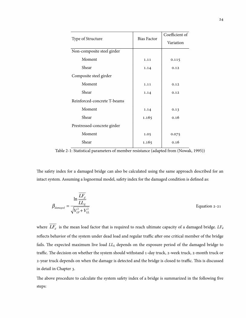
different types of structures are provided in Table -.
Type of Structure Bias FactorCoefficient of
Variation
Non-composite steel girder
Moment . .
Shear . .
Composite steel girder
Moment . .
Shear . .
Reinforced-concrete T-beams
Moment . .
Shear . .
Prestressed-concrete girder
Moment . .
Shear . .
Table 2-1: Statistical parameters of member resistance (adapted from (Nowak, 1995))
e safety index for a damaged bridge can also be calculated using the same approach described for an
intact system. Assuming a lognormal model, safety index for the damaged condition is de'ned as:
!damaged =
lnLFd
LLE
VLF2+VLL
2
! Equation -
where LFd is the mean load factor that is required to reach ultimate capacity of a damaged bridge. LFd
re1ects behavior of the system under dead load and regular traffic aer one critical member of the bridge
fails. e expected maximum live load LLE depends on the exposure period of the damaged bridge to
traffic. e decision on whether the system should withstand -day truck, -week truck, -month truck or
-year truck depends on when the damage is detected and the bridge is closed to traffic. is is discussed
in detail in Chapter .
e above procedure to calculate the system safety index of a bridge is summarized in the following 've
steps:

: Develop structural model of the bridge and perform nonlinear analysis of the structure,
incorporating the best estimate of material properties without reduction factors and apply the best
estimate of dead loads.
: Identify the most critical longitudinal position of standard trucks and consider multiple
transverse positions for the trucks. Do not include dynamic live load allowance factor.
: Apply truck loads to the structure and increase the load incrementally until ultimate limit state is
reached. Record load factor LFu.
: Identify a critical member of the structure such that failure in that member may cause serious
damage. Assume the member capacity is lost and keep loading the structure incrementally until it
fails. Calculate load factor LFd and repeat the procedure if there is more than one critical member.
Pick the lowest load factor, i.e. the most critical condition.
: Using LFu, LFd and the expected traffic on the bridge (explained in Chapter ) calculate the
system safety index for the intact and damaged bridge.
Now that a procedure to calculate the safety index for a bridge at the system level is developed,
redundancy of a bridge can be quanti'ed.
2.3. Redundancy in Bridges
In this section, 'rst the guidelines provided in the NCHRP Report No. to calculate redundancy is
summarized. en the proposed simpli'cation on the formulation, for the purpose of this thesis, is
provided.
e NCHRP Report No. guidelines calculate two more safety index values in addition to the system
safety indices at the intact and damaged conditions, namely: member safety index and functionality safety
index (Ghosn and Moses, ).
In the report a linear elastic analysis of the structural system is performed and a member safety index is
calculated. is index is based on the number of (standard) trucks that the bridge can withstand just
before the 'rst member reaches its ultimate capacity (LF) and provides a check for safety of all the
individual members.
e functionality safety index marks the stage at which the bridge is subject to large levels of permanent
deformation. De1ection limits are imposed to provide a measure for loss of functionality in the structural
system. According to the NCHRP guidelines, functionality safety index indicates the time at which the
bridge is no longer safe for the regular traffic, but it should be noted that the bridge does not necessarily
collapse at this stage.
Finally, safety indices for the intact and damaged bridges at the ultimate state are calculated. e level of
bridge redundancy is then de'ned as the difference between values of functionality, ultimate-intact and
ultimate-damaged safety indices with the member safety index. is results in a total of three relative
reliability indices. e level of redundancy is adequate when all three values satisfy the minimum
speci'ed limits provided in the report.
As previously described, redundancy is de'ned as the ability of a bridge to redistribute the applied load
aer one of its main load carrying components fails or is damaged. erefore, for the purpose of this
thesis, only the two ultimate system safety indices of the bridge at intact and damaged conditions are
employed to evaluate redundancy of a bridge at the system level. e reasons to exclude member or
functionality safety indices from the procedure are explained below.
e member safety index is not included as part of the proposed procedure because the index is more of a
design check than a redundancy check. According to the NCHRP Report No. , theoretically, member
safety index is only provided to check individual member safety based on current speci'cations and
elastic analysis. e guidelines state that the load modi'er LF can be calculated based on a linear elastic
structural model of the bridge. is check guarantees that bridge components are designed according to
the speci'cations. In the formulation of redundancy, the index is used as a datum to determine relative
index values while the acceptable limiting values of such relative indices are determined based on a
minimum member safety index of .. However, for the purpose of this research, it is assumed that the
bridge under study is already designed according to the code speci'cations and therefore, the values of
safety indices at ultimate can be used directly for the evaluation purposes.
In this thesis, when relevant, the load at which the bridge stops behaving linearly is calculated and called
LFlinear. e corresponding safety index can then be calculated as shown in Equation -. is safety
index is calculated for the twin steel girder bridge in Chapter . is is only to illustrate behavior of the
system at various loading stages and provide more insight into the range of safety index values, but it is
not included in determination of the redundancy of the bridge.
βlinear =ln LFlinLL75
VLF2 +VLL
2Equation -

e Functionality Safety Index is not taken into account because the goal of this thesis is to avoid sudden
collapse of the bridge and ensure safety under expected traffic loads. e bridge de1ections prohibited
under the functionality safety index can therefore be allowed as long as the bridge does not collapse. It
should be noted that certain de1ection limits are incorporated in the proposed procedure to determine
damage detection time and the expected traffic that the bridge should withstand before closure, this is
explained in detail in Chapter .
In summary, the objective is to ensure that the bridge can withstand expected traffic aer damage or
failure of a component; therefore, only safety index values at ultimate will be used for the intact and
damage bridge to evaluate the level of redundancy and reliability of the structural system.
Chapter 3
Bridge Load Models
In this chapter, applicable loads in the reliability analysis of bridges at the system level are modeled. e
load components considered in this study are dead load and live load including dynamic load allowance.
e expected traffic loads on both intact and damaged bridges are de'ned. Load models are based on the
available statistical data, surveys, inspection reports, and analytical simulations and are applicable to
bridges with two and three lanes of traffic. Load variation is described by cumulative distribution
function, mean value or bias factor (ratio of mean to nominal value) and coefficient of variation. is
chapter will address the following topics:
() Dead load model;
() Live load model for both intact and damaged bridge;
(a) Expected maximum load for various time intervals;
(b) Transverse position of trucks;
(c) Single and multiple lane loadings;
(d) Probability of occurrence for de'ned live load events;
() Expected loads in the formulation of the safety index.

3.1. Dead Load Model
Dead load is de'ned as the gravity load due to the weight of girders, deck slab, wearing surface, barriers,
sidewalks and diaphragms when applicable. e statistical parameters of dead load model are based on
existing bridges and the work of Nowak (). e weights of four components are considered in this
model as described below and shown in Table -:
. Factory made elements (steel and precast concrete members)
. Cast-in-place concrete members
. Wearing surface
. Miscellaneous items, (e.g. railings and luminaries)
Component Bias factor (mean/nominal) Coefficient of variation . . . . mm (mean thickness) . .-. .-.
Table 3-1: Statistical parameters for dead load model (adapted from Nowak, 1994)
In general, the best estimate of dead load should be used in the analysis of a bridge. One way to get a
reasonable estimate for dead load is to calculate weight of components based on the given dimensions on
bridge drawings and magnify them by the bias factor (mean/nominal) to account for the uncertainties in
construction of the component. is way the level of uncertainties experienced in construction of existing
bridges is incorporated in prediction of the expected dead load.
3.2. Live Load Model for Bridges with Two-Traffic Lanes
3.2.1. Expected Maximum Truck Weights
One of the most challenging aspects of bridge reliability analysis is the development of a live load model
that would represent traffic on a bridge. e reason is due to the large variability inherent in vehicle-
induced loads. (Ressler, ) Modeling the traffic load on a bridge involves more than specifying the
vehicle weight and includes many factors such as:
. Gross Vehicle Weight (GVW)

. Number of axles and their spacing
. Distribution of GVW on the axles
. Overall vehicle weight
. Multiple vehicle presence
. Transverse position of vehicles, and
. Characteristics of dynamic effect of live load
Live load is generally represented in the form of a design truck and it is assumed that the gross vehicle
weight (GVW) is a random variable. In this study, axle spacing and percentage of the total load per axle of
a truck remain constant. e CL- truck from the Canadian Highway Bridge Design Code (CHBDC) is
selected as the basis for the live load evaluation model. e CHBDC clause .. de'nes CL- truck
with 've axles at the given spacings shown in Figure -. Selection of this truck will automatically decide
values of the 'rst three parameters listed above. e remaining parameters will be discussed in the rest of
this section.
Figure 3-1: CL-625 truck load model (adapted from CSA, 2006a)
Truck weight distribution is adapted from the statistics used to calibrate the AASHTO LRFD live load
factors by Nowak (). Nowak’s parameters are based on the truck surveys originally conducted in
Ontario in . It should be noted that the survey included about , heavily loaded trucks and
although this is a relatively large number, it may not re1ect the actual number of heavy trucks for a -
year bridge life span. It was also expected that some very heavy trucks might have avoided the survey
purposefully. (Nowak, )
e Ontario truck weight data do not exactly 't a normal distribution, but Nowak assumed properties of
a normal variable for the truck weight dispersion and presented parameters of the population in terms of
the Ontario Highway Bridge Design (OHBD)- truck. Nowak’s report presents the cumulative
distribution of vehicle population in terms of bending moment for the simple span bridges shown in
Figure - (Nowak, ). e 'rst step to use Nowak's truck weight data is to convert the given
CL-625
25
125 125 175 15050
62.5 62.5 Wheel loads, kN
Axle loads, kN
3.6 m 1.2 m 6.6 m 6.6 m
7587.5

statistical parameters for the OHBD- truck in Nowak's study to equivalent parameters for the
CL- truck. In order to 'nd the mean value and standard deviation of truck population in terms of the
CL-, effect of the OHBD- truck is compared to that of the CL-.
Before the effect of two trucks are compared, the de'nition of the Standard Normal Distribution must be
reviewed. is concept will be used in the calculation of statistical parameters of the truck weight data. A
normal random variable with a probability density function having a mean of zero and variance of one is
said to have a Standard Normal Distribution. ere are tables which provide values of the cumulative
distribution function for a wide range of nonnegative values of a standard normal variable. ese tables
can be used to relate probability levels to the number of standard deviations (i.e. fractiles) that a
particular given value falls above the mean value (Moses, ). e concept is explained in detail in
Appendix A and the Standard Normal Distribution table is provided in Appendix B.
Figure 3-2: Cumulative distribution functions of truck moments from 1975 survey in terms of
OHBDC-1983 moment (Nowak, 1994)
e OHBD- truck creates a bending moment of kN.m for a -meter span while the CL-
truck creates a bending moment of kN.m for the same span. In Figure -, value of zero for the
Inverse Standard Normal Distribution Function represents the mean of the population. In this 'gure,
moment values are represented as a ratio of the OHBD truck with the corresponding mean of ..

erefore, Nowak's calibration leads to a mean maximum moment of .x=kN.m for the
OHBD- truck and -meter bridge span. e CL- truck should produce the same mean value for
the population. Similarly, the CL- truck will produce a mean maximum moment of W/ multiplied
by where W is mean of the population weight, when the CL- is the reference truck. erefore, it
only remains to 'nd W. is is shown below.
Nowak's approach for modeling traffic data is further explained and it will be used to calculate the
standard deviation of population.
e expected or mean maximum load depends on the number of loading events. at is, for a longer
duration the truck volume increases and consequently the maximum single truck-loading event
increases. Nowak used extreme events to estimate expected maximum truck loading in any given time
interval (Nowak, ). According to his methodology, the expected maximum value “closely
corresponds to an individual truck weight fractile corresponding to /N” where N is the number of load
events in a given exposure time. e truck weight fractile relates probability level to the number of
standard deviations that a given probability is above the mean value. e total number of truck-passings
for every time interval is used to calculate the event probability level. Number of truck loading events for
different exposure times are provided in Nowak’s report. Also, the Standard Normal Distribution Table is
used to 'nd the inverse normal (number of standard deviations) that should be added to the mean of the
population. is way, expected maximum single truck loading events for different exposure times ( day,
weeks, month, and etc. shown in Figure -) are obtained.
In summary, for a given time interval with N truck loading events:
Mean maximum truck = Mean of population + Standard deviation × Normal variate for /N level
CL-625 Truck (CL 3.8.3.2, CHBDC) and OHBDC-1983 Truckto !nd the mean:
27 m long span2881 kN.m moment of the OHBD-1983 truck625 kN standard vehicle weight, CL-625 truck
2510 kN.m moment of the CL-625 truck 0.48 mean maximum moment for a simple span due to a single truck
(From Nowak CDF)
344 mean of the population (W) in terms of the CL-625 truck load
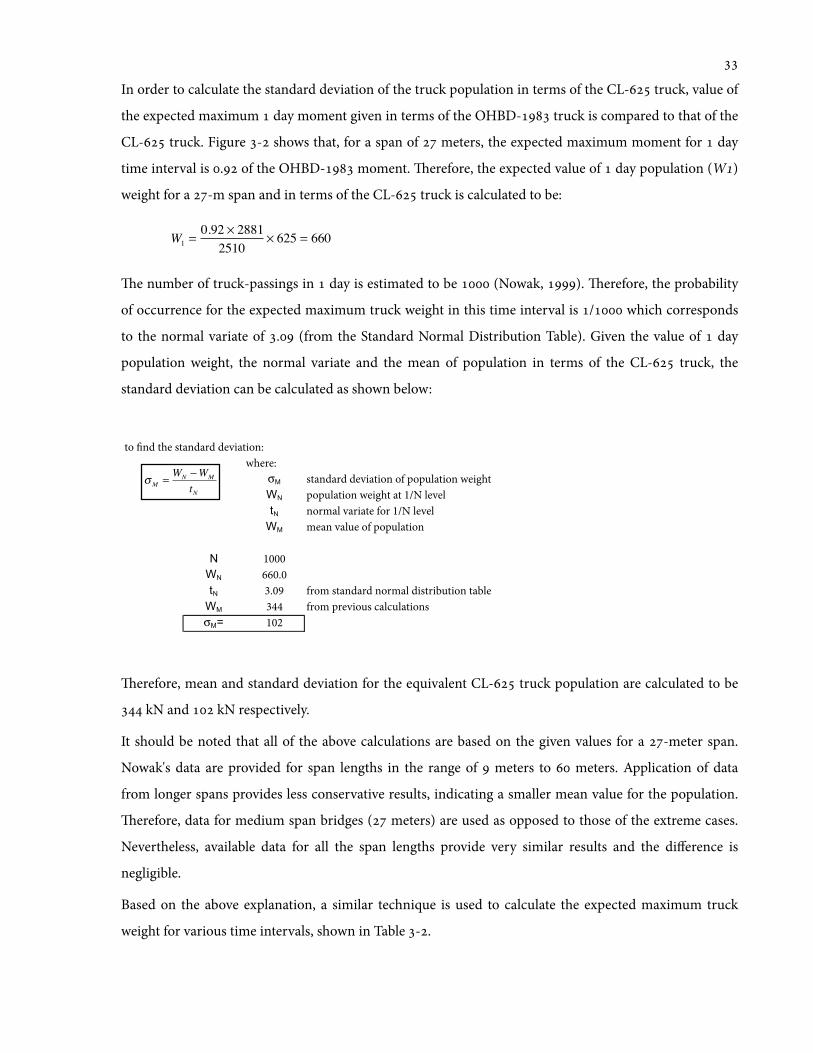
In order to calculate the standard deviation of the truck population in terms of the CL- truck, value of
the expected maximum day moment given in terms of the OHBD- truck is compared to that of the
CL- truck. Figure - shows that, for a span of meters, the expected maximum moment for day
time interval is . of the OHBD- moment. erefore, the expected value of day population (W)
weight for a -m span and in terms of the CL- truck is calculated to be:
W1 =0.92 × 28812510
× 625 = 660
e number of truck-passings in day is estimated to be (Nowak, ). erefore, the probability
of occurrence for the expected maximum truck weight in this time interval is / which corresponds
to the normal variate of . (from the Standard Normal Distribution Table). Given the value of day
population weight, the normal variate and the mean of population in terms of the CL- truck, the
standard deviation can be calculated as shown below:
erefore, mean and standard deviation for the equivalent CL- truck population are calculated to be
kN and kN respectively.
It should be noted that all of the above calculations are based on the given values for a -meter span.
Nowak's data are provided for span lengths in the range of meters to meters. Application of data
from longer spans provides less conservative results, indicating a smaller mean value for the population.
erefore, data for medium span bridges ( meters) are used as opposed to those of the extreme cases.
Nevertheless, available data for all the span lengths provide very similar results and the difference is
negligible.
Based on the above explanation, a similar technique is used to calculate the expected maximum truck
weight for various time intervals, shown in Table -.
to !nd the standard deviation:where:
!M standard deviation of population weightWN population weight at 1/N level tN normal variate for 1/N levelWM mean value of population
N 1000WN 660.0tN 3.09 from standard normal distribution tableWM 344 from previous calculations!M= 102
!M=W
N"W
M
tN
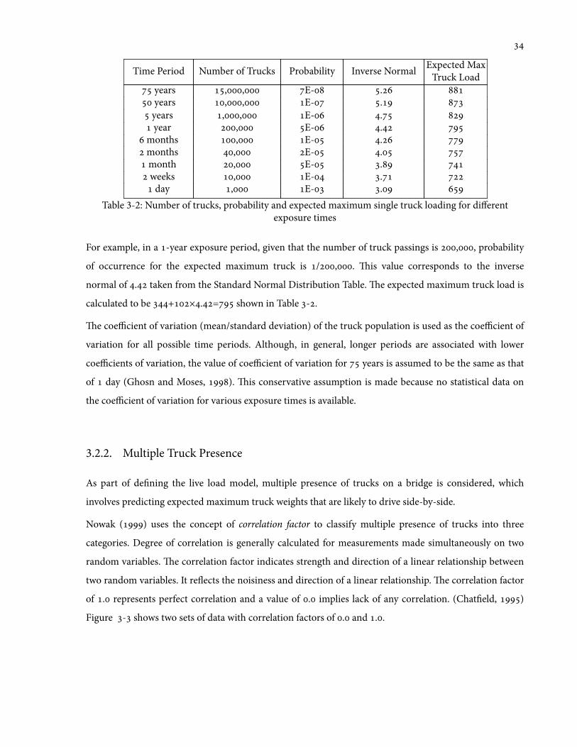
Time Period Number of Trucks Probability Inverse Normal Expected MaxTruck Load
years ,, E- . years ,, E- . years ,, E- . year , E- .
months , E- . months , E- . month , E- . weeks , E- .
day , E- . Table 3-2: Number of trucks, probability and expected maximum single truck loading for different
exposure times
For example, in a -year exposure period, given that the number of truck passings is ,, probability
of occurrence for the expected maximum truck is /,. is value corresponds to the inverse
normal of . taken from the Standard Normal Distribution Table. e expected maximum truck load is
calculated to be +×.= shown in Table -.
e coefficient of variation (mean/standard deviation) of the truck population is used as the coefficient of
variation for all possible time periods. Although, in general, longer periods are associated with lower
coefficients of variation, the value of coefficient of variation for years is assumed to be the same as that
of day (Ghosn and Moses, ). is conservative assumption is made because no statistical data on
the coefficient of variation for various exposure times is available.
3.2.2. Multiple Truck Presence
As part of de'ning the live load model, multiple presence of trucks on a bridge is considered, which
involves predicting expected maximum truck weights that are likely to drive side-by-side.
Nowak () uses the concept of correlation factor to classify multiple presence of trucks into three
categories. Degree of correlation is generally calculated for measurements made simultaneously on two
random variables. e correlation factor indicates strength and direction of a linear relationship between
two random variables. It re1ects the noisiness and direction of a linear relationship. e correlation factor
of . represents perfect correlation and a value of . implies lack of any correlation. (Chat'eld, )
Figure - shows two sets of data with correlation factors of . and ..
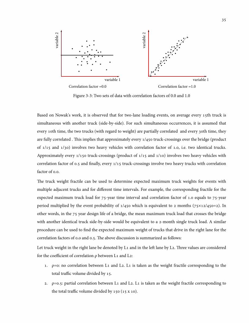
Figure 3-3: Two sets of data with correlation factors of 0.0 and 1.0
Based on Nowak's work, it is observed that for two-lane loading events, on average every th truck is
simultaneous with another truck (side-by-side). For such simultaneous occurrences, it is assumed that
every th time, the two trucks (with regard to weight) are partially correlated and every th time, they
are fully correlated . is implies that approximately every / truck-crossings over the bridge (product
of / and /) involves two heavy vehicles with correlation factor of ., i.e. two identical trucks.
Approximately every / truck-crossings (product of / and /) involves two heavy vehicles with
correlation factor of . and 'nally, every / truck-crossings involve two heavy trucks with correlation
factor of ..
e truck weight fractile can be used to determine expected maximum truck weights for events with
multiple adjacent trucks and for different time intervals. For example, the corresponding fractile for the
expected maximum truck load for -year time interval and correlation factor of . equals to -year
period multiplied by the event probability of / which is equivalent to months (×/=). In
other words, in the year design life of a bridge, the mean maximum truck load that crosses the bridge
with another identical truck side-by-side would be equivalent to a -month single truck load. A similar
procedure can be used to 'nd the expected maximum weight of trucks that drive in the right lane for the
correlation factors of .o and .. e above discussion is summarized as follows:
Let truck weight in the right lane be denoted by L and in the le lane by L. ree values are considered
for the coefficient of correlation ρ between L and L:
. ρ=: no correlation between L and L. L is taken as the weight fractile corresponding to the
total traffic volume divided by .
. ρ=.: partial correlation between L and L. L is taken as the weight fractile corresponding to
the total traffic volume divided by ( x ).
variable 1
varia
ble 2
varia
ble 2
variable 1Correlation factor =0.0 Correlation factor =1.0

. ρ=: full correlation between L and L. L is taken as the weight fractile corresponding to the
total traffic volume divided by ( x ).
e above assumptions are used to estimate truck weights in the right lane for the two-truck loading
events and various time intervals. In the case of full correlation, the two trucks are identical with the same
weight but for cases with correlation factors of . and ., truck weights in the le lane have yet to be
determined.
e available literature provides limited information on the expected traffic in the le lane. In addition,
load cases with correlation factors of . and . are generally ignored in current literature and two
identical side-by-side trucks are selected as the critical loading case. is is a conservative assumption
because probability of having two identical heavy trucks side-by-side is very slim and generally lighter
vehicles rather than heavy vehicles tend to pass in the fast lane. erefore, in order to arrive at a more
realistic traffic model, all three correlation factors are modeled in this study.
Based on simulations for -year truck loading performed by Nowak (), the average truck (kN)
and -day truck (kN) should be applied in the le lane for the correlation factors of . and .
respectively. Based on the de'nition of correlation factor on linear relationships between two random
variables, the ratio of the le lane truck weight to the right lane truck weight is assumed to be constant
(linear relation). Given this assumption and the -year truck loading values, the truck weight in the le
lane can be selected for other time intervals. In other words, possible two-truck loading events are
divided into three distinct groups, each modeled with a line passing through Nowak's -year loading
events as shown in Figure -. In this 'gure, the area on the le of the black line de'nes all the possible
loading events. It can be seen that instead of modeling possible loading cases by dividing the area equally
into three sections, a more conservative approach is taken and the two lines corresponding to correlation
factors of . and . are inclined towards a heavier “lighter truck.”
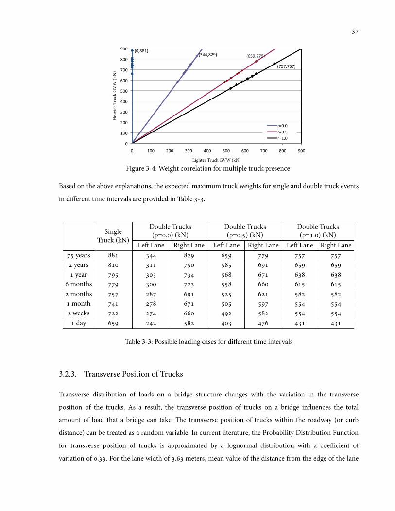
Figure 3-4: Weight correlation for multiple truck presence
Based on the above explanations, the expected maximum truck weights for single and double truck events
in different time intervals are provided in Table -.
SingleTruck (kN)
Double Trucks(ρ=.) (kN)
Double Trucks(ρ=.) (kN)
Double Trucks(ρ=.) (kN)
Le Lane Right Lane Le Lane Right Lane Le Lane Right Lane years years year
months months month weeks
day
Table 3-3: Possible loading cases for different time intervals
3.2.3. Transverse Position of Trucks
Transverse distribution of loads on a bridge structure changes with the variation in the transverse
position of the trucks. As a result, the transverse position of trucks on a bridge in1uences the total
amount of load that a bridge can take. e transverse position of trucks within the roadway (or curb
distance) can be treated as a random variable. In current literature, the Probability Distribution Function
for transverse position of trucks is approximated by a lognormal distribution with a coefficient of
variation of .. For the lane width of . meters, mean value of the distance from the edge of the lane
!"##$%&'() !*+'$,,'())
!,+,$,+,()
!-$%%.()
-)
.--)
&--)
"--)
#--)
+--)
*--)
,--)
%--)
'--)
-) .--) &--) "--) #--) +--) *--) ,--) %--) '--)
Hea
vier
Tru
ck G
VW (k
N()
Lighter Truck GVW (kN)
/0-1-)
/0-1+)
/0.1-)
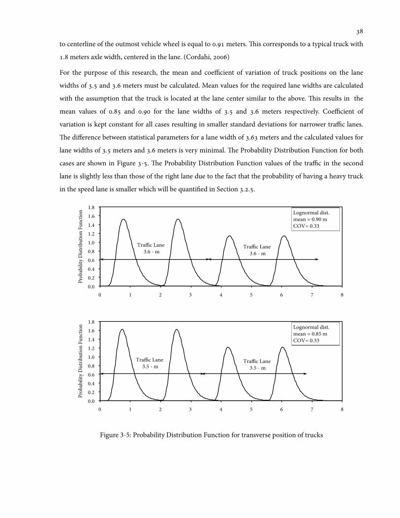
to centerline of the outmost vehicle wheel is equal to . meters. is corresponds to a typical truck with
. meters axle width, centered in the lane. (Cordahi, )
For the purpose of this research, the mean and coefficient of variation of truck positions on the lane
widths of . and . meters must be calculated. Mean values for the required lane widths are calculated
with the assumption that the truck is located at the lane center similar to the above. is results in the
mean values of . and . for the lane widths of . and . meters respectively. Coefficient of
variation is kept constant for all cases resulting in smaller standard deviations for narrower traffic lanes.
e difference between statistical parameters for a lane width of . meters and the calculated values for
lane widths of . meters and . meters is very minimal. e Probability Distribution Function for both
cases are shown in Figure -. e Probability Distribution Function values of the traffic in the second
lane is slightly less than those of the right lane due to the fact that the probability of having a heavy truck
in the speed lane is smaller which will be quanti'ed in Section ...
Figure 3-5: Probability Distribution Function for transverse position of trucks
0.0 0.2 0.4 0.6 0.8 1.0 1.2 1.4 1.6 1.8
0 1 2 3 4 5 6 7 8
Prob
abili
ty D
istrib
utio
n Fu
nctio
n
Tra!c Lane 3.6 - m
Lognormal dist. mean = 0.85 m COV= 0.29
Lognormal dist. mean = 0.85 m COV= 0.29
Lognormal dist. mean = 0.85 m COV= 0.29
Lognormal dist. mean = 0.85 m COV= 0.29
Lognormal dist. mean = 0.85 m COV= 0.29
Lognormal dist. mean = 0.90 m COV= 0.33
Tra!c Lane 3.6 - m
0.0 0.2 0.4 0.6 0.8 1.0 1.2 1.4 1.6 1.8
0 1 2 3 4 5 6 7 8
Prob
abili
ty D
istrib
utio
n Fu
nctio
n
Tra!c Lane 3.5 - m
Lognormal dist. mean = 0.85 m COV= 0.29
Lognormal dist. mean = 0.85 m COV= 0.29
Lognormal dist. mean = 0.85 m COV= 0.29
Lognormal dist. mean = 0.85 m COV= 0.29
Lognormal dist. mean = 0.85 m COV= 0.29
Lognormal dist. mean = 0.85 m COV= 0.33
Tra!c Lane 3.5 - m
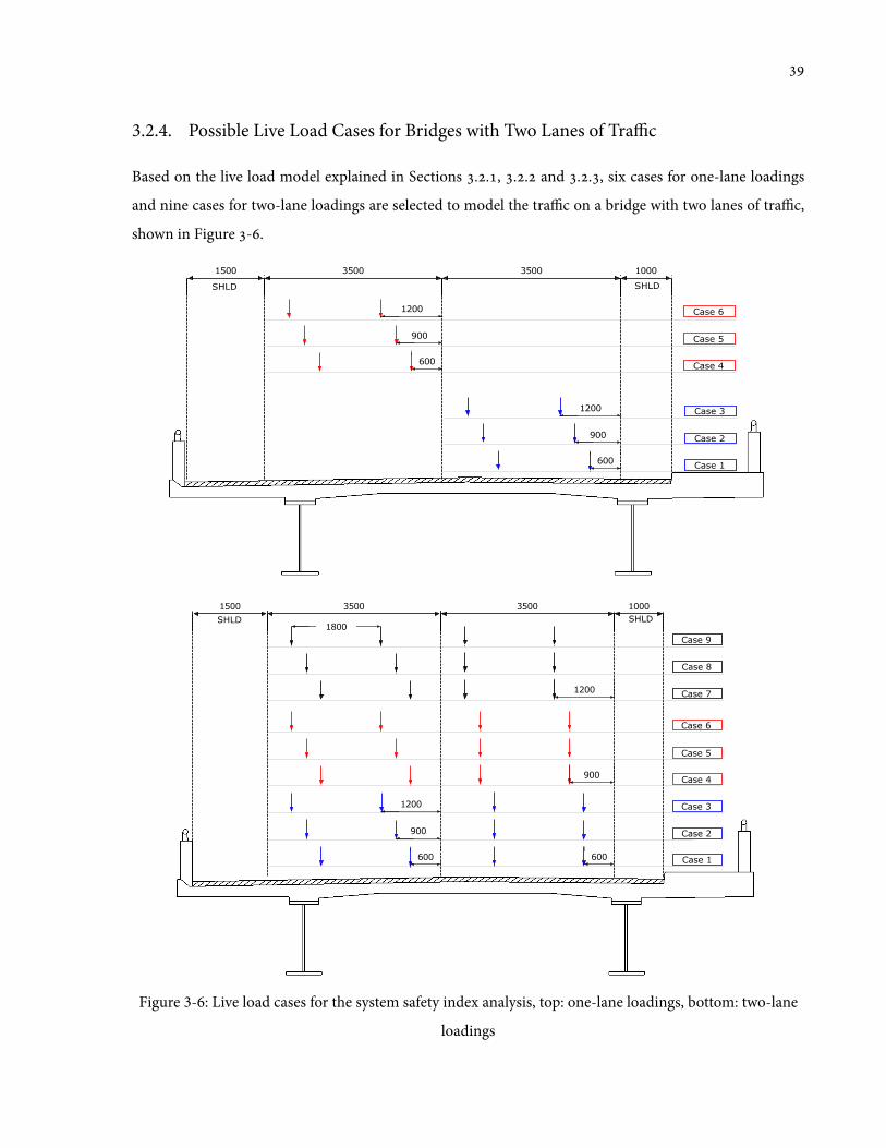
3.2.4. Possible Live Load Cases for Bridges with Two Lanes of Traffic
Based on the live load model explained in Sections .., .. and .., six cases for one-lane loadings
and nine cases for two-lane loadings are selected to model the traffic on a bridge with two lanes of traffic,
shown in Figure -.
Figure 3-6: Live load cases for the system safety index analysis, top: one-lane loadings, bottom: two-lane
loadings
1500 3500 3500 1000
SHLD SHLD
Case 1
Case 2
Case 3
Case 4
Case 5
Case 6
900
1200
600
900
1200
600
1500 3500 3500 1000
900
600
1200
900
1200
600
SHLD SHLD1800
Case 1
Case 2
Case 3
Case 4
Case 5
Case 6
Case 7
Case 8
Case 9
ree different positions are selected to model transverse location of a truck in a traffic lane: ., . and
. meters from the edge of the traffic lane. In one-lane loadings, the truck is located either in the right
lane or the le lane. e truck weight is obtained based on the assumed time interval summarized in
Table - on page . In two-lane loading cases, the trucks in a traffic lane may take any of the assumed
three positions shown in Figure -. erefore, a total of nine loading events cover all the possible cases.
Truck weight in the right traffic lane can be obtained based on the assumed time intervals given in
Section .. and truck weight in the le traffic lane depends on the correlation factor between the two
trucks. ree possible correlation factors are incorporated in the model for every two-lane loading event,
resulting in a total of two side-by-side truck events on the bridge. In summary, a total of live load
cases will be considered to model loads on a bridge with two lanes of traffic.
3.2.5. Probability of Occurrence for Live Load Events
In the calculation of the system safety index at the ultimate state, the NCHRP Report No. guidelines
de'ne the maximum expected load for both intact and damaged bridges in terms of a multiple of two
standard side-by-side trucks. e reason behind selection of two identical side-by-side trucks as the
reference load con'guration is due to the fact that this loading event is found to be the critical loading
case for many two-lane bridges and creates the maximum effect at a critical location. (Ghosn and Moses,
)
Studies of heavy traffic patterns on bridges show that the probability of having two completely correlated
side-by-side trucks is considerably lower than the probability of single truck events or side-by-side trucks
with partial correlations. Given the above, in this thesis, system safety index for both intact and damaged
conditions is calculated for all possible loading events (single and multiple trucks). In addition,
probability of occurrence for every possible loading event is determined. is way, a weighted average
system safety index can be calculated which provides a more realistic estimate for the system safety index.
For two-lane bridges, a total of 've loading events, described in Section .., are considered. For single
truck loading events, of trucks are assumed to drive in the right lane and move in the le lane
(Ressler, ). Probability values for the multiple truck loading events are based on the work of Nowak
() and the assumptions described in Section .. which are summarized below:
. Lane position histogram for single truck events:
. Right Lane: .;
. Le Lane: ..
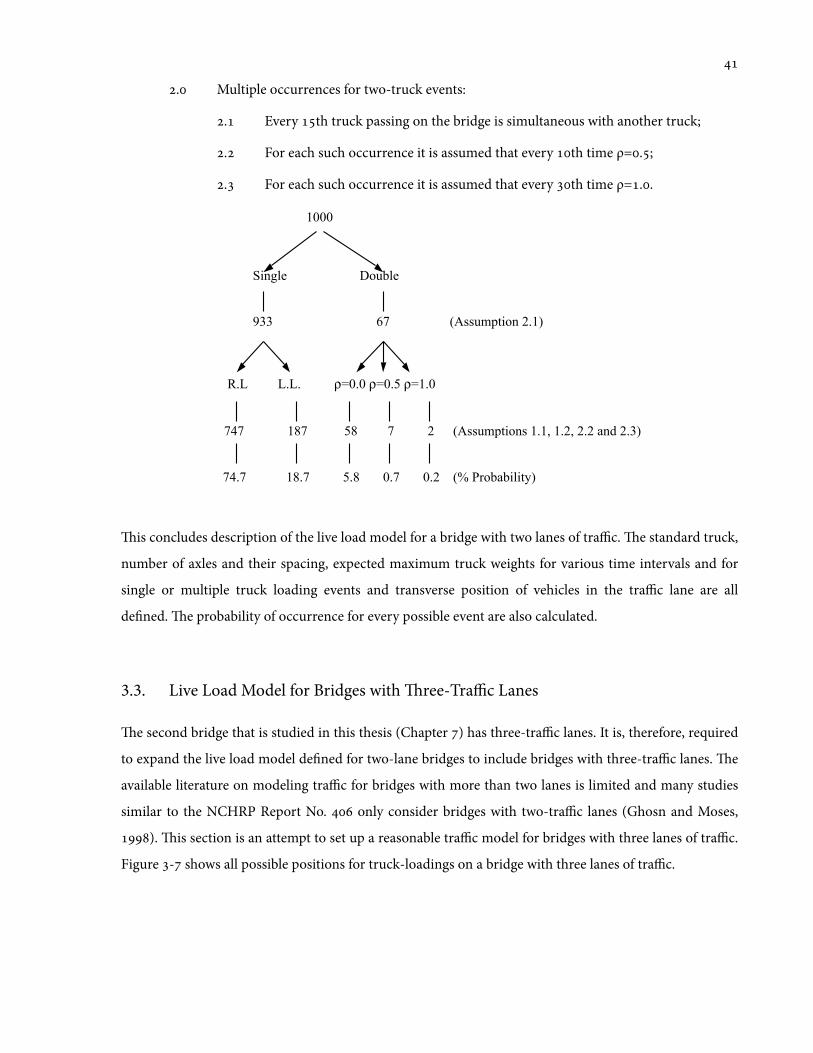
. Multiple occurrences for two-truck events:
. Every th truck passing on the bridge is simultaneous with another truck;
. For each such occurrence it is assumed that every th time ρ=.;
. For each such occurrence it is assumed that every th time ρ=..
is concludes description of the live load model for a bridge with two lanes of traffic. e standard truck,
number of axles and their spacing, expected maximum truck weights for various time intervals and for
single or multiple truck loading events and transverse position of vehicles in the traffic lane are all
de'ned. e probability of occurrence for every possible event are also calculated.
3.3. Live Load Model for Bridges with ree-Traffic Lanes
e second bridge that is studied in this thesis (Chapter ) has three-traffic lanes. It is, therefore, required
to expand the live load model de'ned for two-lane bridges to include bridges with three-traffic lanes. e
available literature on modeling traffic for bridges with more than two lanes is limited and many studies
similar to the NCHRP Report No. only consider bridges with two-traffic lanes (Ghosn and Moses,
). is section is an attempt to set up a reasonable traffic model for bridges with three lanes of traffic.
Figure - shows all possible positions for truck-loadings on a bridge with three lanes of traffic.
1000
Single Double
933 67 (Assumption 2.1)
R.L L.L. !=0.0 !=0.5 !=1.0
747 187 58 7 2 (Assumptions 1.1, 1.2, 2.2 and 2.3)
74.7 18.7 5.8 0.7 0.2 (% Probability)

Figure 3-7: Possible truck positions on a bridge with three lanes of traffic
In this 'gure, there are four more possible loading events than those considered for a two-lane bridge:
Case : One truck in lane
Case : Two side-by-side trucks in lanes and
Case : Two trucks in lanes and
Case : ree side-by side trucks
It is assumed that Cases “,” “” and “” would rarely happen (due to traffic regulations) and as a result
can be excluded from the model. In design of bridges, three identical side-by-side truck loadings are
considered to be one possible loading case; therefore, to be consistent with design standards, Case is
included in the live load model.
Given the above discussion on possible loading cases, the following questions have to be answered in
order to de'ne the live load model for bridges with three lanes of traffic:
. Are the truck weights and the assumed statistics de'ned for the load cases of two-lane
bridges applicable to bridges with three lanes of traffic?
. What are the truck weight values for three side-by-side trucks?
. What is the probability of occurrence for single, double or triple truck events?
ese questions are brie1y answered below:
In a recent study in the United States, attempts have been made to verify the current AASHTO LRFD
design code speci'cations for the maximum live load on highway bridges. In this study visual data
collected from traffic cameras are coupled with the structural strain response of a steel girder bridge
located on I- in Delaware (Guzda et al., ). e bridge is located in an area with high average daily
truck traffic and has four traffic lanes. Frequency of multiple presence of truck traffics in adjacent lanes
was recorded. e study shows that approximately . of traffic-passings involved two trucks within
adjacent lanes while separated by a distance of less than two truck lengths, and . of trucks traveled
side-by-side with headway distance of one truck length.
Lane 1
Lane 2
Lane 3
Case 1 Case 2 Case 3 Case 4 Case 5 Case 6 Case 7
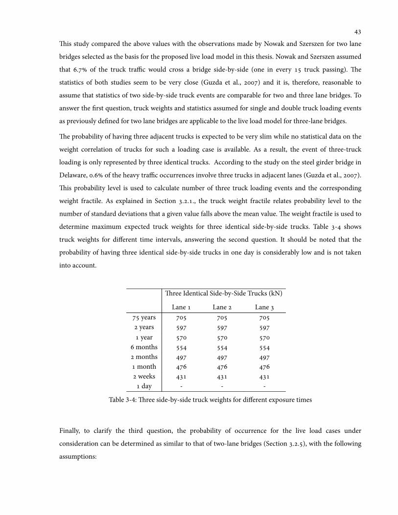
is study compared the above values with the observations made by Nowak and Szerszen for two lane
bridges selected as the basis for the proposed live load model in this thesis. Nowak and Szerszen assumed
that . of the truck traffic would cross a bridge side-by-side (one in every truck passing). e
statistics of both studies seem to be very close (Guzda et al., ) and it is, therefore, reasonable to
assume that statistics of two side-by-side truck events are comparable for two and three lane bridges. To
answer the 'rst question, truck weights and statistics assumed for single and double truck loading events
as previously de'ned for two lane bridges are applicable to the live load model for three-lane bridges.
e probability of having three adjacent trucks is expected to be very slim while no statistical data on the
weight correlation of trucks for such a loading case is available. As a result, the event of three-truck
loading is only represented by three identical trucks. According to the study on the steel girder bridge in
Delaware, . of the heavy traffic occurrences involve three trucks in adjacent lanes (Guzda et al., ).
is probability level is used to calculate number of three truck loading events and the corresponding
weight fractile. As explained in Section ..., the truck weight fractile relates probability level to the
number of standard deviations that a given value falls above the mean value. e weight fractile is used to
determine maximum expected truck weights for three identical side-by-side trucks. Table - shows
truck weights for different time intervals, answering the second question. It should be noted that the
probability of having three identical side-by-side trucks in one day is considerably low and is not taken
into account.
ree Identical Side-by-Side Trucks (kN)
Lane Lane Lane years years year
months months month weeks
day - - -
Table 3-4: ree side-by-side truck weights for different exposure times
Finally, to clarify the third question, the probability of occurrence for the live load cases under
consideration can be determined as similar to that of two-lane bridges (Section ..), with the following
assumptions:
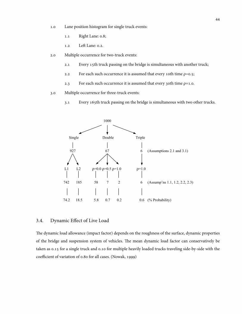
. Lane position histogram for single truck events:
. Right Lane: .;
. Le Lane: ..
. Multiple occurrence for two-truck events:
. Every th truck passing on the bridge is simultaneous with another truck;
. For each such occurrence it is assumed that every th time ρ=.;
. For each such occurrence it is assumed that every th time ρ=..
. Multiple occurrence for three-truck events:
. Every th truck passing on the bridge is simultaneous with two other trucks.
3.4. Dynamic Effect of Live Load
e dynamic load allowance (impact factor) depends on the roughness of the surface, dynamic properties
of the bridge and suspension system of vehicles. e mean dynamic load factor can conservatively be
taken as . for a single truck and . for multiple heavily loaded trucks traveling side-by-side with the
coefficient of variation of . for all cases. (Nowak, )
1000
Single Double Triple
927 67 6 (Assumptions 2.1 and 3.1)
L1 L2 !=0.0 !=0.5 !=1.0 !=1.0
742 185 58 7 2 6 (Assump’ns 1.1, 1.2, 2.2, 2.3)
74.2 18.5 5.8 0.7 0.2 0.6 (% Probability)

3.5. Expected Live Loads in the Safety Index Formula
Design life of a bridge is generally assumed to be years. erefore, in case of intact bridges, system-
level safety index at the ultimate is calculated based on -year loading events.
A bridge in damaged condition should withstand regular traffic until closure time. In current literature
and the NCHRP Report No. , the expected load for damaged condition is determined based on the -
year time interval (Ghosn and Moses, ). e reason behind this selection is based on the biennial
mandatory bridge inspection interval. It is believed that even if the damage goes unnoticed for a short
time, it is bound to be noticed during the mandatory inspection and a proper action will be taken.
(Ghosn and Moses, )
e objective of this study is that in the case of a sudden brittle failure of a load-carrying component, the
bridge should withstand progressive failure or collapse until closure to traffic. In such cases, damage
should be noticed sooner than years as behavior of the bridge will possibly change and de1ections
become noticeable. erefore, it is suggested that the safety index of damaged bridges be calculated for
different possible exposure times and estimate probability of detecting damage for such time intervals.
is leads to the calculation of a weighted average safety index that re1ects reliability of the damaged
system more realistically.
In order to calculate probability of detecting damage for a given exposure time, the number of load
applications between failure of a bridge component (e.g. a girder) and the damage detection is
represented by a random variable NG-D. Probability of damage detection increases with time as more
vehicles cross the bridge.
e cumulative distribution function FNG−D(n) can be modeled for the variable NG-D using geometric
distribution. e geometric distribution in the probability theory is de'ned as the number of trials (i.e.
truck passings) needed to get one success (i.e. damage detection). In this study, the number of truck-
passings required to detect damage is related to the probability of damage detection for a single load
application. e cumulative distribution of such function can be formulated as given in Equation -,
where "n" is the number of load applications at the time of interest, Pd is the probability of damage
detection for a single load application and nd is the prescribed interval that the damage is bound to be
detected which is stated in terms of load application. (Ressler, )

FNG−D(n) =
1
1−(1−Pd )n
forn≥nd
for0≤n≤nd⎧⎨⎪
⎩⎪
⎫⎬⎪
⎭⎪Equation -
As previously discussed, available literature requires a bridge under damaged condition to be analyzed for
the expected -year traffic load. It seems that current procedures for system reliability analysis of bridges
tend to conservatively generalize the estimation of safety index for damaged bridges (Ghosn and Moses,
) and (Ressler, ). Damage in a component of the bridge can be detected by official inspections or
by change in the behavior of the bridge, namely de1ections noticeable to the public. In the above
distribution function, nd (the interval during which damaged component is bound to be discovered) can
be estimated based on bridge de1ections aer a component fails. Knowing the level of de1ections that are
noticeable and the load-de1ection response of a bridge, the corresponding load and consequently number
of load applications n that ensures damage detection can be estimated. FNG-D in Equation - is equal to
. for such estimated value of n. One possible solution for Equation - is now found and value of Pd
can be calculated. Once the value of Pd is obtained, FNG-D can be determined for every other given value of
n.
As an example, Table - shows probability of damage detection for various time intervals when
damage detection time is years (nd= years). Also, Figure - compares probability of damage detection
for various exposure times when nd equals: years, year, months or months.
Table 3-5: Probability of damage detection for various exposure times when nd=2 years
Pd Exposure Time No. of Truck Passings
Prob. of Damage Detection
1.876E-05 75 years 15,000,000 1.0050 years 10,000,000 1.005 years 1,000,000 1.002 years 400,000 1.001 year 200,000 0.98
6 months 100,000 0.852 months 40,000 0.531 month 20,000 0.312 weeks 10,000 0.17
1 day 1,000 0.02
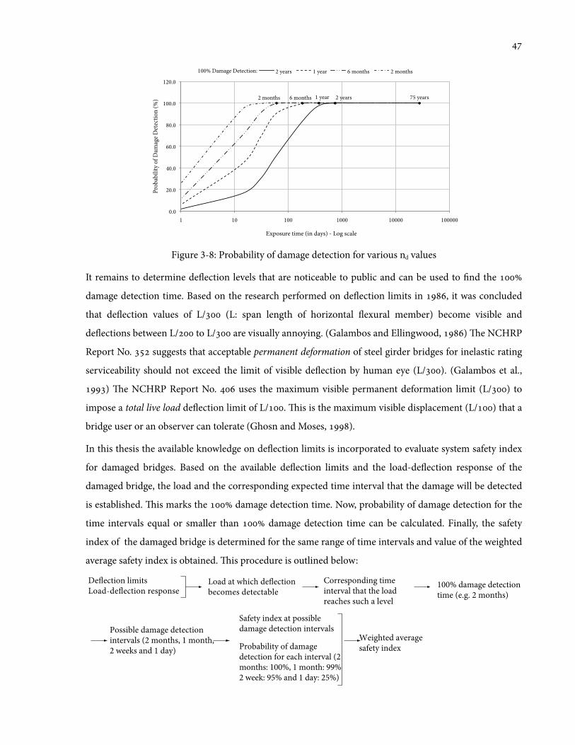
Figure 3-8: Probability of damage detection for various nd values
It remains to determine de1ection levels that are noticeable to public and can be used to 'nd the
damage detection time. Based on the research performed on de1ection limits in , it was concluded
that de1ection values of L/ (L: span length of horizontal 1exural member) become visible and
de1ections between L/ to L/ are visually annoying. (Galambos and Ellingwood, ) e NCHRP
Report No. suggests that acceptable permanent deformation of steel girder bridges for inelastic rating
serviceability should not exceed the limit of visible de1ection by human eye (L/). (Galambos et al.,
) e NCHRP Report No. uses the maximum visible permanent deformation limit (L/) to
impose a total live load de1ection limit of L/. is is the maximum visible displacement (L/) that a
bridge user or an observer can tolerate (Ghosn and Moses, ).
In this thesis the available knowledge on de1ection limits is incorporated to evaluate system safety index
for damaged bridges. Based on the available de1ection limits and the load-de1ection response of the
damaged bridge, the load and the corresponding expected time interval that the damage will be detected
is established. is marks the damage detection time. Now, probability of damage detection for the
time intervals equal or smaller than damage detection time can be calculated. Finally, the safety
index of the damaged bridge is determined for the same range of time intervals and value of the weighted
average safety index is obtained. is procedure is outlined below:
75 years 2 years 1 year 6 months 2 months
100% Damage Detection:
0.0
20.0
40.0
60.0
80.0
100.0
120.0
1 10 100 1000 10000 100000
Prob
abili
ty o
f Dam
age D
etec
tion
(%)
Exposure time (in days) - Log scale
2 years 1 year 6 months 2 months
De!ection limitsLoad-de!ection response
Load at which de!ection becomes detectable
Corresponding time interval that the load reaches such a level
100% damage detection time (e.g. 2 months)
Possible damage detection intervals (2 months, 1 month, 2 weeks and 1 day)
Safety index at possible damage detection intervals
Probability of damage detection for each interval (2 months: 100%, 1 month: 99% 2 week: 95% and 1 day: 25%)
Weighted average safety index
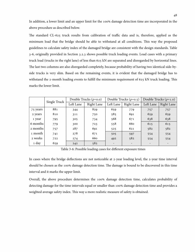
In addition, a lower limit and an upper limit for the damage detection time are incorporated in the
above procedure as described below.
e standard CL- truck results from calibration of traffic data and is, therefore, applied as the
minimum load that the bridge should be able to withstand at all conditions. is way the proposed
guidelines to calculate safety index of the damaged bridge are consistent with the design standards. Table
-, originally provided in Section .. shows possible truck loading events. Load cases with a primary
truck load (trucks in the right lane) of less than kN are separated and disregarded by horizontal lines.
e last two columns are also disregarded completely, because probability of having two identical side-by-
side trucks is very slim. Based on the remaining events, it is evident that the damaged bridge has to
withstand the -month loading events to ful'll the minimum requirement of kN truck loading. is
marks the lower limit.
Single TruckDouble Trucks (ρ=.) Double Trucks (ρ=.) Double Trucks (ρ=.)
Le Lane Right Lane Le Lane Right Lane Le Lane Right Lane years years year
months months month weeks
day - - - -
Table 3-6: Possible loading cases for different exposure times
In cases where the bridge de1ections are not noticeable at -year loading level, the -year time interval
should be chosen as the damage detection time. e damage is bound to be discovered in this time
interval and it marks the upper limit.
Overall, the above procedure determines the damage detection time, calculates probability of
detecting damage for the time intervals equal or smaller than damage detection time and provides a
weighted average safety index. is way a more realistic measure of safety is obtained.

Chapter 4
e Acceptable Probability of Failure
In this chapter, an acceptable range for probability of failure of bridges at the system level is determined.
e following topics will be addressed in this chapter:
() A brief overview of current available guidelines, from various organizations and sources, on
the adequate level of failure probability for a structural system;
() An appropriate probability of failure and level of redundancy applicable to bridge structural
systems for the purpose of this thesis.
One of the challenges in the reliability analysis of structures is to decide on an optimum probability of
failure. On the one hand, there is a trade off between cost and safety, where higher safety implies an
increase in cost. On the other hand, risk of failure should be de'ned for the bene't of public and the
decision on the minimum level of safety should be acceptable to the society. In general, when there is an
accident or a bridge fails society tends to react furiously and concerns arise over the safety of structures.
ere is always a tendency to overreact and accept higher costs to obtain increased safety; but as time
passes, optimum economical solutions become priority again. It is important to avoid inconsistencies in
the application of safety measures and agree upon an acceptable level of safety.

It seems that the easiest way for society and specialists to communicate about safety is the Probability of
Failure rather than the Safety Index.
e outcome of the procedure to calculate redundancy of a bridge at the system level described in
Chapters and , is two safety index values. By de'nition, safety index can be easily related to the
probability of failure:
β = Φ−1(1− Pf ) Equation -
e standard normal distribution table can be used to 'nd failure probability values of the calculated
safety indices from reliability analysis.
4.1. Joint Committee of Structural Safety (JCSS) Provisions
According to the document “Risk Acceptance Criteria,” published by the Joint Committee of Structural
Safety (JCSS) (Diamantidis, ), certain criteria such as the individual risk, societal risk and cost-
bene't analysis can be used to quantify or provide a comparison tool for safety assessment of structural
systems. e JCSS report classi'es these criteria into two categories:
. Human Safety approach:
a) Individual risk criteria:
“No individual (or group of individuals) involved in a particular activity can be exposed to an
unacceptable risk. If an individual (or group of individuals) is found to be exposed to excessive
risk, safety measures are adopted regardless of the cost-bene't effectiveness.” (Diamantidis,
)
b) Societal risk criteria:
“A certain activity must not produce high frequency occurrences of large-scale accidents (i.e.
with particularly severe consequences). In other words, the unacceptable level of risk varies for
different accident sizes. is principle tries to capture a supposed socio-political aversion to
large accidents and provides a regulatory basis (i.e. enforced investments in safety) in situations
where the two other criteria do not call for intervention.” (Diamantidis, )
. Safety Cost-Bene"t approach:
“e possible investments in safety measures are analyzed in terms of the expected bene'ts
(typically the prevention of a statistical fatality or serviceability failure). Only solutions with
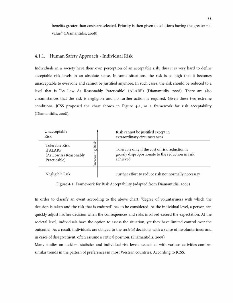
bene'ts greater than costs are selected. Priority is then given to solutions having the greater net
value.” (Diamantidis, )
4.1.1. Human Safety Approach - Individual Risk
Individuals in a society have their own perception of an acceptable risk; thus it is very hard to de'ne
acceptable risk levels in an absolute sense. In some situations, the risk is so high that it becomes
unacceptable to everyone and cannot be justi'ed anymore. In such cases, the risk should be reduced to a
level that is “As Low As Reasonably Practicable” (ALARP) (Diamantidis, ). ere are also
circumstances that the risk is negligible and no further action is required. Given these two extreme
conditions, JCSS proposed the chart shown in Figure -, as a framework for risk acceptability
(Diamantidis, ).
Figure 4-1: Framework for Risk Acceptability (adapted from Diamantidis, )
In order to classify an event according to the above chart, “degree of voluntariness with which the
decision is taken and the risk that is endured” has to be considered. At the individual level, a person can
quickly adjust his/her decision when the consequences and risks involved exceed the expectation. At the
societal level, individuals have the option to assess the situation, yet they have limited control over the
outcome. As a result, individuals are obliged to the societal decisions with a sense of involuntariness and
in cases of disagreement, oen assume a critical position. (Diamantidis, )
Many studies on accident statistics and individual risk levels associated with various activities con'rm
similar trends in the pattern of preferences in most Western countries. According to JCSS:
Unacceptable Risk
Tolerable Risk if ALARP (As Low As Reasonably Practicable)
Negligible Risk
Incr
easin
g Risk
Risk cannot be justi!ed except inextraordinary circumstances
Tolerable only if the cost of risk reduction isgrossly disproportionate to the reduction in riskachieved
Further e"ort to reduce risk not normally necessary

“ e probability of losing one’s life in normal daily activities such as driving a car or working in a
factory appears to be one or two orders of magnitude lower than the overall probability of dying.
Only a purely voluntary activity such as mountaineering entails a higher risk.”
Based on the results of such studies on public tolerance and voluntary and involuntary activities, an
acceptable probability of failure is proposed:
Pfi =βi .10
−4
Pd fi
Equation -
where Pd⎮" denotes the probability of being killed in the event of an accident. In this expression the policy
factor βi varies with the degree of voluntariness with which an activity i is undertaken and with the
bene't perceived. It ranges from , in the case of complete freedom of choice like mountaineering, to
. in the case of an imposed risk without any perceived direct bene't. A proposal for selection of the
value of the policy factor βi as a function of voluntariness and bene't is given in Table -. (Diamantidis,
)
βi Voluntariness Direct bene't Example
Completely voluntary Direct bene't Mountaineering Voluntary Direct bene't Motorbike riding. Neutral Direct bene't Car driving. Involuntary Some bene't Working in a factory. Involuntary No bene't Working in an LNG-plant
Table 4-1: Policy factor as a function of voluntariness and bene't (adapted from Diamantidis, 2008)
4.1.2. Human Safety Approach - Societal Risk
In this approach, the total damage due to an accident or a failure is quanti'ed as a collective risk for the
society as a whole. e collective risk considers all the individual risks involved in a given system
(Diamantidis, ). In the mathematical formulation, the consequences of a hazard is expressed as
fatalities per year and the hazard itself is classi'ed based on the frequency of occurrence. Generally, an F-
N curve (N represents number of fatalities and F frequency of accidents with more than N fatalities) is
generated in which an upper bound is selected for risks that can be tolerated while a lower bound shows
risks that are too low to be considered, shown in Figure - (Diamantidis, ). Such acceptability
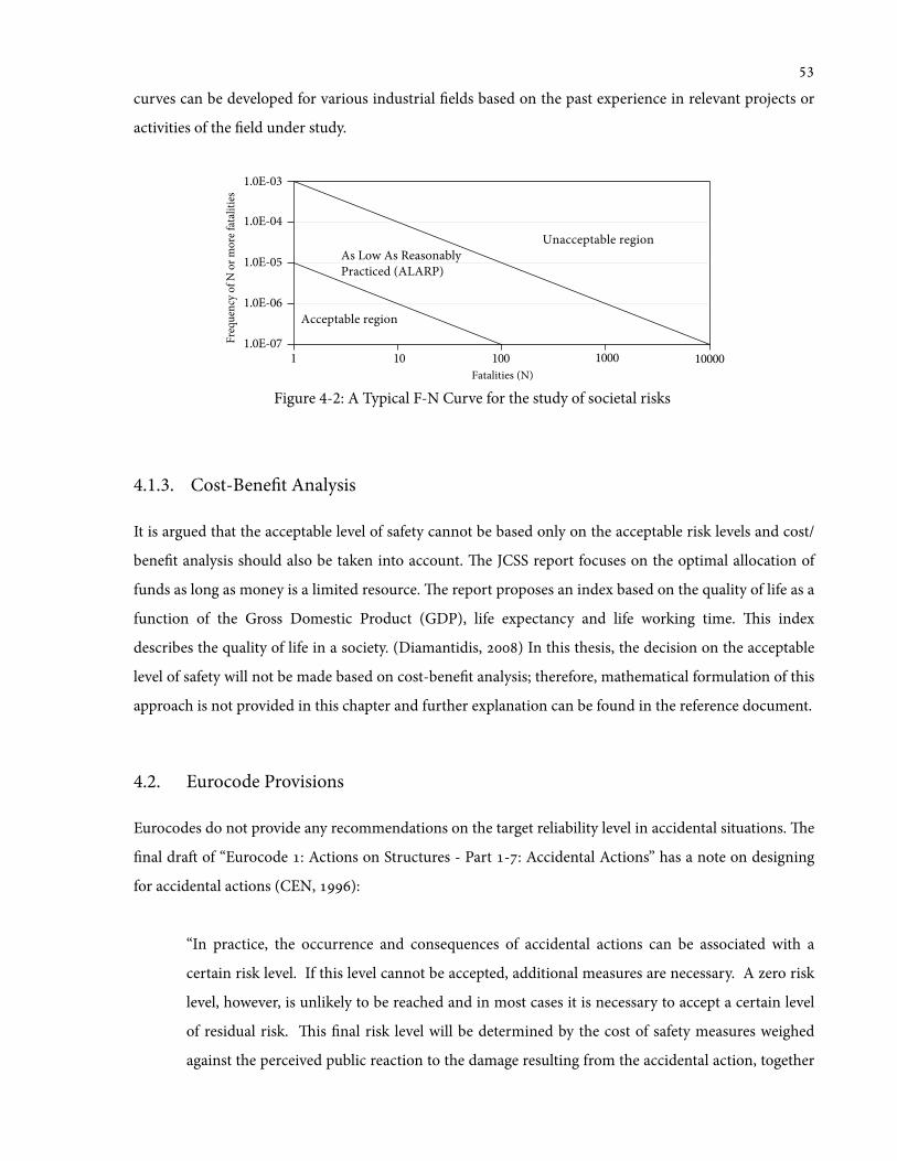
curves can be developed for various industrial 'elds based on the past experience in relevant projects or
activities of the 'eld under study.
Figure 4-2: A Typical F-N Curve for the study of societal risks
4.1.3. Cost-Bene't Analysis
It is argued that the acceptable level of safety cannot be based only on the acceptable risk levels and cost/
bene't analysis should also be taken into account. e JCSS report focuses on the optimal allocation of
funds as long as money is a limited resource. e report proposes an index based on the quality of life as a
function of the Gross Domestic Product (GDP), life expectancy and life working time. is index
describes the quality of life in a society. (Diamantidis, ) In this thesis, the decision on the acceptable
level of safety will not be made based on cost-bene't analysis; therefore, mathematical formulation of this
approach is not provided in this chapter and further explanation can be found in the reference document.
4.2. Eurocode Provisions
Eurocodes do not provide any recommendations on the target reliability level in accidental situations. e
'nal dra of “Eurocode : Actions on Structures - Part -: Accidental Actions” has a note on designing
for accidental actions (CEN, ):
“In practice, the occurrence and consequences of accidental actions can be associated with a
certain risk level. If this level cannot be accepted, additional measures are necessary. A zero risk
level, however, is unlikely to be reached and in most cases it is necessary to accept a certain level
of residual risk. is 'nal risk level will be determined by the cost of safety measures weighed
against the perceived public reaction to the damage resulting from the accidental action, together
1 10 100 1000 100001.0E-07
1.0E-06
1.0E-05
1.0E-04
1.0E-03
Unacceptable region
Acceptable region
As Low As Reasonably Practiced (ALARP)
Fatalities (N)
Freq
uenc
y of N
or m
ore f
atali
ties
with consideration of the economic consequences and the potential number of casualties
involved. e risk should also be based on a comparison with risks generally accepted by society
in comparable situations.”
According to Eurocode : Part -, the structures are classi'ed into three classes considering the possible
consequences of failure (CEN, ):
Class CC (low consequences): no special requirements are needed with respect to accidental actions
except to ensure that the basic rules for robustness and stability are met.
Class CC (medium consequences): a simpli'ed analysis by static equivalent action models may be
adopted or prescriptive design/detailing rules applied.
Class CC (high consequences): examination of the speci'c case should be carried out to determine the
level of reliability and the depth of structural analysis (risk assessment, non-linear or dynamic analysis).
e decision on the appropriate method of analysis or measures that should be taken depends on which
one of the above classes best suits the situation. e decision on selection of the relevant class for a
structure is le to the European member states (CEN, ).
4.3. International Organization for Standardization
According to Vrouwenvelder (), the International Organization for Standardization (ISO) prepared a
document in titled “DIS : General principles on reliability for structures.” Vrouwenvelder
() studied modeling of extreme actions in structural engineering in a paper. He states that
economical optimizations are not always the answer to the problem of human safety and refers to ISO's
formulation for acceptable levels of failure probability. According to ISO-DIS , the annual maximum
accepted probability of structural failure based on limiting individual risk may be expressed as
(Vrouwenvelder, ):
Pf <10−6
P(d f )Equation -
where P(d⎮f) is the probability of casualties in a given structural failure which depends on the time a
person spends in or around a certain structure.
Also, when the societal risk is considered, the annual maximal probability of structural failure may be
expressed as:(Vrouwenvelder, )
Pf < AN−k Equation -

Where N is the expected number of fatalities per year. A and k are constant values with A in the range of
./year to ./year and k in the range of to . Higher values of k indicates the social aversion to large
disasters. In cases when the number of fatalities N in an event of failure is highly uncertain, the failure
probability can be expressed as:
P(N > n) < An−k Equation -
is relation should hold for all values of n.
4.4. e NCHRP Report No. 406 Guidelines
e NCHRP Report No. provides minimum target reliability indices that are based on the
performance of existing redundant bridges (Ghosn and Moses, ). e study includes multi-girder
steel bridges, prestressed concrete I-beam bridges, prestressed concrete multibox beam bridges and
prestressed concrete spread box-girder bridges. In the NCHRP Report No. , two and three-girder
bridges are considered to be non-redundant and target reliability indices are determined based on the
behavior of four-girder bridges.
e database used in this study shows that two-lane bridges designed according to the AASHTO
LFD criteria with the HS- loading are adequately redundant when their ultimate system safety index
exceeds .. is is based on the assumption that components of such systems have safety index of .. It
also concludes that the damaged system safety index of . satis'es requirements of a redundant bridge
structure. (Ghosn and Moses, )
4.5. Acceptable Level of Redundancy
e decision on the acceptable level of redundancy for bridges requires comprehensive study of different
factors. Considering consequences of a bridge failure, society in general and policy makers in particular
are also involved in deciding on an acceptable probability of failure; therefore, this is not entirely an
engineering matter. In this section, a brief discussion is provided to evaluate a range of acceptable
reliability levels for the purpose of this thesis.
Sections . to . are the most commonly quoted guidelines in the current literature and they all provide
a similar value of ⁶ as an acceptable level of annual probability of failure for important bridge
structures (Duckett, ). Based on the cost-bene't analysis and the study of existing structures, it is
recommended to reduce the above value to ⁴ (Duckett, ). Given these values are provided on
annual basis, it is reasonable to assume that the acceptable probability of failure for the design life of a

bridge ( years) should be larger. is is due to the fact that as the time interval increases, the chances
that the bridge fails are larger. In addition, the NCHRP Report No. speci'es the minimum acceptable
ultimate and damage system safety indices of . and . corresponding to the failure probability values
of .x⁶ and .x1 respectively. is implies that a conservative approach is adapted by the NCHRP
by selecting the -year failure probability of a bridge in the order of ⁶ while other available guidelines
choose the same range of acceptable failure probability for annual basis.
It should be noted that the design load and resistance factors provided in the Canadian Highway Bridge
Design Code (CHBDC) or the AASHTO LRFD Bridge Design speci'cations guarantee a value of . for
β at the component level. is implies that components of a structural system will have a failure
probability of .x⁴. It should be noted that the probability of failure of a redundant system is smaller
than the probability of failure of its members.
It seems that at present, no universally accepted values or a rational method to decide on the failure
probability of structural systems and bridges in particular have been agreed on. Given the limitations of
the available guidelines and taking a conservative approach for the purpose of this thesis, the probability
of failure for an intact bridge in a -year life span should be smaller than ⁶ and the bridge in damaged
condition should have the maximum probability of failure of .x1 for the required time interval
before closure.

Chapter 5
Summary of Guidelines to Evaluate Redundancy of Bridges

5.1. Step-by-Step Procedure to Calculate Redundancy of Bridges at the System Level
e purpose of this chapter is to provide an step-by-step procedure to calculate redundancy of bridges.
e guidelines developed in Chapters , and are compiled and summarized as follows:
A. Procedure to calculate system safety index for an intact bridge at the ultimate state:
Step : Develop a structural model of the bridge under study and a methodology to perform
nonlinear analysis of the structural system at the intact condition.
Step : Calculate the best estimate of dead loads for the bridge components and apply available
statistical parameters given in Table - to account for uncertainties in determination of dead
load values. Apply dead loads to the structural model of the bridge.
Step : De'ne live load model for the bridge. Based on the CHBDC Speci'cations, use the
CL- truck as the standard truck for loadings in the live load model.
(a) Specify the number of traffic lanes: live load model for bridges with only two and
three traffic lanes are considered in this thesis.
(b) Determine possible loading events (single and multiple side-by-side trucks). For the
case of adjacent trucks consider three correlation factors (ρ=., . and .) where the
required statistics are available.
(c) Consider multiple transverse positions for the trucks in the traffic lanes. Figure -
provides the probability distribution function for transverse position of trucks. For a
more systematic analysis, develop categories for possible live load events (single-truck,
double-truck with ρ=., double-truck with ρ=. and double-truck with ρ=., etc.) and
list different truck transverse positions under each category.
Step : Identify the longitudinal loading position that creates the maximum effect at a critical
location, e.g. mid-span.
Step : Apply live loads to the structural model of the bridge. Live load cases should include all
truck con'gurations de'ned in Steps (b), (c) and (). In all load cases, weight of the primary
truck at initial condition is equivalent to the weight of the standard truck (in this case kN).
Step : Increase live loads incrementally and predict behavior of the bridge with a proper
nonlinear structural analysis of the structural system. Continue increasing live load until the
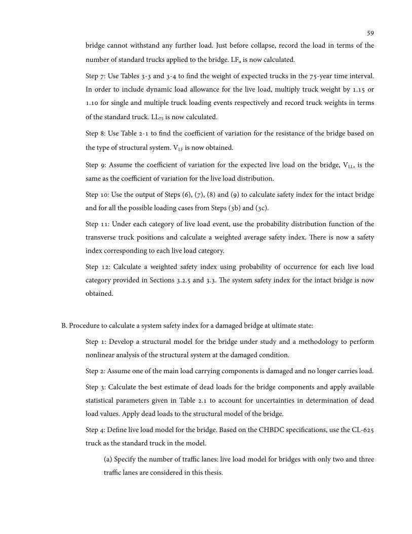
bridge cannot withstand any further load. Just before collapse, record the load in terms of the
number of standard trucks applied to the bridge. LFu is now calculated.
Step : Use Tables - and - to 'nd the weight of expected trucks in the -year time interval.
In order to include dynamic load allowance for the live load, multiply truck weight by . or
. for single and multiple truck loading events respectively and record truck weights in terms
of the standard truck. LL75 is now calculated.
Step : Use Table - to 'nd the coefficient of variation for the resistance of the bridge based on
the type of structural system. VLF is now obtained.
Step : Assume the coefficient of variation for the expected live load on the bridge, VLL, is the
same as the coefficient of variation for the live load distribution.
Step : Use the output of Steps (), (), () and () to calculate safety index for the intact bridge
and for all the possible loading cases from Steps (b) and (c).
Step : Under each category of live load event, use the probability distribution function of the
transverse truck positions and calculate a weighted average safety index. ere is now a safety
index corresponding to each live load category.
Step : Calculate a weighted safety index using probability of occurrence for each live load
category provided in Sections .. and .. e system safety index for the intact bridge is now
obtained.
B. Procedure to calculate a system safety index for a damaged bridge at ultimate state:
Step : Develop a structural model for the bridge under study and a methodology to perform
nonlinear analysis of the structural system at the damaged condition.
Step : Assume one of the main load carrying components is damaged and no longer carries load.
Step : Calculate the best estimate of dead loads for the bridge components and apply available
statistical parameters given in Table . to account for uncertainties in determination of dead
load values. Apply dead loads to the structural model of the bridge.
Step : De'ne live load model for the bridge. Based on the CHBDC speci'cations, use the CL-
truck as the standard truck in the model.
(a) Specify the number of traffic lanes: live load model for bridges with only two and three
traffic lanes are considered in this thesis.

(b) Determine possible loading events (single and multiple side-by-side trucks). For the
case of adjacent trucks consider three correlation factors (ρ=., . and .), when
required statistics are available.
(c) Consider multiple transverse positions for the trucks in the traffic lanes. Figure -
provides the probability distribution function for transverse position of the trucks. For a
more systematic analysis, develop categories for possible live load events (single-truck,
double-truck with ρ=., double-truck with ρ=. and double-truck with ρ=., etc.) and
list different truck transverse positions under each category.
Step : Identify a longitudinal loading position that creates the maximum effect at a critical
location, e.g. mid-span.
Step : Apply live loads to the structural model of the bridge. Live load cases should include all
truck con'gurations de'ned in Steps (b), (c) and (). In all load cases, weight of the primary
truck at initial condition is equivalent to the weight of the standard truck (in this case kN).
Step : Increase live load incrementally and perform nonlinear structural analysis of the damaged
structural system. Continue increasing load until the bridge cannot withstand any further load.
Just before collapse, record the load in terms of the number of standard trucks applied to the
bridge. LFd is now calculated.
Step : Use Tables . and . to 'nd weight of the expected trucks in years, year, months,
months, month, weeks and day. In order to include dynamic load allowance for live load,
multiply truck weight by . or . for single and multiple truck loading events respectively
and record truck weights in terms of the standard truck. LLE is now calculated for various
exposure times.
Step : Based on the performed structural analysis, obtain load-de1ection response of the bridge
at both intact and damaged conditions.
Step : Calculate de1ection limits provided in Section . and determine visible de1ections for
the public.
Step : Use outputs of Steps (), () and () to determine the load at which de1ections become
visible to the public. Determine the exposure time that the expected load would reach such a level
and mark it as the damaged detection time. If load-de1ection response of the bridge
indicates that the de1ection of the damaged bridge at ultimate is not noticeable, time interval of
years will be taken as damage detection time. e minimum of damaged detection
time should not be smaller than months for all loading cases.
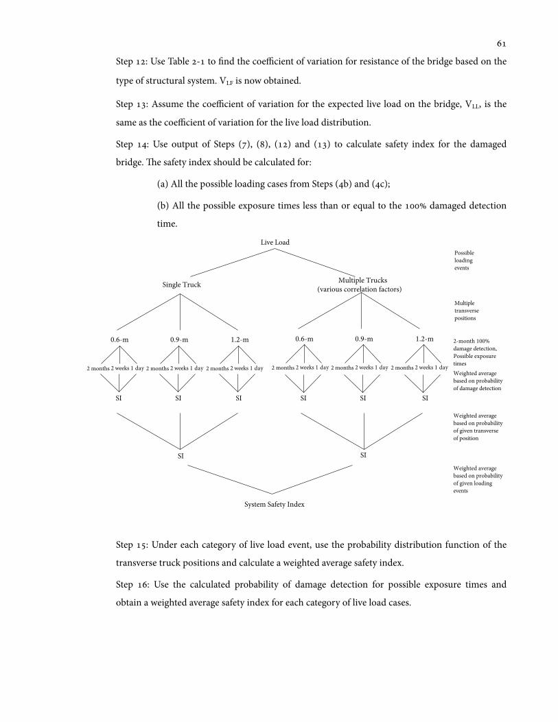
Step : Use Table - to 'nd the coefficient of variation for resistance of the bridge based on the
type of structural system. VLF is now obtained.
Step : Assume the coefficient of variation for the expected live load on the bridge, VLL, is the
same as the coefficient of variation for the live load distribution.
Step : Use output of Steps (), (), () and () to calculate safety index for the damaged
bridge. e safety index should be calculated for:
(a) All the possible loading cases from Steps (b) and (c);
(b) All the possible exposure times less than or equal to the damaged detection
time.
Step : Under each category of live load event, use the probability distribution function of the
transverse truck positions and calculate a weighted average safety index.
Step : Use the calculated probability of damage detection for possible exposure times and
obtain a weighted average safety index for each category of live load cases.
2 months 2 weeks 1 day
0.6-m 0.9-m 1.2-m 2-month 100% damage detection, Possible exposure times
2 months 2 weeks 1 day 2 months 2 weeks 1 day 2 months 2 weeks 1 day
0.6-m 0.9-m 1.2-m
2 months 2 weeks 1 day 2 months 2 weeks 1 day
Single Truck Multiple Trucks (various correlation factors)
Multiple transverse positions
Live LoadPossible loading events
SI
System Safety Index
Weighted average based on probability of damage detection
Weighted average based on probability of given transverse of position
Weighted average based on probability of given loading events
SI SI SI SI SI
SISI

Step : Calculate a weighted safety index using probability of occurrence for each live load
category provided in Sections .. and .. e system safety index for the damaged bridge is
now obtained.
Step : Repeat the procedure for all possible critical members in damaged condition and select
the lowest safety index for the structural system.
Use the Standard Normal Distribution Table to convert the system safety index values to the
corresponding failure probability values. If values of the failure probability at the ultimate for intact and
damaged conditions are less than ⁶ and .x1 respectively, the bridge is considered to be redundant
and safe.
Given the step-by-step formulation, two 1owcharts are prepared and provided in the next Section to
summarize the procedure of assessing reliability of bridges with two lanes of traffic at the system level.
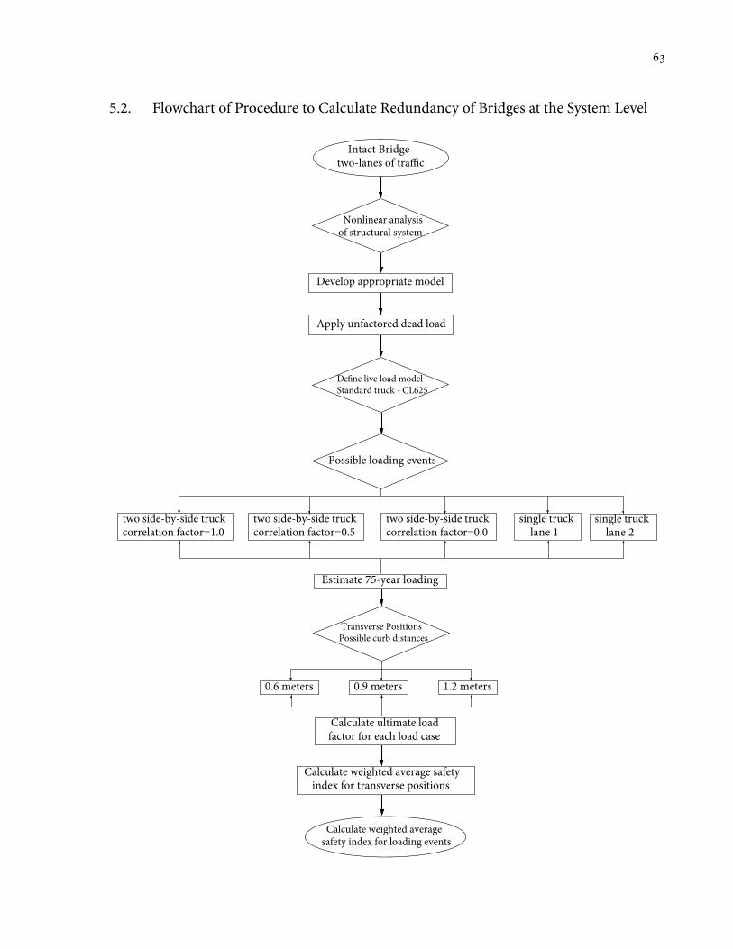
5.2. Flowchart of Procedure to Calculate Redundancy of Bridges at the System Level
Intact Bridgetwo-lanes of tra!c
Nonlinear analysis of structural system
Develop appropriate model
Apply unfactored dead load
De"ne live load modelStandard truck - CL625
Estimate 75-year loading
Possible loading events
two side-by-side truck correlation factor=1.0
two side-by-side truck correlation factor=0.5
two side-by-side truck correlation factor=0.0
single truck lane 1
single truck lane 2
Transverse Positions Possible curb distances
0.6 meters 0.9 meters 1.2 meters
Calculate ultimate load factor for each load case
Calculate weighted average safety index for transverse positions
Calculate weighted average safety index for loading events
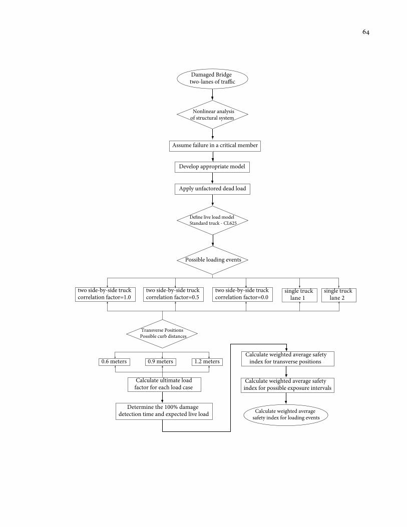
Damaged Bridgetwo-lanes of tra!c
Nonlinear analysis of structural system
Develop appropriate model
Apply unfactored dead load
De"ne live load modelStandard truck - CL625
Determine the 100% damage detection time and expected live load
Possible loading events
two side-by-side truck correlation factor=1.0
two side-by-side truck correlation factor=0.5
two side-by-side truck correlation factor=0.0
single truck lane 1
single truck lane 2
Transverse Positions Possible curb distances
0.6 meters 0.9 meters 1.2 meters
Calculate ultimate load factor for each load case
Calculate weighted average safety index for transverse positions
Calculate weighted average safety index for loading events
Assume failure in a critical member
Calculate weighted average safety index for possible exposure intervals

Chapter 6
e Montreal River Bridge Concept - a Twin Steel Girder Bridge
In this chapter, the previously developed guidelines are used to study redundancy of a two-girder steel
bridge at the system level. is is an attempt to show that efficient two-girder bridges should not
necessarily be classi'ed as non-redundant structures. In general, redundancy is interpreted to be the
result of having more than one primary load path (load-path redundancy), while the static indeterminacy
in continuous structures can be used to create adequate level of redundancy. erefore, behavior of the
three-span Montreal River Bridge concept before and aer failure of a critical member is studied and the
level of redundancy is calculated. It is assumed that a truck has hit the bridge from below and the bottom
1ange of one girder at mid-span is damaged. High impacts and extreme cold temperatures or possible
1aws in the steel cross section could also be factors damaging the bridge. As part of safety index
calculations, nonlinear analysis of the bridge, at both intact and damaged conditions, is performed and
behavior of the structure at the ultimate state is explained.
e following topics will be addressed in this chapter:
() Brief description of the Montreal River Bridge Concept;
() Structural behavior of the Montreal River Bridge Concept;

() Grillage model of the bridge to perform nonlinear analysis of the structure;
() e ultimate capacity of the bridge at intact and damaged conditions;
() Calculation of System Safety Indices for the bridge;
() Redundancy of the bridge.
6.1. Brief Description of the Montreal River Bridge
e Montreal River Bridge was designed by Kris Mermigas and constructed over the Montreal River in
Matachewan, Ontario. e bridge consists of four continuous haunched steel I-girders over three spans
(, and meters). In a recent study by Kris Mermigas, the bridge was redesigned with twin girders
to perform a cost comparison between the two alternative designs (Mermigas, ). Although the twin
girder concept was never built, it was designed according to the Canadian Highway Bridge Design Code
and complies with all the code requirements (Mermigas, ). is chapter studies the redundancy level
of the twin girder bridge concept. e structural system of the Montreal River Bridge concept (from this
point on, the Montreal River Bridge) includes two continuous haunched steel I-girders composite with a
mm concrete deck. e bridge has two traffic lanes with shoulders on both sides, a sidewalk on the
south side and parapet walls resulting in a total width of . meters as shown in Figure -.
(a) Plan
(b) Elevation

(c) Cross section
Figure 6-1: e Montreal River Bridge Concept (Drawn by Kris Mermigas)
Material properties for the Montreal River Bridge are summarized in Table -. All structural steel
conforms to the CAN/CSA G-./G.- with Grade AT category or Grade A. Concrete
with a compressive strength of MPa and Grade reinforcing steel is used for the deck.
Material Strength Modulus of ElasticityConcrete (Deck) Speci'ed compressive strength:
′fc = 30 MPaEc = 25000MPa
Reinforcing Steel (Grade ) Yield strength:fy = 400MPa
Es = 200000 MPa
Structural Steel (Grade AT) Yield strength:
Ultimate Strength
fy = 350 MPa
fu = 480 MPa
Es = 200000 MPa
Table 6-1: Material properties for the Montreal River Bridge
6.2. Structural Behavior - Intact Bridge
Simple formulation of the limit state function is not generally possible; therefore, performance of a
structural member is typically de'ned by a series of limit state functions. Bending moment capacity, shear
capacity, overall or local buckling capacity and material deterioration should be examined for a typical
girder bridge. Factors that in1uence the bridge user’s level of comfort such as maximum de1ections and
vibration need to be checked. (Nowak and Zhou, )
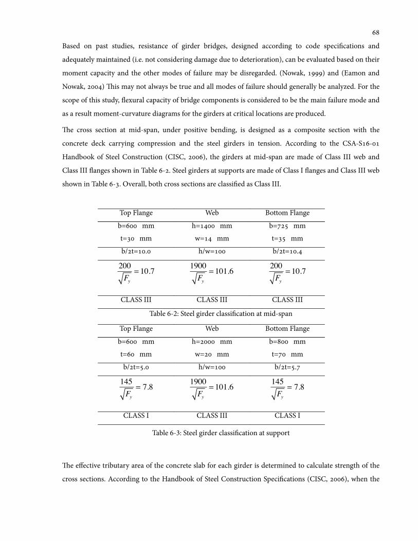
Based on past studies, resistance of girder bridges, designed according to code speci'cations and
adequately maintained (i.e. not considering damage due to deterioration), can be evaluated based on their
moment capacity and the other modes of failure may be disregarded. (Nowak, ) and (Eamon and
Nowak, ) is may not always be true and all modes of failure should generally be analyzed. For the
scope of this study, 1exural capacity of bridge components is considered to be the main failure mode and
as a result moment-curvature diagrams for the girders at critical locations are produced.
e cross section at mid-span, under positive bending, is designed as a composite section with the
concrete deck carrying compression and the steel girders in tension. According to the CSA-S-
Handbook of Steel Construction (CISC, ), the girders at mid-span are made of Class III web and
Class III 1anges shown in Table -. Steel girders at supports are made of Class I 1anges and Class III web
shown in Table -. Overall, both cross sections are classi'ed as Class III.
Top Flange Web Bottom Flange
b= mm h= mm b= mm
t= mm w= mm t= mm
b/t=. h/w= b/t=.
200Fy
= 10.7 1900Fy
= 101.6 200Fy
= 10.7
CLASS III CLASS III CLASS III
Table 6-2: Steel girder classi'cation at mid-span
Top Flange Web Bottom Flange
b= mm h= mm b= mm
t= mm w= mm t= mm
b/t=. h/w= b/t=.
145Fy
= 7.8 1900Fy
= 101.6 145Fy
= 7.8
CLASS I CLASS III CLASS I
Table 6-3: Steel girder classi'cation at support
e effective tributary area of the concrete slab for each girder is determined to calculate strength of the
cross sections. According to the Handbook of Steel Construction Speci'cations (CISC, ), when the

slab extends on both sides of the steel girder, effective slab width is the lesser of one-fourth of the girder
span and centre-to-centre distance of the steel girders.
e ultimate capacity of the Montreal River Bridge at mid-span is calculated based on the complete
composite action between girders and the concrete slab. e deck slab has a thickness of mm and an
effective width of mm. Analysis of the cross section at mid-span shows that the bottom 1ange of the
girder at failure starts to yield in tension, followed by concrete crushing. Aer the concrete crushes, the
steel girder carries load with the top 1ange in compression. e crushed concrete deck is no longer
effective to support compression 1ange of the steel girder; therefore, local buckling of the compression
1ange can be expected as soon as the Class III section yields in compression. At this stage, the cross
section has limited capacity and ductility and can be assumed that its capacity drops to zero. e
moment-curvature diagram of the cross section at mid-span is shown in Figure -.
Figure 6-2: Moment-Curvature diagram at mid-span and supports
e cross section at pier locations takes negative moment with concrete deck in tension. e unsupported
bottom 1ange of the I-girder is in compression with possible loss of stability due to local and lateral
torsional buckling. Effectiveness of the concrete slab in tension is ignored but the reinforcement in
effective slab width contributes to moment resistance of the section. As already stated, the steel girder is
made of Class I 1anges and Class III web. Based on Laane and Lebet () class of 1ange section mainly
determines behavior of the cross section, while according to Eurocode : Design of Steel Structures (CEN,
) cross sections with Class III web and Class I or II 1anges are treated as effective Class II cross
sections. erefore, it can be expected that the section capacity at supports exceeds that of a typical class
III section.
Bottom !ange yields in tension
Concrete crushes
Bottom !ange yields in compression
0
5000
10000
15000
20000
25000
30000
35000
40000
45000
50000
0.0E+00 5.0E-06 1.0E-05 1.5E-05 2.0E-05 2.5E-05
Mom
ent (
kN.m
)
Curvature (rad/mm)
Mid-Span Support-Code Support - Laane & Lebet Model
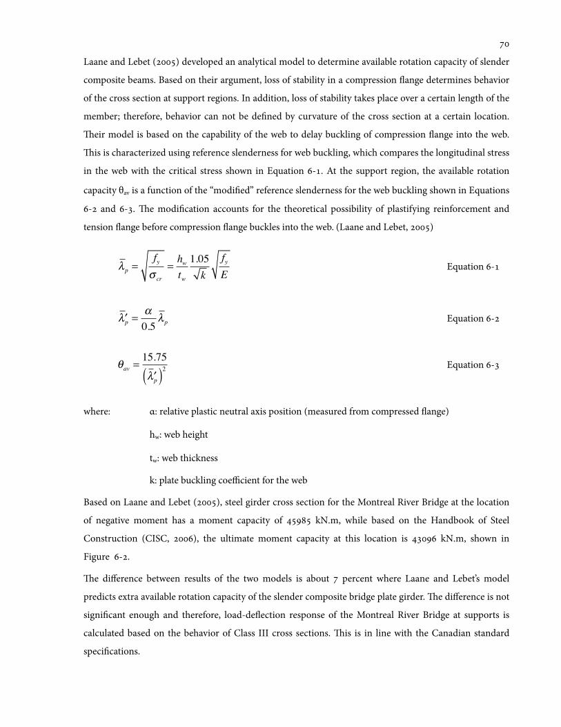
Laane and Lebet () developed an analytical model to determine available rotation capacity of slender
composite beams. Based on their argument, loss of stability in a compression 1ange determines behavior
of the cross section at support regions. In addition, loss of stability takes place over a certain length of the
member; therefore, behavior can not be de'ned by curvature of the cross section at a certain location.
eir model is based on the capability of the web to delay buckling of compression 1ange into the web.
is is characterized using reference slenderness for web buckling, which compares the longitudinal stress
in the web with the critical stress shown in Equation -. At the support region, the available rotation
capacity θav is a function of the “modi'ed” reference slenderness for the web buckling shown in Equations
- and -. e modi'cation accounts for the theoretical possibility of plastifying reinforcement and
tension 1ange before compression 1ange buckles into the web. (Laane and Lebet, )
λp =fyσ cr
=hwtw
1.05k
fyE
Equation -
′λp =α0.5
λp Equation -
θav =15.75
′λp( )2Equation -
where: α: relative plastic neutral axis position (measured from compressed 1ange)
hw: web height
tw: web thickness
k: plate buckling coefficient for the web
Based on Laane and Lebet (), steel girder cross section for the Montreal River Bridge at the location
of negative moment has a moment capacity of kN.m, while based on the Handbook of Steel
Construction (CISC, ), the ultimate moment capacity at this location is kN.m, shown in
Figure -.
e difference between results of the two models is about percent where Laane and Lebet’s model
predicts extra available rotation capacity of the slender composite bridge plate girder. e difference is not
signi'cant enough and therefore, load-de1ection response of the Montreal River Bridge at supports is
calculated based on the behavior of Class III cross sections. is is in line with the Canadian standard
speci'cations.
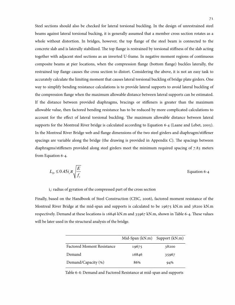
Steel sections should also be checked for lateral torsional buckling. In the design of unrestrained steel
beams against lateral torsional bucking, it is generally assumed that a member cross section rotates as a
whole without distortion. In bridges, however, the top 1ange of the steel beam is connected to the
concrete slab and is laterally stabilized. e top 1ange is restrained by torsional stiffness of the slab acting
together with adjacent steel sections as an inverted U-frame. In negative moment regions of continuous
composite beams at pier locations, when the compression 1ange (bottom 1ange) buckles laterally, the
restrained top 1ange causes the cross section to distort. Considering the above, it is not an easy task to
accurately calculate the limiting moment that causes lateral torsional buckling of bridge plate girders. One
way to simplify bending resistance calculations is to provide lateral supports to avoid lateral buckling of
the compression 1ange when the maximum allowable distance between lateral supports can be estimated.
If the distance between provided diaphragms, bracings or stiffeners is greater than the maximum
allowable value, then factored bending resistance has to be reduced by more complicated calculations to
account for the effect of lateral torsional buckling. e maximum allowable distance between lateral
supports for the Montreal River bridge is calculated according to Equation - (Laane and Lebet, ).
In the Montreal River Bridge web and 1ange dimensions of the two steel girders and diaphragm/stiffener
spacings are variable along the bridge (the drawing is provided in Appendix C). e spacings between
diaphragms/stiffeners provided along steel girders meet the minimum required spacing of . meters
from Equation -.
LD ≤ 0.45icπEfy
Equation -
ic: radius of gyration of the compressed part of the cross section
Finally, based on the Handbook of Steel Construction (CISC, ), factored moment resistance of the
Montreal River Bridge at the mid-span and supports is calculated to be kN.m and kN.m
respectively. Demand at these locations is kN.m and kN.m, shown in Table -. ese values
will be later used in the structural analysis of the bridge.
Mid-Span (kN.m) Support (kN.m)
Factored Moment Resistance
Demand
Demand/Capacity ()
Table 6-4: Demand and Factored Resistance at mid-span and supports

6.3. Grillage Model
6.3.1. Intact Bridge
e 'rst step to perform reliability analysis of a bridge is to establish an accurate deterministic structural
model; probabilistic aspects can then be included. e Montreal River Bridge has two degrees of
indeterminacy including load distribution in the transverse direction. In current literature, to capture
behavior of a bridge under various load cases for reliability analysis, generally a D 'nite element model
is utilized to analyze the structure. is increases complexity of analysis and engineers in practice may not
adapt this procedure to check safety in the design of new bridges. It should be noted that an accurate D
model can provide valuable information on the behavior of bridges under traffic loads. For example in the
case of Montreal River Bridge, it can be assumed that under symmetric loading (two side-by-side trucks),
each girder takes half of the applied load in the transverse direction. e assumption reduces degree of
indeterminacy to one and a preliminary accurate D model may be employed to evaluate behavior of the
bridge under expected traffic loads.
For the purpose of this thesis, SAP is used to generate a D nonlinear grillage model for the
Montreal River Bridge shown in Figure -, and the composite girders are modeled as two equivalent
beams. In grillage modeling, bridge structures can be idealized as a grid of longitudinal and transverse
beams with speci'ed bending and torsional stiffness. De1ection and slope compatibility at transverse and
longitudinal beam joints are utilized to solve the model under applied loads (O'Brien and Keogh, ).
Membrane action and slab arching are ignored, but the grillage model generally provides a relatively
accurate behavior of the bridge and distribution of loads in the main members(O'Brien and Keogh, ).
Figure 6-3: Grillage model for the Montreal River Bridge

In the grillage model of the Montreal River Bridge, two longitudinal beams are used to model the two
steel girders and the effective concrete slab that contributes to bending and torsional stiffness of the
bridge longitudinally. Moment of Inertia (I) and torsional constant (J) for the concrete deck are calculated
based on an equivalent transformed steel section and incorporated in the model by application of
modi'cation factors for the longitudinal member properties.
In addition, transverse beams are used to model the deck slab with a transverse member spacing of
mm in the side spans. In the central span, uniform but closer spacing of mm is utilized to increase
accuracy of the grillage analysis where truck loads will later be applied. e moment of inertia and the
torsional constant for longitudinal and transverse sections are speci'ed based on the uncracked
properties of the bridge cross section.
6.3.2. Damaged Bridge
Based on the developed procedure to calculate redundancy, it is necessary to study the behavior of
bridges aer failure of a critical component (Section .). In the case of the Montreal River Bridge, it is
assumed that the bottom 1ange of steel girder at mid-span is hit by a truck from below. High impacts and
extreme cold temperatures or possible 1aws in the steel cross section could also be factors damaging the
bridge. Failure of the tension 1ange results in the loss of moment carrying capacity at mid-span. To be
conservative, it is also assumed that the cross section is no longer capable of transferring shear.
e two steel girders are symmetrically positioned with regard to center line of the cross section, but live
load is not evenly distributed between the two girders due to the presence of a side-walk on the south side
of the bridge. Given that the fast traffic lane is located on the north side and that the probability of having
heavy traffic on the south side is larger, the girder on the south side is more critical. Transverse
distribution of live load will be discussed in more detail in Section ..
e SAP intact grillage model is modi'ed to account for the damage at mid-span of the south girder.
In doing so, moment and shear transfer are both released at a de'ned speci'c joint at mid-span of the
south girder, implying that the cross section has no moment or shear capacity. e rest of the model is
similar to that of the intact bridge.
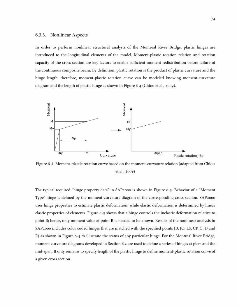
6.3.3. Nonlinear Aspects
In order to perform nonlinear structural analysis of the Montreal River Bridge, plastic hinges are
introduced to the longitudinal elements of the model. Moment-plastic rotation relation and rotation
capacity of the cross section are key factors to enable sufficient moment redistribution before failure of
the continuous composite beam. By de'nition, plastic rotation is the product of plastic curvature and the
hinge length; therefore, moment-plastic rotation curve can be modeled knowing moment-curvature
diagram and the length of plastic hinge as shown in Figure - (Chiou et al., ).
Figure 6-4: Moment-plastic rotation curve based on the moment-curvature relation (adapted from Chiou
et al., 2009)
e typical required “hinge property data” in SAP is shown in Figure -. Behavior of a “Moment
Type” hinge is de'ned by the moment-curvature diagram of the corresponding cross section. SAP
uses hinge properties to estimate plastic deformation, while elastic deformation is determined by linear
elastic properties of elements. Figure - shows that a hinge controls the inelastic deformation relative to
point B; hence, only moment value at point B is needed to be known. Results of the nonlinear analysis in
SAP includes color coded hinges that are matched with the speci'ed points (B, IO, LS, CP, C, D and
E) as shown in Figure - to illustrate the status of any particular hinge. For the Montreal River Bridge,
moment curvature diagrams developed in Section . are used to de'ne a series of hinges at piers and the
mid-span. It only remains to specify length of the plastic hinge to de'ne moment-plastic rotation curve of
a given cross section.
Mom
ent
Curvature Plastic rotation, !p
Mom
ent
"pLp
M
My
M
My
"y "
"p
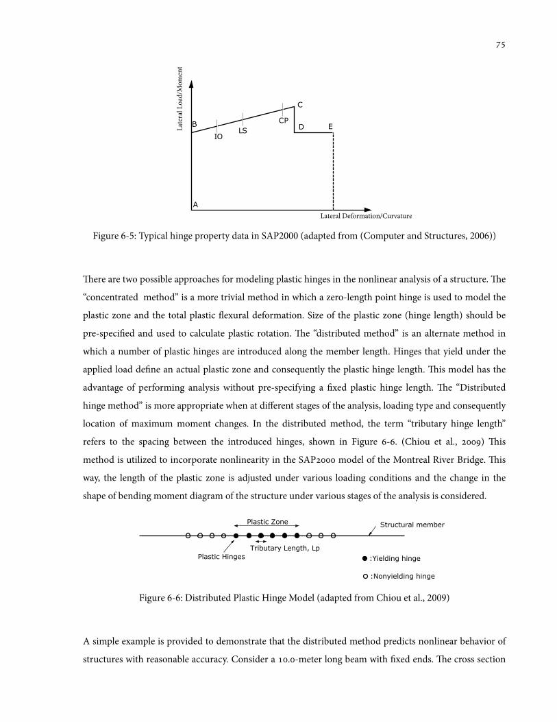
Figure 6-5: Typical hinge property data in SAP2000 (adapted from (Computer and Structures, 2006))
ere are two possible approaches for modeling plastic hinges in the nonlinear analysis of a structure. e
“concentrated method” is a more trivial method in which a zero-length point hinge is used to model the
plastic zone and the total plastic 1exural deformation. Size of the plastic zone (hinge length) should be
pre-speci'ed and used to calculate plastic rotation. e “distributed method” is an alternate method in
which a number of plastic hinges are introduced along the member length. Hinges that yield under the
applied load de'ne an actual plastic zone and consequently the plastic hinge length. is model has the
advantage of performing analysis without pre-specifying a 'xed plastic hinge length. e “Distributed
hinge method” is more appropriate when at different stages of the analysis, loading type and consequently
location of maximum moment changes. In the distributed method, the term “tributary hinge length”
refers to the spacing between the introduced hinges, shown in Figure -. (Chiou et al., ) is
method is utilized to incorporate nonlinearity in the SAP model of the Montreal River Bridge. is
way, the length of the plastic zone is adjusted under various loading conditions and the change in the
shape of bending moment diagram of the structure under various stages of the analysis is considered.
Figure 6-6: Distributed Plastic Hinge Model (adapted from Chiou et al., 2009)
A simple example is provided to demonstrate that the distributed method predicts nonlinear behavior of
structures with reasonable accuracy. Consider a .-meter long beam with 'xed ends. e cross section
A
B
IOLS
CP
C
D ELate
ral L
oad/
Mom
ent
Lateral Deformation/Curvature
Plastic Zone
Tributary Length, Lp
Plastic Hinges
Structural member
:Yielding hinge
:Nonyielding hinge
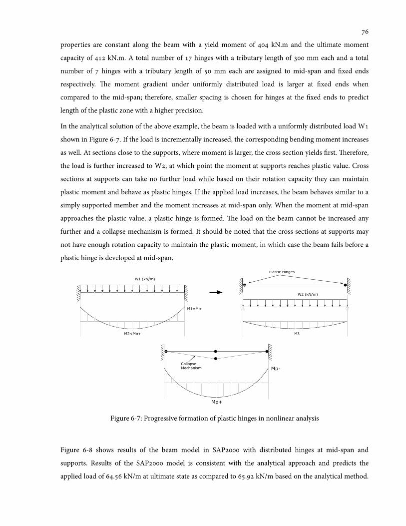
properties are constant along the beam with a yield moment of kN.m and the ultimate moment
capacity of kN.m. A total number of hinges with a tributary length of mm each and a total
number of hinges with a tributary length of mm each are assigned to mid-span and 'xed ends
respectively. e moment gradient under uniformly distributed load is larger at 'xed ends when
compared to the mid-span; therefore, smaller spacing is chosen for hinges at the 'xed ends to predict
length of the plastic zone with a higher precision.
In the analytical solution of the above example, the beam is loaded with a uniformly distributed load W
shown in Figure -. If the load is incrementally increased, the corresponding bending moment increases
as well. At sections close to the supports, where moment is larger, the cross section yields 'rst. erefore,
the load is further increased to W, at which point the moment at supports reaches plastic value. Cross
sections at supports can take no further load while based on their rotation capacity they can maintain
plastic moment and behave as plastic hinges. If the applied load increases, the beam behaves similar to a
simply supported member and the moment increases at mid-span only. When the moment at mid-span
approaches the plastic value, a plastic hinge is formed. e load on the beam cannot be increased any
further and a collapse mechanism is formed. It should be noted that the cross sections at supports may
not have enough rotation capacity to maintain the plastic moment, in which case the beam fails before a
plastic hinge is developed at mid-span.
Figure 6-7: Progressive formation of plastic hinges in nonlinear analysis
Figure - shows results of the beam model in SAP with distributed hinges at mid-span and
supports. Results of the SAP model is consistent with the analytical approach and predicts the
applied load of . kN/m at ultimate state as compared to . kN/m based on the analytical method.
W1 (kN/m)
M1=Mp-
M2<Mp+ M3
Mp+
Mp-
W2 (kN/m)
Collapse Mechanism
Plastic Hinges
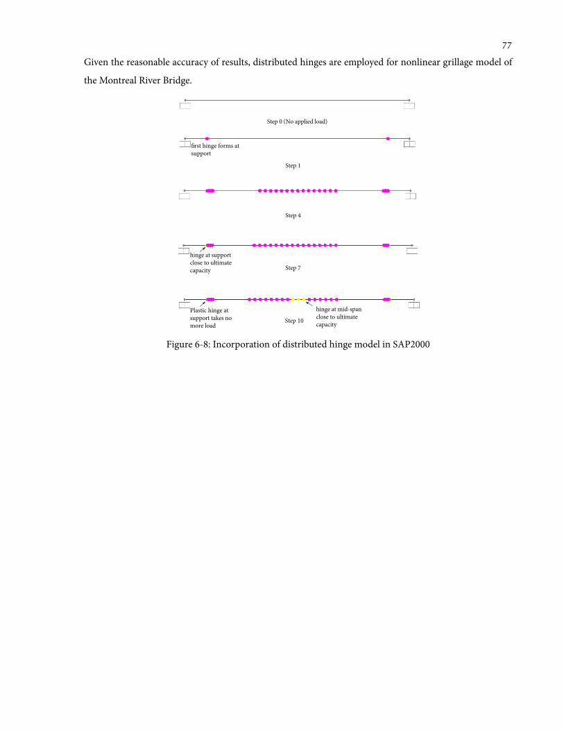
Given the reasonable accuracy of results, distributed hinges are employed for nonlinear grillage model of
the Montreal River Bridge.
Figure 6-8: Incorporation of distributed hinge model in SAP2000
Step 0 (No applied load)
Step 1
Step 4
Step 7
Step 10
hinge at support close to ultimate capacity
Plastic hinge at support takes no more load
hinge at mid-span close to ultimate capacity
!rst hinge forms at support
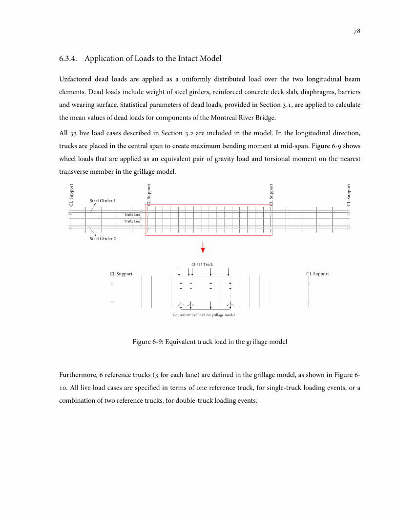
6.3.4. Application of Loads to the Intact Model
Unfactored dead loads are applied as a uniformly distributed load over the two longitudinal beam
elements. Dead loads include weight of steel girders, reinforced concrete deck slab, diaphragms, barriers
and wearing surface. Statistical parameters of dead loads, provided in Section ., are applied to calculate
the mean values of dead loads for components of the Montreal River Bridge.
All live load cases described in Section . are included in the model. In the longitudinal direction,
trucks are placed in the central span to create maximum bending moment at mid-span. Figure - shows
wheel loads that are applied as an equivalent pair of gravity load and torsional moment on the nearest
transverse member in the grillage model.
Figure 6-9: Equivalent truck load in the grillage model
Furthermore, reference trucks ( for each lane) are de'ned in the grillage model, as shown in Figure -
. All live load cases are speci'ed in terms of one reference truck, for single-truck loading events, or a
combination of two reference trucks, for double-truck loading events.
CL S
uppo
rt
CL S
uppo
rt
CL S
uppo
rt
CL S
uppo
rt
Tra!c Lane
Tra!c Lane
Steel Girder 1
Steel Girder 2
CL Support
Cl-625 Truck
Equivalent live load on grillage model
CL Support
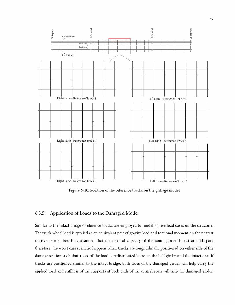
Figure 6-10: Position of the reference trucks on the grillage model
6.3.5. Application of Loads to the Damaged Model
Similar to the intact bridge reference trucks are employed to model live load cases on the structure.
e truck wheel load is applied as an equivalent pair of gravity load and torsional moment on the nearest
transverse member. It is assumed that the 1exural capacity of the south girder is lost at mid-span;
therefore, the worst case scenario happens when trucks are longitudinally positioned on either side of the
damage section such that of the load is redistributed between the half girder and the intact one. If
trucks are positioned similar to the intact bridge, both sides of the damaged girder will help carry the
applied load and stiffness of the supports at both ends of the central span will help the damaged girder.
CL S
uppo
rt
CL S
uppo
rt
CL S
uppo
rt
CL S
uppo
rt
Right Lane - Reference Truck 1
Right Lane - Reference Truck 2
Right Lane - Reference Truck 3
Le! Lane - Reference Truck 4
Le! Lane - Reference Truck 5
Le! Lane - Reference Truck 6
Tra"c Lane
Tra"c Lane
North Girder
South Girder
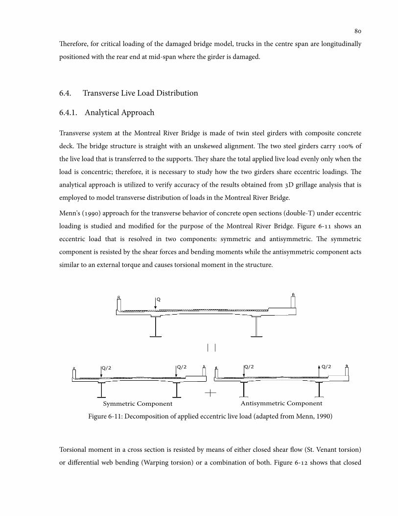
erefore, for critical loading of the damaged bridge model, trucks in the centre span are longitudinally
positioned with the rear end at mid-span where the girder is damaged.
6.4. Transverse Live Load Distribution
6.4.1. Analytical Approach
Transverse system at the Montreal River Bridge is made of twin steel girders with composite concrete
deck. e bridge structure is straight with an unskewed alignment. e two steel girders carry of
the live load that is transferred to the supports. ey share the total applied live load evenly only when the
load is concentric; therefore, it is necessary to study how the two girders share eccentric loadings. e
analytical approach is utilized to verify accuracy of the results obtained from D grillage analysis that is
employed to model transverse distribution of loads in the Montreal River Bridge.
Menn's () approach for the transverse behavior of concrete open sections (double-T) under eccentric
loading is studied and modi'ed for the purpose of the Montreal River Bridge. Figure - shows an
eccentric load that is resolved in two components: symmetric and antisymmetric. e symmetric
component is resisted by the shear forces and bending moments while the antisymmetric component acts
similar to an external torque and causes torsional moment in the structure.
Figure 6-11: Decomposition of applied eccentric live load (adapted from Menn, 1990)
Torsional moment in a cross section is resisted by means of either closed shear 1ow (St. Venant torsion)
or differential web bending (Warping torsion) or a combination of both. Figure - shows that closed
Q
Q/2Q/2Q/2 Q/2
Antisymmetric ComponentSymmetric Component
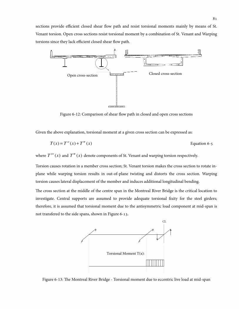
sections provide efficient closed shear 1ow path and resist torsional moments mainly by means of St.
Venant torsion. Open cross sections resist torsional moment by a combination of St. Venant and Warping
torsions since they lack efficient closed shear 1ow path.
Figure 6-12: Comparison of shear 1ow path in closed and open cross sections
Given the above explanation, torsional moment at a given cross section can be expressed as:
T (x) = T sv (x) + TW (x) Equation -
where T SV (x) and TW (x) denote components of St. Venant and warping torsion respectively.
Torsion causes rotation in a member cross section; St. Venant torsion makes the cross section to rotate in-
plane while warping torsion results in out-of-plane twisting and distorts the cross section. Warping
torsion causes lateral displacement of the member and induces additional longitudinal bending.
e cross section at the middle of the centre span in the Montreal River Bridge is the critical location to
investigate. Central supports are assumed to provide adequate torsional 'xity for the steel girders;
therefore, it is assumed that torsional moment due to the antisymmetric load component at mid-span is
not transfered to the side spans, shown in Figure -.
Figure 6-13: e Montreal River Bridge - Torsional moment due to eccentric live load at mid-span
Closed cross-sectionOpen cross-section
CL
Torsional Moment T(x):
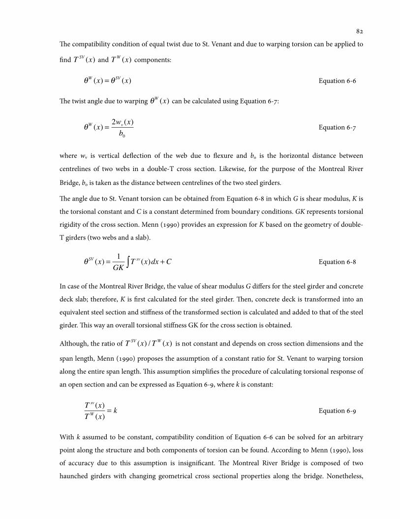
e compatibility condition of equal twist due to St. Venant and due to warping torsion can be applied to
'nd T SV (x) and TW (x) components:
θW (x) = θ SV (x) Equation -
e twist angle due to warping θW (x) can be calculated using Equation -:
θW (x) = 2wv (x)b0
Equation -
where wv is vertical de1ection of the web due to 1exure and bo is the horizontal distance between
centrelines of two webs in a double-T cross section. Likewise, for the purpose of the Montreal River
Bridge, bo is taken as the distance between centrelines of the two steel girders.
e angle due to St. Venant torsion can be obtained from Equation - in which G is shear modulus, K is
the torsional constant and C is a constant determined from boundary conditions. GK represents torsional
rigidity of the cross section. Menn () provides an expression for K based on the geometry of double-
T girders (two webs and a slab).
θ SV (x) = 1GK
T sv (x)dx + C∫ Equation -
In case of the Montreal River Bridge, the value of shear modulus G differs for the steel girder and concrete
deck slab; therefore, K is 'rst calculated for the steel girder. en, concrete deck is transformed into an
equivalent steel section and stiffness of the transformed section is calculated and added to that of the steel
girder. is way an overall torsional stiffness GK for the cross section is obtained.
Although, the ratio of T SV (x) /TW (x) is not constant and depends on cross section dimensions and the
span length, Menn () proposes the assumption of a constant ratio for St. Venant to warping torsion
along the entire span length. is assumption simpli'es the procedure of calculating torsional response of
an open section and can be expressed as Equation -, where k is constant:
T sv (x)TW (x)
= k Equation -
With k assumed to be constant, compatibility condition of Equation - can be solved for an arbitrary
point along the structure and both components of torsion can be found. According to Menn (), loss
of accuracy due to this assumption is insigni'cant. e Montreal River Bridge is composed of two
haunched girders with changing geometrical cross sectional properties along the bridge. Nonetheless,
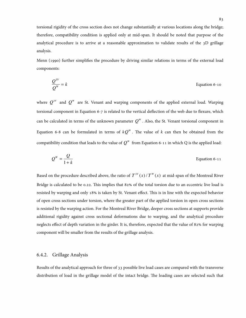
torsional rigidity of the cross section does not change substantially at various locations along the bridge;
therefore, compatibility condition is applied only at mid-span. It should be noted that purpose of the
analytical procedure is to arrive at a reasonable approximation to validate results of the D grillage
analysis.
Menn () further simpli'es the procedure by driving similar relations in terms of the external load
components:
QSV
QW = k Equation -
where QSV and QW are St. Venant and warping components of the applied external load. Warping
torsional component in Equation - is related to the vertical de1ection of the web due to 1exure, which
can be calculated in terms of the unknown parameter QW . Also, the St. Venant torsional component in
Equation - can be formulated in terms of kQW . e value of k can then be obtained from the
compatibility condition that leads to the value of QW from Equation - in which Q is the applied load:
QW =Q1+ k
Equation -
Based on the procedure described above, the ratio of T SV (x) /TW (x) at mid-span of the Montreal River
Bridge is calculated to be .. is implies that of the total torsion due to an eccentric live load is
resisted by warping and only is taken by St. Venant effect. is is in line with the expected behavior
of open cross sections under torsion, where the greater part of the applied torsion in open cross sections
is resisted by the warping action. For the Montreal River Bridge, deeper cross sections at supports provide
additional rigidity against cross sectional deformations due to warping, and the analytical procedure
neglects effect of depth variation in the girder. It is, therefore, expected that the value of for warping
component will be smaller from the results of the grillage analysis.
6.4.2. Grillage Analysis
Results of the analytical approach for three of possible live load cases are compared with the transverse
distribution of load in the grillage model of the intact bridge. e loading cases are selected such that

typical positions of trucks in the transverse direction are covered and results can be expanded to all the
cases. e selected load cases are:
. Two trucks side-by-side with correlation factor of . and curb distance of . meters;
. One truck in the right lane with curb distance of . meters;
. One truck in the le lane with curb distance of . meters.
Table - summarizes moment values from the grillage analysis for both girders at the mid-span and
compares them with results of the analytical approach for the same load cases.
Grillage Model Analytical ApproachNorth Girder
kN.mSouth Girder
kN.mNorth Girder
kN.mSouth Girder
kN.mLoad Case Load Case Load Case
Table 6-5: Comparison of results for transverse load distribution of grillage model and analyticalapproach
Table - indicates that moment values obtained from the grillage model for the critical girder (the ones
that takes more load) are less than those of the analytical analysis. is results show that the grillage
model predicts less warping torsion in the system as the variation in thickness of the web and 1anges are
taken into account. e extra stiffness considered in the grillage model restrains the differential bending
of the girder. Overall, the analytical analysis validates results of the grillage analysis and the model is used
to calculate system safety index values for the Montreal River Bridge.
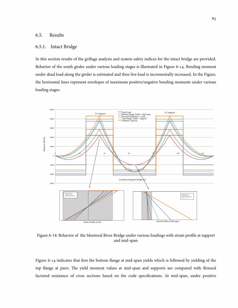
6.5. Results
6.5.1. Intact Bridge
In this section results of the grillage analysis and system safety indices for the intact bridge are provided.
Behavior of the south girder under various loading stages is illustrated in Figure -. Bending moment
under dead load along the girder is estimated and then live load is incrementally increased. In the Figure,
the horizontal lines represent envelopes of maximum positive/negative bending moments under various
loading stages.
Figure 6-14: Behavior of the Montreal River Bridge under various loadings with strain pro'le at supportand mid-span
Figure - indicates that 'rst the bottom 1ange at mid-span yields which is followed by yielding of the
top 1ange at piers. e yield moment values at mid-span and supports are compared with 1exural
factored resistance of cross sections based on the code speci'cations. At mid-span, under positive
!"####$
!%####$
!&####$
!'####$
!(####$
#$
(####$
'####$
&####$
#$ '#$ %#$ )#$ *#$ (##$ ('#$
Mom
ent (
kN.m
)
Loctation along the bridge (m)
Dead Load Bottom Flange Yields - Mid-span Factored Resistance - Code "Top Flange Yields - Support" Ultimate Capacity
CL Support CL Support
Strain Pro!le at Mid-span Strain Pro!le at Pier
Shaded area represents !<!y
Shaded area represents !<!y

bending, the concrete deck takes compression while code allows bottom 1ange of the steel girder to yield
in tension. erefore, the factored moment resistance of the cross section at mid-span is larger than the
bending moment for the initial yielding of the cross section. Meanwhile, the top 1ange of the cross
section at supports experiences tension under negative bending. e factored resistance moment at
supports is calculated for the Class III section by setting the stress at the top 1ange equal to the value of
steel yield stress including material reduction factor. erefore, factored moment resistance at support is
slightly smaller than the yield moment value for the cross section. e system reaches ultimate capacity
when the bottom 1ange at supports yields in compression and the class III section loses its rotational
capacity. As a result, although at this stage the cross section at mid-span has not reached its ultimate
capacity, the girder cannot take any further load. If the cross section at supports had enough rotational
capacity, live load could be increased to form a second plastic-hinge at mid-span and create a collapse
mechanism.
e above procedure is performed for live load cases described in Section . and results are tabulated
into groups. ree groups for two side-by-side trucks with three possible correlation factors and two
groups for the one truck loading event, given in Table -. Each of the 'rst three groups have load cases
for transverse truck placements and the last two groups have load cases each.
Group Two trucks side-by-side, correlation factor = .
Group Two trucks side-by-side, correlation factor = .
Group Two trucks side-by-side, correlation factor = .
Group One truck, right lane
Group One truck, le lane
Table 6-6: Description of 5 live load groups used to calculate results
e Load-De1ection response of the Montreal River Bridge for selected live load cases is presented in
Figure -. In the case of two-truck loading events, trucks are placed with their right axle . meters into
the traffic lanes. Similarly, single trucks are also placed at a curb distance of . meters. In Figure -, the
vertical axis on the right side shows the “Nominal Design Live Load Factor.” is is a measure of the
corresponding design load based on the CHBDC code and presents the number of two CL- trucks
including dynamic load factor and multi-lane reduction factor. e “Nominal Design Live Load Factor”
of . corresponds to the design live load of the bridge in terms of two CL- trucks. Figure - shows
that design load is very close to the load that causes the bottom 1ange to yield at mid-span. Results
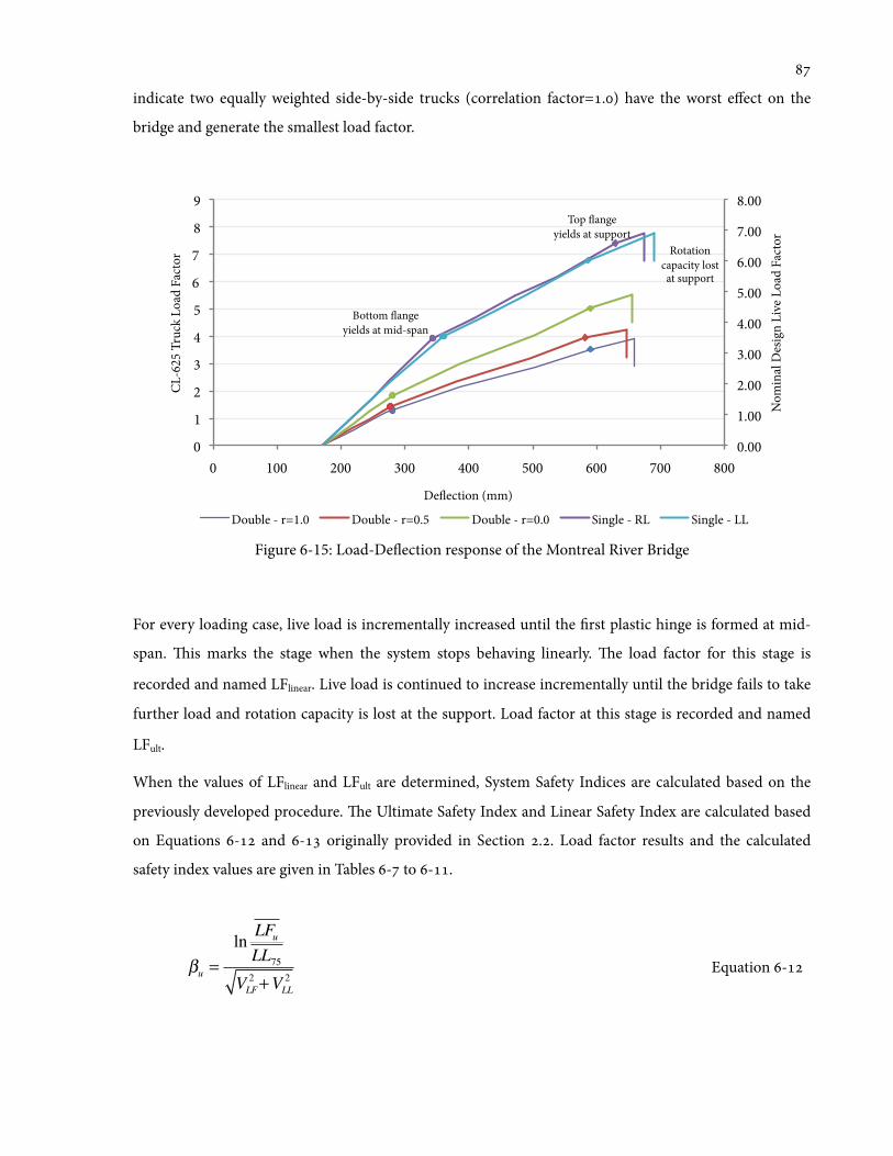
indicate two equally weighted side-by-side trucks (correlation factor=.) have the worst effect on the
bridge and generate the smallest load factor.
Figure 6-15: Load-De1ection response of the Montreal River Bridge
For every loading case, live load is incrementally increased until the 'rst plastic hinge is formed at mid-
span. is marks the stage when the system stops behaving linearly. e load factor for this stage is
recorded and named LFlinear. Live load is continued to increase incrementally until the bridge fails to take
further load and rotation capacity is lost at the support. Load factor at this stage is recorded and named
LFult.
When the values of LFlinear and LFult are determined, System Safety Indices are calculated based on the
previously developed procedure. e Ultimate Safety Index and Linear Safety Index are calculated based
on Equations - and - originally provided in Section .. Load factor results and the calculated
safety index values are given in Tables - to -.
βu =ln LFuLL75
VLF2 +VLL
2Equation -
Rotation capacity lost at support
Bottom !ange yields at mid-span
Top !ange yields at support
0.00
1.00
2.00
3.00
4.00
5.00
6.00
7.00
8.00
0
1
2
3
4
5
6
7
8
9
0 100 200 300 400 500 600 700 800
Nom
inal
Des
ign
Live
Loa
d Fa
ctor
CL-6
25 T
ruck
Loa
d Fa
ctor
De!ection (mm)
Double - r=1.0 Double - r=0.5 Double - r=0.0 Single - RL Single - LL
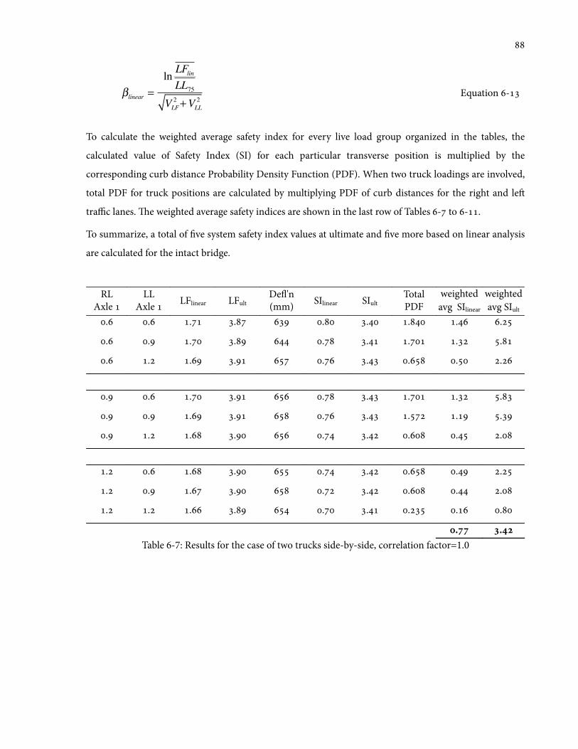
βlinear =ln LFlinLL75
VLF2 +VLL
2Equation -
To calculate the weighted average safety index for every live load group organized in the tables, the
calculated value of Safety Index (SI) for each particular transverse position is multiplied by the
corresponding curb distance Probability Density Function (PDF). When two truck loadings are involved,
total PDF for truck positions are calculated by multiplying PDF of curb distances for the right and le
traffic lanes. e weighted average safety indices are shown in the last row of Tables - to -.
To summarize, a total of 've system safety index values at ultimate and 've more based on linear analysis
are calculated for the intact bridge.
RLAxle
LLAxle LFlinear LFult
De1'n(mm) SIlinear SIult
TotalPDF
weightedavg SIlinear
weightedavg SIult
. . . . . . . . .
. . . . . . . . .
. . . . . . . . .
. . . . . . . . .
. . . . . . . . .
. . . . . . . . .
. . . . . . . . .
. . . . . . . . .
. . . . . . . . .
. .Table 6-7: Results for the case of two trucks side-by-side, correlation factor=1.0
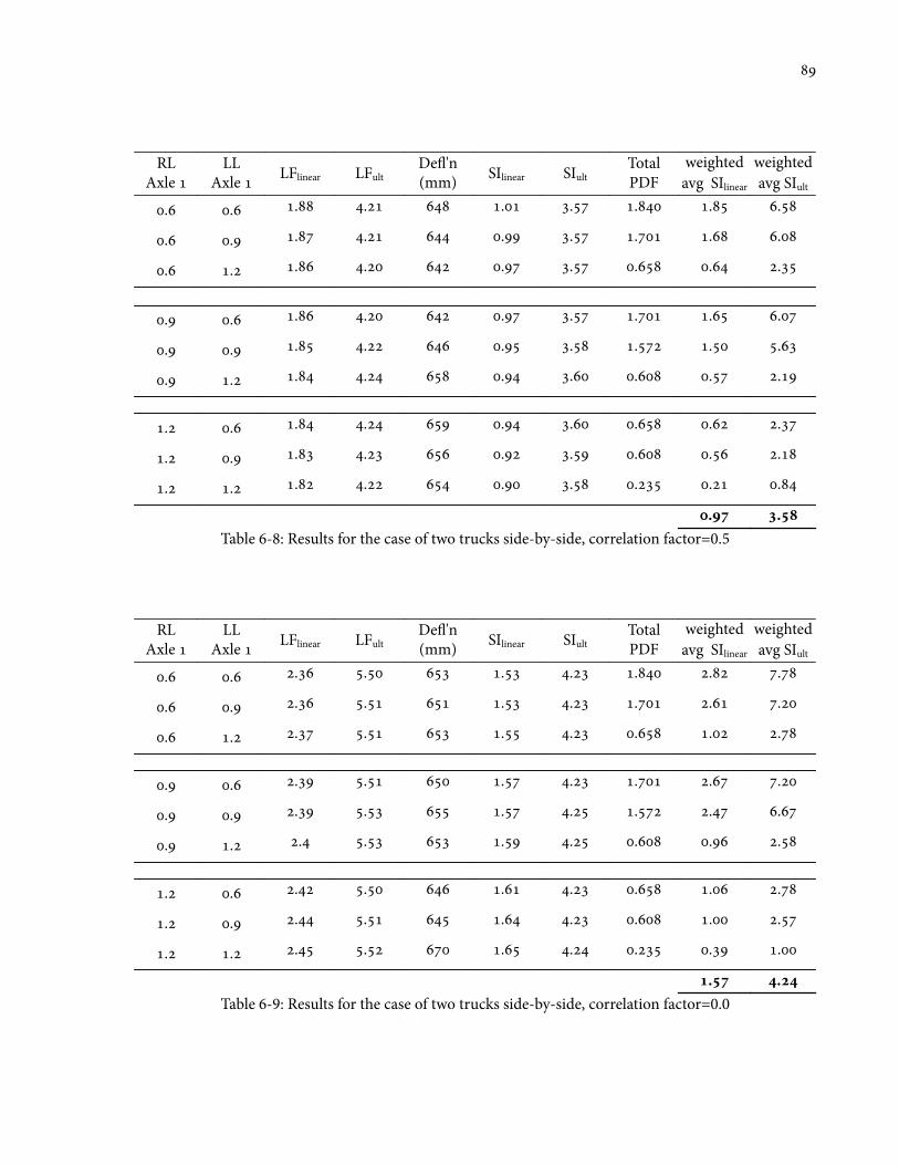
RLAxle
LLAxle LFlinear LFult
De1'n(mm) SIlinear SIult
TotalPDF
weightedavg SIlinear
weightedavg SIult
. . . . . . . . .
. . . . . . . . .
. . . . . . . . .
. . . . . . . . .
. . . . . . . . .
. . . . . . . . .
. . . . . . . . .
. . . . . . . . .
. . . . . . . . .
. .Table 6-8: Results for the case of two trucks side-by-side, correlation factor=0.5
RLAxle
LLAxle LFlinear LFult
De1'n(mm) SIlinear SIult
TotalPDF
weightedavg SIlinear
weightedavg SIult
. . . . . . . . .
. . . . . . . . .
. . . . . . . . .
. . . . . . . . .
. . . . . . . . .
. . . . . . . . .
. . . . . . . . .
. . . . . . . . .
. . . . . . . . .
. .Table 6-9: Results for the case of two trucks side-by-side, correlation factor=0.0
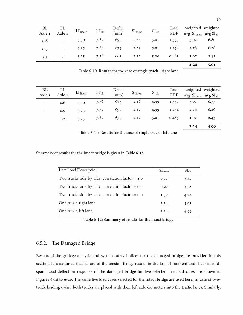
RLAxle
LLAxle LFlinear LFult
De1'n(mm) SIlinear SIult
TotalPDF
weightedavg SIlinear
weightedavg SIult
. - . . . . . . .
. - . . . . . . .
. - . . . . . . .
. .Table 6-10: Results for the case of single truck - right lane
RLAxle
LLAxle LFlinear LFult
De1'n(mm) SIlinear SIult
TotalPDF
weightedavg SIlinear
weightedavg SIult
- . . . . . . . .
- . . . . . . . .
- . . . . . . . .
. .Table 6-11: Results for the case of single truck - le lane
Summary of results for the intact bridge is given in Table -.
Live Load Description SIlinear SIult
Two trucks side-by-side, correlation factor = . . .
Two trucks side-by-side, correlation factor = . . .
Two trucks side-by-side, correlation factor = . . .
One truck, right lane . .
One truck, le lane . .
Table 6-12: Summary of results for the intact bridge
6.5.2. e Damaged Bridge
Results of the grillage analysis and system safety indices for the damaged bridge are provided in this
section. It is assumed that failure of the tension 1ange results in the loss of moment and shear at mid-
span. Load-de1ection response of the damaged bridge for 've selected live load cases are shown in
Figures - to -. e same live load cases selected for the intact bridge are used here. In case of two-
truck loading event, both trucks are placed with their le axle . meters into the traffic lanes. Similarly,
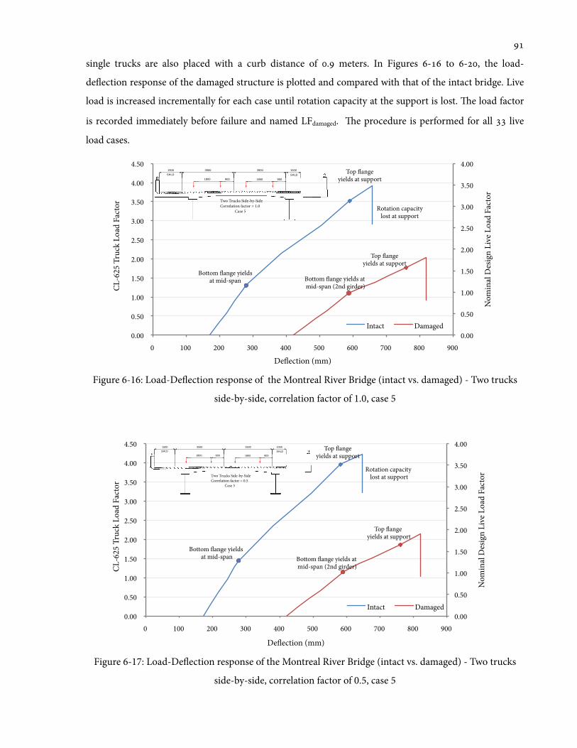
single trucks are also placed with a curb distance of . meters. In Figures - to -, the load-
de1ection response of the damaged structure is plotted and compared with that of the intact bridge. Live
load is increased incrementally for each case until rotation capacity at the support is lost. e load factor
is recorded immediately before failure and named LFdamaged. e procedure is performed for all live
load cases.
Figure 6-16: Load-De1ection response of the Montreal River Bridge (intact vs. damaged) - Two trucks
side-by-side, correlation factor of 1.0, case 5
Figure 6-17: Load-De1ection response of the Montreal River Bridge (intact vs. damaged) - Two trucks
side-by-side, correlation factor of 0.5, case 5
Bottom !ange yields at mid-span
Top !ange yields at support
Rotation capacity lost at support
Bottom !ange yields at mid-span (2nd girder)
Top !ange yields at support
0.00
0.50
1.00
1.50
2.00
2.50
3.00
3.50
4.00
0.00
0.50
1.00
1.50
2.00
2.50
3.00
3.50
4.00
4.50
0 100 200 300 400 500 600 700 800 900
Nom
inal
Des
ign
Live
Loa
d Fa
ctor
CL-6
25 T
ruck
Loa
d Fa
ctor
De!ection (mm)
Intact Damaged
1500 3500 3500 1000
900
SHLD SHLD
18009001800
Two Trucks Side-by-SideCorrelation factor = 1.0
Case 5
Bottom !ange yields at mid-span
Top !ange yields at support
Rotation capacity lost at support
Bottom !ange yields at mid-span (2nd girder)
Top !ange yields at support
0.00
0.50
1.00
1.50
2.00
2.50
3.00
3.50
4.00
0.00
0.50
1.00
1.50
2.00
2.50
3.00
3.50
4.00
4.50
0 100 200 300 400 500 600 700 800 900
Nom
inal
Des
ign
Live
Loa
d Fa
ctor
CL-6
25 T
ruck
Loa
d Fa
ctor
De!ection (mm)
Intact Damaged
1500 3500 3500 1000
900
SHLD SHLD
18009001800
Two Trucks Side-by-SideCorrelation factor = 0.5
Case 5
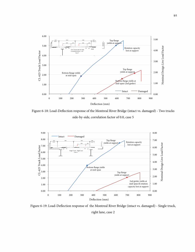
Figure 6-18: Load-De1ection response of the Montreal River Bridge (intact vs. damaged) - Two trucks
side-by-side, correlation factor of 0.0, case 5
Figure 6-19: Load-De1ection response of the Montreal River Bridge (intact vs. damaged) - Single truck,
right lane, case 2
Bottom !ange yields at mid-span
Top !ange yields at support
Rotation capacity lost at support
Bottom !ange yields at mid-span (2nd girder)
Top !ange yields at support
0.00
1.00
2.00
3.00
4.00
5.00
0.00
1.00
2.00
3.00
4.00
5.00
6.00
0 100 200 300 400 500 600 700 800 900
Nom
inal
Des
ign
Live
Loa
d Fa
ctor
CL-6
25 T
ruck
Loa
d Fa
ctor
De!ection (mm)
Intact Damaged
1500 3500 3500 1000
900
SHLD SHLD
18009001800
Two Trucks Side-by-SideCorrelation factor = 0.0
Case 5
Bottom !ange yields at mid-span
Top !ange yields at support Rotation capacity
lost at support
Top !ange yields at support
2nd girder yields at mid-span & rotation
capacity lost at support
0.00
1.00
2.00
3.00
4.00
5.00
6.00
7.00
8.00
0.00
1.00
2.00
3.00
4.00
5.00
6.00
7.00
8.00
9.00
0 100 200 300 400 500 600 700 800 900
Nom
inal
Des
ign
Live
Loa
d Fa
ctor
CL-6
25 T
ruck
Loa
d Fa
ctor
De!ection (mm)
Intact Damaged 1500 3500 3500 1000
SHLD SHLD
9001800
Single Truck - Right LaneCase 2
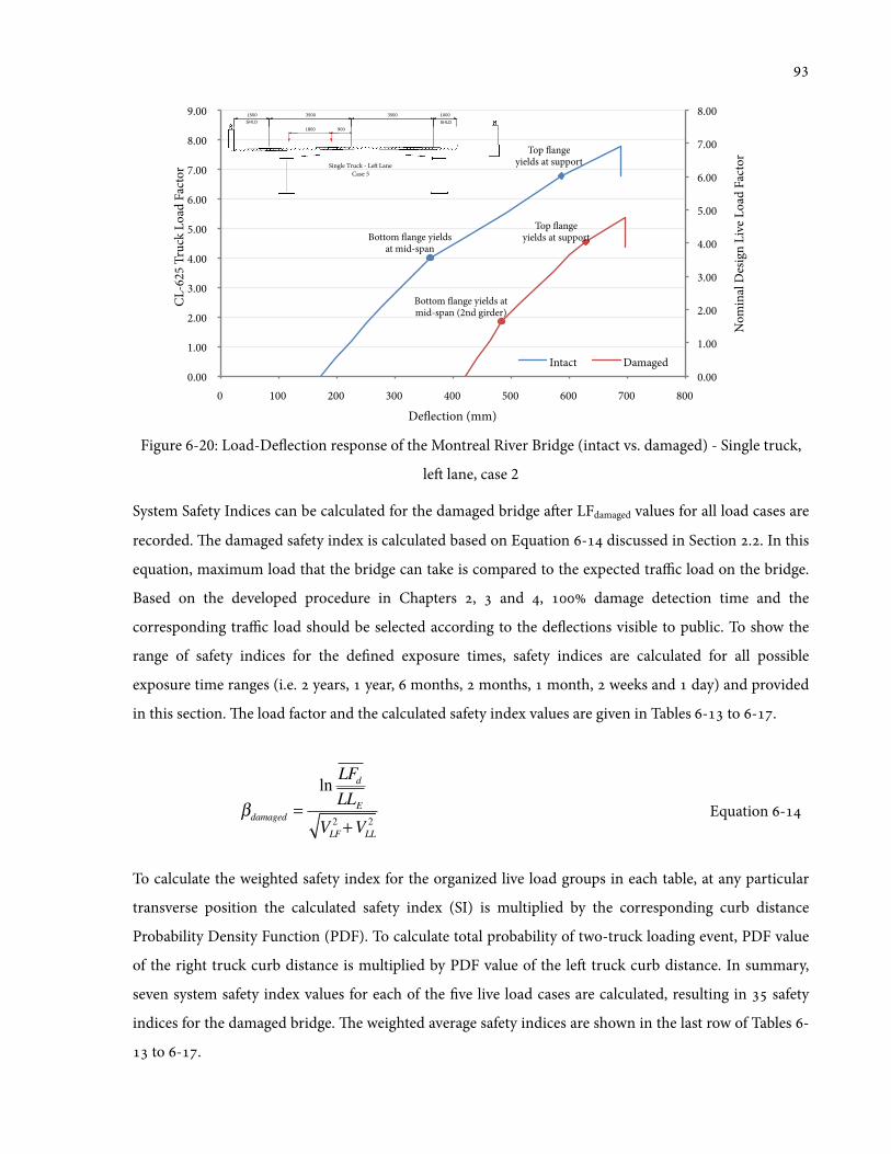
Figure 6-20: Load-De1ection response of the Montreal River Bridge (intact vs. damaged) - Single truck,
le lane, case 2
System Safety Indices can be calculated for the damaged bridge aer LFdamaged values for all load cases are
recorded. e damaged safety index is calculated based on Equation - discussed in Section .. In this
equation, maximum load that the bridge can take is compared to the expected traffic load on the bridge.
Based on the developed procedure in Chapters , and , damage detection time and the
corresponding traffic load should be selected according to the de1ections visible to public. To show the
range of safety indices for the de'ned exposure times, safety indices are calculated for all possible
exposure time ranges (i.e. years, year, months, months, month, weeks and day) and provided
in this section. e load factor and the calculated safety index values are given in Tables - to -.
!damaged =
lnLFd
LLE
VLF2+VLL
2
! Equation -
To calculate the weighted safety index for the organized live load groups in each table, at any particular
transverse position the calculated safety index (SI) is multiplied by the corresponding curb distance
Probability Density Function (PDF). To calculate total probability of two-truck loading event, PDF value
of the right truck curb distance is multiplied by PDF value of the le truck curb distance. In summary,
seven system safety index values for each of the 've live load cases are calculated, resulting in safety
indices for the damaged bridge. e weighted average safety indices are shown in the last row of Tables -
to -.
Bottom !ange yields at mid-span
Top !ange yields at support
Bottom !ange yields at mid-span (2nd girder)
Top !ange yields at support
0.00
1.00
2.00
3.00
4.00
5.00
6.00
7.00
8.00
0.00
1.00
2.00
3.00
4.00
5.00
6.00
7.00
8.00
9.00
0 100 200 300 400 500 600 700 800
Nom
inal
Des
ign
Live
Loa
d Fa
ctor
CL-6
25 T
ruck
Loa
d Fa
ctor
De!ection (mm)
Intact Damaged
1500 3500 3500 1000
900
SHLD SHLD
1800
Single Truck - Le! Lane Case 5
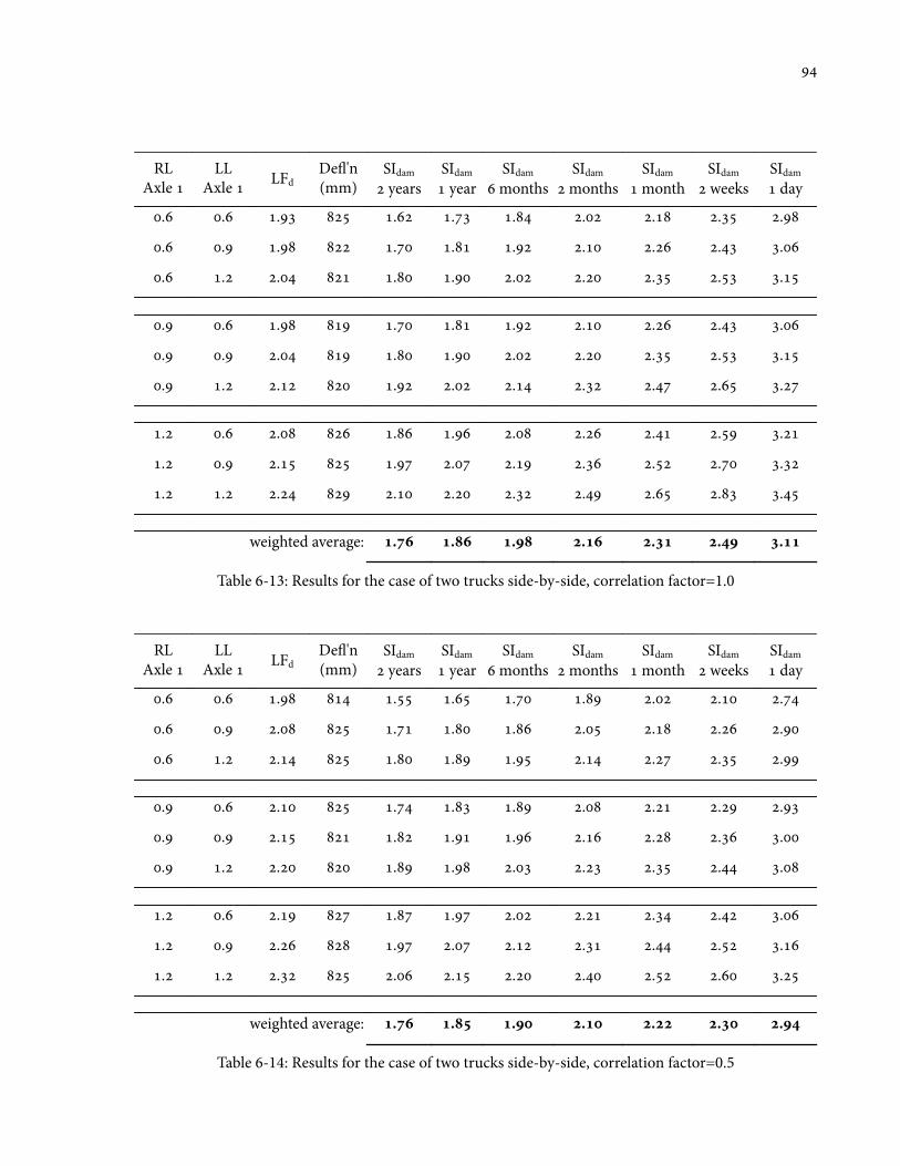
RLAxle
LLAxle LFd
De1'n(mm)
SIdam
yearsSIdam
yearSIdam
monthsSIdam
monthsSIdam
monthSIdam
weeksSIdam
day
. . . . . . . . . .
. . . . . . . . . .
. . . . . . . . . .
. . . . . . . . . .
. . . . . . . . . .
. . . . . . . . . .
. . . . . . . . . .
. . . . . . . . . .
. . . . . . . . . .
weighted average: . . . . . . .
Table 6-13: Results for the case of two trucks side-by-side, correlation factor=1.0
RLAxle
LLAxle LFd
De1'n(mm)
SIdam
yearsSIdam
yearSIdam
monthsSIdam
monthsSIdam
monthSIdam
weeksSIdam
day
. . . . . . . . . .
. . . . . . . . . .
. . . . . . . . . .
. . . . . . . . . .
. . . . . . . . . .
. . . . . . . . . .
. . . . . . . . . .
. . . . . . . . . .
. . . . . . . . . .
weighted average: . . . . . . .
Table 6-14: Results for the case of two trucks side-by-side, correlation factor=0.5
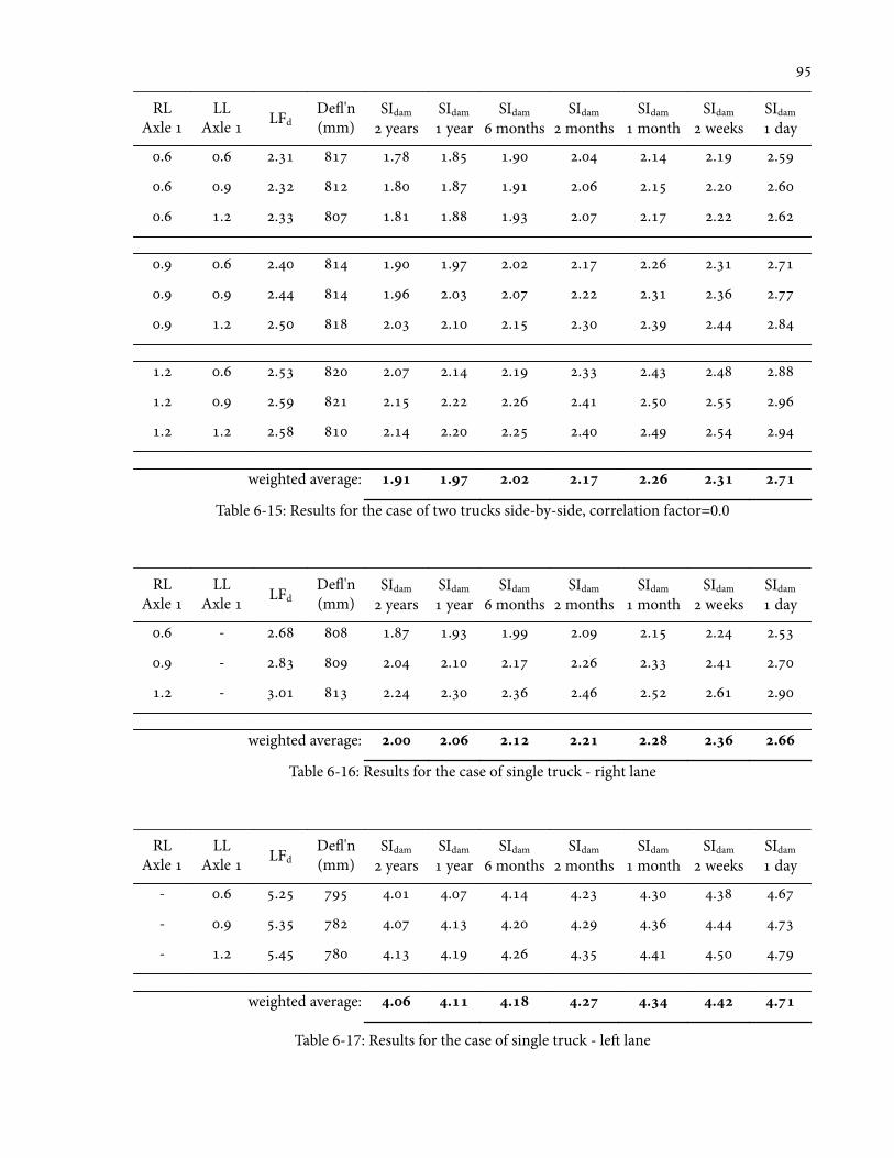
RLAxle
LLAxle LFd
De1'n(mm)
SIdam
yearsSIdam
yearSIdam
monthsSIdam
monthsSIdam
monthSIdam
weeksSIdam
day
. . . . . . . . . .
. . . . . . . . . .
. . . . . . . . . .
. . . . . . . . . .
. . . . . . . . . .
. . . . . . . . . .
. . . . . . . . . .
. . . . . . . . . .
. . . . . . . . . .
weighted average: . . . . . . .
Table 6-15: Results for the case of two trucks side-by-side, correlation factor=0.0
RLAxle
LLAxle LFd
De1'n(mm)
SIdam
yearsSIdam
yearSIdam
monthsSIdam
monthsSIdam
monthSIdam
weeksSIdam
day
. - . . . . . . . .
. - . . . . . . . .
. - . . . . . . . .
weighted average: . . . . . . .
Table 6-16: Results for the case of single truck - right lane
RLAxle
LLAxle LFd
De1'n(mm)
SIdam
yearsSIdam
yearSIdam
monthsSIdam
monthsSIdam
monthSIdam
weeksSIdam
day
- . . . . . . . . .
- . . . . . . . . .
- . . . . . . . . .
weighted average: . . . . . . .
Table 6-17: Results for the case of single truck - le lane
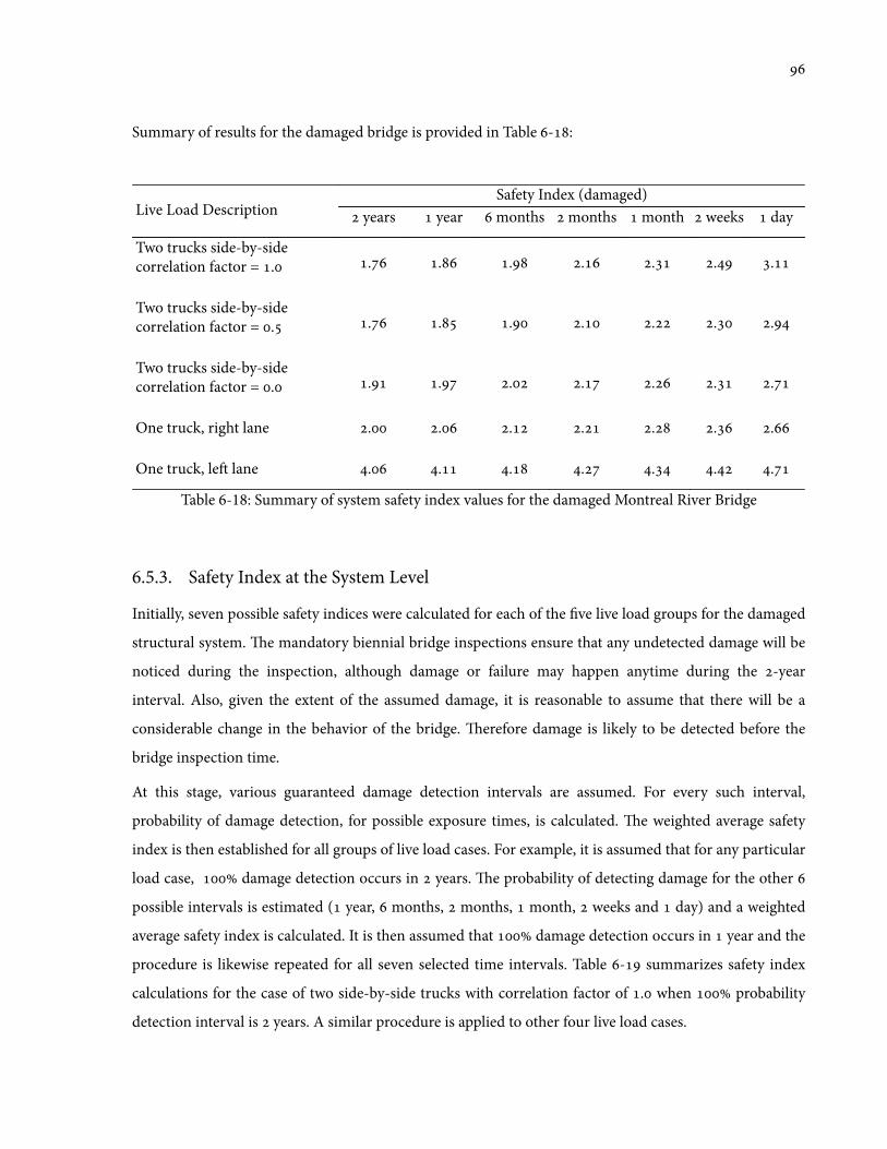
Summary of results for the damaged bridge is provided in Table -:
Live Load DescriptionSafety Index (damaged)
years year months months month weeks day
Two trucks side-by-side correlation factor = . . . . . . . .
Two trucks side-by-sidecorrelation factor = . . . . . . . .
Two trucks side-by-sidecorrelation factor = . . . . . . . .
One truck, right lane . . . . . . .
One truck, le lane . . . . . . .
Table 6-18: Summary of system safety index values for the damaged Montreal River Bridge
6.5.3. Safety Index at the System Level
Initially, seven possible safety indices were calculated for each of the 've live load groups for the damaged
structural system. e mandatory biennial bridge inspections ensure that any undetected damage will be
noticed during the inspection, although damage or failure may happen anytime during the -year
interval. Also, given the extent of the assumed damage, it is reasonable to assume that there will be a
considerable change in the behavior of the bridge. erefore damage is likely to be detected before the
bridge inspection time.
At this stage, various guaranteed damage detection intervals are assumed. For every such interval,
probability of damage detection, for possible exposure times, is calculated. e weighted average safety
index is then established for all groups of live load cases. For example, it is assumed that for any particular
load case, damage detection occurs in years. e probability of detecting damage for the other
possible intervals is estimated ( year, months, months, month, weeks and day) and a weighted
average safety index is calculated. It is then assumed that damage detection occurs in year and the
procedure is likewise repeated for all seven selected time intervals. Table - summarizes safety index
calculations for the case of two side-by-side trucks with correlation factor of . when probability
detection interval is years. A similar procedure is applied to other four live load cases.
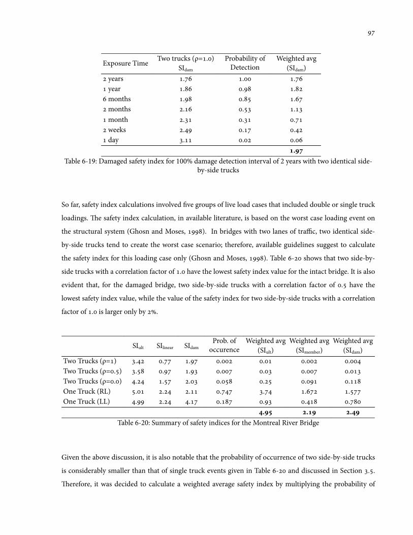
Exposure Time Two trucks (ρ=.)SIdam
Probability ofDetection
Weighted avg(SIdam)
years . . . year . . . months . . . months . . . month . . . weeks . . . day . . .
.Table 6-19: Damaged safety index for 100% damage detection interval of 2 years with two identical side-
by-side trucks
So far, safety index calculations involved 've groups of live load cases that included double or single truck
loadings. e safety index calculation, in available literature, is based on the worst case loading event on
the structural system (Ghosn and Moses, ). In bridges with two lanes of traffic, two identical side-
by-side trucks tend to create the worst case scenario; therefore, available guidelines suggest to calculate
the safety index for this loading case only (Ghosn and Moses, ). Table - shows that two side-by-
side trucks with a correlation factor of . have the lowest safety index value for the intact bridge. It is also
evident that, for the damaged bridge, two side-by-side trucks with a correlation factor of . have the
lowest safety index value, while the value of the safety index for two side-by-side trucks with a correlation
factor of . is larger only by .
SIult SIlinear SIdamProb. of
occurenceWeighted avg
(SIult)Weighted avg
(SImember)Weighted avg
(SIdam)Two Trucks (ρ=) . . . . . . .Two Trucks (ρ=.) . . . . . . .Two Trucks (ρ=.) . . . . . . .One Truck (RL) . . . . . . .One Truck (LL) . . . . . . .
. . .Table 6-20: Summary of safety indices for the Montreal River Bridge
Given the above discussion, it is also notable that the probability of occurrence of two side-by-side trucks
is considerably smaller than that of single truck events given in Table - and discussed in Section ..
erefore, it was decided to calculate a weighted average safety index by multiplying the probability of
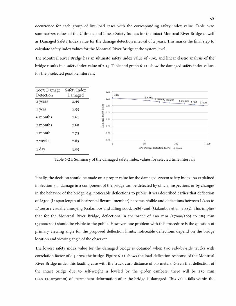
occurrence for each group of live load cases with the corresponding safety index value. Table -
summarizes values of the Ultimate and Linear Safety Indices for the intact Montreal River Bridge as well
as Damaged Safety Index value for the damage detection interval of years. is marks the 'nal step to
calculate safety index values for the Montreal River Bridge at the system level.
e Montreal River Bridge has an ultimate safety index value of ., and linear elastic analysis of the
bridge results in a safety index value of .. Table and graph - show the damaged safety index values
for the selected possible intervals.
Damage Detection
Safety IndexDamaged
2 years 1 year 6 months 2 months 1 month 2 weeks 1 day
0.00
0.50
1.00
1.50
2.00
2.50
3.00
3.50
1 10 100 1000
Dam
aged
Safe
ty In
dex
100% Damage Detection (days) - Log scale
years .
year .
months .
months .
month .
weeks .
day .
Table 6-21: Summary of the damaged safety index values for selected time intervals
Finally, the decision should be made on a proper value for the damaged system safety index. As explained
in Section ., damage in a component of the bridge can be detected by official inspections or by changes
in the behavior of the bridge, e.g. noticeable de1ections to public. It was described earlier that de1ection
of L/ (L: span length of horizontal 1exural member) becomes visible and de1ections between L/ to
L/ are visually annoying (Galambos and Ellingwood, ) and (Galambos et al., ). is implies
that for the Montreal River Bridge, de1ections in the order of mm (/) to mm
(/) should be visible to the public. However, one problem with this procedure is the question of
primary viewing angle for the proposed de1ection limits; noticeable de1ections depend on the bridge
location and viewing angle of the observer.
e lowest safety index value for the damaged bridge is obtained when two side-by-side trucks with
correlation factor of . cross the bridge. Figure - shows the load-de1ection response of the Montreal
River Bridge under this loading case with the truck curb distance of . meters. Given that de1ection of
the intact bridge due to self-weight is leveled by the girder cambers, there will be mm
(-=mm) of permanent deformation aer the bridge is damaged. is value falls within the
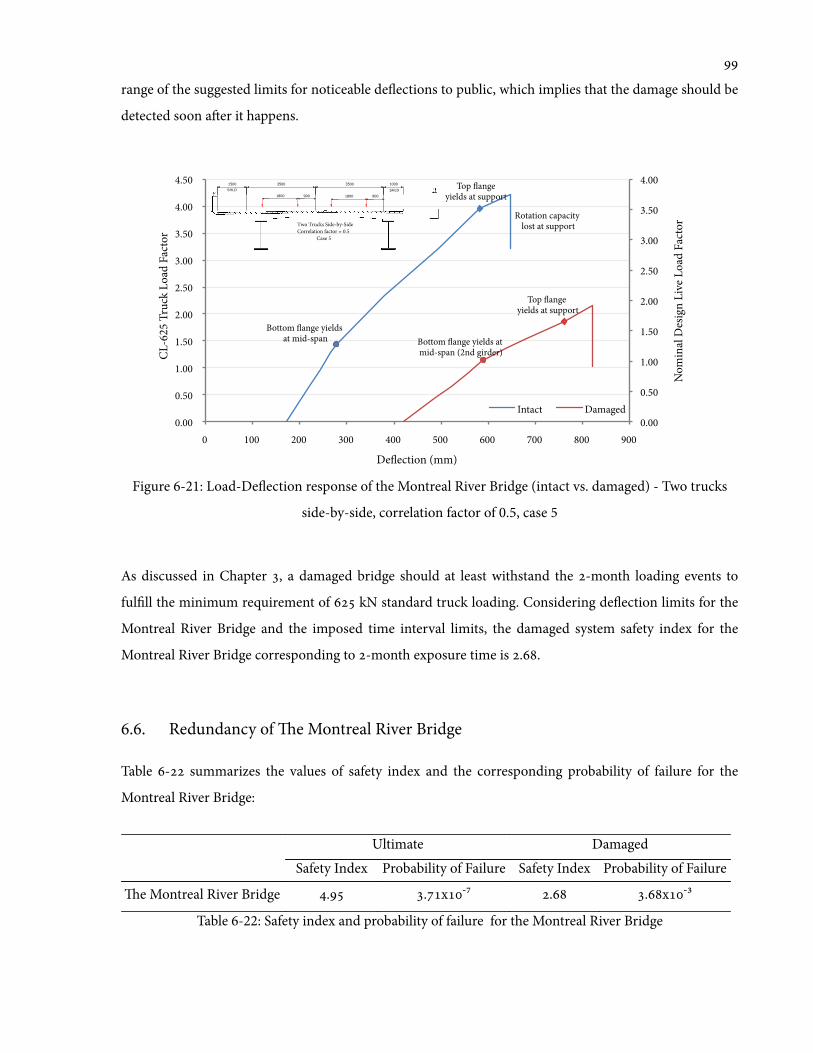
range of the suggested limits for noticeable de1ections to public, which implies that the damage should be
detected soon aer it happens.
Figure 6-21: Load-De1ection response of the Montreal River Bridge (intact vs. damaged) - Two trucks
side-by-side, correlation factor of 0.5, case 5
As discussed in Chapter , a damaged bridge should at least withstand the -month loading events to
ful'll the minimum requirement of kN standard truck loading. Considering de1ection limits for the
Montreal River Bridge and the imposed time interval limits, the damaged system safety index for the
Montreal River Bridge corresponding to -month exposure time is ..
6.6. Redundancy of e Montreal River Bridge
Table - summarizes the values of safety index and the corresponding probability of failure for the
Montreal River Bridge:
Ultimate Damaged
Safety Index Probability of Failure Safety Index Probability of Failure
e Montreal River Bridge . .x⁷ . .x3
Table 6-22: Safety index and probability of failure for the Montreal River Bridge
Bottom !ange yields at mid-span
Top !ange yields at support
Rotation capacity lost at support
Bottom !ange yields at mid-span (2nd girder)
Top !ange yields at support
0.00
0.50
1.00
1.50
2.00
2.50
3.00
3.50
4.00
0.00
0.50
1.00
1.50
2.00
2.50
3.00
3.50
4.00
4.50
0 100 200 300 400 500 600 700 800 900
Nom
inal
Des
ign
Live
Loa
d Fa
ctor
CL-6
25 T
ruck
Loa
d Fa
ctor
De!ection (mm)
Intact Damaged
1500 3500 3500 1000
900
SHLD SHLD
18009001800
Two Trucks Side-by-SideCorrelation factor = 0.5
Case 5

e Montreal River Bridge consists of twin steel girders with a composite deck slab. e ultimate safety
index of the system is calculated to be .. When the cross section at mid-span of one steel girder is
damaged, the system safety index is reduced t .. e probability of failure for the intact bridge in a
-year life span is smaller than ⁶ while the bridge in damaged condition has a failure probability
considerably smaller than .x1. e Montreal River Bridge satis'es all the requirements imposed in
the proposed guidelines established in this thesis.
Twin steel girder bridges are generally considered to be non-redundant systems. is may be true for
single span simply supported structures. e three-span Montreal River Bridge has one degree of
indeterminacy in the longitudinal direction; therefore, aer capacity of one girder at mid-span is lost,
applied load is redistributed and built-in reserve capacity of the central piers allow the damaged system to
withstand reasonable load.
In order to further analyze the situation, when βe is the element reliability index and βs is the system
reliability index, then values of βe and βs are only equal for a single-path component. A multi-path system
consists of at least two parallel elements. For such a system, when βe equals to . and the two members
are completely uncorrelated, the system reliability index βs equals to .. In bridges, members are
generally partially correlated. erefore, the system safety index of a bridge with two parallel components
has a value between . and ., depending on the degree of the correlation between members. (Nowak
and Szerszen, ) It can be concluded that safety index value of . for the Montreal River Bridge is
reasonable, given that the bridge components are designed with a safety index of ..
Finally, based on the developed guidelines, the Montreal River Bridge at intact condition is considered to
be safe and when one girder is damaged at mid-span, it redistributes the load and takes reasonable traffic.
It can be concluded that twin girder bridges can be designed with enough redundancy to ensure safety.
Chapter 7
Bridge Structures with Concrete Double-T Girder and ExternalUnbonded Post-tensioning
In this chapter, the previously developed guidelines are used to evaluate redundancy of a new structural
system with two webs. is is an attempt to validate new concrete bridge structural systems that have high
intrinsic robustness while minimizing material consumption and economic premium. Bridges with short
to medium span lengths (i.e. m to m) represent major part of the bridge industry; therefore, they
are of great economical importance to the society. In most of Canada, the CPCI (Canadian Precast
Prestressed Concrete Institute) slab-on-girder system is the preferred structural system for spans up to
meters. e CPCI slab-on-girder system consists of multiple parallel precast, pre-tensioned concrete
girders with cast-in-place concrete deck slab. Although design and construction of such systems are
reasonably straightforward, they make a relatively inefficient use of material. Recent studies at the
University of Toronto have resulted in the development of design concepts, with Concrete Double-T
Girder and External Unbonded Post-tensioning, that make efficient use of high compressive strength of
high-performance and ultra high-performance concrete (Li, ). e following topics will be addressed
in this chapter:
() Brief description of the bridge concept;
() Structural model of the bridge to perform nonlinear analysis of the structure and obtain
ultimate capacity of the bridge at intact and damaged conditions;
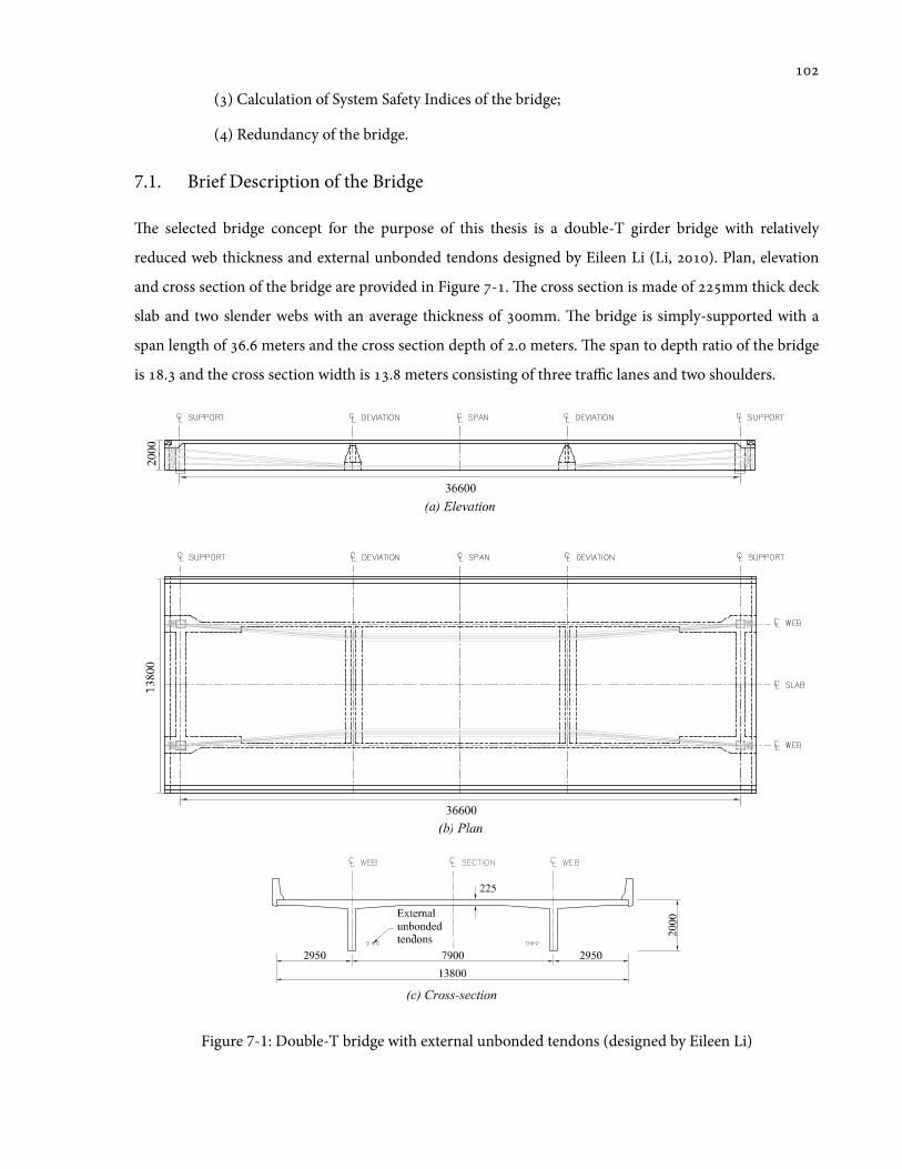
() Calculation of System Safety Indices of the bridge;
() Redundancy of the bridge.
7.1. Brief Description of the Bridge
e selected bridge concept for the purpose of this thesis is a double-T girder bridge with relatively
reduced web thickness and external unbonded tendons designed by Eileen Li (Li, ). Plan, elevation
and cross section of the bridge are provided in Figure -. e cross section is made of mm thick deck
slab and two slender webs with an average thickness of mm. e bridge is simply-supported with a
span length of . meters and the cross section depth of . meters. e span to depth ratio of the bridge
is . and the cross section width is . meters consisting of three traffic lanes and two shoulders.
Figure 7-1: Double-T bridge with external unbonded tendons (designed by Eileen Li)
!

e bridge structure is post-tensioned in transverse and longitudinal directions. In the transverse
direction, the deck slab is post-tensioned with internal 1at-duct tendons and in the longitudinal
direction, the system is post-tensioned with external unbonded tendons. Two deviation diaphragms are
provided along the span length to accommodate deviation of external unbonded tendons (Li, ).
Detailed drawings of the bridge are provided in Appendix D.
In the transverse direction, there are three tendons spaced at mm intervals in the deck slab of every
precast segment where each tendon consists of strands. In the longitudinal direction, prestressing
consists of strands per web, grouped into tendons, where the tendons are arranged in a harped
pro'le with a horizontal segment between the two deviations, shown in Figure -a.
e bridge is designed with a concrete compressive strength of MPa and mm diameter prestressing
steel with MPa speci'ed tensile strength. e material properties of the bridge are summarized in
Table -.
Material Strength Modulus of Elasticity
Concrete (Deck) Speci'ed compressive strength:f 'c = 70MPa
Cracking strength:
fcr = 0.4 f 'c = 3.35MPa
Ec = ( f 'c + 6900)(γ c
2300)1.5
Ec = 36300MPa
Reinforcing Steel (Grade ) Yield strength:fy = 400MPa
Es = 200000 MPa
Prestressing Steel Diameter: mm Astrand= mm2
Speci'ed tensile strength:fpu = 1860MPa
Yield strength:fpy = 0.9 fpu = 1674MPa
Ep = 200000MPa
Table 7-1: Material Properties for the double-T bridge with externally unbonded tendons
e bridge is designed according to the Canadian Highway Bridge Design Code (CHBDC) (CSA, a).
e stress-strain relationship of material assumed in the analysis of the bridge is shown in Figure -. e
stress-strain response of the ductile reinforcing steel is de'ned as bilinear where the relation is linear up
to the yield stress fy followed by a yield plateau. e stress-strain relation of the prestressing steel is also
de'ned as bilinear and the yield stress value fpy is assumed as . (times) of the ultimate tensile strength.

Figure 7-2: Material stress-strain relationship for the double-T bridge with unbonded tendons
e behavior of concrete is de'ned with Popovics high strength concrete model. Equation - is applied
to represent the pre and post peak concrete compression responses:
fcf 'c
=n(εcf / ε 'c )
n −1+ (εcf / ε 'c )nk Equation -
where n = 0.8 + f 'c17(MPa) Equation -
k = 0.67 + f 'c62
≥ 1.0 Equation -
e effective tendon force under service loads is always less than the jacking force due to prestress losses.
e losses include friction loss, anchor set loss, losses due to concrete creep, shrinkage and relaxation of
prestressing steel aer transfer. In design of the bridge concept, the effective prestressing force in tendons,
aer all losses are considered, is calculated to be .fpu (Li, ). erefore, use of - mm strands
per web results in an effective prestressing force of kN.
7.2. Structural Behavior - Intact Bridge
7.2.1. Longitudinal Flexure
e reliability assessment of bridges requires an extensive study of the bridge behavior under various
loading conditions just before failure. In members with bonded tendons, the strain in tendon is directly
related to the strain in concrete at tendon level; therefore, the plane section theory is applicable to both
!sy
f y
E s1
f s
!s !py
fpy
Ep1
fp
!p
!0.9fpu
Reinforcing Steel Prestressing SteelConcrete
fc
c!
f 'c
!'c
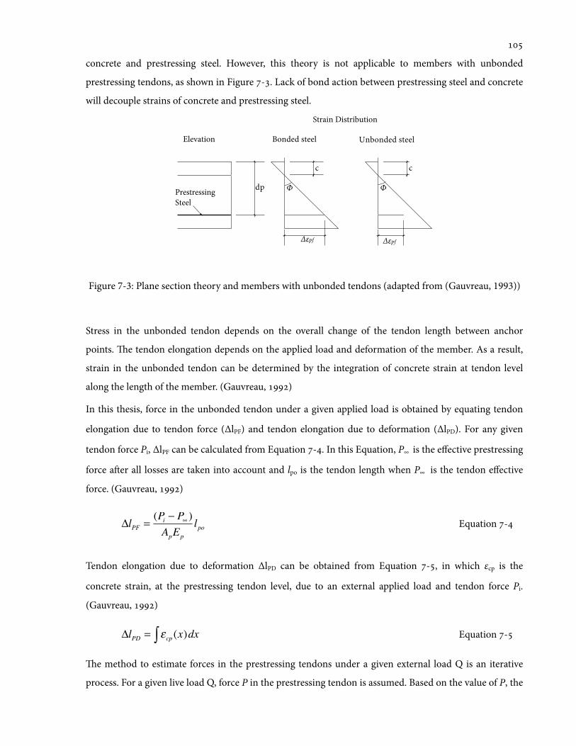
concrete and prestressing steel. However, this theory is not applicable to members with unbonded
prestressing tendons, as shown in Figure -. Lack of bond action between prestressing steel and concrete
will decouple strains of concrete and prestressing steel.
Figure 7-3: Plane section theory and members with unbonded tendons (adapted from (Gauvreau, 1993))
Stress in the unbonded tendon depends on the overall change of the tendon length between anchor
points. e tendon elongation depends on the applied load and deformation of the member. As a result,
strain in the unbonded tendon can be determined by the integration of concrete strain at tendon level
along the length of the member. (Gauvreau, )
In this thesis, force in the unbonded tendon under a given applied load is obtained by equating tendon
elongation due to tendon force (ΔlPF) and tendon elongation due to deformation (ΔlPD). For any given
tendon force Pi, ΔlPF can be calculated from Equation -. In this Equation, P∞ is the effective prestressing
force aer all losses are taken into account and lpo is the tendon length when P∞ is the tendon effective
force. (Gauvreau, )
ΔlPF =(Pi − P∞ )ApEp
lpo Equation -
Tendon elongation due to deformation ΔlPD can be obtained from Equation -, in which εcp is the
concrete strain, at the prestressing tendon level, due to an external applied load and tendon force Pi.
(Gauvreau, )
ΔlPD = εcp (x)dx∫ Equation -
e method to estimate forces in the prestressing tendons under a given external load Q is an iterative
process. For a given live load Q, force P in the prestressing tendon is assumed. Based on the value of P, the
dp
c
!"pf
#
Elevation Bonded steel
Prestressing Steel
c
!"pf
#
Unbonded steel
Strain Distribution

elongation due to tendon force (ΔlPF) is calculated; demand and capacity at various locations are also
determined. Given the values of demand and capacity, tendon elongation due to deformation (ΔlPD) is
calculated and compared to ΔlPF. If the two elongation values do not match, force P in the prestressing
tendon is adjusted accordingly. e iterative process is continued until elongation values from Equations
- and - match.
Since there are many live load cases to be considered in the reliability analysis of the bridge, an Excel
Spreadsheet with a built-in Visual Basic Macro is prepared to improve accuracy and speed of the analysis.
7.2.2. Second-order Effects in External Tendons
When loads are applied to a prestressed structure, internal tendons de1ect together with the concrete
member, but external tendons are free to displace between attachment points (i.e. anchorages and
deviators) and tend not to follow member displacements. e result is a continuous change in the
eccentricity of external prestressing tendons under various loading conditions. is is referred to as
second order effects. Figure - shows the change in the pro'le of the internal and external tendons.
Figure 7-4: Internal and external unbonded tendons
Internal Unbonded Tendons
dp=dpo
dp<dpo
External Unbonded Tendons (with two deviators)
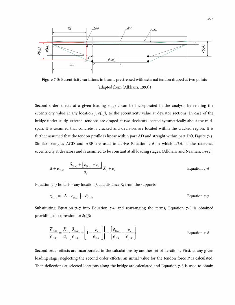
Figure 7-5: Eccentricity variations in beams prestressed with external tendon draped at two points
(adapted from (Alkhairi, 1993))
Second order effects at a given loading stage i can be incorporated in the analysis by relating the
eccentricity value at any location j, ē(i,j), to the eccentricity value at deviator sections. In case of the
bridge under study, external tendons are draped at two deviators located symmetrically about the mid-
span. It is assumed that concrete is cracked and deviators are located within the cracked region. It is
further assumed that the tendon pro'le is linear within part AD and straight within part DO, Figure -.
Similar triangles ACD and ABE are used to derive Equation - in which e(i,d) is the reference
eccentricity at deviators and is assumed to be constant at all loading stages. (Alkhairi and Naaman, )
Δ + e(i, j ) =δ(i,d ) + e(i,d ) − es⎡⎣ ⎤⎦
aoX j + es Equation -
Equation - holds for any location j, at a distance Xj from the supports:
e(i, j ) = Δ + e(i, j )⎡⎣ ⎤⎦ − δ(i, j ) Equation -
Substituting Equation - into Equation - and rearranging the terms, Equation - is obtained
providing an expression for ē(i,j):
e(i, j )e(i,d )
=Xj
ao
δ(i,d )e(i,d )
+ 1− ese(i,d )
⎡
⎣⎢⎢
⎤
⎦⎥⎥
⎧⎨⎪
⎩⎪
⎫⎬⎪
⎭⎪−
δ(i, j )e(i,d )
−ese(i,d )
⎧⎨⎪
⎩⎪
⎫⎬⎪
⎭⎪Equation -
Second order effects are incorporated in the calculations by another set of iterations. First, at any given
loading stage, neglecting the second order effects, an initial value for the tendon force P is calculated.
en de1ections at selected locations along the bridge are calculated and Equation - is used to obtain
!(i,d)
!(i,l)!(i,j)
"(i,j
)
e(i,j
)
e(i,d
)
e s
Xj
ao
A B C
DE}#
O
C.G.
revised eccentricity values. e new values are used to update total bending moment and the tendon
elongation due to deformation (ΔlPD). Iteration is repeated if ΔlPD is not equal to ΔlPF.
7.2.3. Shear Resistance - the CAN/CSA S6.06 Provisions
Shear resistance of the double-T girder bridge with external unbonded tendons is calculated according to
the CAN/CSA S. CHBDC shear provisions (CSA, a). e bridge concept was originally designed
according to these speci'cations (Li, ).
e total shear resistance in a cross section Vr results from the contribution of shear resistance by tensile
stresses in concrete Vc, transverse steel reinforcement Vs and shear resistance by the component of
prestressing force in tendons acting in the direction of applied shear Vp, shown in Equation -:
Vr = Vc +Vs +Vp Equation -
e value of Vc contributed from the tensile stress in concrete is obtained from:
Vc = φcβ f 'cbwdv Equation -
where β is a factor that accounts for the cracked concrete, √f 'c accounts for the concrete tensile strength
and is limited to MPa, bw is the effective beam width, dv is the effective shear depth and Φc is the
material reduction factor taken as ..
Equation - shows factored shear resistance of the transverse reinforcement:
Vs =φsAv fydv cotθ
sEquation -
where Av is the area of the shear reinforcement within distance s between stirrups, fy is the speci'ed yield
strength of the reinforcing steel, θ is the angle of inclination of diagonal compressive stresses with
longitudinal axis of the member and Φs is the resistance factor for the reinforcing steel that is taken as ..
Computation of β and θ using the General Method is shown in Equations - and -:
β =0.40
(1+1500ε x )×
1300(1000 + sze )
Equation -
θ = 29 + 7000ε x Equation -

β is related to the average concrete tensile strain and crack spacing. e crack spacing parameter sze
depends on the crack control characteristics of the longitudinal reinforcement and is a function of the
member depth, longitudinal reinforcement spacing and aggregate size. Both β and θ are functions of
concrete longitudinal strain εx , shown in Equation -:
ε x =M f / dv +Vf −Vp + 0.5N f − Ap fpe
2(EsAs + EpAp )Equation -
According to code provisions, εx is calculated at mid-depth of the member and is dependent on the
1exural moment, shear, axial and prestressing forces. Mf , Vf and Nf are applied sectional forces taken as
positive values. Vp is the component of prestressing force in the direction of applied shear. Ap represents
the area of prestressing and fpe is the effective prestressing force in tendons aer all losses are considered.
e CHBDC provisions limit the value of εx to a range of -.×3 to .×3.
7.3. Structural Behavior - Damaged Bridge
Behavior of the bridge concept under damaged condition, with the speci'c structural system (double-T
girder with external unbonded tendons), is different than the multi-girder bridge studied in the previous
chapter. In reliability analysis of the Montreal River Bridge, it was assumed that the bottom 1ange of the
steel girder was hit by a truck, damaged and 1exural capacity of one girder was lost at mid-span. Similar
to the Montreal River Bridge, here too, it is assumed that a truck hits the bridge from below and part of
the web is damaged at mid-span while the tendons remain intact.
e effect due to sudden loss of one web at mid-span on the double-T concept with external unbonded
post-tensioning is different than that of the Montreal River Bridge. At mid-span, the external tendons
take tension, and the top portion of the concrete deck takes compression. erefore, the 1exural capacity
of the damaged cross section remains the same and does not change under positive bending. It should be
noted that the stiffness of one web at mid-span becomes less than the other and live load distribution
between the two webs may slightly be different. Nevertheless, behavior of the bridge under live load with
the sudden loss of one web is not considered to be a critical damaging case.
e double-T system with external unbonded post-tensioning is designed to maximize efficient use of
concrete and prestressing tendons. Slender webs with an average thickness of mm are selected for the
cross section resulting in a light structure. Absence of live load on the bridge creates negative bending at
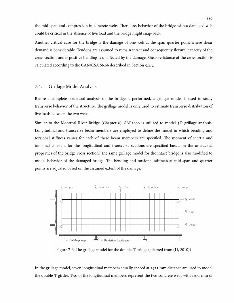
the mid-span and compression in concrete webs. erefore, behavior of the bridge with a damaged web
could be critical in the absence of live load and the bridge might snap-back.
Another critical case for the bridge is the damage of one web at the span quarter point where shear
demand is considerable. Tendons are assumed to remain intact and consequently 1exural capacity of the
cross section under positive bending is unaffected by the damage. Shear resistance of the cross section is
calculated according to the CAN/CSA S. described in Section ...
7.4. Grillage Model Analysis
Before a complete structural analysis of the bridge is performed, a grillage model is used to study
transverse behavior of the structure. e grillage model is only used to estimate transverse distribution of
live loads between the two webs.
Similar to the Montreal River Bridge (Chapter ), SAP is utilized to model D grillage analysis.
Longitudinal and transverse beam members are employed to de'ne the model in which bending and
torsional stiffness values for each of these beam members are speci'ed. e moment of inertia and
torsional constant for the longitudinal and transverse sections are speci'ed based on the uncracked
properties of the bridge cross section. e same grillage model for the intact bridge is also modi'ed to
model behavior of the damaged bridge. e bending and torsional stiffness at mid-span and quarter
points are adjusted based on the assumed extent of the damage.
Figure 7-6: e grillage model for the double-T bridge (adapted from (Li, 2010))
In the grillage model, seven longitudinal members equally spaced at mm distance are used to model
the double-T girder. Two of the longitudinal members represent the two concrete webs with mm of
!
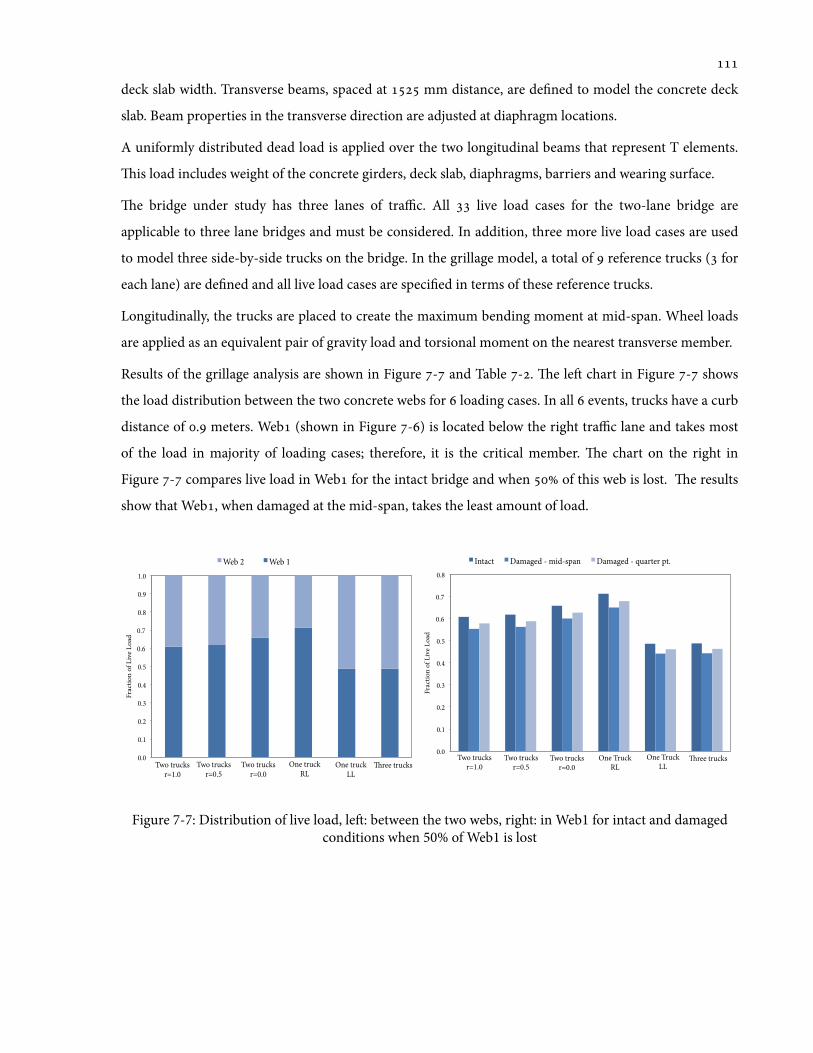
deck slab width. Transverse beams, spaced at mm distance, are de'ned to model the concrete deck
slab. Beam properties in the transverse direction are adjusted at diaphragm locations.
A uniformly distributed dead load is applied over the two longitudinal beams that represent T elements.
is load includes weight of the concrete girders, deck slab, diaphragms, barriers and wearing surface.
e bridge under study has three lanes of traffic. All live load cases for the two-lane bridge are
applicable to three lane bridges and must be considered. In addition, three more live load cases are used
to model three side-by-side trucks on the bridge. In the grillage model, a total of reference trucks ( for
each lane) are de'ned and all live load cases are speci'ed in terms of these reference trucks.
Longitudinally, the trucks are placed to create the maximum bending moment at mid-span. Wheel loads
are applied as an equivalent pair of gravity load and torsional moment on the nearest transverse member.
Results of the grillage analysis are shown in Figure - and Table -. e le chart in Figure - shows
the load distribution between the two concrete webs for loading cases. In all events, trucks have a curb
distance of . meters. Web (shown in Figure -) is located below the right traffic lane and takes most
of the load in majority of loading cases; therefore, it is the critical member. e chart on the right in
Figure - compares live load in Web for the intact bridge and when of this web is lost. e results
show that Web, when damaged at the mid-span, takes the least amount of load.
Figure 7-7: Distribution of live load, le: between the two webs, right: in Web1 for intact and damagedconditions when 50% of Web1 is lost
Two trucks r=1.0
Two trucks r=0.5
Two trucks r=0.0
One truck RL
One truck LL
!ree trucks 0.0
0.1
0.2
0.3
0.4
0.5
0.6
0.7
0.8
0.9
1.0
Frac
tion
of L
ive L
oad
Web 2 Web 1
Two trucks r=1.0
Two trucks r=0.5
Two trucks r=0.0
One Truck RL
One Truck LL
!ree trucks 0.0
0.1
0.2
0.3
0.4
0.5
0.6
0.7
0.8
Frac
tion
of L
ive L
oad
Intact Damaged - mid-span Damaged - quarter pt.
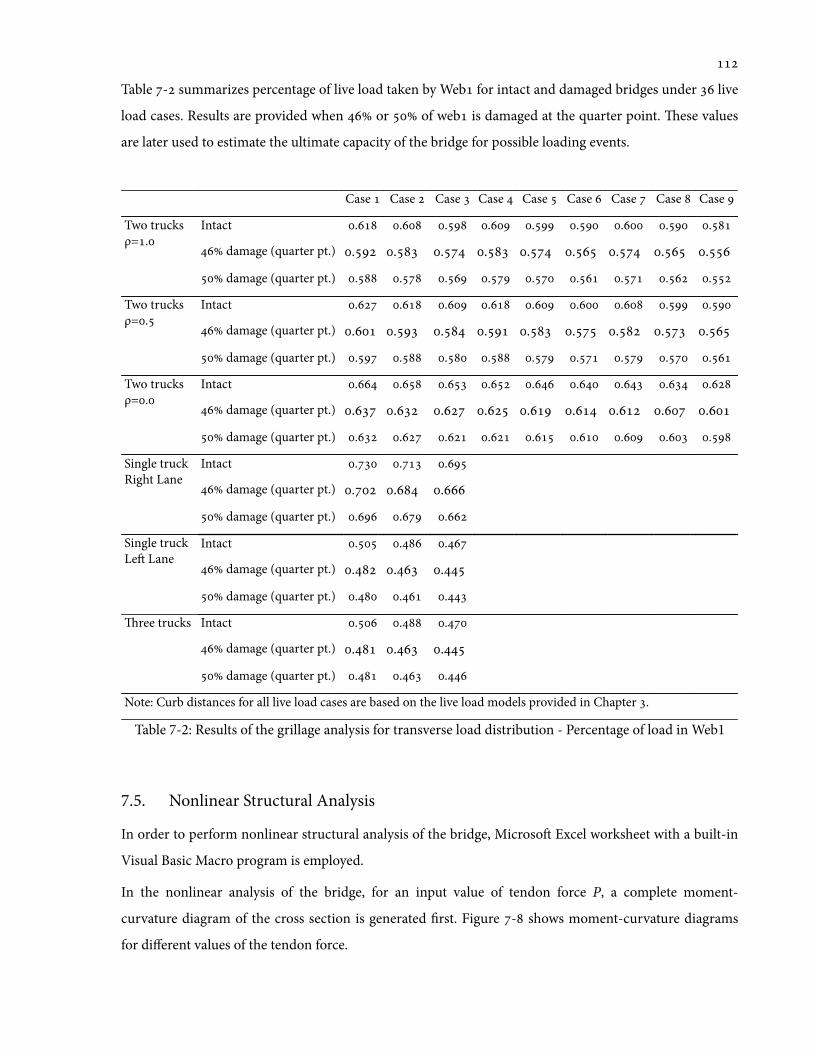
Table - summarizes percentage of live load taken by Web for intact and damaged bridges under live
load cases. Results are provided when or of web is damaged at the quarter point. ese values
are later used to estimate the ultimate capacity of the bridge for possible loading events.
Case Case Case Case Case Case Case Case Case
Two trucksρ=.
Intact . . . . . . . . .
damage (quarter pt.) . . . . . . . . .
damage (quarter pt.) . . . . . . . . .
Two trucks ρ=.
Intact . . . . . . . . .
damage (quarter pt.) . . . . . . . . .
damage (quarter pt.) . . . . . . . . .
Two trucks ρ=.
Intact . . . . . . . . .
damage (quarter pt.) . . . . . . . . .
damage (quarter pt.) . . . . . . . . .
Single truckRight Lane
Intact . . .
damage (quarter pt.) . . .
damage (quarter pt.) . . .
Single truckLe Lane
Intact . . .
damage (quarter pt.) . . .
damage (quarter pt.) . . .
ree trucks Intact . . .
damage (quarter pt.) . . .
damage (quarter pt.) . . .
Note: Curb distances for all live load cases are based on the live load models provided in Chapter .
Table 7-2: Results of the grillage analysis for transverse load distribution - Percentage of load in Web1
7.5. Nonlinear Structural Analysis
In order to perform nonlinear structural analysis of the bridge, Microso Excel worksheet with a built-in
Visual Basic Macro program is employed.
In the nonlinear analysis of the bridge, for an input value of tendon force P, a complete moment-
curvature diagram of the cross section is generated 'rst. Figure - shows moment-curvature diagrams
for different values of the tendon force.
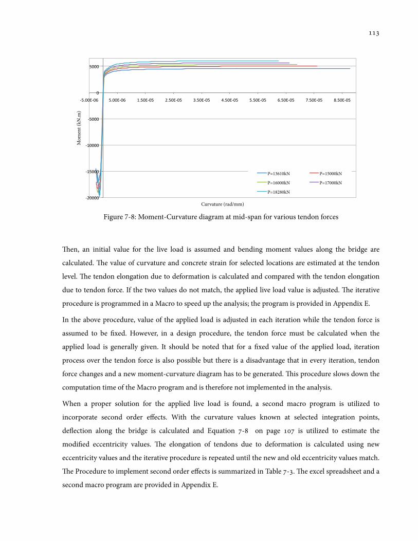
Figure 7-8: Moment-Curvature diagram at mid-span for various tendon forces
en, an initial value for the live load is assumed and bending moment values along the bridge are
calculated. e value of curvature and concrete strain for selected locations are estimated at the tendon
level. e tendon elongation due to deformation is calculated and compared with the tendon elongation
due to tendon force. If the two values do not match, the applied live load value is adjusted. e iterative
procedure is programmed in a Macro to speed up the analysis; the program is provided in Appendix E.
In the above procedure, value of the applied load is adjusted in each iteration while the tendon force is
assumed to be 'xed. However, in a design procedure, the tendon force must be calculated when the
applied load is generally given. It should be noted that for a 'xed value of the applied load, iteration
process over the tendon force is also possible but there is a disadvantage that in every iteration, tendon
force changes and a new moment-curvature diagram has to be generated. is procedure slows down the
computation time of the Macro program and is therefore not implemented in the analysis.
When a proper solution for the applied live load is found, a second macro program is utilized to
incorporate second order effects. With the curvature values known at selected integration points,
de1ection along the bridge is calculated and Equation - on page is utilized to estimate the
modi'ed eccentricity values. e elongation of tendons due to deformation is calculated using new
eccentricity values and the iterative procedure is repeated until the new and old eccentricity values match.
e Procedure to implement second order effects is summarized in Table -. e excel spreadsheet and a
second macro program are provided in Appendix E.
!"####$
!%&###$
!%####$
!&###$
#$
&###$
!&'##(!#)$ &'##(!#)$ %'&#(!#&$ "'&#(!#&$ *'&#(!#&$ +'&#(!#&$ &'&#(!#&$ )'&#(!#&$ ,'&#(!#&$ -'&#(!#&$
Mom
ent (
kN.m
)
Curvature (rad/mm)
P=13610kN P=15000kN
P=16000kN P=17000kN
P=18280kN

Step Assume tendon force P - guess an initial applied load.
Step Calculate tendon elongation due to force. ΔlPF =(Pi − P∞ )ApEp
lpo
Step Calculate total applied moment (due to dead load, live load and prestressing force).
Step Calculate curvature and concrete strain at tendon level along the bridge using moment-
curvature response for the assumed tendon force.
Step Calculate tendon elongation due to deformation. ΔlPD = εcp (x)dx∫Step Check the difference in tendon elongation from Steps and .
Step If tendon elongations calculated in Steps and do no match, change applied load value
and repeat from step .
Second order effects
Step Calculate de1ections along the bridge.
Step Update tendon eccentricity values along the bridge. e(i, j )
e(i,d )=Xj
ao
δ(i,d )e(i,d )
+ 1− ese(i,d )
⎡
⎣⎢⎢
⎤
⎦⎥⎥
⎧⎨⎪
⎩⎪
⎫⎬⎪
⎭⎪−
δ(i, j )e(i,d )
−ese(i,d )
⎧⎨⎪
⎩⎪
⎫⎬⎪
⎭⎪
Step Calculate total applied moment (due to dead load, live load and prestressing force).
Step Calculate curvature and concrete strain at tendon level along the bridge using moment-
curvature response for the assumed tendon force.
Step Calculate tendon elongation due to deformation. ΔlPD = εcp (x)dx∫Step Check the difference in tendon elongation from Steps and .
Step If tendon elongations calculated in Steps and do no match, repeat steps and ,
change applied load value and continue from step .
Table 7-3: Step by step procedure for structural analysis of bridges with external unbonded tendons
7.6. Results
7.6.1. Intact Bridge
e results of nonlinear analysis and safety indices for the intact bridge are provided in this section.
Initially, behavior of the intact bridge is studied without inclusion of second order effects. e graph on
the le in Figure - shows load-de1ection response of the intact bridge under two identical side-by-side
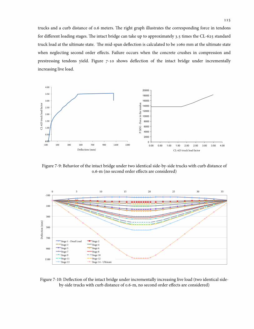
trucks and a curb distance of . meters. e right graph illustrates the corresponding force in tendons
for different loading stages. e intact bridge can take up to approximately . times the CL- standard
truck load at the ultimate state. e mid-span de1ection is calculated to be mm at the ultimate state
when neglecting second order effects. Failure occurs when the concrete crushes in compression and
prestressing tendons yield. Figure - shows de1ection of the intact bridge under incrementally
increasing live load.
Figure 7-9: Behavior of the intact bridge under two identical side-by-side trucks with curb distance of.-m (no second order effects are considered)
Figure 7-10: De1ection of the intact bridge under incrementally increasing live load (two identical side-by-side trucks with curb distance of .-m, no second order effects are considered)
!"!!#
!"$!#
%"!!#
%"$!#
&"!!#
&"$!#
'"!!#
'"$!#
("!!#
)%!!# %!!# '!!# $!!# *!!# +!!# %%!!# %'!!#
CL-6
25 tr
uck
load
fact
or
De!ection (mm)
0
2000
4000
6000
8000
10000
12000
14000
16000
18000
20000
0.00 0.50 1.00 1.50 2.00 2.50 3.00 3.50 4.00
P (k
N) -
For
ce in
the t
endo
n
CL-625 truck load factor
-100
100
300
500
700
900
1100
0 5 10 15 20 25 30 35
De!
ectio
n (m
m)
Stage 1 - Dead Load Stage 2 Stage 3 Stage 4 Stage 5 Stage 6 Stage 7 Stage 8 Stage 9 Stage 10 Stage 11 Stage 12 Stage 13 Stage 14 - Ultimate

Aer the initial behavior of the bridge is studied, second order effects of the externally unbonded tendons
are included in the nonlinear analysis of the intact bridge. Figure - shows the modi'ed de1ections of
the bridge under incrementally increasing live loads. When the prestressing force in tendons is kN
( of the yielding force value) de1ection at mid-span is estimated to be about mm. is implies
that the value of tendon eccentricity is dropped by as shown in Figure -.
Figure 7-11: De1ection of the intact bridge under incrementally increasing live load with second order
effects (two identical side-by-side trucks with curb distance of .-m)
Figure 7-12: Bending moment and change in eccentricity of the double-T system (prestressing
force=16500kN)
-100
0
100
200
300
400
500
600
0 5 10 15 20 25 30 35
De!
ectio
n (m
m)
Stage 1 - Dead Load Stage 2 Stage 3 Stage 4 Stage 5 Stage 6 Stage 7 Stage 8 - Ultimate
-2.5
-2
-1.5
-1
-0.5
0
Dep
th (m
)
Centroid - de!ected Tendon pro"le - de!ected
Centroid - original Tendon pro"le - original
Prestressing force =16500kN !"#$$$%
!"&$$$%
!"$$$$%
!'$$$%
!($$$%
!#$$$%
!&$$$%
$%
&$$$%
#$$$%
($$$%
'$$$%
$% &% #% (% '% "$% "&% "#% "(% "'%
Mto
tal (
Mp+
MQ
) kN
.m
Location along the bridge (m)
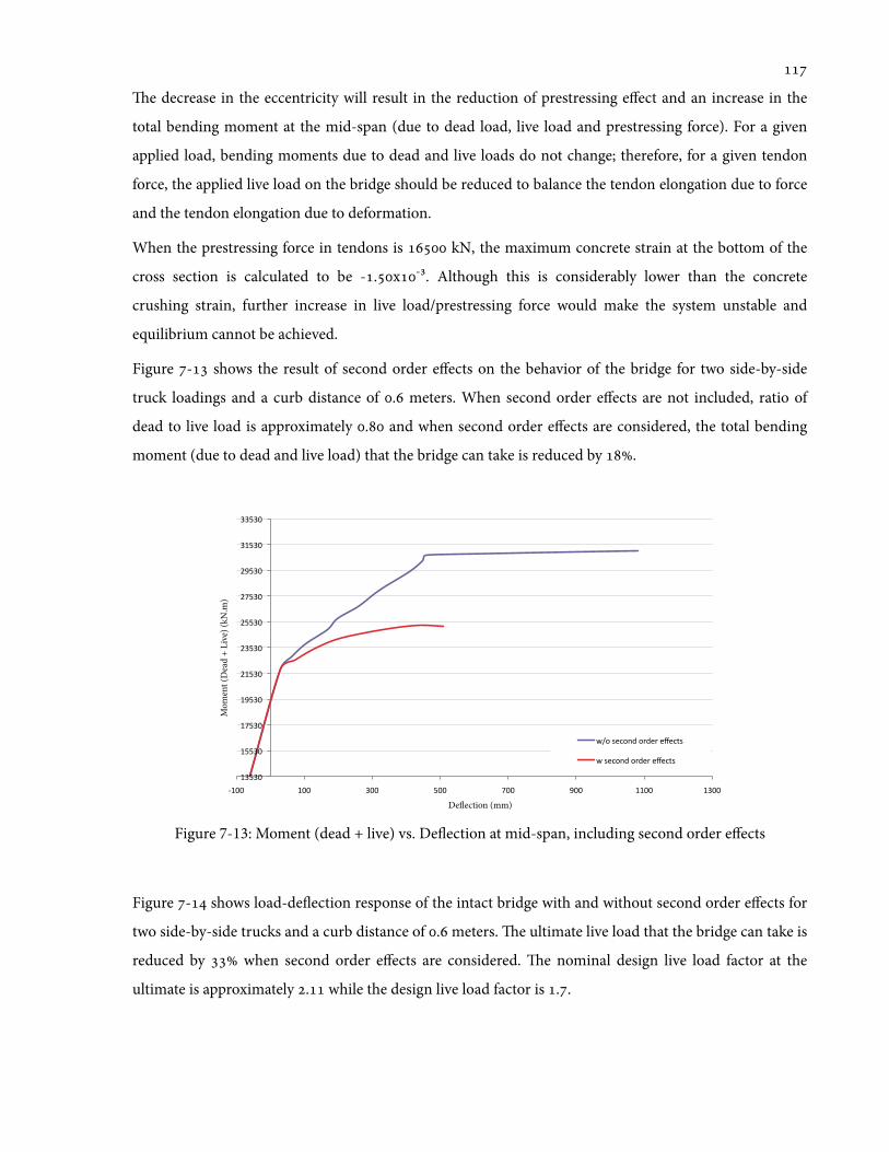
e decrease in the eccentricity will result in the reduction of prestressing effect and an increase in the
total bending moment at the mid-span (due to dead load, live load and prestressing force). For a given
applied load, bending moments due to dead and live loads do not change; therefore, for a given tendon
force, the applied live load on the bridge should be reduced to balance the tendon elongation due to force
and the tendon elongation due to deformation.
When the prestressing force in tendons is kN, the maximum concrete strain at the bottom of the
cross section is calculated to be -.x3. Although this is considerably lower than the concrete
crushing strain, further increase in live load/prestressing force would make the system unstable and
equilibrium cannot be achieved.
Figure - shows the result of second order effects on the behavior of the bridge for two side-by-side
truck loadings and a curb distance of . meters. When second order effects are not included, ratio of
dead to live load is approximately . and when second order effects are considered, the total bending
moment (due to dead and live load) that the bridge can take is reduced by .
Figure 7-13: Moment (dead + live) vs. De1ection at mid-span, including second order effects
Figure - shows load-de1ection response of the intact bridge with and without second order effects for
two side-by-side trucks and a curb distance of . meters. e ultimate live load that the bridge can take is
reduced by when second order effects are considered. e nominal design live load factor at the
ultimate is approximately . while the design live load factor is ..
!"#"$%
!##"$%
!&#"$%
!'#"$%
(!#"$%
("#"$%
(##"$%
(&#"$%
('#"$%
"!#"$%
""#"$%
)!$$% !$$% "$$% #$$% &$$% '$$% !!$$% !"$$%
Mom
ent (
Dea
d +
Live
) (kN
.m)
De!ection (mm)
*+,%-./,01%,21.2%.3./4-%
*%-./,01%,21.2%.3./4-%
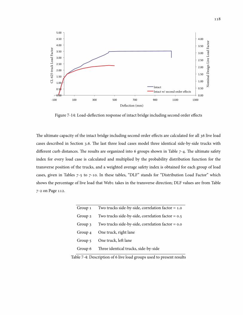
Figure 7-14: Load-de1ection response of intact bridge including second order effects
e ultimate capacity of the intact bridge including second order effects are calculated for all live load
cases described in Section .. e last three load cases model three identical side-by-side trucks with
different curb distances. e results are organized into groups shown in Table -. e ultimate safety
index for every load case is calculated and multiplied by the probability distribution function for the
transverse position of the trucks, and a weighted average safety index is obtained for each group of load
cases, given in Tables - to -. In these tables, “DLF” stands for “Distribution Load Factor” which
shows the percentage of live load that Web takes in the transverse direction; DLF values are from Table
- on Page .
Group Two trucks side-by-side, correlation factor = .
Group Two trucks side-by-side, correlation factor = .
Group Two trucks side-by-side, correlation factor = .
Group One truck, right lane
Group One truck, le lane
Group ree identical trucks, side-by-side
Table 7-4: Description of 6 live load groups used to present results
!"!!#
!"$!#
%"!!#
%"$!#
&"!!#
&"$!#
'"!!#
'"$!#
("!!#
!"!!#
!"$!#
%"!!#
%"$!#
&"!!#
&"$!#
'"!!#
'"$!#
("!!#
("$!#
$"!!#
)%!!# %!!# '!!# $!!# *!!# +!!# %%!!# %'!!#
Nom
inal
Des
ign
Live
Loa
d Fa
ctor
CL-6
25 tr
uck
Load
Fac
tor
De!ection (mm)
Intact Intact w/ second order e"ects
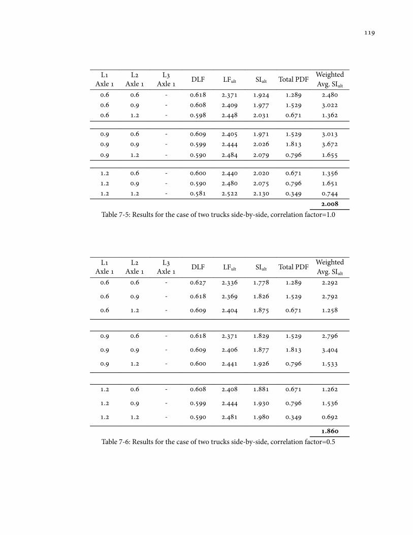
LAxle
LAxle
LAxle DLF LFult SIult Total PDF Weighted
Avg. SIult
. . - . . . . .. . - . . . . .. . - . . . . .
. . - . . . . .. . - . . . . .. . - . . . . .
. . - . . . . .. . - . . . . .. . - . . . . .
.Table 7-5: Results for the case of two trucks side-by-side, correlation factor=1.0
LAxle
LAxle
LAxle DLF LFult SIult Total PDF Weighted
Avg. SIult
. . - . . . . .
. . - . . . . .
. . - . . . . .
. . - . . . . .
. . - . . . . .
. . - . . . . .
. . - . . . . .
. . - . . . . .
. . - . . . . .
.Table 7-6: Results for the case of two trucks side-by-side, correlation factor=0.5
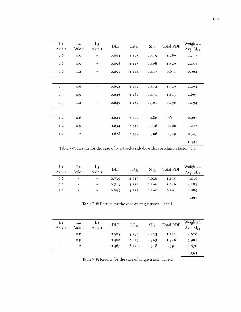
LAxle
LAxle
LAxle DLF LFult SIult Total PDF Weighted
Avg. SIult
. . - . . . . .
. . - . . . . .
. . - . . . . .
. . - . . . . .
. . - . . . . .
. . - . . . . .
. . - . . . . .
. . - . . . . .
. . - . . . . .
.Table 7-7: Results for the case of two trucks side-by-side, correlation factor=0.0
LAxle
LAxle
LAxle DLF LFult SIult Total PDF Weighted
Avg. SIult
. - - . . . . .. - - . . . . .. - - . . . . .
.Table 7-8: Results for the case of single truck - lane 1
LAxle
LAxle
LAxle DLF LFult SIult Total PDF Weighted
Avg. SIult
- . - . . . . .- . - . . . . .- . - . . . . .
.Table 7-9: Results for the case of single truck - lane 2
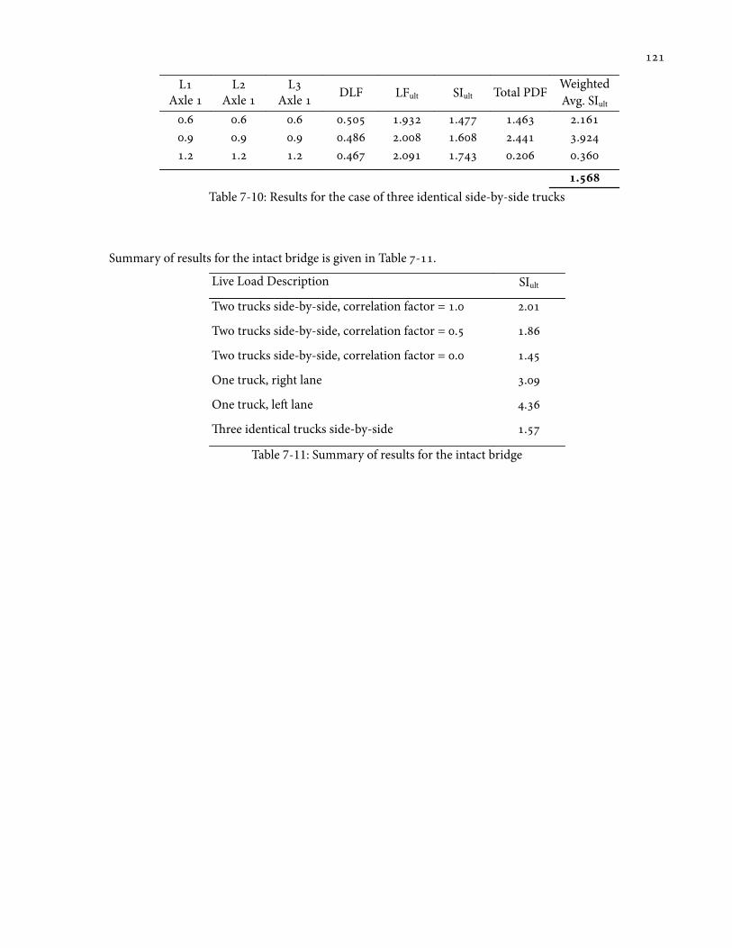
LAxle
LAxle
LAxle DLF LFult SIult Total PDF Weighted
Avg. SIult
. . . . . . . .. . . . . . . .. . . . . . . .
.Table 7-10: Results for the case of three identical side-by-side trucks
Summary of results for the intact bridge is given in Table -.
Live Load Description SIult
Two trucks side-by-side, correlation factor = . .
Two trucks side-by-side, correlation factor = . .
Two trucks side-by-side, correlation factor = . .
One truck, right lane .
One truck, le lane .
ree identical trucks side-by-side .
Table 7-11: Summary of results for the intact bridge
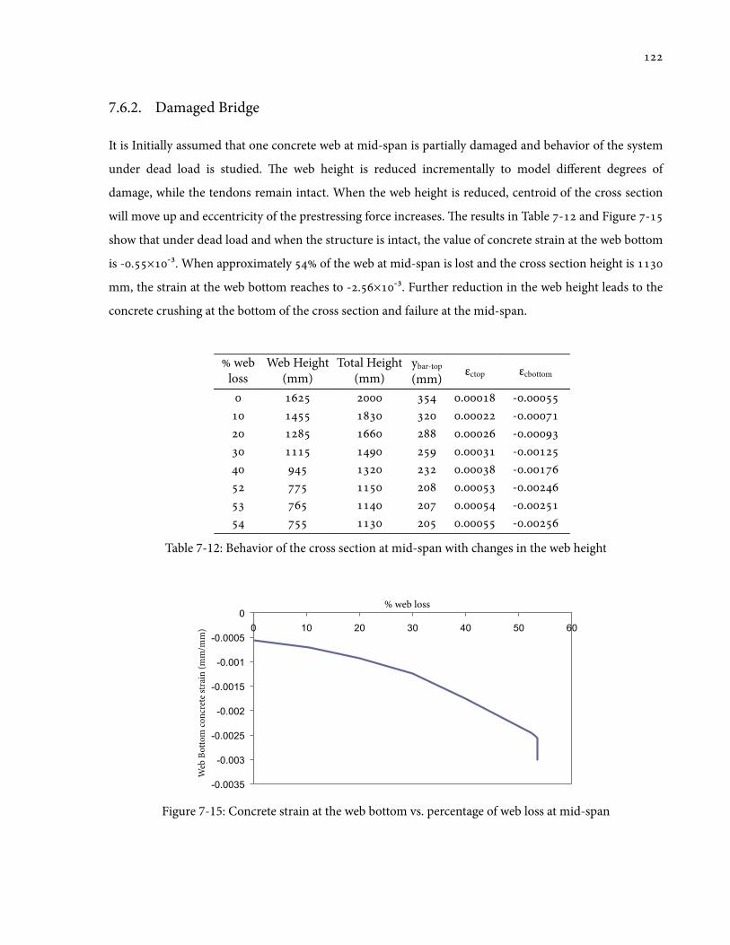
7.6.2. Damaged Bridge
It is Initially assumed that one concrete web at mid-span is partially damaged and behavior of the system
under dead load is studied. e web height is reduced incrementally to model different degrees of
damage, while the tendons remain intact. When the web height is reduced, centroid of the cross section
will move up and eccentricity of the prestressing force increases. e results in Table - and Figure -
show that under dead load and when the structure is intact, the value of concrete strain at the web bottom
is -.×3. When approximately of the web at mid-span is lost and the cross section height is
mm, the strain at the web bottom reaches to -.×3. Further reduction in the web height leads to the
concrete crushing at the bottom of the cross section and failure at the mid-span.
webloss
Web Height(mm)
Total Height(mm)
ybar-top
(mm) εctop εcbottom
. -. . -. . -. . -. . -. . -. . -. . -.
Table 7-12: Behavior of the cross section at mid-span with changes in the web height
Figure 7-15: Concrete strain at the web bottom vs. percentage of web loss at mid-span
-0.0035
-0.003
-0.0025
-0.002
-0.0015
-0.001
-0.0005
0
0 10 20 30 40 50 60
Web
Bot
tom
conc
rete
stra
in (m
m/m
m)
% web loss
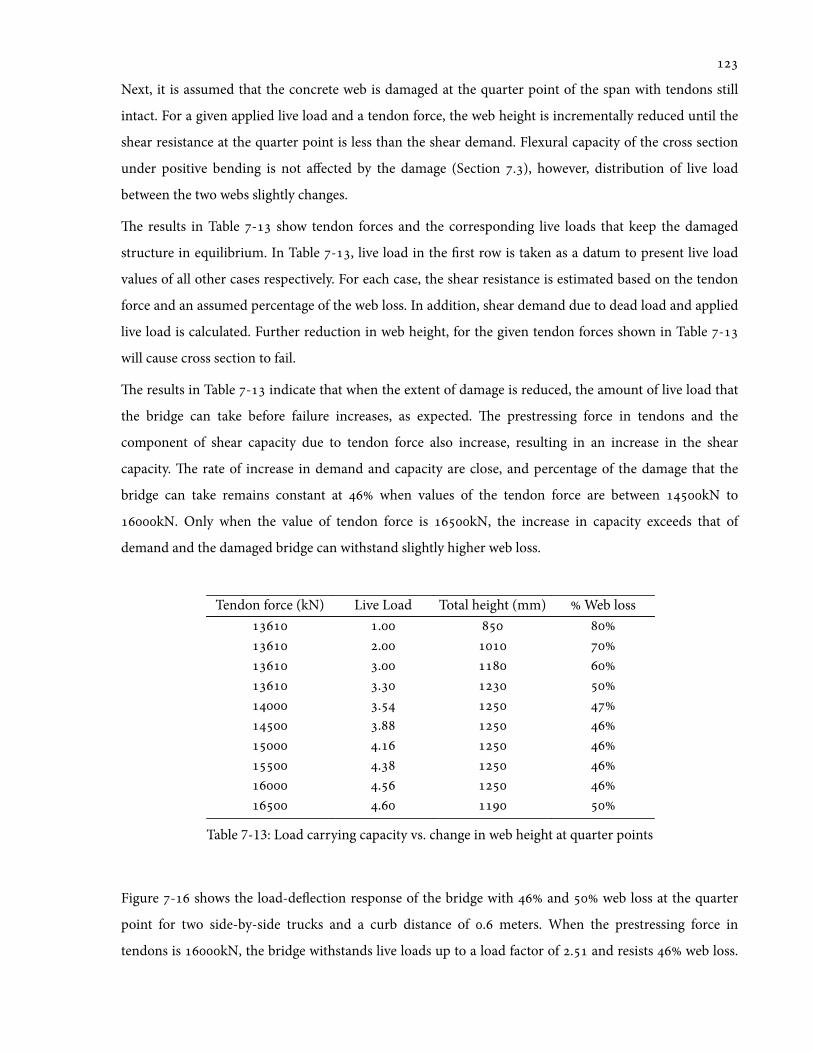
Next, it is assumed that the concrete web is damaged at the quarter point of the span with tendons still
intact. For a given applied live load and a tendon force, the web height is incrementally reduced until the
shear resistance at the quarter point is less than the shear demand. Flexural capacity of the cross section
under positive bending is not affected by the damage (Section .), however, distribution of live load
between the two webs slightly changes.
e results in Table - show tendon forces and the corresponding live loads that keep the damaged
structure in equilibrium. In Table -, live load in the 'rst row is taken as a datum to present live load
values of all other cases respectively. For each case, the shear resistance is estimated based on the tendon
force and an assumed percentage of the web loss. In addition, shear demand due to dead load and applied
live load is calculated. Further reduction in web height, for the given tendon forces shown in Table -
will cause cross section to fail.
e results in Table - indicate that when the extent of damage is reduced, the amount of live load that
the bridge can take before failure increases, as expected. e prestressing force in tendons and the
component of shear capacity due to tendon force also increase, resulting in an increase in the shear
capacity. e rate of increase in demand and capacity are close, and percentage of the damage that the
bridge can take remains constant at when values of the tendon force are between kN to
kN. Only when the value of tendon force is kN, the increase in capacity exceeds that of
demand and the damaged bridge can withstand slightly higher web loss.
Tendon force (kN) Live Load Total height (mm) Web loss . . . . . . . . . .
Table 7-13: Load carrying capacity vs. change in web height at quarter points
Figure - shows the load-de1ection response of the bridge with and web loss at the quarter
point for two side-by-side trucks and a curb distance of . meters. When the prestressing force in
tendons is kN, the bridge withstands live loads up to a load factor of . and resists web loss.
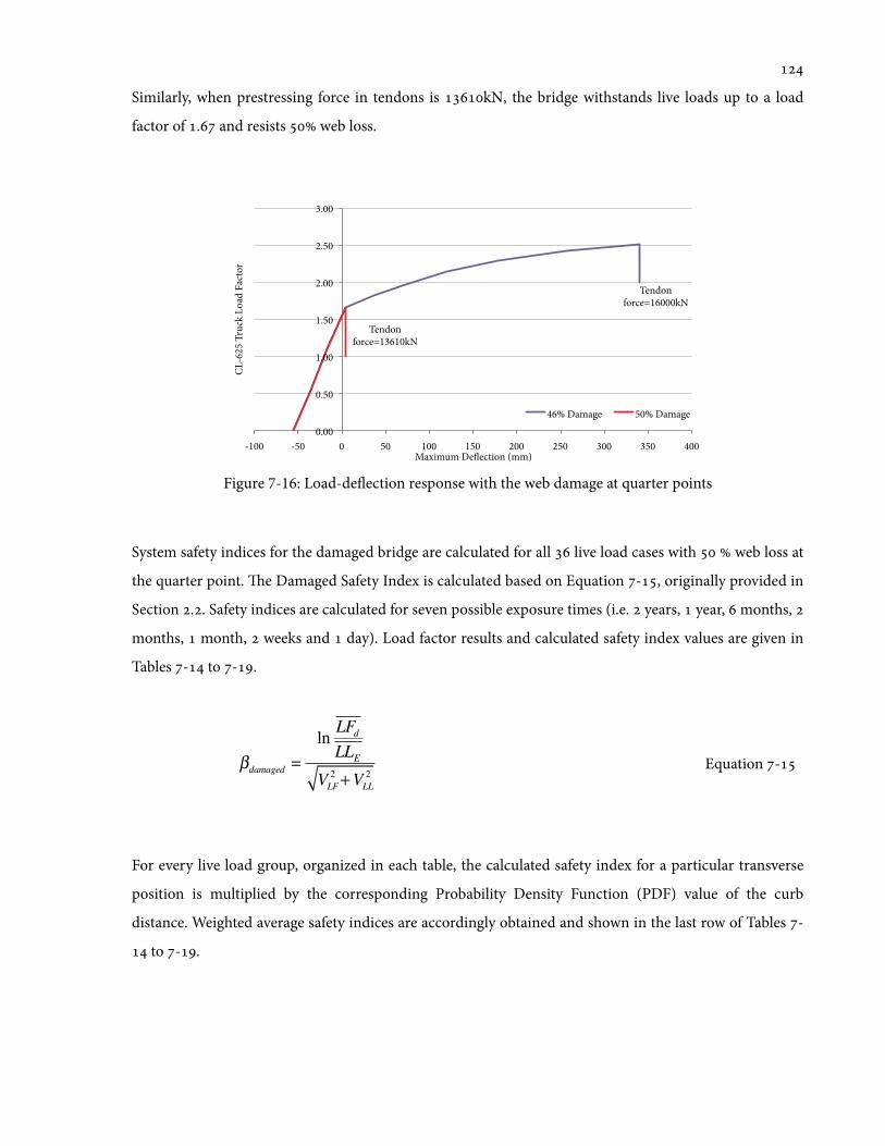
Similarly, when prestressing force in tendons is kN, the bridge withstands live loads up to a load
factor of . and resists web loss.
Figure 7-16: Load-de1ection response with the web damage at quarter points
System safety indices for the damaged bridge are calculated for all live load cases with web loss at
the quarter point. e Damaged Safety Index is calculated based on Equation -, originally provided in
Section .. Safety indices are calculated for seven possible exposure times (i.e. years, year, months,
months, month, weeks and day). Load factor results and calculated safety index values are given in
Tables - to -.
βdamaged =ln LFdLLE
VLF2 +VLL
2Equation -
For every live load group, organized in each table, the calculated safety index for a particular transverse
position is multiplied by the corresponding Probability Density Function (PDF) value of the curb
distance. Weighted average safety indices are accordingly obtained and shown in the last row of Tables -
to -.
Tendon force=16000kN
Tendon force=13610kN
0.00
0.50
1.00
1.50
2.00
2.50
3.00
-100 -50 0 50 100 150 200 250 300 350 400
CL-6
25 T
ruck
Loa
d Fa
ctor
Maximum De!ection (mm)
46% Damage 50% Damage
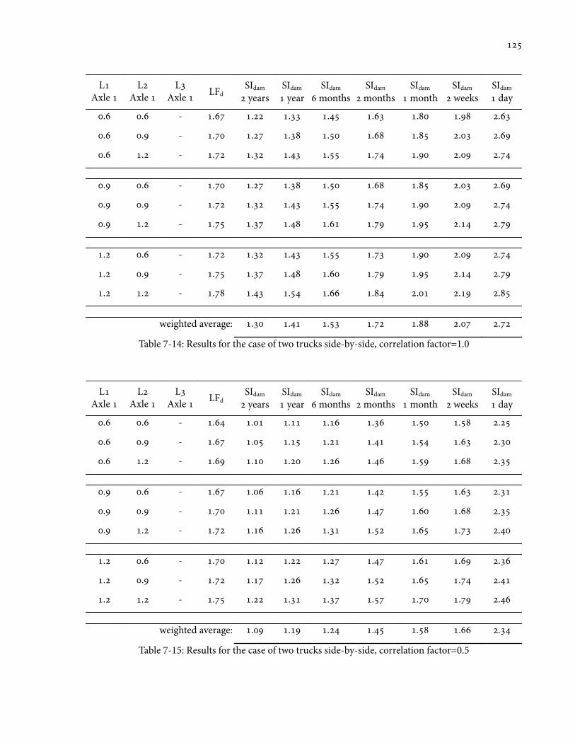
LAxle
LAxle
LAxle LFd
SIdam
yearsSIdam
yearSIdam
monthsSIdam
monthsSIdam
monthSIdam
weeksSIdam
day
. . - . . . . . . . .
. . - . . . . . . . .
. . - . . . . . . . .
. . - . . . . . . . .
. . - . . . . . . . .
. . - . . . . . . . .
. . - . . . . . . . .
. . - . . . . . . . .
. . - . . . . . . . .
weighted average: . . . . . . .
Table 7-14: Results for the case of two trucks side-by-side, correlation factor=1.0
LAxle
LAxle
LAxle LFd
SIdam
yearsSIdam
yearSIdam
monthsSIdam
monthsSIdam
monthSIdam
weeksSIdam
day
. . - . . . . . . . .
. . - . . . . . . . .
. . - . . . . . . . .
. . - . . . . . . . .
. . - . . . . . . . .
. . - . . . . . . . .
. . - . . . . . . . .
. . - . . . . . . . .
. . - . . . . . . . .
weighted average: . . . . . . .
Table 7-15: Results for the case of two trucks side-by-side, correlation factor=0.5
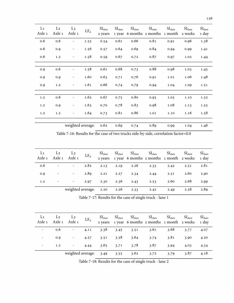
LAxle
LAxle
LAxle LFd
SIdam
yearsSIdam
yearSIdam
monthsSIdam
monthsSIdam
monthSIdam
weeksSIdam
day
. . - . . . . . . . .
. . - . . . . . . . .
. . - . . . . . . . .
. . - . . . . . . . .
. . - . . . . . . . .
. . - . . . . . . . .
. . - . . . . . . . .
. . - . . . . . . . .
. . - . . . . . . . .
weighted average: . . . . . . .
Table 7-16: Results for the case of two trucks side-by-side, correlation factor=0.0
LAxle
LAxle
LAxle LFd
SIdam
yearsSIdam
yearSIdam
monthsSIdam
monthsSIdam
monthSIdam
weeksSIdam
day
. - - . . . . . . . .
. - - . . . . . . . .
. - - . . . . . . . .
weighted average: . . . . . . .
Table 7-17: Results for the case of single truck - lane 1
LAxle
LAxle
LAxle LFd
SIdam
yearsSIdam
yearSIdam
monthsSIdam
monthsSIdam
monthSIdam
weeksSIdam
day
- . - . . . . . . . .
- . - . . . . . . . .
- . - . . . . . . . .
weighted average: . . . . . . .
Table 7-18: Results for the case of single truck - lane 2
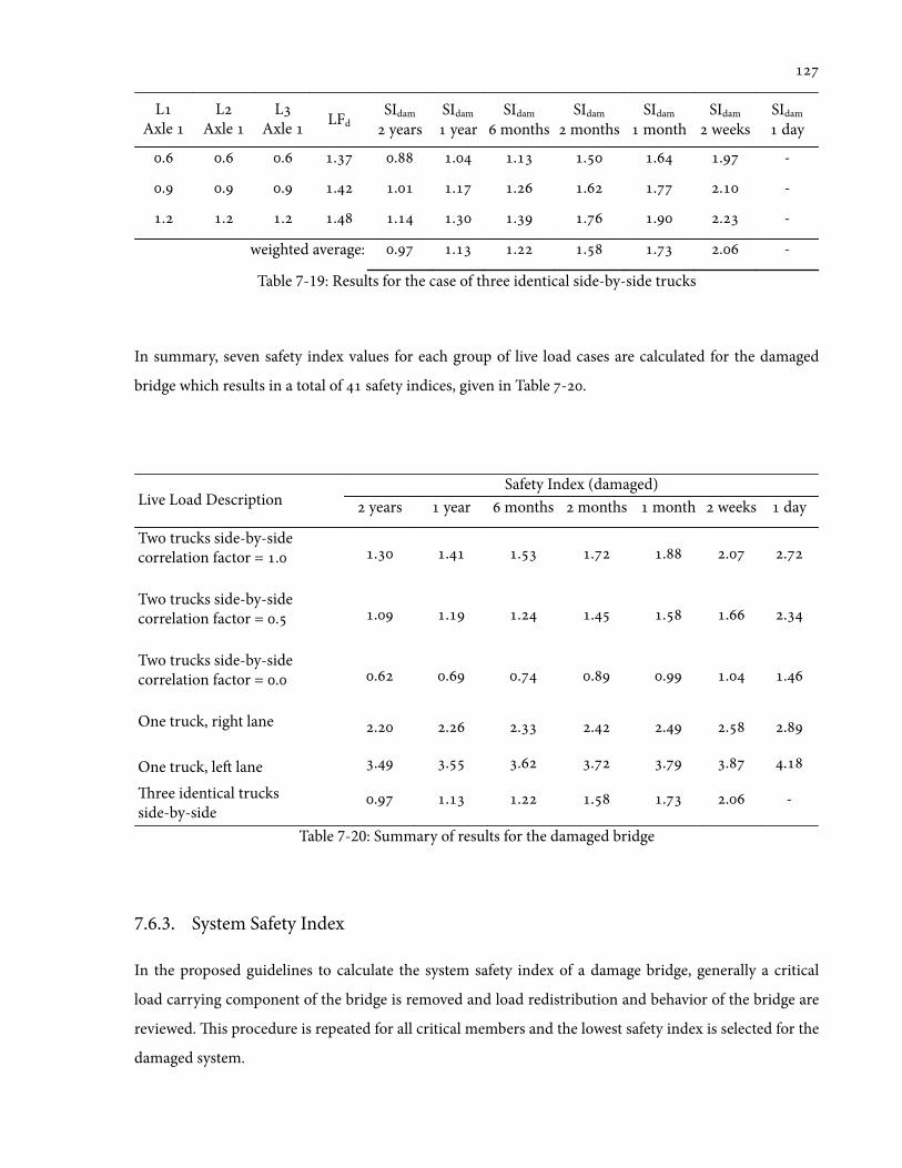
LAxle
LAxle
LAxle LFd
SIdam
yearsSIdam
yearSIdam
monthsSIdam
monthsSIdam
monthSIdam
weeksSIdam
day
. . . . . . . . . . -
. . . . . . . . . . -
. . . . . . . . . . -
weighted average: . . . . . . -
Table 7-19: Results for the case of three identical side-by-side trucks
In summary, seven safety index values for each group of live load cases are calculated for the damaged
bridge which results in a total of safety indices, given in Table -.
Live Load DescriptionSafety Index (damaged)
years year months months month weeks day
Two trucks side-by-side correlation factor = . . . . . . . .
Two trucks side-by-sidecorrelation factor = . . . . . . . .
Two trucks side-by-sidecorrelation factor = . . . . . . . .
One truck, right lane . . . . . . .
One truck, le lane . . . . . . .
ree identical trucks side-by-side
. . . . . . -
Table 7-20: Summary of results for the damaged bridge
7.6.3. System Safety Index
In the proposed guidelines to calculate the system safety index of a damage bridge, generally a critical
load carrying component of the bridge is removed and load redistribution and behavior of the bridge are
reviewed. is procedure is repeated for all critical members and the lowest safety index is selected for the
damaged system.
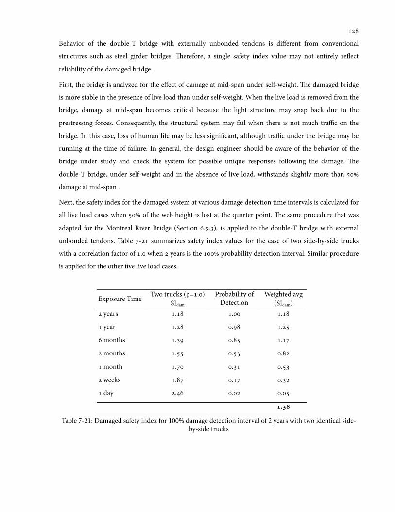
Behavior of the double-T bridge with externally unbonded tendons is different from conventional
structures such as steel girder bridges. erefore, a single safety index value may not entirely re1ect
reliability of the damaged bridge.
First, the bridge is analyzed for the effect of damage at mid-span under self-weight. e damaged bridge
is more stable in the presence of live load than under self-weight. When the live load is removed from the
bridge, damage at mid-span becomes critical because the light structure may snap back due to the
prestressing forces. Consequently, the structural system may fail when there is not much traffic on the
bridge. In this case, loss of human life may be less signi'cant, although traffic under the bridge may be
running at the time of failure. In general, the design engineer should be aware of the behavior of the
bridge under study and check the system for possible unique responses following the damage. e
double-T bridge, under self-weight and in the absence of live load, withstands slightly more than
damage at mid-span .
Next, the safety index for the damaged system at various damage detection time intervals is calculated for
all live load cases when of the web height is lost at the quarter point. e same procedure that was
adapted for the Montreal River Bridge (Section ..), is applied to the double-T bridge with external
unbonded tendons. Table - summarizes safety index values for the case of two side-by-side trucks
with a correlation factor of . when years is the probability detection interval. Similar procedure
is applied for the other 've live load cases.
Exposure Time Two trucks (ρ=.)SIdam
Probability ofDetection
Weighted avg(SIdam)
years . . .
year . . .
months . . .
months . . .
month . . .
weeks . . .
day . . .
.
Table 7-21: Damaged safety index for 100% damage detection interval of 2 years with two identical side-by-side trucks
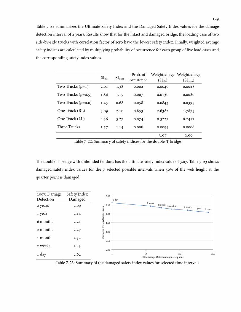
Table - summarizes the Ultimate Safety Index and the Damaged Safety Index values for the damage
detection interval of years. Results show that for the intact and damaged bridge, the loading case of two
side-by-side trucks with correlation factor of zero have the lowest safety index. Finally, weighted average
safety indices are calculated by multiplying probability of occurrence for each group of live load cases and
the corresponding safety index values.
SIult SIdamProb. of
occurenceWeighted avg
(SIult)Weighted avg
(SIdam)Two Trucks (ρ=) . . . . .
Two Trucks (ρ=.) . . . . .
Two Trucks (ρ=.) . . . . .
One Truck (RL) . . . . .
One Truck (LL) . . . . .
ree Trucks . . . . .
. .Table 7-22: Summary of safety indices for the double-T bridge
e double-T bridge with unbonded tendons has the ultimate safety index value of .. Table - shows
damaged safety index values for the selected possible intervals when of the web height at the
quarter point is damaged.
Damage Detection
Safety IndexDamaged
2 years 1 year 6 monts 2 months 1 month 2 weeks 1 day
!"!!#
!"$!#
%"!!#
%"$!#
&"!!#
&"$!#
'"!!#
%# %!# %!!# %!!!#
Dam
aged
Sys
tem
Saf
ety
Inde
x
100% Damage Detection (days) - Log scale
years .
year .
months .
months .
month .
weeks .
day .
Table 7-23: Summary of the damaged safety index values for selected time intervals
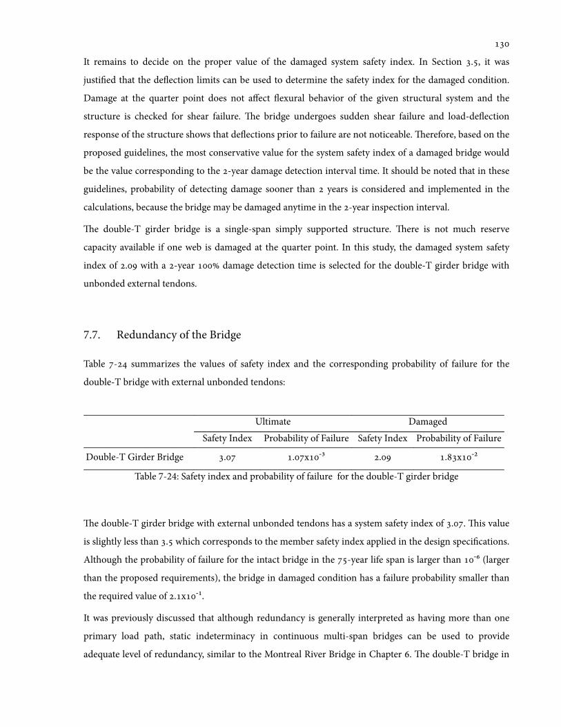
It remains to decide on the proper value of the damaged system safety index. In Section ., it was
justi'ed that the de1ection limits can be used to determine the safety index for the damaged condition.
Damage at the quarter point does not affect 1exural behavior of the given structural system and the
structure is checked for shear failure. e bridge undergoes sudden shear failure and load-de1ection
response of the structure shows that de1ections prior to failure are not noticeable. erefore, based on the
proposed guidelines, the most conservative value for the system safety index of a damaged bridge would
be the value corresponding to the -year damage detection interval time. It should be noted that in these
guidelines, probability of detecting damage sooner than years is considered and implemented in the
calculations, because the bridge may be damaged anytime in the -year inspection interval.
e double-T girder bridge is a single-span simply supported structure. ere is not much reserve
capacity available if one web is damaged at the quarter point. In this study, the damaged system safety
index of . with a -year damage detection time is selected for the double-T girder bridge with
unbonded external tendons.
7.7. Redundancy of the Bridge
Table - summarizes the values of safety index and the corresponding probability of failure for the
double-T bridge with external unbonded tendons:
Ultimate Damaged
Safety Index Probability of Failure Safety Index Probability of Failure
Double-T Girder Bridge . .x3 . .x2
Table 7-24: Safety index and probability of failure for the double-T girder bridge
e double-T girder bridge with external unbonded tendons has a system safety index of .. is value
is slightly less than . which corresponds to the member safety index applied in the design speci'cations.
Although the probability of failure for the intact bridge in the -year life span is larger than ⁶ (larger
than the proposed requirements), the bridge in damaged condition has a failure probability smaller than
the required value of .x1.
It was previously discussed that although redundancy is generally interpreted as having more than one
primary load path, static indeterminacy in continuous multi-span bridges can be used to provide
adequate level of redundancy, similar to the Montreal River Bridge in Chapter . e double-T bridge in

this chapter is a simply supported single span structure with a system safety index that is close to the
member safety index as expected. However, given the structural system, the bridge is robust under
various damage conditions. In case of the web loss at mid-span, the prestressing force may cause
considerable negative bending. If such behavior is detected, the prestressing force in tendons can be
relaxed accordingly to avoid failure until the bridge is closed to traffic and proper measures are taken. e
bridge with of web loss at the quarter point can also withstand reasonable traffic loads and the -year
failure probability in damaged conditions satis'es the imposed requirements.
Also, it should be noted that in the reliability index formula, the resistance coefficient of variation for the
prestressed concrete members under 1exure is . whereas for composite steel girders under 1exure is
. (these values are based on Table -, Page ). is implies that, under 1exure, for the same level of
load carrying capacity, the double-T girder bridge has a higher system safety index than the Montreal
River Bridge.
Finally, it can be concluded that application of double-T girder bridges with external unbonded tendons
can be used to achieve high intrinsic robustness in design of bridges while minimizing material
consumption and economic premium.

Chapter 8
Summary, Conclusions and Recommendations for Future Work
8.1. Summary
e purpose of this study, as explained in the opening chapter, was to demonstrate that two-girder or
two-web structural systems can be employed to design efficient and safe bridges with an adequate level of
redundancy. e two major research objectives of this thesis were () to develop a comprehensive
procedure to assess redundancy of bridges and examine the ability of a damaged bridge to take traffic
loads until closure and () to apply the developed procedure to two distinct bridges to show that two-
girder or two-web structures can provide acceptable level of safety.
e 'rst objective is accomplished through the use of the NCHRP Report and current available
statistical data on traffic loads, described in Chapters and . In the developed procedure, the system
safety index is calculated for a bridge at intact and damaged conditions. e ultimate capacity of a bridge
in both intact and damaged conditions are compared to the expected traffic (live load) on the structure.
At intact condition, the bridge is evaluated against -year loading event which is the intended design life
time of the structure. At damaged conditions, de1ection limits are incorporated to determine the time
interval that the de1ections become detectable and the bridge is closed to traffic. In case of damaged
bridges, generally, the guidelines are applied to the structure with a main load carrying member removed
and the procedure is repeated if more than one critical member is identi'ed.

Based on the calculated safety indices, corresponding values of the probability of failure are calculated
and compared with the relevant acceptable margin. As part of developing the procedure, current
literature on the optimum value of failure probability for a structure is studied in Chapter and the
decision is made on an acceptable level of redundancy. Given the limitations of the available guidelines, it
is decided that the probability of failure for an intact bridge in a -year life span should be smaller than
⁶ while the bridge in damaged conditions should have a maximum probability of failure of .x1 for
the relevant time interval before closure.
e second objective is accomplished through application of the procedure that was developed, on two
distinct bridge concepts: 'rst, the Montreal River Bridge concept with twin steel girders in Chapter and
second, the double-T girder bridge concept with external unbonded tendons in Chapter .
8.2. Conclusions
e conclusions drawn from this research can be summarized into two categories: () e general
conclusion on the developed analytical procedure for the evaluation of a bridge with regard to
redundancy and () the speci'c conclusions on safety of bridges with two-girder or two-web structural
systems.
() e developed procedure is applicable to all bridge structural systems and it is intended to
formulate safety indices to re1ect behavior of bridges in both intact and damaged conditions
under possible traffic loadings over time. e proposed guidelines are simple enough to be
adapted by engineers in practice to evaluate reliability of existing or new bridges. e work
involves computation of a safety index for a number of loading events and incorporates
probability concepts at different stages. A spreadsheet can be created to organize and include all
loading events and the corresponding probability values. erefore, it only remains to perform
nonlinear structural analysis and evaluate behavior of intact and damaged bridges for possible
truck positions at ultimate state. e developed procedure is summarized as a set of step-by-
step guidelines in Chapter .
() e reliability of the Montreal River Bridge concept, a twin steel girder with composite deck
slab, shows that two-girder bridges should not necessarily be classi'ed as non-redundant
structures. One way to create redundancy in a bridge, is to provide more than one primary load

path so that if a component fails, load is carried through another load path. is is the reason
for multi-girder bridges to be common in North America; however, provision of multiple
girders is not the only way to ensure redundancy. In the three-span Montreal River Bridge, the
static indeterminacy in continuous girders helps redistribute the applied load aer one girder is
damaged and results show that the bridge ful'lls all the imposed requirements to be a
redundant structure.
e reliability analysis of the double-T girder bridge concept with external unbonded tendons
shows that the structural system can exhibit high intrinsic robustness. e simply supported
structure with two webs has an intact safety index value close to the member safety factor, but
the damaged structure withstands the expected traffic and satis'es the required minimum
probability of failure. is concept can be extended to multi-span structures in which the static
indeterminacy considerably increases the redundancy at both intact and damaged conditions.
In conclusion, this thesis demonstrates that two-girder or two-web structural systems can be employed to
design bridges with an acceptable level of redundancy to ensure safety. e 'rst contribution of this thesis
is the generalization of current available knowledge on the reliability analysis of bridges to quantify
redundancy. is includes a comprehensive live load model that incorporates probabilistic characteristics
of loading events and provides a more realistic safety index values for a bridge. e second contribution
of this thesis is the implementation of the developed procedure to validate two-girder steel or two-web
concrete structural systems as viable and safe options for design of bridges.
8.3. Recommendations for Future Work
Although the proposed procedure is reasonably developed and applied to bridge concepts, certain
assumptions were made to account for current limitations. e future research work can be performed in
the following directions:
• e Live load model used in this study is based on current available literature and the
primary statistics of traffic on bridges is based on the data gathered in Ontario during late
s. e allowable truck weights have been increased over time and statistics of truck
traffic, their weight and accuracy of current live load model should be examined.
• e Live load model used in this study includes single and multi-lane loading events.
Comprehensive statistics for single loading events are available, but solid information or load

modeling on multi-vehicle traffic events on bridges is rare and hard to 'nd. Attempts have
been made to employ probability concepts and write computer codes that generate possible
loading events on a bridge. Application of these computer codes are generally complex and
hard to implement, but they can be used to develop the required statistics for a live load
model similar to what was used in this thesis. is way, the procedure would be made simple
enough to be applicable for engineers in practice.
• Contrary to previous guidelines, -year inspection interval is not selected as the exposure
time for the damaged bridges. In this study, damage detection time is selected based on the
behavior of bridges and de1ections aer component failure. is way a more realistic safety
index is calculated. However, available de1ection limits are based on experiments performed
on structural elements in general and are not speci'cally derived for bridges. ese limits
depend on the viewing angle of the observer; therefore, location of the bridge and its setting
in1uence the applicability of the de1ection limits. ese limits should be further studied and
in cases that their application cannot be justi'ed, an alternative procedure should be
proposed and the guideline for damage detection time should be improved.
• For the purpose of this thesis, the acceptable values of probability of failure are determined
based on the previous research on the subject. Available literature recognizes that an
appropriate value for the probability of failure should be in line with the expectations of
society as well as results of cost-bene't analysis to achieve an acceptable level of safety.
Currently, a wide range of guidelines are available but they generally fail to account for both
economical and societal aspects of safety simultaneously. While it is easier to decide on an
optimum economical value for probability of failure by adjusting quality and quantity of
materials, it is certainly not an easy task to incorporate consequences of failure at the society
level and further research is needed to obtain de'nite limiting values for the acceptable
probability of failure.
• Finally, this thesis mainly focused on reliability analysis of bridges to quantify redundancy of
structural systems. is is the 'rst step to develop a complete set of guidelines to assess
robustness of bridge structural systems in a broader scope. Redundancy in a structural
system is one way to improve robustness of structures. In bridges with large number of spans,
aer damage at a critical component of a given span, not only the bridge should withstand
the regular traffic, but it is also desirable to limit the extend of damage to the given span or a
few of nearby spans, in other words avoid progressive collapse. erefore, acceptable extent of
damage and provisions to prevent progressive collapse should be integrated with the

guidelines on redundancy of bridges. If such guidelines are developed and implemented in
design codes, structures can be designed at the system level as opposed to the component
level. is way both structural efficiency and safety can be ensured.

References:
AASHTO. 2004. AASHTO LRFD Bridge Design Specifications. SI Units. 3rd ed. Washington,
DC.
AASHTO. 2002. AASHTO Specifications for Highway Bridges. SI Units. 17th ed. Washington,
DC.
Agarwal, J. England, J and Blockley, D. 2006. “Vulnerability Analysis of Structures”.
Structural Engineering International. 2:124-128.
Alkhairi, F.M. and Naaman, A.E. 1993. “Analysis of Beams Prestressed With Unbonded
Internal Or External Tendons”. Journal of Structural Engineering. 119:2680-700.
CEN: European Committee for Standardization. 1996. pr. EN1991-1-7. Eurocode 1: General
Actions - Accidental Actions. CEN. Brussels, Belgium.
CEN: European Committee for Standardization. 2005. pr. EN1993. Eurocode 3: Design of Steel
Structures. CEN. Brussels, Belgium.
CSA: Canadian Standards Association. 2006a. CAN/CSA-S6-06: Canadian Highway Bridge
Design Code. CSA, Mississauga, Ontario.
CISC: Canadian Institute of Steel Construction. 2004. Handbook of Steel Construction. CISC.
Eighth Edition.

Chatfield, C. 1995. Statistics for Technology (a Course in Applied Statistics). Chapman & Hall/
CRC.
Chiou, J.S. Yang, H.H. and Chen, C.H. 2009. “Use of Plastic Hinge Model in Nonlinear
Pushover Analysis of a Pile”. Journal of Geotechnical and Geoenvironmental Engineering.
September.
Computer and Structures Inc. 2006. SAP2000 Linear and nonlinear static and dynamic analysis
and design of three dimensional structures. Berkeley, California.
Cordahi, I.A. 2006. “Reliability of Corroded Steel Bridge Girder”. Department of Civil and
Environmental Engineering. Massachusetts Institute of Technology. Master of Engineering.
Diamantidis, D. 2008. “Background Documents on Risk Assessment in Engineering: Document
No. 3, Risk Acceptable Criteria”. Joint Committee of Structural Safety (JCSS).
Duckett, W. 2004. “Risk Analysis and the Acceptable Probability of Failure.”. IABSE
Colloquium: Designing for the consequences of hazards.
Eamon, C.D. and Nowak, A.S. 2004. “Effect of Secondary Elements on Bridge Structural
System Reliability Considering Moment Capacity”. Structural Safety. 26:305-27.
FHWA: Federal Highway Administration. 2006. “LRFD Steel Girder Superstructure Bridge
Designer's Guide”. US Department of Transportation. <http://www.fhwa.dot.gov/bridge/lrfd/
us_ds1.htm >
Galambos, T. V. and Ellingwood, B. 1986. “Serviceability Limit States: Deflection”. Journal of
Structural Engineering. 112:67-84.

Galambos, T.V., Leon, R.T, French, C.W., Barker, M. and Dishongh, B. 1993. “Inelastic Rating
Procedures for Steel Beam and Girder Bridges”. NCHRP Report 352.
Gauvreau, P. 1992. “Load Tests of Concrete Girders With Unbonded Tendons”. Institute of
Structural Engineering. Swiss Federal Institute of Technology. Report No. 194. Basel, Boston,
Berlin: Birkhäuser Verlag.
Gauvreau, P. 1993. “Ultimate Limit State of Concrete Girders Prestressed with Unbonded
Tendons”. Institute of Structural Engineering. Swiss Federal Institute of Technology. Report
No. 198. Basel, Boston, Berlin: Birkhäuser Verlag.
Ghosn, M. and Moses, F. 1998. “Redundancy in Highway Bridge Superstructures”. NCHRP
Report 406. Transportation Research Board - National Research Council. Washington, D.C.
Gulvanessian, H. and Vrouwenvelder, T. 2006. “Robustness and the Eurocodes”. Structural
Engineering International. 2:167-171.
Guzda, M., Bhattacharya, B. and Mertz, D.R. 2007. “Probabilistic Characterization of Live
Load Using Visual Counts and in-Service Strain Monitoring”. Journal of Bridge Engineering.
Jan/Feb.:130-4.
Haldar, A. and Mahadevan S. 1999. Probability, Reliability, and Statistical Methods in
Engineering Design. John Wiley & Sons Inc.
IABSE: International Association for Bridge and Structural Engineering. 1993. “Ship collision
with bridges – the interaction between vessel traffic and bridge structures.” Structural
Engineering Documents.

Laane, A. and Lebet. J.P. 2005. “Available Rotation Capacity of Composite Bridge Plate
Girders Under Negative Moment and Shear.” Journal of Constructional Steel Research .
61:305-327.
Li, E. Y. 2010. “Bridge System With Precast Concrete Double-T Girder and External Unbonded
Post-Tensioning”. Department of Civil Engineering. University of Toronto. Master of Applied
Science.
MacGregor, J.G. 1976. “Safety and Limit States Design for Reinforced Concrete”. Canadian
Journal of Civil Engineering. 4:484-513.
Marchand, J. and Mitchell, D. 2007. Rapport sur les causes technique de l'effondrement du
viaduc de la Concorde - Rapport principal.
Melchers, R.E. 1999. Structural Reliability Analysis and Prediction. John Wiley & Sons Inc.
Menn, C. 1990. Prestressed Concrete Bridges. Birkhäuser Verlag, Basel, Switzerland.
Mermigas, k. 2007. “Economic Design of a Steel Girder Bridge, Comparison between four
girder and twin girder designs”. Department of Civil Engineering. University of Toronto.
Internal Report.
MN/DOT: Minneapolis Department of Transportation. 2007. Fatigue Evaluation and
Redundancy Analysis: I-35W over Mississippi River.
Moses, F. 2001. “Calibration of Load Factors for LRFD Bridge Evaluation”. NCHRP Report
454. Transportation Research Board - National Research Council. Washington, D.C.

NTSB: National Transportation Safety Board. 2007. Collapse of I-35W Highway Bridge
Minneapolis, Minnesota - Accident Report.
Nowak, A.S. 1995. “Calibration of LRFD Bridge Code”. Journal of Structural Engineering.
August: 1245:1251.
Nowak, A.S. 1999. “Calibration of LRFD Bridge Design Code”. NCHRP Report 368.
Transportation Research Board - National Research Council. Washington, D.C.
Nowak, A.S. 1994. “Load Model for Bridge Design Code”. Canadian Journal of Civil
Engineering. 21:36-49.
Nowak, A.S. and Szerszen, M. 2000. “Structural Reliability as Applied to Highway Bridges”.
Progress in Structural Engineering and Materials. 2:218-24.
Nowak, A.S. and Zhou, J. 1990. “System Reliability Models for Bridges.”. Structural Safety
7:247-54.
O’Brien, E.J. and Keogh, D.L. 1999. Bridge Deck Analysis. London: E & FN SPON.
OTUA: Office Technique pour l'Utilisation de l'Acier. 2004. INFOTUA: Thematic case study
No. 2: Steel Civil Engineering Structures; viaducts, bridges, footbridges.
Ressler, S.J. 1991. “Fatigue Reliability and Redundancy in Two-Girder Highway Bridges”.
Department of Civil Engineering. Lehigh University. Doctor of Philosophy
Ross, S.M. 2004. Introduction to Probability and Statistics for Engineers and Scientists. Elsvier
Academic Press.
Sétra: Service d'etudes sur les transports, les routes et leurs aménagements. 2010. Steel-
Concrete Composite Bridges - Sustainable Design Guide. Bangeux Cedex, France.
Starossek, U. 2006. “Progressive Collapse of Structures: Nomenclature and Procedures”.
IABSE, Structural Engineering International. 2:121-5.
Val, D.V. and Val, E.G. 2006. “Robustness of Frame Structures”. Journal of Structural
Engineering International. 2:108.
Vrouwenvelder, T. 2000. “Stochastic Modeling of Extreme Action Events in Structural
Engineering.”. Probabilistic Engineering Mechanics. 15:109-17.

Appendix A
Review of Statistical De'nitions

In this section some statistical de'nitions, that are used in this thesis, will be reviewed.
A histogram is a bar graph with bars placed adjacent to each other representing the frequency of data
points (Ross, ). For continuous random variables, with enough sample data, the bar intervals in the
histogram will be very small and histogram is turned into a smooth curve called the Probability Density
Function (PDF), shown in Figure A-. (Ross, )
Figure A-1: Normal Probability Density Function (PDF) of a Random Variable
In statistics, probability density function for a random variable X is de'ned as the function f(x) where for
any set B of real numbers:
P x ∈B{ } = f (x)dxB∫ for all real x ∈(−∞,+∞) Equation A-
Another important concept is the Cumulative Distribution Function (CDF) which shows the probability
that a random variable X takes on a value that is less than or equal to x (Ross, ). Mathematical
formulation for Cumulative Distribution Function is de'ned as the function F of a random variable X for
all real x ∈(−∞,+∞) :
F(x) = P X ≤ x{ } Equation A-
e variable in Figure A-, has an arithmetic average or mean x representing the peak of all data points
and σ x is the standard deviation that shows dispersion of data. Standard deviation for a set of data points
can be calculated as shown in Equation A-. Standard deviation to the power of two, σ 2x is called
variance.
13.6%13.6%
34.1%34.1%
Mean
std. dev. std. dev. std. dev.std. dev.
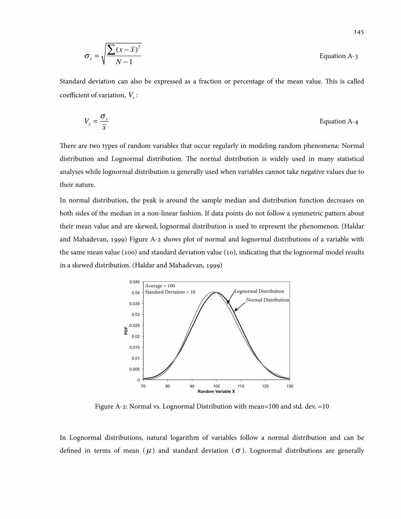
σ x =(x − x )2∑N −1
Equation A-
Standard deviation can also be expressed as a fraction or percentage of the mean value. is is called
coefficient of variation, Vx :
Vx =σ x
xEquation A-
ere are two types of random variables that occur regularly in modeling random phenomena: Normal
distribution and Lognormal distribution. e normal distribution is widely used in many statistical
analyses while lognormal distribution is generally used when variables cannot take negative values due to
their nature.
In normal distribution, the peak is around the sample median and distribution function decreases on
both sides of the median in a non-linear fashion. If data points do not follow a symmetric pattern about
their mean value and are skewed, lognormal distribution is used to represent the phenomenon. (Haldar
and Mahadevan, ) Figure A- shows plot of normal and lognormal distributions of a variable with
the same mean value () and standard deviation value (), indicating that the lognormal model results
in a skewed distribution. (Haldar and Mahadevan, )
Figure A-: Normal vs. Lognormal Distribution with mean=100 and std. dev. =10
In Lognormal distributions, natural logarithm of variables follow a normal distribution and can be
de'ned in terms of mean (µ ) and standard deviation (σ ). Lognormal distributions are generally
0
0.005
0.01
0.015
0.02
0.025
0.03
0.035
0.04
0.045
70 80 90 100 110 120 130
PD
F
Random Variable X
Lognormal DistributionNormal Distribution
Average = 100Standard Deviation = 10
expressed in terms of two parameters, λX and ς X , which are de'ned in terms of corresponding normal
distribution parameters shown in Equations A- and A-:
λx = E(ln x) = lnµx −12ζ 2x Equation A-
ζ 2x = Var(ln x) = ln 1+σ x
µx
⎛⎝⎜
⎞⎠⎟
2⎡
⎣⎢⎢
⎤
⎦⎥⎥= ln(1+Vx2 ) Equation A-
where E(X) is the expected value function of variable X and Var(X) is variance of variable X. Equation
A- de'nes the expected value function for variable X:
E X[ ] = xiP X = xi{ }i∑ Equation A-
is is “the weighted average of possible values that X can take, each value being weighted by the
probability that X assumes.” (Ross, )
e result of linear combination of two or more normally distributed variables is also a normal variable. If
A and B are independent random variables with means A and B , standard deviations σ A and σ B and
coefficient of variations VA and VB , the following holds true :(MacGregor, )
Let X = A − B (or X = A + B ) Equation A-
en X = A − B (or X = A + B ) Equation A-
And σ x = σ A2 +σ B
2 Equation A-
In this thesis N (A,σ A ) represents a normal variable with mean Ā and standard deviation σA where N
stands for normal distribution.
Based on properties of normal random variables, if X is a normal variable with mean µ and variance σ 2
then Y = αX + β is also a normal variable with mean αµ + β and variance α 2σ 2 . It follows that
random variable Z with probability density function that is de'ned in Equation A- is normal with
mean zero and variance one.
Z =X − µσ
Equation A-

Such a random variable Z has a Standard Normal Distribution. erefore probability density function of
X is obtained from the corresponding graph for Z by a stretch parallel to the z-axis, centre at origin and
scale-factor σ followed by a translation μ along the z-axis. is will allow to write any probability
expression of variable X in terms of variable Z shown in Equation A-.
P X < b{ } = P X − µσ
<b − µσ
⎧⎨⎩
⎫⎬⎭= Φ(b − µ
σ) Equation A-
It remains to compute cumulative distribution function Φ of a random variable. ere are commonly
available tables which tabulate Φ(x) for a wide range of nonnegative values of X, a table of Standard
Normal Probability is provided in Appendix B.

Appendix B
Standard Normal Probability Table
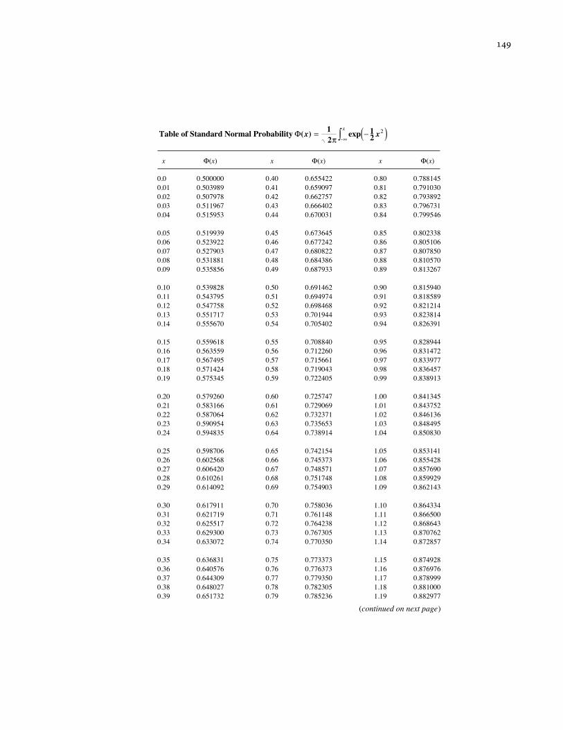
x !(x) x !(x) x !(x)
0.0 0.500000
0.01 0.503989
0.02 0.507978
0.03 0.511967
0.04 0.515953
0.05 0.519939
0.06 0.523922
0.07 0.527903
0.08 0.531881
0.09 0.535856
0.10 0.539828
0.11 0.543795
0.12 0.547758
0.13 0.551717
0.14 0.555670
0.15 0.559618
0.16 0.563559
0.17 0.567495
0.18 0.571424
0.19 0.575345
0.20 0.579260
0.21 0.583166
0.22 0.587064
0.23 0.590954
0.24 0.594835
0.25 0.598706
0.26 0.602568
0.27 0.606420
0.28 0.610261
0.29 0.614092
0.30 0.617911
0.31 0.621719
0.32 0.625517
0.33 0.629300
0.34 0.633072
0.35 0.636831
0.36 0.640576
0.37 0.644309
0.38 0.648027
0.39 0.651732
Table of Standard Normal Probability -
!( )1
2exp 1
2x x= "( )
#$%2
x
0.40 0.655422
0.41 0.659097
0.42 0.662757
0.43 0.666402
0.44 0.670031
0.45 0.673645
0.46 0.677242
0.47 0.680822
0.48 0.684386
0.49 0.687933
0.50 0.691462
0.51 0.694974
0.52 0.698468
0.53 0.701944
0.54 0.705402
0.55 0.708840
0.56 0.712260
0.57 0.715661
0.58 0.719043
0.59 0.722405
0.60 0.725747
0.61 0.729069
0.62 0.732371
0.63 0.735653
0.64 0.738914
0.65 0.742154
0.66 0.745373
0.67 0.748571
0.68 0.751748
0.69 0.754903
0.70 0.758036
0.71 0.761148
0.72 0.764238
0.73 0.767305
0.74 0.770350
0.75 0.773373
0.76 0.776373
0.77 0.779350
0.78 0.782305
0.79 0.785236
0.80 0.788145
0.81 0.791030
0.82 0.793892
0.83 0.796731
0.84 0.799546
0.85 0.802338
0.86 0.805106
0.87 0.807850
0.88 0.810570
0.89 0.813267
0.90 0.815940
0.91 0.818589
0.92 0.821214
0.93 0.823814
0.94 0.826391
0.95 0.828944
0.96 0.831472
0.97 0.833977
0.98 0.836457
0.99 0.838913
1.00 0.841345
1.01 0.843752
1.02 0.846136
1.03 0.848495
1.04 0.850830
1.05 0.853141
1.06 0.855428
1.07 0.857690
1.08 0.859929
1.09 0.862143
1.10 0.864334
1.11 0.866500
1.12 0.868643
1.13 0.870762
1.14 0.872857
1.15 0.874928
1.16 0.876976
1.17 0.878999
1.18 0.881000
1.19 0.882977
(continued on next page)
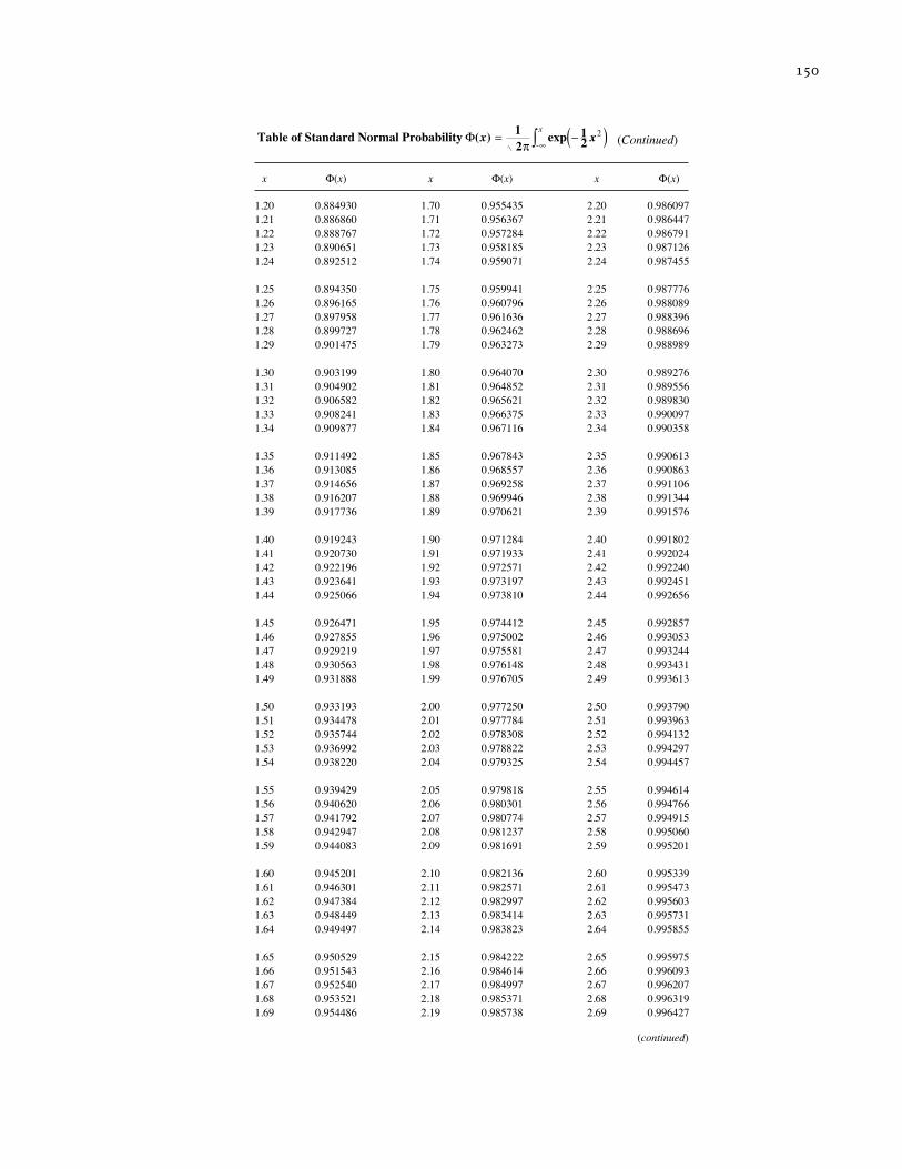
(Continued)
x !(x) x !(x) x !(x)
1.20 0.884930
1.21 0.886860
1.22 0.888767
1.23 0.890651
1.24 0.892512
1.25 0.894350
1.26 0.896165
1.27 0.897958
1.28 0.899727
1.29 0.901475
1.30 0.903199
1.31 0.904902
1.32 0.906582
1.33 0.908241
1.34 0.909877
1.35 0.911492
1.36 0.913085
1.37 0.914656
1.38 0.916207
1.39 0.917736
1.40 0.919243
1.41 0.920730
1.42 0.922196
1.43 0.923641
1.44 0.925066
1.45 0.926471
1.46 0.927855
1.47 0.929219
1.48 0.930563
1.49 0.931888
1.50 0.933193
1.51 0.934478
1.52 0.935744
1.53 0.936992
1.54 0.938220
1.55 0.939429
1.56 0.940620
1.57 0.941792
1.58 0.942947
1.59 0.944083
1.60 0.945201
1.61 0.946301
1.62 0.947384
1.63 0.948449
1.64 0.949497
1.65 0.950529
1.66 0.951543
1.67 0.952540
1.68 0.953521
1.69 0.954486
Table of Standard Normal Probability -
!( )1
2exp 1
2x x= "( )
#$%2
x
1.70 0.955435
1.71 0.956367
1.72 0.957284
1.73 0.958185
1.74 0.959071
1.75 0.959941
1.76 0.960796
1.77 0.961636
1.78 0.962462
1.79 0.963273
1.80 0.964070
1.81 0.964852
1.82 0.965621
1.83 0.966375
1.84 0.967116
1.85 0.967843
1.86 0.968557
1.87 0.969258
1.88 0.969946
1.89 0.970621
1.90 0.971284
1.91 0.971933
1.92 0.972571
1.93 0.973197
1.94 0.973810
1.95 0.974412
1.96 0.975002
1.97 0.975581
1.98 0.976148
1.99 0.976705
2.00 0.977250
2.01 0.977784
2.02 0.978308
2.03 0.978822
2.04 0.979325
2.05 0.979818
2.06 0.980301
2.07 0.980774
2.08 0.981237
2.09 0.981691
2.10 0.982136
2.11 0.982571
2.12 0.982997
2.13 0.983414
2.14 0.983823
2.15 0.984222
2.16 0.984614
2.17 0.984997
2.18 0.985371
2.19 0.985738
2.20 0.986097
2.21 0.986447
2.22 0.986791
2.23 0.987126
2.24 0.987455
2.25 0.987776
2.26 0.988089
2.27 0.988396
2.28 0.988696
2.29 0.988989
2.30 0.989276
2.31 0.989556
2.32 0.989830
2.33 0.990097
2.34 0.990358
2.35 0.990613
2.36 0.990863
2.37 0.991106
2.38 0.991344
2.39 0.991576
2.40 0.991802
2.41 0.992024
2.42 0.992240
2.43 0.992451
2.44 0.992656
2.45 0.992857
2.46 0.993053
2.47 0.993244
2.48 0.993431
2.49 0.993613
2.50 0.993790
2.51 0.993963
2.52 0.994132
2.53 0.994297
2.54 0.994457
2.55 0.994614
2.56 0.994766
2.57 0.994915
2.58 0.995060
2.59 0.995201
2.60 0.995339
2.61 0.995473
2.62 0.995603
2.63 0.995731
2.64 0.995855
2.65 0.995975
2.66 0.996093
2.67 0.996207
2.68 0.996319
2.69 0.996427
(continued)
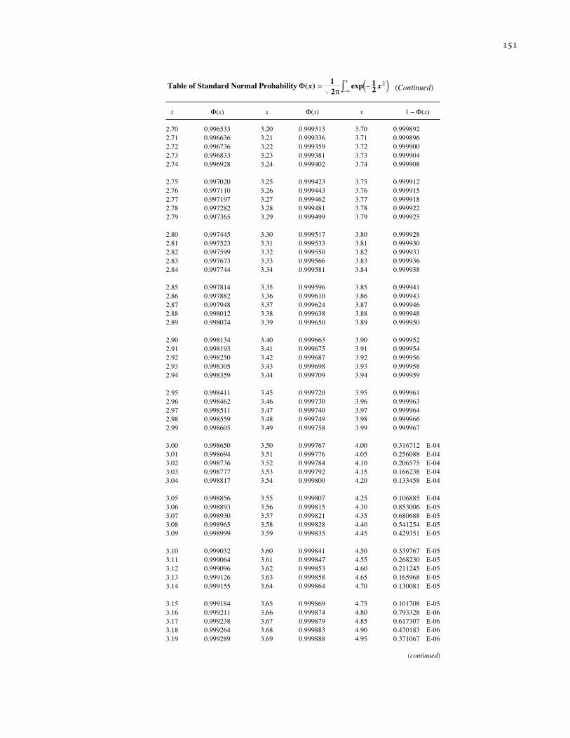
(continued)
(Continued)
x !(x) x !(x) x 1 " !(x)
2.70 0.996533
2.71 0.996636
2.72 0.996736
2.73 0.996833
2.74 0.996928
2.75 0.997020
2.76 0.997110
2.77 0.997197
2.78 0.997282
2.79 0.997365
2.80 0.997445
2.81 0.997523
2.82 0.997599
2.83 0.997673
2.84 0.997744
2.85 0.997814
2.86 0.997882
2.87 0.997948
2.88 0.998012
2.89 0.998074
2.90 0.998134
2.91 0.998193
2.92 0.998250
2.93 0.998305
2.94 0.998359
2.95 0.998411
2.96 0.998462
2.97 0.998511
2.98 0.998559
2.99 0.998605
3.00 0.998650
3.01 0.998694
3.02 0.998736
3.03 0.998777
3.04 0.998817
3.05 0.998856
3.06 0.998893
3.07 0.998930
3.08 0.998965
3.09 0.998999
3.10 0.999032
3.11 0.999064
3.12 0.999096
3.13 0.999126
3.14 0.999155
3.15 0.999184
3.16 0.999211
3.17 0.999238
3.18 0.999264
3.19 0.999289
Table of Standard Normal Probability -
!( )1
2exp 1
2x x= "( )
#$%2
x
3.20 0.999313
3.21 0.999336
3.22 0.999359
3.23 0.999381
3.24 0.999402
3.25 0.999423
3.26 0.999443
3.27 0.999462
3.28 0.999481
3.29 0.999499
3.30 0.999517
3.31 0.999533
3.32 0.999550
3.33 0.999566
3.34 0.999581
3.35 0.999596
3.36 0.999610
3.37 0.999624
3.38 0.999638
3.39 0.999650
3.40 0.999663
3.41 0.999675
3.42 0.999687
3.43 0.999698
3.44 0.999709
3.45 0.999720
3.46 0.999730
3.47 0.999740
3.48 0.999749
3.49 0.999758
3.50 0.999767
3.51 0.999776
3.52 0.999784
3.53 0.999792
3.54 0.999800
3.55 0.999807
3.56 0.999815
3.57 0.999821
3.58 0.999828
3.59 0.999835
3.60 0.999841
3.61 0.999847
3.62 0.999853
3.63 0.999858
3.64 0.999864
3.65 0.999869
3.66 0.999874
3.67 0.999879
3.68 0.999883
3.69 0.999888
3.70 0.999892
3.71 0.999896
3.72 0.999900
3.73 0.999904
3.74 0.999908
3.75 0.999912
3.76 0.999915
3.77 0.999918
3.78 0.999922
3.79 0.999925
3.80 0.999928
3.81 0.999930
3.82 0.999933
3.83 0.999936
3.84 0.999938
3.85 0.999941
3.86 0.999943
3.87 0.999946
3.88 0.999948
3.89 0.999950
3.90 0.999952
3.91 0.999954
3.92 0.999956
3.93 0.999958
3.94 0.999959
3.95 0.999961
3.96 0.999963
3.97 0.999964
3.98 0.999966
3.99 0.999967
4.00 0.316712 E-04
4.05 0.256088 E-04
4.10 0.206575 E-04
4.15 0.166238 E-04
4.20 0.133458 E-04
4.25 0.106885 E-04
4.30 0.853006 E-05
4.35 0.680688 E-05
4.40 0.541254 E-05
4.45 0.429351 E-05
4.50 0.339767 E-05
4.55 0.268230 E-05
4.60 0.211245 E-05
4.65 0.165968 E-05
4.70 0.130081 E-05
4.75 0.101708 E-05
4.80 0.793328 E-06
4.85 0.617307 E-06
4.90 0.470183 E-06
4.95 0.371067 E-06
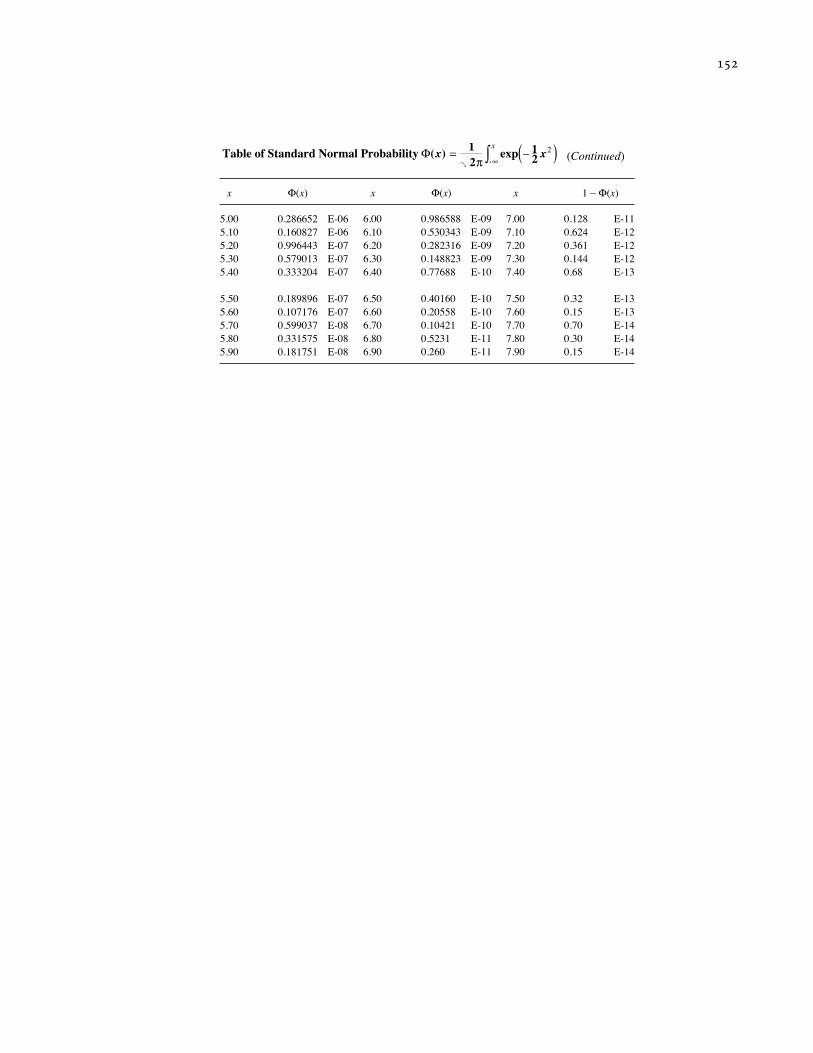
(Continued)
x !(x) x !(x) x 1 " !(x)
5.00 0.286652 E-06
5.10 0.160827 E-06
5.20 0.996443 E-07
5.30 0.579013 E-07
5.40 0.333204 E-07
5.50 0.189896 E-07
5.60 0.107176 E-07
5.70 0.599037 E-08
5.80 0.331575 E-08
5.90 0.181751 E-08
Table of Standard Normal Probability -
!( )1
2exp 1
2x x= "( )
#$%2
x
6.00 0.986588 E-09
6.10 0.530343 E-09
6.20 0.282316 E-09
6.30 0.148823 E-09
6.40 0.77688 E-10
6.50 0.40160 E-10
6.60 0.20558 E-10
6.70 0.10421 E-10
6.80 0.5231 E-11
6.90 0.260 E-11
7.00 0.128 E-11
7.10 0.624 E-12
7.20 0.361 E-12
7.30 0.144 E-12
7.40 0.68 E-13
7.50 0.32 E-13
7.60 0.15 E-13
7.70 0.70 E-14
7.80 0.30 E-14
7.90 0.15 E-14

Appendix C
e Montreal River Bridge - Details of Steel Girder Design
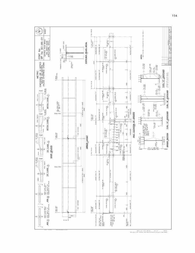

Appendix D
e Montreal River Bridge - SAP2000 Input File
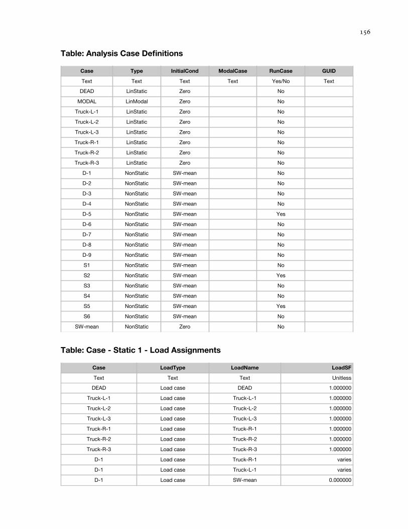
Table: Analysis Case Definitions
Case Type InitialCond ModalCase RunCase GUID
Text Text Text Text Yes/No Text
DEAD LinStatic Zero No
MODAL LinModal Zero No
Truck-L-1 LinStatic Zero No
Truck-L-2 LinStatic Zero No
Truck-L-3 LinStatic Zero No
Truck-R-1 LinStatic Zero No
Truck-R-2 LinStatic Zero No
Truck-R-3 LinStatic Zero No
D-1 NonStatic SW-mean No
D-2 NonStatic SW-mean No
D-3 NonStatic SW-mean No
D-4 NonStatic SW-mean No
D-5 NonStatic SW-mean Yes
D-6 NonStatic SW-mean No
D-7 NonStatic SW-mean No
D-8 NonStatic SW-mean No
D-9 NonStatic SW-mean No
S1 NonStatic SW-mean No
S2 NonStatic SW-mean Yes
S3 NonStatic SW-mean No
S4 NonStatic SW-mean No
S5 NonStatic SW-mean Yes
S6 NonStatic SW-mean No
SW-mean NonStatic Zero No
Table: Case - Static 1 - Load Assignments
Case LoadType LoadName LoadSF
Text Text Text Unitless
DEAD Load case DEAD 1.000000
Truck-L-1 Load case Truck-L-1 1.000000
Truck-L-2 Load case Truck-L-2 1.000000
Truck-L-3 Load case Truck-L-3 1.000000
Truck-R-1 Load case Truck-R-1 1.000000
Truck-R-2 Load case Truck-R-2 1.000000
Truck-R-3 Load case Truck-R-3 1.000000
D-1 Load case Truck-R-1 varies
D-1 Load case Truck-L-1 varies
D-1 Load case SW-mean 0.000000
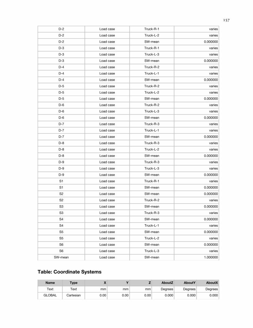
D-2 Load case Truck-R-1 varies
D-2 Load case Truck-L-2 varies
D-2 Load case SW-mean 0.000000
D-3 Load case Truck-R-1 varies
D-3 Load case Truck-L-3 varies
D-3 Load case SW-mean 0.000000
D-4 Load case Truck-R-2 varies
D-4 Load case Truck-L-1 varies
D-4 Load case SW-mean 0.000000
D-5 Load case Truck-R-2 varies
D-5 Load case Truck-L-2 varies
D-5 Load case SW-mean 0.000000
D-6 Load case Truck-R-2 varies
D-6 Load case Truck-L-3 varies
D-6 Load case SW-mean 0.000000
D-7 Load case Truck-R-3 varies
D-7 Load case Truck-L-1 varies
D-7 Load case SW-mean 0.000000
D-8 Load case Truck-R-3 varies
D-8 Load case Truck-L-2 varies
D-8 Load case SW-mean 0.000000
D-9 Load case Truck-R-3 varies
D-9 Load case Truck-L-3 varies
D-9 Load case SW-mean 0.000000
S1 Load case Truck-R-1 varies
S1 Load case SW-mean 0.000000
S2 Load case SW-mean 0.000000
S2 Load case Truck-R-2 varies
S3 Load case SW-mean 0.000000
S3 Load case Truck-R-3 varies
S4 Load case SW-mean 0.000000
S4 Load case Truck-L-1 varies
S5 Load case SW-mean 0.000000
S5 Load case Truck-L-2 varies
S6 Load case SW-mean 0.000000
S6 Load case Truck-L-3 varies
SW-mean Load case SW-mean 1.000000
Table: Coordinate Systems
Name Type X Y Z AboutZ AboutY AboutX
Text Text mm mm mm Degrees Degrees Degrees
GLOBAL Cartesian 0.00 0.00 0.00 0.000 0.000 0.000

Table: Frame Hinge Assigns 01 - Overview
Frame AssignType UserProp GenHinge RelDist AbsDist ActualDist OverWrites
Text Text Text Text Unitless mm mm Yes/No
6 User-defined FH2 6H1 0.9390 7699.80 7699.80 No
6 User-defined FH2 6H2 0.8780 7199.60 7199.60 No
6 User-defined FH2 6H3 0.8170 6699.40 6699.40 No
6 User-defined FH2 6H4 0.7560 6199.20 6199.20 No
6 User-defined FH-S 6H5 1.0000 8200.00 8200.00 No
7 User-defined FH2 7H1 0.0730 496.40 496.40 No
7 User-defined FH2 7H2 0.1470 999.60 999.60 No
7 User-defined FH2 7H3 0.2210 1502.80 1502.80 No
7 User-defined FH2 7H4 0.2940 1999.20 1999.20 No
7 User-defined FH-S 7H5 0.0000 0.00 0.00 No
9 User-defined FH1 9H1 0.1050 1102.50 1102.50 No
9 User-defined FH1 9H2 0.3050 3202.50 3202.50 No
9 User-defined FH1 9H3 0.5050 5302.50 5302.50 No
10 User-defined FH1 10H1 0.0960 998.40 998.40 No
10 User-defined FH1 10H2 0.2980 3099.20 3099.20 No
10 User-defined FH1 10H3 0.5000 5200.00 5200.00 No
10 User-defined FH1 10H4 0.7000 7280.00 7280.00 No
10 User-defined FH1 10H5 0.9000 9360.00 9360.00 No
11 User-defined FH1 11H1 0.1050 1102.50 1102.50 No
11 User-defined FH1 11H2 0.3050 3202.50 3202.50 No
11 User-defined FH1 11H3 0.5050 5302.50 5302.50 No
13 User-defined FH2 13H1 0.0730 496.40 496.40 No
13 User-defined FH2 13H2 0.1470 999.60 999.60 No
13 User-defined FH2 13H3 0.2210 1502.80 1502.80 No
13 User-defined FH2 13H4 0.2940 1999.20 1999.20 No
13 User-defined FH-S 13H5 0.0000 0.00 0.00 No
14 User-defined FH2 14H1 0.9390 7699.80 7699.80 No
14 User-defined FH2 14H2 0.8780 7199.60 7199.60 No
14 User-defined FH2 14H3 0.8170 6699.40 6699.40 No
14 User-defined FH2 14H4 0.7560 6199.20 6199.20 No
14 User-defined FH-S 14H5 1.0000 8200.00 8200.00 No
21 User-defined FH2 21H1 0.9390 7699.80 7699.80 No
21 User-defined FH2 21H2 0.8780 7199.60 7199.60 No
21 User-defined FH2 21H3 0.8170 6699.40 6699.40 No
21 User-defined FH2 21H4 0.7560 6199.20 6199.20 No
21 User-defined FH-S 21H5 1.0000 8200.00 8200.00 No
22 User-defined FH2 22H1 0.0730 496.40 496.40 No
22 User-defined FH2 22H2 0.1470 999.60 999.60 No
22 User-defined FH2 22H3 0.2210 1502.80 1502.80 No
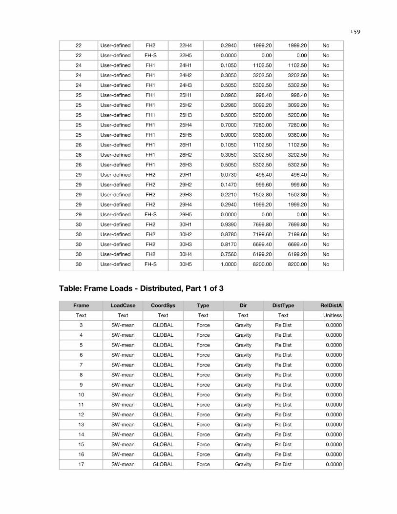
22 User-defined FH2 22H4 0.2940 1999.20 1999.20 No
22 User-defined FH-S 22H5 0.0000 0.00 0.00 No
24 User-defined FH1 24H1 0.1050 1102.50 1102.50 No
24 User-defined FH1 24H2 0.3050 3202.50 3202.50 No
24 User-defined FH1 24H3 0.5050 5302.50 5302.50 No
25 User-defined FH1 25H1 0.0960 998.40 998.40 No
25 User-defined FH1 25H2 0.2980 3099.20 3099.20 No
25 User-defined FH1 25H3 0.5000 5200.00 5200.00 No
25 User-defined FH1 25H4 0.7000 7280.00 7280.00 No
25 User-defined FH1 25H5 0.9000 9360.00 9360.00 No
26 User-defined FH1 26H1 0.1050 1102.50 1102.50 No
26 User-defined FH1 26H2 0.3050 3202.50 3202.50 No
26 User-defined FH1 26H3 0.5050 5302.50 5302.50 No
29 User-defined FH2 29H1 0.0730 496.40 496.40 No
29 User-defined FH2 29H2 0.1470 999.60 999.60 No
29 User-defined FH2 29H3 0.2210 1502.80 1502.80 No
29 User-defined FH2 29H4 0.2940 1999.20 1999.20 No
29 User-defined FH-S 29H5 0.0000 0.00 0.00 No
30 User-defined FH2 30H1 0.9390 7699.80 7699.80 No
30 User-defined FH2 30H2 0.8780 7199.60 7199.60 No
30 User-defined FH2 30H3 0.8170 6699.40 6699.40 No
30 User-defined FH2 30H4 0.7560 6199.20 6199.20 No
30 User-defined FH-S 30H5 1.0000 8200.00 8200.00 No
Table: Frame Loads - Distributed, Part 1 of 3
Frame LoadCase CoordSys Type Dir DistType RelDistA
Text Text Text Text Text Text Unitless
3 SW-mean GLOBAL Force Gravity RelDist 0.0000
4 SW-mean GLOBAL Force Gravity RelDist 0.0000
5 SW-mean GLOBAL Force Gravity RelDist 0.0000
6 SW-mean GLOBAL Force Gravity RelDist 0.0000
7 SW-mean GLOBAL Force Gravity RelDist 0.0000
8 SW-mean GLOBAL Force Gravity RelDist 0.0000
9 SW-mean GLOBAL Force Gravity RelDist 0.0000
10 SW-mean GLOBAL Force Gravity RelDist 0.0000
11 SW-mean GLOBAL Force Gravity RelDist 0.0000
12 SW-mean GLOBAL Force Gravity RelDist 0.0000
13 SW-mean GLOBAL Force Gravity RelDist 0.0000
14 SW-mean GLOBAL Force Gravity RelDist 0.0000
15 SW-mean GLOBAL Force Gravity RelDist 0.0000
16 SW-mean GLOBAL Force Gravity RelDist 0.0000
17 SW-mean GLOBAL Force Gravity RelDist 0.0000

18 SW-mean GLOBAL Force Gravity RelDist 0.0000
19 SW-mean GLOBAL Force Gravity RelDist 0.0000
20 SW-mean GLOBAL Force Gravity RelDist 0.0000
21 SW-mean GLOBAL Force Gravity RelDist 0.0000
22 SW-mean GLOBAL Force Gravity RelDist 0.0000
23 SW-mean GLOBAL Force Gravity RelDist 0.0000
24 SW-mean GLOBAL Force Gravity RelDist 0.0000
25 SW-mean GLOBAL Force Gravity RelDist 0.0000
26 SW-mean GLOBAL Force Gravity RelDist 0.0000
28 SW-mean GLOBAL Force Gravity RelDist 0.0000
29 SW-mean GLOBAL Force Gravity RelDist 0.0000
30 SW-mean GLOBAL Force Gravity RelDist 0.0000
31 SW-mean GLOBAL Force Gravity RelDist 0.0000
32 SW-mean GLOBAL Force Gravity RelDist 0.0000
33 SW-mean GLOBAL Force Gravity RelDist 0.0000
Table: Frame Loads - Distributed, Part 2 of 3
Frame LoadCase RelDistB AbsDistA AbsDistB FOverLA FOverLB
Text Text Unitless mm mm KN/mm KN/mm
3 SW-mean 1.0000 0.00 6800.00 0.07803 0.07803
4 SW-mean 1.0000 0.00 16000.00 0.07909 0.07909
5 SW-mean 1.0000 0.00 5000.00 0.08046 0.08046
6 SW-mean 1.0000 0.00 8200.00 0.08362 0.08362
7 SW-mean 1.0000 0.00 6800.00 0.08362 0.08362
8 SW-mean 1.0000 0.00 6000.00 0.07981 0.07981
9 SW-mean 1.0000 0.00 10500.00 0.07849 0.07849
10 SW-mean 1.0000 0.00 10400.00 0.07858 0.07858
11 SW-mean 1.0000 0.00 10500.00 0.07849 0.07849
12 SW-mean 1.0000 0.00 6000.00 0.07981 0.07981
13 SW-mean 1.0000 0.00 6800.00 0.08362 0.08362
14 SW-mean 1.0000 0.00 8200.00 0.08362 0.08362
15 SW-mean 1.0000 0.00 5000.00 0.08046 0.08046
16 SW-mean 1.0000 0.00 16000.00 0.07909 0.07909
17 SW-mean 1.0000 0.00 6800.00 0.07803 0.07803
18 SW-mean 1.0000 0.00 6800.00 0.07803 0.07803
19 SW-mean 1.0000 0.00 16000.00 0.07909 0.07909
20 SW-mean 1.0000 0.00 5000.00 0.08046 0.08046
21 SW-mean 1.0000 0.00 8200.00 0.08362 0.08362
22 SW-mean 1.0000 0.00 6800.00 0.08362 0.08362
23 SW-mean 1.0000 0.00 6000.00 0.07981 0.07981
24 SW-mean 1.0000 0.00 10500.00 0.07849 0.07849
25 SW-mean 1.0000 0.00 10400.00 0.07858 0.07858

26 SW-mean 1.0000 0.00 10500.00 0.07849 0.07849
28 SW-mean 1.0000 0.00 6000.00 0.07981 0.07981
29 SW-mean 1.0000 0.00 6800.00 0.08362 0.08362
30 SW-mean 1.0000 0.00 8200.00 0.08362 0.08362
31 SW-mean 1.0000 0.00 5000.00 0.08046 0.08046
32 SW-mean 1.0000 0.00 16000.00 0.07909 0.07909
33 SW-mean 1.0000 0.00 6800.00 0.07803 0.07803
Table: Frame Loads - Point, Part 1 of 2
Frame LoadCase CoordSys Type Dir DistType RelDist
Text Text Text Text Text Text Unitless
42 Truck-R-1 GLOBAL Moment Y RelDist 0.5920
42 Truck-R-1 GLOBAL Force Gravity RelDist 0.5920
42 Truck-R-1 GLOBAL Moment Y RelDist 0.8690
42 Truck-R-1 GLOBAL Force Gravity RelDist 0.8690
42 Truck-R-2 GLOBAL Force Gravity RelDist 0.5460
42 Truck-R-2 GLOBAL Force Gravity RelDist 0.8230
42 Truck-R-2 GLOBAL Moment Y RelDist 0.5460
42 Truck-R-2 GLOBAL Moment Y RelDist 0.8230
42 Truck-R-3 GLOBAL Force Gravity RelDist 0.5000
42 Truck-R-3 GLOBAL Force Gravity RelDist 0.7770
42 Truck-R-3 GLOBAL Moment Y RelDist 0.5000
42 Truck-R-3 GLOBAL Moment Y RelDist 0.7770
42 Truck-L-1 GLOBAL Force Gravity RelDist 0.0540
42 Truck-L-1 GLOBAL Force Gravity RelDist 0.3310
42 Truck-L-1 GLOBAL Moment Y RelDist 0.0540
42 Truck-L-1 GLOBAL Moment Y RelDist 0.3310
42 Truck-L-2 GLOBAL Force Gravity RelDist 0.0077
42 Truck-L-2 GLOBAL Force Gravity RelDist 0.2850
42 Truck-L-2 GLOBAL Moment Y RelDist 0.0077
42 Truck-L-2 GLOBAL Moment Y RelDist 0.2850
42 Truck-L-3 GLOBAL Force Gravity RelDist 0.2380
42 Truck-L-3 GLOBAL Moment Y RelDist 0.2380
43 test GLOBAL Force Gravity RelDist 0.0230
43 Truck-R-1 GLOBAL Force Gravity RelDist 0.5920
43 Truck-R-1 GLOBAL Force Gravity RelDist 0.8690
43 Truck-R-2 GLOBAL Force Gravity RelDist 0.5460
43 Truck-R-2 GLOBAL Force Gravity RelDist 0.8230
43 Truck-R-3 GLOBAL Force Gravity RelDist 0.5000
43 Truck-R-3 GLOBAL Force Gravity RelDist 0.7770
43 Truck-L-1 GLOBAL Force Gravity RelDist 0.0540
43 Truck-L-1 GLOBAL Force Gravity RelDist 0.3310
43 Truck-L-2 GLOBAL Force Gravity RelDist 0.0077

43 Truck-L-2 GLOBAL Force Gravity RelDist 0.2850
43 Truck-L-3 GLOBAL Force Gravity RelDist 0.2380
44 Truck-R-1 GLOBAL Moment Y RelDist 0.5920
44 Truck-R-1 GLOBAL Force Gravity RelDist 0.5920
44 Truck-R-1 GLOBAL Moment Y RelDist 0.8690
44 Truck-R-1 GLOBAL Force Gravity RelDist 0.8690
44 Truck-R-2 GLOBAL Force Gravity RelDist 0.5460
44 Truck-R-2 GLOBAL Force Gravity RelDist 0.8230
44 Truck-R-2 GLOBAL Moment Y RelDist 0.5460
44 Truck-R-2 GLOBAL Moment Y RelDist 0.8230
44 Truck-R-3 GLOBAL Force Gravity RelDist 0.5000
44 Truck-R-3 GLOBAL Force Gravity RelDist 0.7770
44 Truck-R-3 GLOBAL Moment Y RelDist 0.5000
44 Truck-R-3 GLOBAL Moment Y RelDist 0.7770
44 Truck-L-1 GLOBAL Force Gravity RelDist 0.0540
44 Truck-L-1 GLOBAL Force Gravity RelDist 0.3310
44 Truck-L-1 GLOBAL Moment Y RelDist 0.0540
44 Truck-L-1 GLOBAL Moment Y RelDist 0.3310
44 Truck-L-2 GLOBAL Force Gravity RelDist 0.0077
44 Truck-L-2 GLOBAL Force Gravity RelDist 0.2850
44 Truck-L-2 GLOBAL Moment Y RelDist 0.0077
44 Truck-L-2 GLOBAL Moment Y RelDist 0.2850
44 Truck-L-3 GLOBAL Force Gravity RelDist 0.2380
44 Truck-L-3 GLOBAL Moment Y RelDist 0.2380
66 Truck-L-3 GLOBAL Force Gravity RelDist 0.9020
66 Truck-L-3 GLOBAL Moment Y RelDist 0.9020
67 Truck-L-3 GLOBAL Force Gravity RelDist 0.9020
69 Truck-L-3 GLOBAL Force Gravity RelDist 0.9020
69 Truck-L-3 GLOBAL Moment Y RelDist 0.9020
110 Truck-L-3 GLOBAL Force Gravity RelDist 0.9020
110 Truck-L-3 GLOBAL Moment Y RelDist 0.9020
111 Truck-R-1 GLOBAL Moment Y RelDist 0.5920
111 Truck-R-1 GLOBAL Force Gravity RelDist 0.5920
111 Truck-R-1 GLOBAL Moment Y RelDist 0.8690
111 Truck-R-1 GLOBAL Force Gravity RelDist 0.8690
111 Truck-R-2 GLOBAL Force Gravity RelDist 0.5460
111 Truck-R-2 GLOBAL Force Gravity RelDist 0.8230
111 Truck-R-2 GLOBAL Moment Y RelDist 0.5460
111 Truck-R-2 GLOBAL Moment Y RelDist 0.8230
111 Truck-R-3 GLOBAL Force Gravity RelDist 0.5000
111 Truck-R-3 GLOBAL Force Gravity RelDist 0.7770
111 Truck-R-3 GLOBAL Moment Y RelDist 0.5000
111 Truck-R-3 GLOBAL Moment Y RelDist 0.7770
111 Truck-L-1 GLOBAL Force Gravity RelDist 0.0540

111 Truck-L-1 GLOBAL Force Gravity RelDist 0.3310
111 Truck-L-1 GLOBAL Moment Y RelDist 0.0540
111 Truck-L-1 GLOBAL Moment Y RelDist 0.3310
111 Truck-L-2 GLOBAL Force Gravity RelDist 0.0077
111 Truck-L-2 GLOBAL Force Gravity RelDist 0.2850
111 Truck-L-2 GLOBAL Moment Y RelDist 0.0077
111 Truck-L-2 GLOBAL Moment Y RelDist 0.2850
111 Truck-L-3 GLOBAL Force Gravity RelDist 0.2380
111 Truck-L-3 GLOBAL Moment Y RelDist 0.2380
Table: Frame Loads - Point, Part 2 of 2
Frame LoadCase AbsDist Force Moment GUID
Text Text mm KN KN-mm Text
42 Truck-d-1 1651.00 125.000
42 Truck-d-1 3347.50 125.000
42 Truck-d-1 5148.00 125.000
42 Truck-d-1 1651.00 -9375.00
42 Truck-d-1 3347.50 -9375.00
42 Truck-d-1 5148.00 -9375.00
42 Truck-R-1 1651.00 -9375.00
42 Truck-R-1 1651.00 125.000
42 Truck-R-2 149.50 125.000
42 Truck-R-2 1950.00 125.000
42 Truck-R-2 149.50 -9375.00
42 Truck-R-2 1950.00 -9375.00
42 Truck-R-3 448.50 125.000
42 Truck-R-3 2249.00 125.000
42 Truck-R-3 448.50 -9375.00
42 Truck-R-3 2249.00 -9375.00
42 Truck-L-1 3347.50 125.000
42 Truck-L-1 5148.00 125.000
42 Truck-L-1 3347.50 -9375.00
42 Truck-L-1 5148.00 -9375.00
42 Truck-L-2 3653.00 125.000
42 Truck-L-2 5447.00 125.000
42 Truck-L-2 3653.00 -9375.00
42 Truck-L-2 5447.00 -9375.00
42 Truck-L-3 3952.00 125.000
42 Truck-L-3 5752.50 125.000
42 Truck-L-3 3952.00 -9375.00
42 Truck-L-3 5752.50 -9375.00
43 Truck-d-1 1651.00 87.500
43 Truck-d-1 3347.50 87.500

43 Truck-d-1 5148.00 87.500
43 Truck-R-1 1651.00 87.500
43 Truck-R-2 149.50 87.500
43 Truck-R-2 1950.00 87.500
43 Truck-R-3 448.50 87.500
43 Truck-R-3 2249.00 87.500
43 Truck-L-1 3347.50 87.500
43 Truck-L-1 5148.00 87.500
43 Truck-L-2 3653.00 87.500
43 Truck-L-2 5447.00 87.500
43 Truck-L-3 3952.00 87.500
43 Truck-L-3 5752.50 87.500
44 Truck-d-1 1651.00 75.000
44 Truck-d-1 3347.50 75.000
44 Truck-d-1 5148.00 75.000
44 Truck-d-1 1651.00 -39375.00
44 Truck-d-1 3347.50 -39375.00
44 Truck-d-1 5148.00 -39375.00
44 Truck-R-1 1651.00 -39375.00
44 Truck-R-1 1651.00 75.000
44 Truck-R-2 149.50 75.000
44 Truck-R-2 1950.00 75.000
44 Truck-R-2 149.50 -39375.00
44 Truck-R-2 1950.00 -39375.00
44 Truck-R-3 448.50 75.000
44 Truck-R-3 2249.00 75.000
44 Truck-R-3 448.50 -39375.00
44 Truck-R-3 2249.00 -39375.00
44 Truck-L-1 3347.50 75.000
44 Truck-L-1 5148.00 75.000
44 Truck-L-1 3347.50 -39375.00
44 Truck-L-1 5148.00 -39375.00
44 Truck-L-2 3653.00 75.000
44 Truck-L-2 5447.00 75.000
44 Truck-L-2 3653.00 -39375.00
44 Truck-L-2 5447.00 -39375.00
44 Truck-L-3 3952.00 75.000
44 Truck-L-3 5752.50 75.000
44 Truck-L-3 3952.00 -39375.00
44 Truck-L-3 5752.50 -39375.00
66 Truck-d-1 2399.55 -42187.50
66 Truck-d-1 2399.55 62.500
66 Truck-d-1 2399.55 62.500
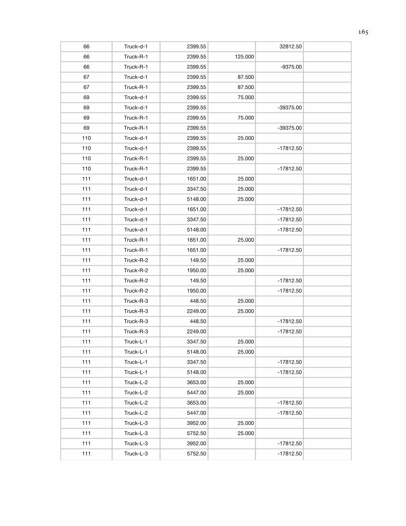
66 Truck-d-1 2399.55 32812.50
66 Truck-R-1 2399.55 125.000
66 Truck-R-1 2399.55 -9375.00
67 Truck-d-1 2399.55 87.500
67 Truck-R-1 2399.55 87.500
69 Truck-d-1 2399.55 75.000
69 Truck-d-1 2399.55 -39375.00
69 Truck-R-1 2399.55 75.000
69 Truck-R-1 2399.55 -39375.00
110 Truck-d-1 2399.55 25.000
110 Truck-d-1 2399.55 -17812.50
110 Truck-R-1 2399.55 25.000
110 Truck-R-1 2399.55 -17812.50
111 Truck-d-1 1651.00 25.000
111 Truck-d-1 3347.50 25.000
111 Truck-d-1 5148.00 25.000
111 Truck-d-1 1651.00 -17812.50
111 Truck-d-1 3347.50 -17812.50
111 Truck-d-1 5148.00 -17812.50
111 Truck-R-1 1651.00 25.000
111 Truck-R-1 1651.00 -17812.50
111 Truck-R-2 149.50 25.000
111 Truck-R-2 1950.00 25.000
111 Truck-R-2 149.50 -17812.50
111 Truck-R-2 1950.00 -17812.50
111 Truck-R-3 448.50 25.000
111 Truck-R-3 2249.00 25.000
111 Truck-R-3 448.50 -17812.50
111 Truck-R-3 2249.00 -17812.50
111 Truck-L-1 3347.50 25.000
111 Truck-L-1 5148.00 25.000
111 Truck-L-1 3347.50 -17812.50
111 Truck-L-1 5148.00 -17812.50
111 Truck-L-2 3653.00 25.000
111 Truck-L-2 5447.00 25.000
111 Truck-L-2 3653.00 -17812.50
111 Truck-L-2 5447.00 -17812.50
111 Truck-L-3 3952.00 25.000
111 Truck-L-3 5752.50 25.000
111 Truck-L-3 3952.00 -17812.50
111 Truck-L-3 5752.50 -17812.50

Table: Frame Section Assignments
Frame SectionType AutoSelect AnalSect DesignSect MatProp
Text Text Text Text Text Text
1 Rectangular N.A. T-SS-TYP T-SS-TYP Default
2 Rectangular N.A. T-SS-TYP T-SS-TYP Default
3 I/Wide Flange N.A. L1 L1 Default
4 I/Wide Flange N.A. L2 L2 Default
5 Nonprismatic N.A. VAR1 VAR1 Default
6 Nonprismatic N.A. VAR2 VAR2 Default
7 Nonprismatic N.A. VAR3 VAR3 Default
8 Nonprismatic N.A. VAR4 VAR4 Default
9 I/Wide Flange N.A. L9 L9 Default
10 I/Wide Flange N.A. L10 L10 Default
11 I/Wide Flange N.A. L9 L9 Default
12 Nonprismatic N.A. VAR4 VAR4 Default
13 Nonprismatic N.A. VAR3 VAR3 Default
14 Nonprismatic N.A. VAR2 VAR2 Default
15 Nonprismatic N.A. VAR1 VAR1 Default
16 I/Wide Flange N.A. L2 L2 Default
17 I/Wide Flange N.A. L1 L1 Default
18 I/Wide Flange N.A. L1 L1 Default
19 I/Wide Flange N.A. L2 L2 Default
20 Nonprismatic N.A. VAR1 VAR1 Default
21 Nonprismatic N.A. VAR2 VAR2 Default
22 Nonprismatic N.A. VAR3 VAR3 Default
23 Nonprismatic N.A. VAR4 VAR4 Default
24 I/Wide Flange N.A. L9 L9 Default
25 I/Wide Flange N.A. L10 L10 Default
26 I/Wide Flange N.A. L9 L9 Default
27 Rectangular N.A. T-SS-TYP T-SS-TYP Default
28 Nonprismatic N.A. VAR4 VAR4 Default
29 Nonprismatic N.A. VAR3 VAR3 Default
30 Nonprismatic N.A. VAR2 VAR2 Default
31 Nonprismatic N.A. VAR1 VAR1 Default
32 I/Wide Flange N.A. L2 L2 Default
33 I/Wide Flange N.A. L1 L1 Default
34 Rectangular N.A. T-S T-S Default
35 Rectangular N.A. T-SS-TYP T-SS-TYP Default
36 Rectangular N.A. T-SS-TYP T-SS-TYP Default
37 Rectangular N.A. T-SS-TYP T-SS-TYP Default
38 Rectangular N.A. T-SS-TYP T-SS-TYP Default
39 Rectangular N.A. T-PIER T-PIER Default
40 I/Wide Flange N.A. FSEC1 FSEC1 Default

41 Rectangular N.A. T-MS-TYP T-MS-TYP Default
42 Rectangular N.A. T-MS-TYP T-MS-TYP Default
43 Rectangular N.A. T-MS-TYP T-MS-TYP Default
44 Rectangular N.A. T-MS-TYP T-MS-TYP Default
45 Rectangular N.A. T-MS-TYP T-MS-TYP Default
46 Rectangular N.A. T-MS-TYP T-MS-TYP Default
47 Rectangular N.A. T-PIER T-PIER Default
48 Rectangular N.A. T-SS-TYP T-SS-TYP Default
49 Rectangular N.A. T-SS-TYP T-SS-TYP Default
50 Rectangular N.A. T-SS-TYP T-SS-TYP Default
51 Rectangular N.A. T-SS-TYP T-SS-TYP Default
52 Rectangular N.A. T-S T-S Default
53 Rectangular N.A. T-SS-TYP T-SS-TYP Default
54 Rectangular N.A. T-SS-TYP T-SS-TYP Default
55 Rectangular N.A. T-SS-TYP T-SS-TYP Default
56 Rectangular N.A. T-SS-TYP T-SS-TYP Default
57 Rectangular N.A. T-SS-TYP T-SS-TYP Default
58 Rectangular N.A. T-PIER T-PIER Default
59 Rectangular N.A. T-PIER T-PIER Default
61 Rectangular N.A. T-MS-TYP T-MS-TYP Default
62 Rectangular N.A. T-MS-TYP T-MS-TYP Default
63 Rectangular N.A. T-MS-TYP T-MS-TYP Default
64 Rectangular N.A. T-MS-TYP T-MS-TYP Default
65 Rectangular N.A. T-MS-TYP T-MS-TYP Default
66 Rectangular N.A. T-MS-TYP T-MS-TYP Default
67 Rectangular N.A. T-MS-TYP T-MS-TYP Default
68 Rectangular N.A. T-MS-TYP T-MS-TYP Default
69 Rectangular N.A. T-MS-TYP T-MS-TYP Default
70 Rectangular N.A. T-MS-TYP T-MS-TYP Default
71 Rectangular N.A. T-MS-TYP T-MS-TYP Default
72 Rectangular N.A. T-MS-TYP T-MS-TYP Default
74 Rectangular N.A. T-MS-TYP T-MS-TYP Default
75 Rectangular N.A. T-MS-TYP T-MS-TYP Default
76 Rectangular N.A. T-PIER T-PIER Default
77 Rectangular N.A. T-PIER T-PIER Default
78 Rectangular N.A. T-SS-TYP T-SS-TYP Default
79 Rectangular N.A. T-SS-TYP T-SS-TYP Default
80 Rectangular N.A. T-SS-TYP T-SS-TYP Default
81 Rectangular N.A. T-SS-TYP T-SS-TYP Default
82 Rectangular N.A. T-SS-TYP T-SS-TYP Default
83 Rectangular N.A. T-SS-TYP T-SS-TYP Default
84 Rectangular N.A. T-SS-TYP T-SS-TYP Default
85 Rectangular N.A. T-SS-TYP T-SS-TYP Default

86 Rectangular N.A. T-S T-S Default
87 Rectangular N.A. T-S T-S Default
88 Rectangular N.A. T-MS-TYP T-MS-TYP Default
96 Rectangular N.A. T-MS-TYP T-MS-TYP Default
97 Rectangular N.A. T-MS-TYP T-MS-TYP Default
98 Rectangular N.A. T-MS-TYP T-MS-TYP Default
99 Rectangular N.A. T-MS-TYP T-MS-TYP Default
100 Rectangular N.A. T-MS-TYP T-MS-TYP Default
101 Rectangular N.A. T-MS-TYP T-MS-TYP Default
102 Rectangular N.A. T-MS-TYP T-MS-TYP Default
103 Rectangular N.A. T-MS-TYP T-MS-TYP Default
104 Rectangular N.A. T-MS-TYP T-MS-TYP Default
105 Rectangular N.A. T-MS-TYP T-MS-TYP Default
106 Rectangular N.A. T-MS-TYP T-MS-TYP Default
107 Rectangular N.A. T-MS-TYP T-MS-TYP Default
108 Rectangular N.A. T-MS-TYP T-MS-TYP Default
109 Rectangular N.A. T-MS-TYP T-MS-TYP Default
110 Rectangular N.A. T-MS-TYP T-MS-TYP Default
111 Rectangular N.A. T-MS-TYP T-MS-TYP Default
112 Rectangular N.A. T-MS-TYP T-MS-TYP Default
113 Rectangular N.A. T-MS-TYP T-MS-TYP Default
114 Rectangular N.A. T-MS-TYP T-MS-TYP Default
115 Rectangular N.A. T-MS-TYP T-MS-TYP Default
116 Rectangular N.A. T-MS-TYP T-MS-TYP Default
117 Rectangular N.A. T-MS-TYP T-MS-TYP Default
118 Rectangular N.A. T-MS-TYP T-MS-TYP Default
119 Rectangular N.A. T-S T-S Default
120 Rectangular N.A. T-S T-S Default
Table: Frame Section Properties 01 - General, Part 1 of 6
SectionName Material Shape t3 t2 tf tw
Text Text Text mm mm mm mm
L1 Steel I/Wide Flange 1456.000 600.000 28.000 16.000
L10 Steel I/Wide Flange 1465.000 600.000 30.000 14.000
L2 Steel I/Wide Flange 1483.000 600.000 28.000 14.000
L3 Steel I/Wide Flange 1485.000 600.000 35.000 18.000
L4 Steel I/Wide Flange 1530.000 600.000 35.000 18.000
L5 Steel I/Wide Flange 1575.000 60.000 600.000 20.000
L6 Steel I/Wide Flange 2130.000 600.000 60.000 20.000
L7 Steel I/Wide Flange 1515.000 600.000 30.000 20.000
L8 Steel I/Wide Flange 1470.000 600.000 30.000 20.000
L9 Steel I/Wide Flange 1463.000 600.000 28.000 14.000

T-MS-TYP CONC Rectangular 225.000 3562.500
T-PIER CONC Rectangular 225.000 5381.250
T-S CONC Rectangular 225.000 3600.000
T-SS-TYP CONC Rectangular 225.000 7200.000
VAR1 Nonprismatic
VAR2 Nonprismatic
VAR3 Nonprismatic
VAR4 Nonprismatic
Table: Frame Section Properties 01 - General, Part 2 of 6
SectionName t2b tfb Area TorsConst I33 I22 AS2
Text mm mm mm2 mm4 mm4 mm4 mm2
L1 600.000 28.000 56000.00 10420348.59 2.079E+10 1008477867 23296.00
L10 725.000 35.000 62975.00 16548693.06 2.502E+10 1651797998 20510.00
L2 600.000 55.000 69400.00 36887156.96 2.716E+10 1494320133 20762.00
L3 800.000 50.000 86200.00 42980257.12 3.371E+10 2764013733 26730.00
L4 800.000 50.000 87010.00 43067737.12 3.602E+10 2764035603 27540.00
L5 800.000 70.000 110100.00 129282700.0 3.603E+10 2998070000 31500.00
L6 800.000 70.000 132000.00 132202700.0 1.082E+11 4068000000 42600.00
L7 800.000 40.000 78900.00 25578700.00 3.107E+10 2247630000 30300.00
L8 800.000 40.000 78000.00 25458700.00 2.904E+10 2247600000 29400.00
L9 725.000 35.000 61775.00 15580115.30 2.421E+10 1615797998 20482.00
T-MS-TYP 801562.50 1.299E+10 3381591797 8.477E+11 667968.75
T-PIER 1210781.25 1.989E+10 5107983398 2.922E+12 1008984.38
T-S 810000.00 1.313E+10 3417187500 8.748E+11 675000.00
T-SS-TYP 1620000.00 2.680E+10 6834375000 6.998E+12 1350000.00
VAR1
VAR2
VAR3
VAR4
Table: Frame Section Properties 01 - General, Part 3 of 6SectionName AS3 S33 S22 Z33 Z22 R33 R22
Text mm2 mm3 mm3 mm3 mm3 mm mm
L1 28000.00 28557702.56 3361592.89 31830400.00 5129600.00 609.303 134.196
L10 36145.83 30707068.60 4556684.13 36965301.34 7367818.75 630.296 161.955
L2 41500.00 30143113.80 4981067.11 38176271.43 7538600.00 625.602 146.738
L3 50833.33 37596892.75 6910034.33 47873611.11 11263400.00 625.358 179.067
L4 50833.33 39040287.58 6910089.01 49822223.61 11267045.00 643.375 178.233
L5 76666.67 34172564.89 7495175.00 53529121.88 11830500.00 572.070 165.016
L6 76666.67 88857970.15 10170000.00 110040000.0 16800000.00 905.560 175.551
L7 41666.67 35095325.06 5619075.00 45025125.00 9244500.00 627.557 168.781

L8 41666.67 33756750.11 5619000.00 43260000.00 9240000.00 610.210 169.751
L9 35145.83 29217688.05 4457373.79 35748715.63 7187818.75 626.002 161.729
T-MS-TYP 667968.75 30058593.75 475927734. 45087890.63 713891602. 64.952 1028.405
T-PIER 1008984.38 45404296.88 1085919434 68106445.31 1628879150 64.952 1553.433
T-S 675000.00 30375000.00 486000000. 45562500.00 729000000. 64.952 1039.230
T-SS-TYP 1350000.00 60750000.00 1944000000 91125000.00 2916000000 64.952 2078.461
VAR1
VAR2
VAR3
VAR4
Table: Frame Section Properties 01 - General, Part 5 of 6
SectionName A2Mod A3Mod JMod I2Mod I3Mod MMod WMod
Text Unitless Unitless Unitless Unitless Unitless Unitless Unitless
L1 1.000000 1.000000 331.000000 1.000000 2.519000 1.000000 1.000000
L10 1.000000 1.000000 208.000000 1.000000 2.670000 1.000000 1.000000
L2 1.000000 1.000000 92.000000 1.000000 2.968000 1.000000 1.000000
L3 1.000000 1.000000 80.000000 1.000000 2.832000 1.000000 1.000000
L4 1.000000 1.000000 80.000000 1.000000 2.815000 1.000000 1.000000
L5 1.000000 1.000000 26.000000 1.000000 2.417000 1.000000 1.000000
L6 1.000000 1.000000 26.000000 1.000000 2.297000 1.000000 1.000000
L7 1.000000 1.000000 135.000000 1.000000 2.829000 1.000000 1.000000
L8 1.000000 1.000000 136.000000 1.000000 2.846000 1.000000 1.000000
L9 1.000000 1.000000 221.000000 1.000000 2.752000 1.000000 1.000000
T-MS-TYP 1.000000 1.000000 1.000000 1.000000 1.000000 1.000000 1.000000
T-PIER 1.000000 1.000000 1.000000 1.000000 1.000000 1.000000 1.000000
T-S 1.000000 1.000000 1.000000 1.000000 1.000000 1.000000 1.000000
T-SS-TYP 1.000000 1.000000 1.000000 1.000000 1.000000 1.000000 1.000000
VAR1
VAR2
VAR3
VAR4
Table: Frame Section Properties 05 - Nonprismatic, Part 1 of 2
SectionName NumSegments SegmentNum StartSect EndSect LengthType AbsLength
Text Unitless Unitless Text Text Text mm
VAR1 1 1 L3 L4 Variable
VAR2 1 1 L5 L6 Variable
VAR3 1 1 L6 L5 Variable
VAR4 1 1 L7 L8 Variable
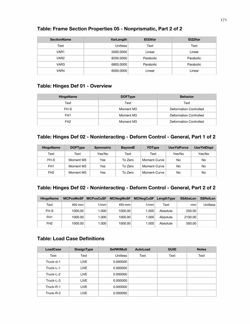
Table: Frame Section Properties 05 - Nonprismatic, Part 2 of 2
SectionName VarLength EI33Var EI22Var
Text Unitless Text Text
VAR1 5000.0000 Linear Linear
VAR2 8200.0000 Parabolic Parabolic
VAR3 6800.0000 Parabolic Parabolic
VAR4 6000.0000 Linear Linear
Table: Hinges Def 01 - Overview
HingeName DOFType Behavior
Text Text Text
FH-S Moment M3 Deformation Controlled
FH1 Moment M3 Deformation Controlled
FH2 Moment M3 Deformation Controlled
Table: Hinges Def 02 - Noninteracting - Deform Control - General, Part 1 of 2
HingeName DOFType Symmetric BeyondE FDType UseYldForce UseYldDispl
Text Text Yes/No Text Text Yes/No Yes/No
FH-S Moment M3 Yes To Zero Moment-Curve No No
FH1 Moment M3 Yes To Zero Moment-Curve No No
FH2 Moment M3 Yes To Zero Moment-Curve No No
Table: Hinges Def 02 - Noninteracting - Deform Control - General, Part 2 of 2
HingeName MCPosMoSF MCPosCuSF MCNegMoSF MCNegCuSF LengthType SSAbsLen SSRelLen
Text KN-mm 1/mm KN-mm 1/mm Text mm Unitless
FH-S 1000.00 1.000 1000.00 1.000 Absolute 250.00
FH1 1000.00 1.000 1000.00 1.000 Absolute 2100.00
FH2 1000.00 1.000 1000.00 1.000 Absolute 500.00
Table: Load Case Definitions
LoadCase DesignType SelfWtMult AutoLoad GUID Notes
Text Text Unitless Text Text Text
Truck-d-1 LIVE 0.000000
Truck-L-1 LIVE 0.000000
Truck-L-2 LIVE 0.000000
Truck-L-3 LIVE 0.000000
Truck-R-1 LIVE 0.000000
Truck-R-2 LIVE 0.000000

Truck-R-3 LIVE 0.000000
SW-mean LIVE 0.000000

Appendix E
The Double-T Girder Bridge - Drawings
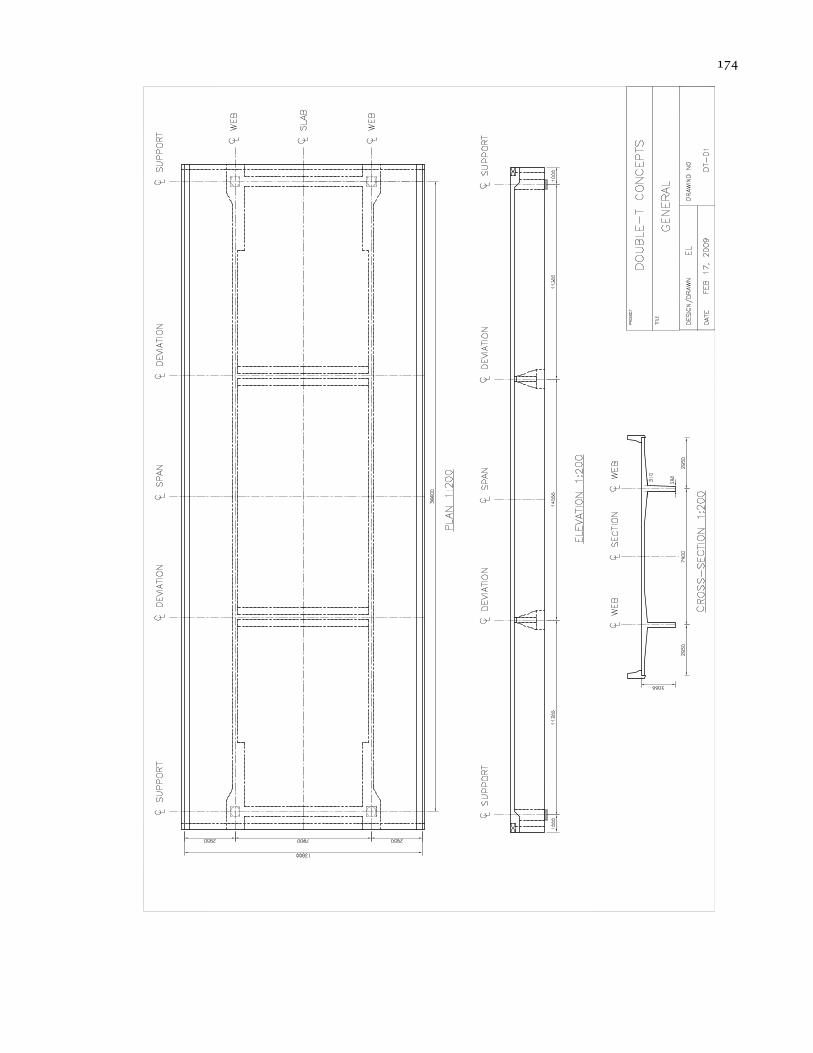
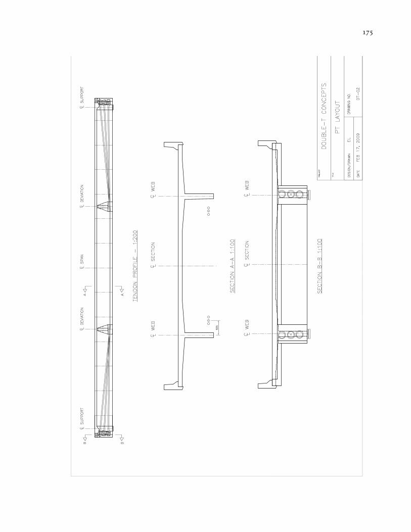
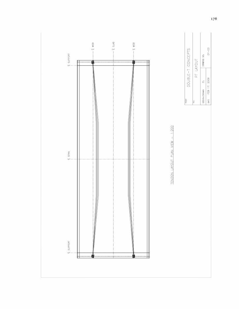

Appendix F
Excel Spreadsheet and Macros for Nonlinear Analysis of the Double-T Girder Bridge

SubMomCurv()''Macro1Macro'Macrorecorded2/4/2010byN'
Cells(82,2).Value=Cells(7,2).Value
M=0ecp=0etop=0ebottom=0curvature=0Fori=0To14Mom=Cells(11+i,6).Valueresult=0
Cells(85,4).Value=0.45*10^‐3'startwith0.02Cells(143,4).Value=‐0.6*10^‐4ForY=0To150Ifresult=0ThenSolverOkSetCell:="$H$145",MaxMinVal:=3,ValueOf:="0",
ByChange:="$D$143"SolverOkSetCell:="$H$145",MaxMinVal:=3,ValueOf:="0", ByChange:="$D$143"SolverDeleteCellRef:="$D$143",Relation:=3,FormulaText:="‐3.5*10^‐3"SolverAddCellRef:="$D$143",Relation:=3,FormulaText:="‐3.5*10^‐3"SolverOkSetCell:="$H$145",MaxMinVal:=3,ValueOf:="0", ByChange:="$D$143"SolverSolveuserFinish:=TrueIfCells(145,8).Value<100ThenCells(166+Y,8).Value=1Cells(166+Y,9).Value=Cells(144,9).ValueElseCells(166+Y,8).Value=0Cells(143,4).Value=0.0003EndIfCells(157,2).Value=‐Cells(11+i,2)*1000+353

Mo=Metopo=etopebottomo=ebottomecpo=ecpcurvatureo=curvatureM=Cells(144,9).Valueetop=Cells(85,4).Valueebottom=Cells(143,4).Valueecp=Cells(159,2).Valuecurvature=Cells(161,2).ValueIfM>MomThen
result=1Cells(11+i,8)=1/(M‐Mo)*(ecp‐ecpo)*(Mom‐Mo)+ecpoCells(11+i,9)=1/(M‐Mo)*(etop‐etopo)*(Mom‐Mo)+etopoCells(11+i,10)=1/(M‐Mo)*(ebottom‐ebottomo)*(Mom‐Mo)+
ebottomoCells(11+i,14)=1/(M‐Mo)*(curvature‐curvatureo)*(Mom‐Mo)
+curvatureoEndIfCells(166+i,8).Value=MCells(85,4).Value=Cells(85,4).Value‐0.02*10^‐3EndIfNextNext
Cells(82,2).Value=Cells(7,2).Value
EndSub

Subsecondary()''secondaryMacro'Macrorecorded3/9/2010byN
Fori=1To15ratio=Cells(38+i,1).Value/36.6Cells(4,15).Value=ratioCells(38+i,2).Value=Cells(27,16).ValueNextratio=11.3/36.6Cells(4,15).Value=ratioCells(34,2).Value=Cells(27,16).Value
'Solve:
Cells(82,2).Value=Cells(7,2).ValueCount=0
M=0ecp=0etop=0ebottom=0curvature=0Fori=0To14Mom=Cells(39+i,8).Valueresult=0
Cells(85,4).Value=0.45*10^‐3'startwith0.02Cells(143,4).Value=‐0.6*10^‐4
ForY=0To150Ifresult=0ThenSolverOkSetCell:="$H$145",MaxMinVal:=3,ValueOf:="0",
ByChange:="$D$143"SolverOkSetCell:="$H$145",MaxMinVal:=3,ValueOf:="0",
ByChange:="$D$143"SolverDeleteCellRef:="$D$143",Relation:=3,FormulaText:="‐3.5*10^‐3"SolverAddCellRef:="$D$143",Relation:=3,FormulaText:="‐3.5*10^‐3"SolverOkSetCell:="$H$145",MaxMinVal:=3,ValueOf:="0",
ByChange:="$D$143"SolverSolveuserFinish:=True

IfCells(145,8).Value<100ThenCells(166+Y,4).Value=1ElseCells(166+Y,4).Value=0Cells(143,4).Value=0.0003EndIfCells(157,2).Value=‐Cells(39+i,4)*1000+353‐Cells(39+i,2)Mo=Metopo=etopebottomo=ebottomecpo=ecpcurvatureo=curvatureM=Cells(144,9).Valueetop=Cells(85,4).Valueebottom=Cells(143,4).Valueecp=Cells(159,2).Valuecurvature=Cells(161,2).ValueIfM>MomThen
result=1Cells(39+i,10)=1/(M‐Mo)*(ecp‐ecpo)*(Mom‐Mo)+ecpoCells(39+i,11)=1/(M‐Mo)*(etop‐etopo)*(Mom‐Mo)+etopoCells(39+i,12)=1/(M‐Mo)*(ebottom‐ebottomo)*(Mom‐Mo)+
ebottomoCells(39+i,16)=1/(M‐Mo)*(curvature‐curvatureo)*(Mom‐Mo)
+curvatureoEndIfCells(166+i,8).Value=MCells(85,4).Value=Cells(85,4).Value‐0.02*10^‐3EndIfNextNext
Cells(82,2).Value=Cells(7,2).Value
EndSub
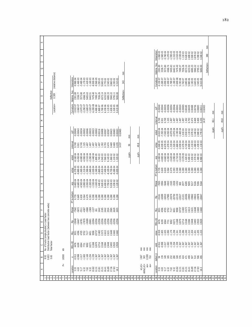
1 2 3 4 5 6 7 8 9 10
11
12
13
14
15
16
17
18
19
20
21
22
23
24
25
26
27
28
29
30
31
32
33
34
35
36
37
38
39
40
41
42
43
44
45
46
47
48
49
50
51
52
53
54
55
56
57
58
59
60
61
AB
CD
EF
GH
IJ
KL
MN
OP
QR
S
8.9
2N
o. o
f tr
ucks
(si
ngle
,dou
ble)
x L
oad
fact
or
0.6
53
Dis
trib
utio
n lo
ad fac
tor
(bet
wee
n tw
o co
ncre
te w
ebs)
5.8
2To
tal f
acto
r
Loca
tion
=0.3
09
(rel
ativ
e di
stan
ce)
P=16500
kN
Loca
tion
eM
DL+
SI
MLL
Mp
Mto
tal
PT t
o bo
ttom
ecp
ecto
pec
bot
Lint
erva
l !
LPCur
vatu
reH
elpi
ng Sys
.In
tegr
atio
n
3.3
3-0
.912
4476
3031
-15048
-7542
0.7
35
-5.4
0E-
04
-6.3
7E-
05
-8.1
6E-
04
0.7
49
-0.0
0040
-3.9
1E-
07
2301.8
9-9
.98E-
04
4.8
3-0
.998
6199
4396
-16467
-5872
0.6
49
-4.6
8E-
04
-9.8
8E-
05
-6.4
5E-
04
0.9
21
-0.0
0043
-3.0
6E-
07
3338.7
7-1
.46E-
03
5.1
7-1
.017
6564
4705
-16781
-5511
0.6
30
-4.5
0E-
04
-1.0
6E-
04
-6.0
8E-
04
0.7
49
-0.0
0034
-2.8
7E-
07
3573.8
0-3
.48E-
04
6.3
2-1
.083
7731
5752
-17870
-4387
0.5
64
-3.8
9E-
04
-1.3
1E-
04
-4.9
0E-
04
1.3
25
-0.0
0052
-2.2
9E-
07
4368.7
4-1
.17E-
03
7.8
2-1
.169
9092
7117
-19289
-3080
0.4
79
-3.0
5E-
04
-1.5
9E-
04
-3.5
1E-
04
1.4
97
-0.0
0046
-1.6
0E-
07
5405.6
3-1
.42E-
03
9.3
2-1
.254
10271
8451
-20691
-1969
0.3
93
-2.2
0E-
04
-1.8
4E-
04
-2.2
9E-
04
1.4
97
-0.0
0033
-1.0
2E-
07
6442.5
1-1
.16E-
03
10.8
2-1
.339
11268
9598
-22094
-1227
0.3
08
-1.5
3E-
04
-2.0
2E-
04
-1.4
4E-
04
1.4
97
-0.0
0023
-6.2
0E-
08
7479.4
0-8
.50E-
04
12.3
1-1
.367
12079
10737
-22556
261
0.2
80
-1.6
5E-
05
-2.3
4E-
04
1.8
9E-
05
1.4
97
-0.0
0002
4.4
8E-
08
7499.3
7-9
.56E-
05
13.8
1-1
.367
12714
11483
-22556
1642
0.2
80
1.4
4E-
03
-3.8
6E-
04
1.7
4E-
03
1.4
97
0.0
0216
1.8
6E-
07
7036.2
61.2
5E-
03
15.3
1-1
.367
13168
11573
-22556
2185
0.2
80
3.8
2E-
03
-5.8
1E-
04
4.5
4E-
03
1.3
02
0.0
0498
1.7
6E-
06
6573.1
49.8
4E-
03
16.4
1-1
.367
13384
11613
-22556
2442
0.2
80
6.4
0E-
03
-7.4
0E-
04
7.5
6E-
03
0.7
93
0.0
0507
6.1
5E-
06
6233.5
22.7
7E-
02
16.8
9-1
.367
13448
11631
-22556
2524
0.2
80
7.7
5E-
03
-8.1
0E-
04
9.1
4E-
03
0.4
74
0.0
0367
1.1
1E-
05
6085.3
32.5
4E-
02
17.3
6-1
.367
13493
11648
-22556
2585
0.2
80
9.0
3E-
03
-8.7
3E-
04
1.0
6E-
02
0.4
69
0.0
0423
1.6
3E-
05
5940.2
23.8
6E-
02
17.8
3-1
.367
13520
11665
-22556
2629
0.2
80
1.0
3E-
02
-9.2
8E-
04
1.2
1E-
02
0.4
69
0.0
0483
1.5
2E-
05
5795.1
14.3
3E-
02
18.3
-1.3
67
13529
11682
-22556
2655
0.2
80
1.1
2E-
02
-9.6
5E-
04
1.3
2E-
02
0.2
35
0.0
0263
9.4
1E-
06
5650.0
03.3
1E-
02
14.9
70.0
2485
Def
lect
ion=
343
mm
!Lp
d=50
mm
!Lp
f=49.8
mm
e(i,d)
=1367
mm
delta(
i,d)
=343
mm
ao=
11300
mm
es=
722
mm
Loca
tion
delta(
i,j)
eold
enew
MD
L+SI
MLL
Mp
Mto
tal
PT t
o bo
ttom
ecp
ecto
pec
bot
Lint
erva
l !
LPCur
vatu
reH
elpi
ng Sys
.In
tegr
atio
n
3.3
394
-0.9
12
-0.9
19
4476
3031
-15161
-7655
0.7
35
-5.4
0E-
04
-5.0
4E-
05
-8.8
1E-
04
0.7
49
-0.0
0040
-4.1
5E-
07
2301.8
9-1
.06E-
03
4.8
3139
-0.9
98
-1.0
05
6199
4396
-16589
-5994
0.6
49
-4.8
0E-
04
-8.0
3E-
05
-7.3
5E-
04
0.9
21
-0.0
0044
-3.2
8E-
07
3338.7
7-1
.56E-
03
5.1
7149
-1.0
17
-1.0
25
6564
4705
-16910
-5640
0.6
30
-4.6
6E-
04
-8.6
7E-
05
-7.0
4E-
04
0.7
49
-0.0
0035
-3.0
9E-
07
3573.8
0-3
.74E-
04
6.3
2185
-1.0
83
-1.0
90
7731
5752
-17985
-4503
0.5
64
-4.2
0E-
04
-1.0
7E-
04
-6.0
5E-
04
1.3
25
-0.0
0056
-2.4
9E-
07
4368.7
4-1
.27E-
03
7.8
2232
-1.1
69
-1.1
74
9092
7117
-19374
-3165
0.4
79
-3.6
2E-
04
-1.3
1E-
04
-4.8
7E-
04
1.4
97
-0.0
0054
-1.7
8E-
07
5405.6
3-1
.55E-
03
9.3
2280
-1.2
54
-1.2
58
10271
8451
-20750
-2028
0.3
93
-3.0
9E-
04
-1.5
2E-
04
-3.8
7E-
04
1.4
97
-0.0
0046
-1.1
8E-
07
6442.5
1-1
.31E-
03
10.8
2328
-1.3
39
-1.3
41
11268
9598
-22119
-1252
0.3
08
-2.7
1E-
04
-1.6
6E-
04
-3.1
9E-
04
1.4
97
-0.0
0041
-7.6
9E-
08
7479.4
0-1
.01E-
03
12.3
1376
-1.3
67
-1.3
34
12079
10737
-22017
800
0.2
80
-1.6
1E-
04
-2.0
3E-
04
-1.4
0E-
04
1.4
97
-0.0
0024
3.1
5E-
08
7499.3
7-2
.53E-
04
13.8
1424
-1.3
67
-1.2
86
12714
11483
-21221
2977
0.2
80
-3.5
7E-
05
-2.4
7E-
04
1.0
1E-
04
1.4
97
-0.0
0005
1.7
4E-
07
7036.2
61.1
1E-
03
15.3
1471
-1.3
67
-1.2
40
13168
11573
-20456
4285
0.2
80
1.4
2E-
03
-4.7
2E-
04
2.9
1E-
03
1.3
02
0.0
0185
1.6
9E-
06
6573.1
49.4
2E-
03
16.4
1499
-1.3
67
-1.2
12
13384
11613
-19993
5005
0.2
80
5.4
9E-
03
-8.9
0E-
04
1.1
1E-
02
0.7
93
0.0
0435
5.9
8E-
06
6233.5
22.6
9E-
02
16.8
9507
-1.3
67
-1.2
04
13448
11631
-19862
5217
0.2
80
1.0
3E-
02
-1.2
1E-
03
2.0
7E-
02
0.4
74
0.0
0488
1.1
0E-
05
6085.3
32.5
0E-
02
17.3
6510
-1.3
67
-1.2
01
13493
11648
-19815
5326
0.2
80
1.5
7E-
02
-1.4
8E-
03
3.1
4E-
02
0.4
69
0.0
0736
1.6
4E-
05
5940.2
23.8
7E-
02
17.8
3506
-1.3
67
-1.2
05
13520
11665
-19878
5306
0.2
80
1.4
8E-
02
-1.4
3E-
03
2.9
4E-
02
0.4
69
0.0
0693
1.5
4E-
05
5795.1
14.3
9E-
02
18.3
495
-1.3
67
-1.2
15
13529
11682
-20047
5164
0.2
80
8.9
8E-
03
-1.1
1E-
03
1.7
7E-
02
0.2
35
0.0
0211
9.4
1E-
06
5650.0
03.3
4E-
02
14.9
70.0
2403
Def
lect
ion=
340
mm
!Lp
d=48.1
mm
!Lp
f=49.8
mm
Def
lect
ion

Appendix G
e Double-T Girder Bridge - SAP2000 Input File
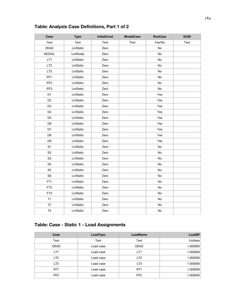
Table: Analysis Case Definitions, Part 1 of 2
Case Type InitialCond ModalCase RunCase GUID
Text Text Text Text Yes/No Text
DEAD LinStatic Zero No
MODAL LinModal Zero No
LT1 LinStatic Zero No
LT2 LinStatic Zero No
LT3 LinStatic Zero No
RT1 LinStatic Zero No
RT2 LinStatic Zero No
RT3 LinStatic Zero No
D1 LinStatic Zero Yes
D2 LinStatic Zero Yes
D3 LinStatic Zero Yes
D4 LinStatic Zero Yes
D5 LinStatic Zero Yes
D6 LinStatic Zero Yes
D7 LinStatic Zero Yes
D8 LinStatic Zero Yes
D9 LinStatic Zero Yes
S1 LinStatic Zero No
S2 LinStatic Zero No
S3 LinStatic Zero No
S4 LinStatic Zero No
S5 LinStatic Zero No
S6 LinStatic Zero No
FT1 LinStatic Zero No
FT2 LinStatic Zero No
FT3 LinStatic Zero No
T1 LinStatic Zero No
T2 LinStatic Zero No
T3 LinStatic Zero No
Table: Case - Static 1 - Load Assignments
Case LoadType LoadName LoadSF
Text Text Text Unitless
DEAD Load case DEAD 1.000000
LT1 Load case LT1 1.000000
LT2 Load case LT2 1.000000
LT3 Load case LT3 1.000000
RT1 Load case RT1 1.000000
RT2 Load case RT2 1.000000
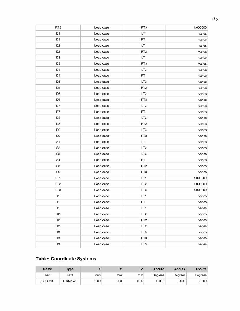
RT3 Load case RT3 1.000000
D1 Load case LT1 varies
D1 Load case RT1 varies
D2 Load case LT1 varies
D2 Load case RT2 Varies
D3 Load case LT1 varies
D3 Load case RT3 Varies
D4 Load case LT2 varies
D4 Load case RT1 varies
D5 Load case LT2 varies
D5 Load case RT2 varies
D6 Load case LT2 varies
D6 Load case RT3 varies
D7 Load case LT3 varies
D7 Load case RT1 varies
D8 Load case LT3 varies
D8 Load case RT2 varies
D9 Load case LT3 varies
D9 Load case RT3 varies
S1 Load case LT1 varies
S2 Load case LT2 varies
S3 Load case LT3 varies
S4 Load case RT1 varies
S5 Load case RT2 varies
S6 Load case RT3 varies
FT1 Load case FT1 1.000000
FT2 Load case FT2 1.000000
FT3 Load case FT3 1.000000
T1 Load case FT1 varies
T1 Load case RT1 varies
T1 Load case LT1 varies
T2 Load case LT2 varies
T2 Load case RT2 varies
T2 Load case FT2 varies
T3 Load case LT3 varies
T3 Load case RT3 varies
T3 Load case FT3 varies
Table: Coordinate Systems
Name Type X Y Z AboutZ AboutY AboutX
Text Text mm mm mm Degrees Degrees Degrees
GLOBAL Cartesian 0.00 0.00 0.00 0.000 0.000 0.000

Table: Frame Loads - Point, Part 1 of 2
Frame LoadCase CoordSys Type Dir DistType RelDist
Text Text Text Text Text Text Unitless
43 LT1 GLOBAL Force Gravity RelDist 0.5650
43 LT2 GLOBAL Force Gravity RelDist 0.7180
43 LT3 GLOBAL Force Gravity RelDist 0.8700
43 LT1 GLOBAL Moment Y RelDist 0.5650
43 LT2 GLOBAL Moment Y RelDist 0.7180
43 LT3 GLOBAL Moment Y RelDist 0.8700
45 FT1 GLOBAL Force Gravity RelDist 0.1320
45 FT1 GLOBAL Moment Y RelDist 0.1320
45 FT2 GLOBAL Force Gravity RelDist 0.2840
45 FT3 GLOBAL Force Gravity RelDist 0.4360
45 FT3 GLOBAL Moment Y RelDist 0.4360
45 FT2 GLOBAL Moment Y RelDist 0.2840
73 LT1 GLOBAL Force Gravity RelDist 0.5650
73 LT2 GLOBAL Force Gravity RelDist 0.7180
73 LT3 GLOBAL Force Gravity RelDist 0.8700
73 LT1 GLOBAL Moment Y RelDist 0.5650
73 LT2 GLOBAL Moment Y RelDist 0.7180
73 LT3 GLOBAL Moment Y RelDist 0.8700
75 FT1 GLOBAL Force Gravity RelDist 0.1320
75 FT1 GLOBAL Moment Y RelDist 0.1320
75 FT2 GLOBAL Force Gravity RelDist 0.2840
75 FT3 GLOBAL Force Gravity RelDist 0.4360
75 FT3 GLOBAL Moment Y RelDist 0.4360
75 FT2 GLOBAL Moment Y RelDist 0.2840
85 LT1 GLOBAL Force Gravity RelDist 0.5650
85 LT2 GLOBAL Force Gravity RelDist 0.7180
85 LT3 GLOBAL Force Gravity RelDist 0.8700
85 LT1 GLOBAL Moment Y RelDist 0.5650
85 LT2 GLOBAL Moment Y RelDist 0.7180
85 LT3 GLOBAL Moment Y RelDist 0.8700
87 FT1 GLOBAL Force Gravity RelDist 0.1320
87 FT1 GLOBAL Moment Y RelDist 0.1320
87 FT2 GLOBAL Force Gravity RelDist 0.2840
87 FT3 GLOBAL Force Gravity RelDist 0.4360
87 FT3 GLOBAL Moment Y RelDist 0.4360
87 FT2 GLOBAL Moment Y RelDist 0.2840
88 LT1 GLOBAL Force Gravity RelDist 0.5650
88 LT2 GLOBAL Force Gravity RelDist 0.7180
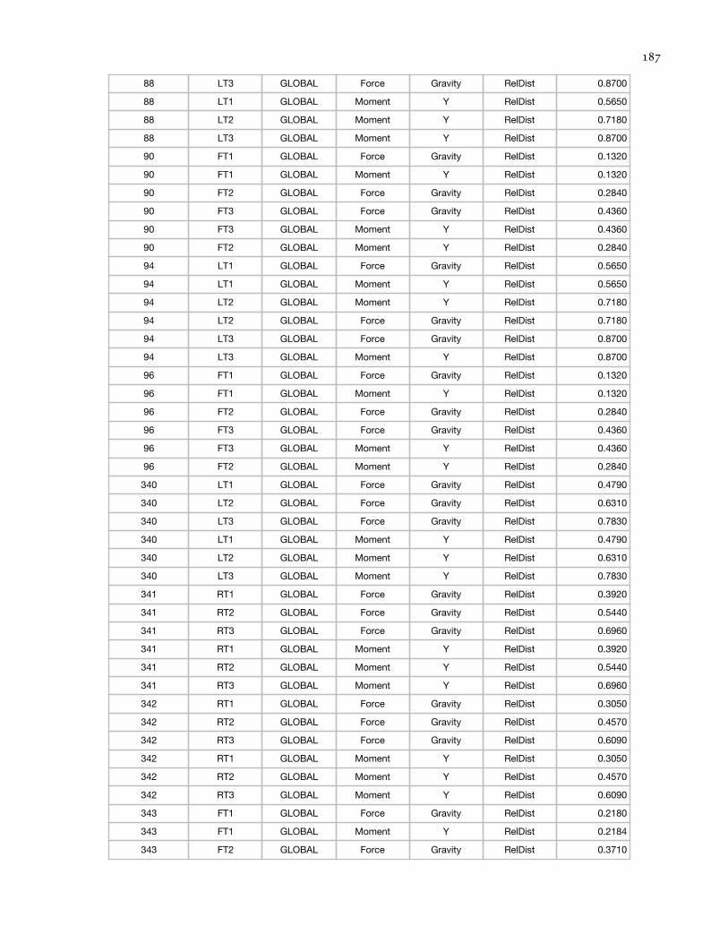
88 LT3 GLOBAL Force Gravity RelDist 0.8700
88 LT1 GLOBAL Moment Y RelDist 0.5650
88 LT2 GLOBAL Moment Y RelDist 0.7180
88 LT3 GLOBAL Moment Y RelDist 0.8700
90 FT1 GLOBAL Force Gravity RelDist 0.1320
90 FT1 GLOBAL Moment Y RelDist 0.1320
90 FT2 GLOBAL Force Gravity RelDist 0.2840
90 FT3 GLOBAL Force Gravity RelDist 0.4360
90 FT3 GLOBAL Moment Y RelDist 0.4360
90 FT2 GLOBAL Moment Y RelDist 0.2840
94 LT1 GLOBAL Force Gravity RelDist 0.5650
94 LT1 GLOBAL Moment Y RelDist 0.5650
94 LT2 GLOBAL Moment Y RelDist 0.7180
94 LT2 GLOBAL Force Gravity RelDist 0.7180
94 LT3 GLOBAL Force Gravity RelDist 0.8700
94 LT3 GLOBAL Moment Y RelDist 0.8700
96 FT1 GLOBAL Force Gravity RelDist 0.1320
96 FT1 GLOBAL Moment Y RelDist 0.1320
96 FT2 GLOBAL Force Gravity RelDist 0.2840
96 FT3 GLOBAL Force Gravity RelDist 0.4360
96 FT3 GLOBAL Moment Y RelDist 0.4360
96 FT2 GLOBAL Moment Y RelDist 0.2840
340 LT1 GLOBAL Force Gravity RelDist 0.4790
340 LT2 GLOBAL Force Gravity RelDist 0.6310
340 LT3 GLOBAL Force Gravity RelDist 0.7830
340 LT1 GLOBAL Moment Y RelDist 0.4790
340 LT2 GLOBAL Moment Y RelDist 0.6310
340 LT3 GLOBAL Moment Y RelDist 0.7830
341 RT1 GLOBAL Force Gravity RelDist 0.3920
341 RT2 GLOBAL Force Gravity RelDist 0.5440
341 RT3 GLOBAL Force Gravity RelDist 0.6960
341 RT1 GLOBAL Moment Y RelDist 0.3920
341 RT2 GLOBAL Moment Y RelDist 0.5440
341 RT3 GLOBAL Moment Y RelDist 0.6960
342 RT1 GLOBAL Force Gravity RelDist 0.3050
342 RT2 GLOBAL Force Gravity RelDist 0.4570
342 RT3 GLOBAL Force Gravity RelDist 0.6090
342 RT1 GLOBAL Moment Y RelDist 0.3050
342 RT2 GLOBAL Moment Y RelDist 0.4570
342 RT3 GLOBAL Moment Y RelDist 0.6090
343 FT1 GLOBAL Force Gravity RelDist 0.2180
343 FT1 GLOBAL Moment Y RelDist 0.2184
343 FT2 GLOBAL Force Gravity RelDist 0.3710
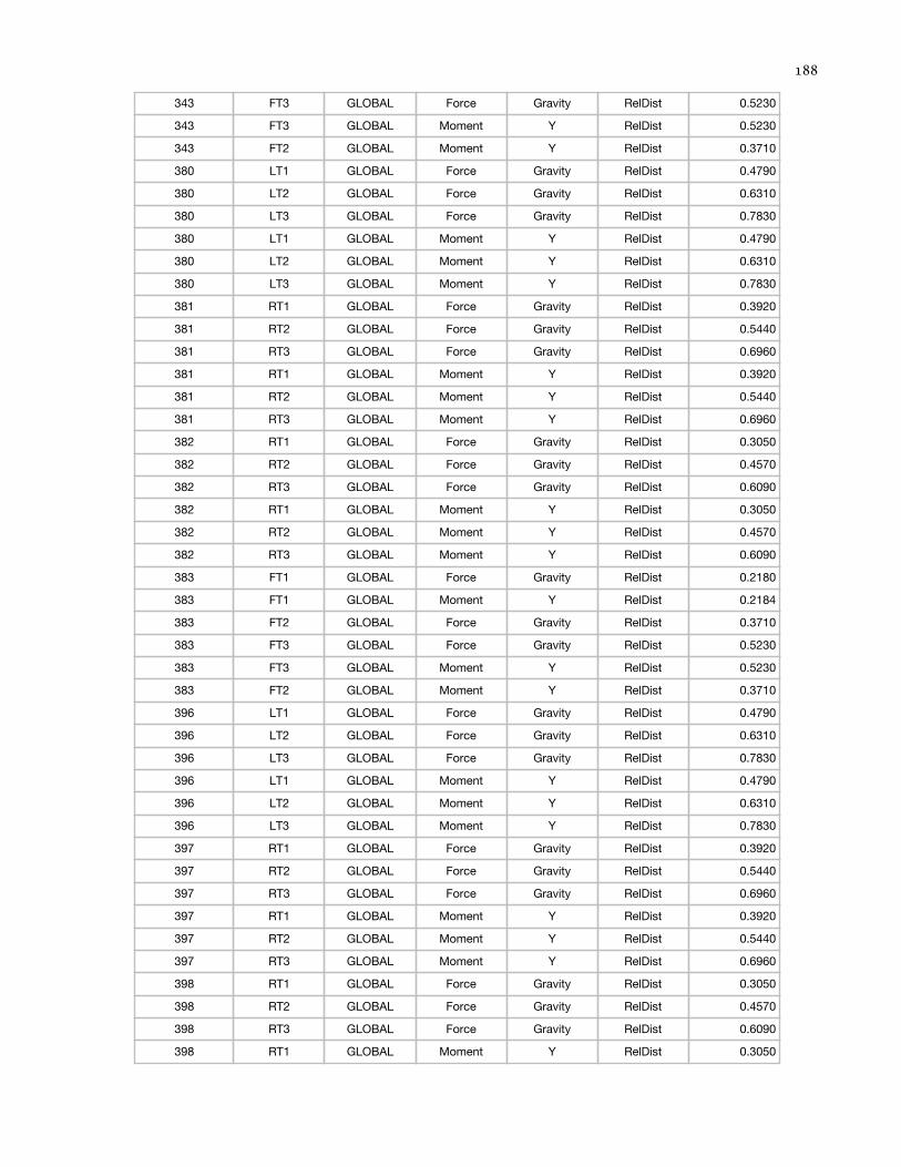
343 FT3 GLOBAL Force Gravity RelDist 0.5230
343 FT3 GLOBAL Moment Y RelDist 0.5230
343 FT2 GLOBAL Moment Y RelDist 0.3710
380 LT1 GLOBAL Force Gravity RelDist 0.4790
380 LT2 GLOBAL Force Gravity RelDist 0.6310
380 LT3 GLOBAL Force Gravity RelDist 0.7830
380 LT1 GLOBAL Moment Y RelDist 0.4790
380 LT2 GLOBAL Moment Y RelDist 0.6310
380 LT3 GLOBAL Moment Y RelDist 0.7830
381 RT1 GLOBAL Force Gravity RelDist 0.3920
381 RT2 GLOBAL Force Gravity RelDist 0.5440
381 RT3 GLOBAL Force Gravity RelDist 0.6960
381 RT1 GLOBAL Moment Y RelDist 0.3920
381 RT2 GLOBAL Moment Y RelDist 0.5440
381 RT3 GLOBAL Moment Y RelDist 0.6960
382 RT1 GLOBAL Force Gravity RelDist 0.3050
382 RT2 GLOBAL Force Gravity RelDist 0.4570
382 RT3 GLOBAL Force Gravity RelDist 0.6090
382 RT1 GLOBAL Moment Y RelDist 0.3050
382 RT2 GLOBAL Moment Y RelDist 0.4570
382 RT3 GLOBAL Moment Y RelDist 0.6090
383 FT1 GLOBAL Force Gravity RelDist 0.2180
383 FT1 GLOBAL Moment Y RelDist 0.2184
383 FT2 GLOBAL Force Gravity RelDist 0.3710
383 FT3 GLOBAL Force Gravity RelDist 0.5230
383 FT3 GLOBAL Moment Y RelDist 0.5230
383 FT2 GLOBAL Moment Y RelDist 0.3710
396 LT1 GLOBAL Force Gravity RelDist 0.4790
396 LT2 GLOBAL Force Gravity RelDist 0.6310
396 LT3 GLOBAL Force Gravity RelDist 0.7830
396 LT1 GLOBAL Moment Y RelDist 0.4790
396 LT2 GLOBAL Moment Y RelDist 0.6310
396 LT3 GLOBAL Moment Y RelDist 0.7830
397 RT1 GLOBAL Force Gravity RelDist 0.3920
397 RT2 GLOBAL Force Gravity RelDist 0.5440
397 RT3 GLOBAL Force Gravity RelDist 0.6960
397 RT1 GLOBAL Moment Y RelDist 0.3920
397 RT2 GLOBAL Moment Y RelDist 0.5440
397 RT3 GLOBAL Moment Y RelDist 0.6960
398 RT1 GLOBAL Force Gravity RelDist 0.3050
398 RT2 GLOBAL Force Gravity RelDist 0.4570
398 RT3 GLOBAL Force Gravity RelDist 0.6090
398 RT1 GLOBAL Moment Y RelDist 0.3050
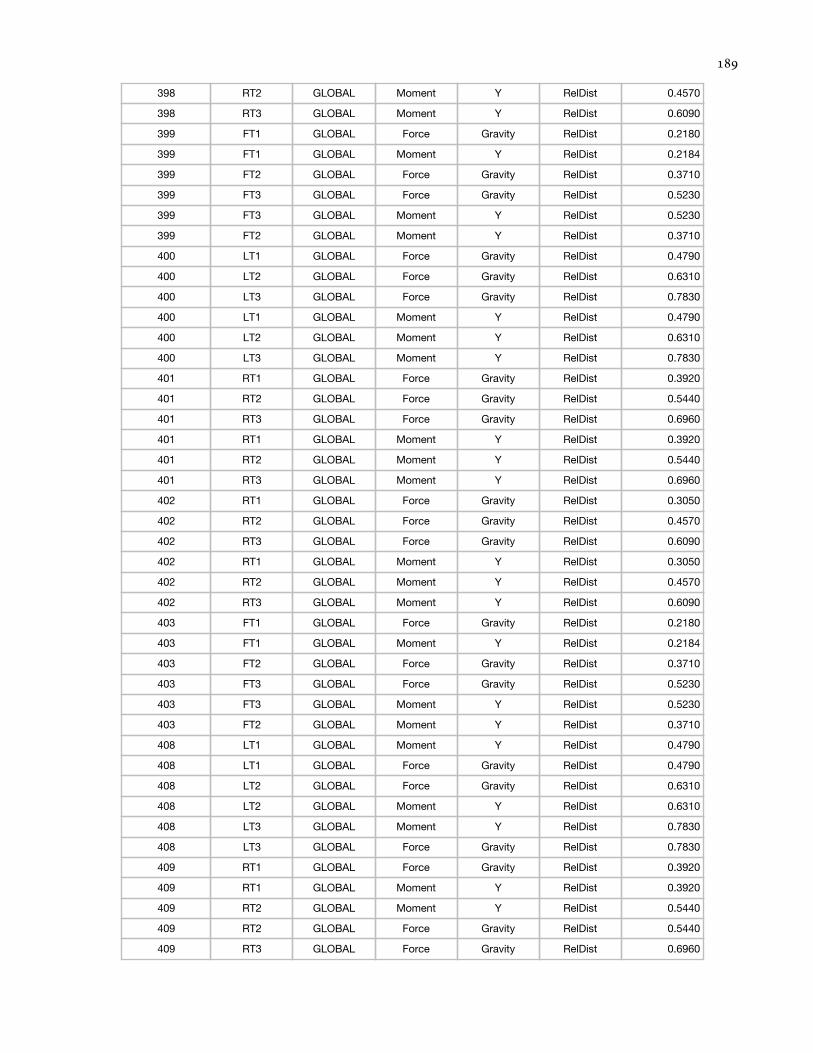
398 RT2 GLOBAL Moment Y RelDist 0.4570
398 RT3 GLOBAL Moment Y RelDist 0.6090
399 FT1 GLOBAL Force Gravity RelDist 0.2180
399 FT1 GLOBAL Moment Y RelDist 0.2184
399 FT2 GLOBAL Force Gravity RelDist 0.3710
399 FT3 GLOBAL Force Gravity RelDist 0.5230
399 FT3 GLOBAL Moment Y RelDist 0.5230
399 FT2 GLOBAL Moment Y RelDist 0.3710
400 LT1 GLOBAL Force Gravity RelDist 0.4790
400 LT2 GLOBAL Force Gravity RelDist 0.6310
400 LT3 GLOBAL Force Gravity RelDist 0.7830
400 LT1 GLOBAL Moment Y RelDist 0.4790
400 LT2 GLOBAL Moment Y RelDist 0.6310
400 LT3 GLOBAL Moment Y RelDist 0.7830
401 RT1 GLOBAL Force Gravity RelDist 0.3920
401 RT2 GLOBAL Force Gravity RelDist 0.5440
401 RT3 GLOBAL Force Gravity RelDist 0.6960
401 RT1 GLOBAL Moment Y RelDist 0.3920
401 RT2 GLOBAL Moment Y RelDist 0.5440
401 RT3 GLOBAL Moment Y RelDist 0.6960
402 RT1 GLOBAL Force Gravity RelDist 0.3050
402 RT2 GLOBAL Force Gravity RelDist 0.4570
402 RT3 GLOBAL Force Gravity RelDist 0.6090
402 RT1 GLOBAL Moment Y RelDist 0.3050
402 RT2 GLOBAL Moment Y RelDist 0.4570
402 RT3 GLOBAL Moment Y RelDist 0.6090
403 FT1 GLOBAL Force Gravity RelDist 0.2180
403 FT1 GLOBAL Moment Y RelDist 0.2184
403 FT2 GLOBAL Force Gravity RelDist 0.3710
403 FT3 GLOBAL Force Gravity RelDist 0.5230
403 FT3 GLOBAL Moment Y RelDist 0.5230
403 FT2 GLOBAL Moment Y RelDist 0.3710
408 LT1 GLOBAL Moment Y RelDist 0.4790
408 LT1 GLOBAL Force Gravity RelDist 0.4790
408 LT2 GLOBAL Force Gravity RelDist 0.6310
408 LT2 GLOBAL Moment Y RelDist 0.6310
408 LT3 GLOBAL Moment Y RelDist 0.7830
408 LT3 GLOBAL Force Gravity RelDist 0.7830
409 RT1 GLOBAL Force Gravity RelDist 0.3920
409 RT1 GLOBAL Moment Y RelDist 0.3920
409 RT2 GLOBAL Moment Y RelDist 0.5440
409 RT2 GLOBAL Force Gravity RelDist 0.5440
409 RT3 GLOBAL Force Gravity RelDist 0.6960

409 RT3 GLOBAL Moment Y RelDist 0.6960
410 RT1 GLOBAL Force Gravity RelDist 0.3050
410 RT1 GLOBAL Moment Y RelDist 0.3050
410 RT2 GLOBAL Moment Y RelDist 0.4570
410 RT2 GLOBAL Force Gravity RelDist 0.4570
410 RT3 GLOBAL Force Gravity RelDist 0.6090
410 RT3 GLOBAL Moment Y RelDist 0.6090
411 FT1 GLOBAL Force Gravity RelDist 0.2180
411 FT1 GLOBAL Moment Y RelDist 0.2184
411 FT2 GLOBAL Force Gravity RelDist 0.3710
411 FT3 GLOBAL Force Gravity RelDist 0.5230
411 FT3 GLOBAL Moment Y RelDist 0.5230
411 FT2 GLOBAL Moment Y RelDist 0.3710
Table: Frame Loads - Point, Part 2 of 2
Frame LoadCase AbsDist Force Moment GUID
Text Text mm KN KN-mm Text
43 LT1 1113.62 75.000
43 LT2 1415.18 75.000
43 LT3 1714.77 75.000
43 LT1 1113.62 -24000.00
43 LT2 1415.18 -24000.00
43 LT3 1714.77 -24000.00
45 FT1 260.17 75.000
45 FT1 260.17 -24000.00
45 FT2 559.76 75.000
45 FT3 859.36 75.000
45 FT3 859.36 -24000.00
45 FT2 559.76 -24000.00
73 LT1 1113.62 87.500
73 LT2 1415.18 87.500
73 LT3 1714.77 87.500
73 LT1 1113.62 16000.00
73 LT2 1415.18 16000.00
73 LT3 1714.77 16000.00
75 FT1 260.17 87.500
75 FT1 260.17 16000.00
75 FT2 559.76 87.500
75 FT3 859.36 87.500
75 FT3 859.36 16000.00
75 FT2 559.76 16000.00
85 LT1 1113.62 62.500
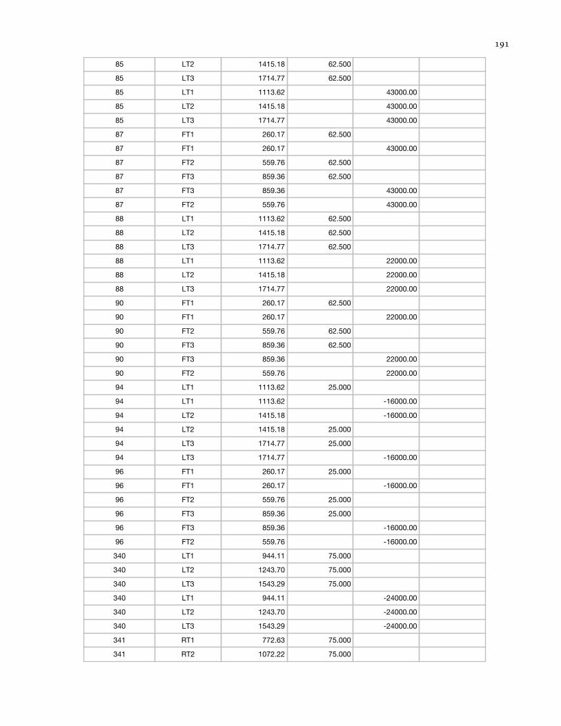
85 LT2 1415.18 62.500
85 LT3 1714.77 62.500
85 LT1 1113.62 43000.00
85 LT2 1415.18 43000.00
85 LT3 1714.77 43000.00
87 FT1 260.17 62.500
87 FT1 260.17 43000.00
87 FT2 559.76 62.500
87 FT3 859.36 62.500
87 FT3 859.36 43000.00
87 FT2 559.76 43000.00
88 LT1 1113.62 62.500
88 LT2 1415.18 62.500
88 LT3 1714.77 62.500
88 LT1 1113.62 22000.00
88 LT2 1415.18 22000.00
88 LT3 1714.77 22000.00
90 FT1 260.17 62.500
90 FT1 260.17 22000.00
90 FT2 559.76 62.500
90 FT3 859.36 62.500
90 FT3 859.36 22000.00
90 FT2 559.76 22000.00
94 LT1 1113.62 25.000
94 LT1 1113.62 -16000.00
94 LT2 1415.18 -16000.00
94 LT2 1415.18 25.000
94 LT3 1714.77 25.000
94 LT3 1714.77 -16000.00
96 FT1 260.17 25.000
96 FT1 260.17 -16000.00
96 FT2 559.76 25.000
96 FT3 859.36 25.000
96 FT3 859.36 -16000.00
96 FT2 559.76 -16000.00
340 LT1 944.11 75.000
340 LT2 1243.70 75.000
340 LT3 1543.29 75.000
340 LT1 944.11 -24000.00
340 LT2 1243.70 -24000.00
340 LT3 1543.29 -24000.00
341 RT1 772.63 75.000
341 RT2 1072.22 75.000
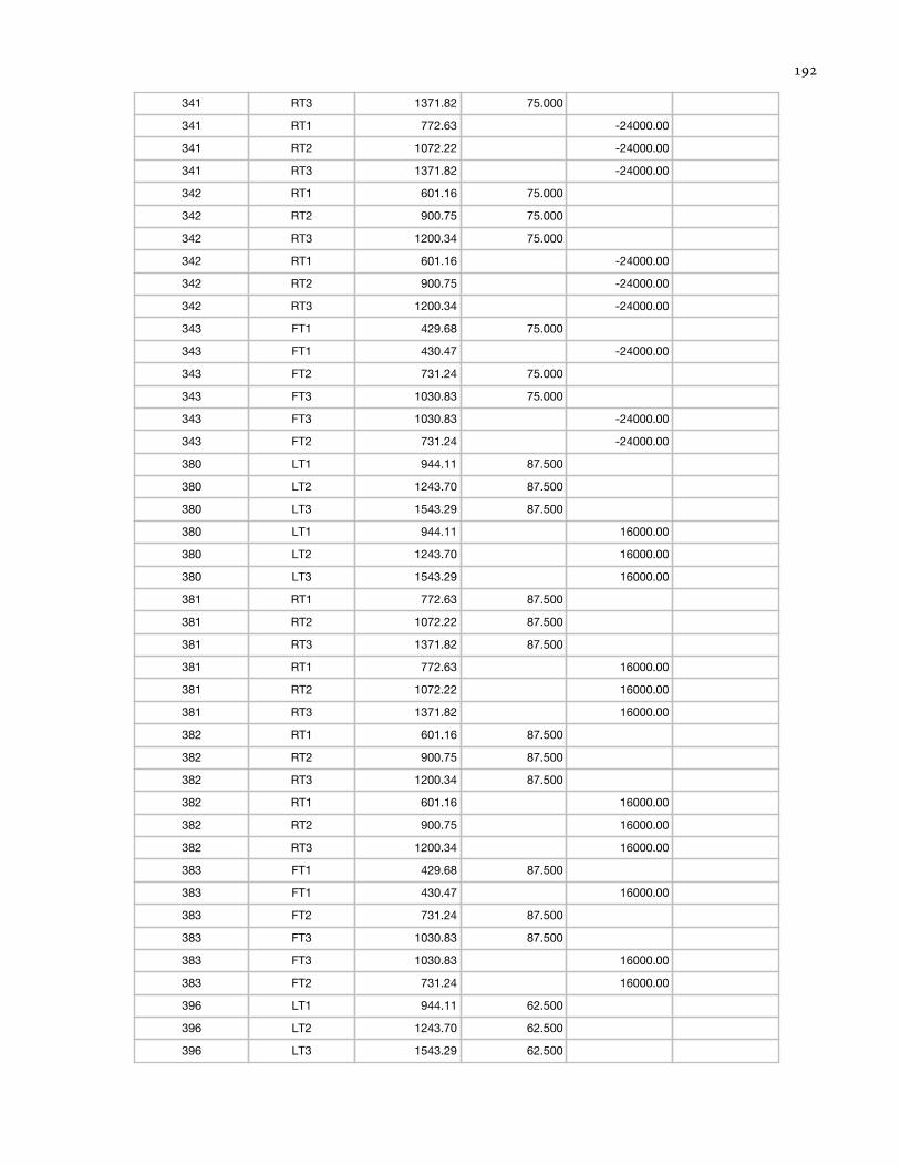
341 RT3 1371.82 75.000
341 RT1 772.63 -24000.00
341 RT2 1072.22 -24000.00
341 RT3 1371.82 -24000.00
342 RT1 601.16 75.000
342 RT2 900.75 75.000
342 RT3 1200.34 75.000
342 RT1 601.16 -24000.00
342 RT2 900.75 -24000.00
342 RT3 1200.34 -24000.00
343 FT1 429.68 75.000
343 FT1 430.47 -24000.00
343 FT2 731.24 75.000
343 FT3 1030.83 75.000
343 FT3 1030.83 -24000.00
343 FT2 731.24 -24000.00
380 LT1 944.11 87.500
380 LT2 1243.70 87.500
380 LT3 1543.29 87.500
380 LT1 944.11 16000.00
380 LT2 1243.70 16000.00
380 LT3 1543.29 16000.00
381 RT1 772.63 87.500
381 RT2 1072.22 87.500
381 RT3 1371.82 87.500
381 RT1 772.63 16000.00
381 RT2 1072.22 16000.00
381 RT3 1371.82 16000.00
382 RT1 601.16 87.500
382 RT2 900.75 87.500
382 RT3 1200.34 87.500
382 RT1 601.16 16000.00
382 RT2 900.75 16000.00
382 RT3 1200.34 16000.00
383 FT1 429.68 87.500
383 FT1 430.47 16000.00
383 FT2 731.24 87.500
383 FT3 1030.83 87.500
383 FT3 1030.83 16000.00
383 FT2 731.24 16000.00
396 LT1 944.11 62.500
396 LT2 1243.70 62.500
396 LT3 1543.29 62.500
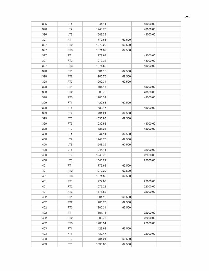
396 LT1 944.11 43000.00
396 LT2 1243.70 43000.00
396 LT3 1543.29 43000.00
397 RT1 772.63 62.500
397 RT2 1072.22 62.500
397 RT3 1371.82 62.500
397 RT1 772.63 43000.00
397 RT2 1072.22 43000.00
397 RT3 1371.82 43000.00
398 RT1 601.16 62.500
398 RT2 900.75 62.500
398 RT3 1200.34 62.500
398 RT1 601.16 43000.00
398 RT2 900.75 43000.00
398 RT3 1200.34 43000.00
399 FT1 429.68 62.500
399 FT1 430.47 43000.00
399 FT2 731.24 62.500
399 FT3 1030.83 62.500
399 FT3 1030.83 43000.00
399 FT2 731.24 43000.00
400 LT1 944.11 62.500
400 LT2 1243.70 62.500
400 LT3 1543.29 62.500
400 LT1 944.11 22000.00
400 LT2 1243.70 22000.00
400 LT3 1543.29 22000.00
401 RT1 772.63 62.500
401 RT2 1072.22 62.500
401 RT3 1371.82 62.500
401 RT1 772.63 22000.00
401 RT2 1072.22 22000.00
401 RT3 1371.82 22000.00
402 RT1 601.16 62.500
402 RT2 900.75 62.500
402 RT3 1200.34 62.500
402 RT1 601.16 22000.00
402 RT2 900.75 22000.00
402 RT3 1200.34 22000.00
403 FT1 429.68 62.500
403 FT1 430.47 22000.00
403 FT2 731.24 62.500
403 FT3 1030.83 62.500
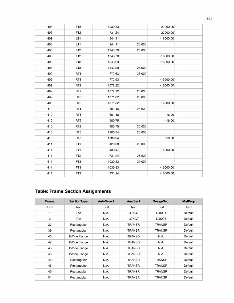
403 FT3 1030.83 22000.00
403 FT2 731.24 22000.00
408 LT1 944.11 -16000.00
408 LT1 944.11 25.000
408 LT2 1243.70 25.000
408 LT2 1243.70 -16000.00
408 LT3 1543.29 -16000.00
408 LT3 1543.29 25.000
409 RT1 772.63 25.000
409 RT1 772.63 -16000.00
409 RT2 1072.22 -16000.00
409 RT2 1072.22 25.000
409 RT3 1371.82 25.000
409 RT3 1371.82 -16000.00
410 RT1 601.16 25.000
410 RT1 601.16 -16.00
410 RT2 900.75 -16.00
410 RT2 900.75 25.000
410 RT3 1200.34 25.000
410 RT3 1200.34 -16.00
411 FT1 429.68 25.000
411 FT1 430.47 -16000.00
411 FT2 731.24 25.000
411 FT3 1030.83 25.000
411 FT3 1030.83 -16000.00
411 FT2 731.24 -16000.00
Table: Frame Section Assignments
Frame SectionType AutoSelect AnalSect DesignSect MatProp
Text Text Text Text Text Text
1 Tee N.A. LONGT LONGT Default
2 Tee N.A. LONGT LONGT Default
37 Rectangular N.A. TRANSR TRANSR Default
39 Rectangular N.A. TRANSR TRANSR Default
40 I/Wide Flange N.A. TRANSD N.A. Default
42 I/Wide Flange N.A. TRANSD N.A. Default
43 I/Wide Flange N.A. TRANSD N.A. Default
45 I/Wide Flange N.A. TRANSD N.A. Default
46 Rectangular N.A. TRANSR TRANSR Default
48 Rectangular N.A. TRANSR TRANSR Default
49 Rectangular N.A. TRANSR TRANSR Default
51 Rectangular N.A. TRANSR TRANSR Default

52 Rectangular N.A. TRANSR TRANSR Default
54 Rectangular N.A. TRANSR TRANSR Default
55 Rectangular N.A. TRANSR TRANSR Default
57 Rectangular N.A. TRANSR TRANSR Default
58 Rectangular N.A. TRANSR TRANSR Default
60 Rectangular N.A. TRANSR TRANSR Default
61 Rectangular N.A. TRANSR TRANSR Default
63 Rectangular N.A. TRANSR TRANSR Default
64 Rectangular N.A. TRANSR TRANSR Default
66 Rectangular N.A. TRANSR TRANSR Default
67 Rectangular N.A. TRANSR TRANSR Default
69 Rectangular N.A. TRANSR TRANSR Default
70 Rectangular N.A. TRANSR TRANSR Default
72 Rectangular N.A. TRANSR TRANSR Default
73 Rectangular N.A. TRANSR TRANSR Default
75 Rectangular N.A. TRANSR TRANSR Default
76 Rectangular N.A. TRANSR TRANSR Default
78 Rectangular N.A. TRANSR TRANSR Default
79 Rectangular N.A. TRANSR TRANSR Default
81 Rectangular N.A. TRANSR TRANSR Default
82 Rectangular N.A. TRANSR TRANSR Default
84 Rectangular N.A. TRANSR TRANSR Default
85 Rectangular N.A. TRANSR TRANSR Default
87 Rectangular N.A. TRANSR TRANSR Default
88 Rectangular N.A. TRANSR TRANSR Default
90 Rectangular N.A. TRANSR TRANSR Default
91 Rectangular N.A. TRANSR TRANSR Default
93 Rectangular N.A. TRANSR TRANSR Default
94 Rectangular N.A. TRANSR TRANSR Default
96 Rectangular N.A. TRANSR TRANSR Default
97 Rectangular N.A. TRANSR TRANSR Default
99 Rectangular N.A. TRANSR TRANSR Default
100 Rectangular N.A. TRANSR TRANSR Default
102 Rectangular N.A. TRANSR TRANSR Default
103 Rectangular N.A. TRANSR TRANSR Default
105 Rectangular N.A. TRANSR TRANSR Default
152 Rectangular N.A. LONGR LONGR Default
176 Rectangular N.A. LONGR LONGR Default
200 Rectangular N.A. LONGR LONGR Default
224 Rectangular N.A. LONGR LONGR Default
248 Rectangular N.A. LONGR LONGR Default
272 Tee N.A. TRANSE TRANSE Default
273 Tee N.A. TRANSE TRANSE Default

274 Tee N.A. TRANSE TRANSE Default
275 Tee N.A. TRANSE TRANSE Default
276 Tee N.A. TRANSE TRANSE Default
277 Tee N.A. TRANSE TRANSE Default
278 Tee N.A. TRANSE TRANSE Default
279 Tee N.A. TRANSE TRANSE Default
280 Tee N.A. TRANSE TRANSE Default
281 Tee N.A. TRANSE TRANSE Default
282 Tee N.A. TRANSE TRANSE Default
283 Tee N.A. TRANSE TRANSE Default
332 Rectangular N.A. TRANSR TRANSR Default
333 Rectangular N.A. TRANSR TRANSR Default
334 Rectangular N.A. TRANSR TRANSR Default
335 Rectangular N.A. TRANSR TRANSR Default
336 I/Wide Flange N.A. TRANSD N.A. Default
337 I/Wide Flange N.A. TRANSD N.A. Default
338 I/Wide Flange N.A. TRANSD N.A. Default
339 I/Wide Flange N.A. TRANSD N.A. Default
340 I/Wide Flange N.A. TRANSD N.A. Default
341 I/Wide Flange N.A. TRANSD N.A. Default
342 I/Wide Flange N.A. TRANSD N.A. Default
343 I/Wide Flange N.A. TRANSD N.A. Default
344 Rectangular N.A. TRANSR TRANSR Default
345 Rectangular N.A. TRANSR TRANSR Default
346 Rectangular N.A. TRANSR TRANSR Default
347 Rectangular N.A. TRANSR TRANSR Default
348 Rectangular N.A. TRANSR TRANSR Default
349 Rectangular N.A. TRANSR TRANSR Default
350 Rectangular N.A. TRANSR TRANSR Default
351 Rectangular N.A. TRANSR TRANSR Default
352 Rectangular N.A. TRANSR TRANSR Default
353 Rectangular N.A. TRANSR TRANSR Default
354 Rectangular N.A. TRANSR TRANSR Default
355 Rectangular N.A. TRANSR TRANSR Default
356 Rectangular N.A. TRANSR TRANSR Default
357 Rectangular N.A. TRANSR TRANSR Default
358 Rectangular N.A. TRANSR TRANSR Default
359 Rectangular N.A. TRANSR TRANSR Default
360 Rectangular N.A. TRANSR TRANSR Default
361 Rectangular N.A. TRANSR TRANSR Default
362 Rectangular N.A. TRANSR TRANSR Default
363 Rectangular N.A. TRANSR TRANSR Default
364 Rectangular N.A. TRANSR TRANSR Default

365 Rectangular N.A. TRANSR TRANSR Default
366 Rectangular N.A. TRANSR TRANSR Default
367 Rectangular N.A. TRANSR TRANSR Default
368 Rectangular N.A. TRANSR TRANSR Default
369 Rectangular N.A. TRANSR TRANSR Default
370 Rectangular N.A. TRANSR TRANSR Default
371 Rectangular N.A. TRANSR TRANSR Default
372 Rectangular N.A. TRANSR TRANSR Default
373 Rectangular N.A. TRANSR TRANSR Default
374 Rectangular N.A. TRANSR TRANSR Default
375 Rectangular N.A. TRANSR TRANSR Default
376 Rectangular N.A. TRANSR TRANSR Default
377 Rectangular N.A. TRANSR TRANSR Default
378 Rectangular N.A. TRANSR TRANSR Default
379 Rectangular N.A. TRANSR TRANSR Default
380 Rectangular N.A. TRANSR TRANSR Default
381 Rectangular N.A. TRANSR TRANSR Default
382 Rectangular N.A. TRANSR TRANSR Default
383 Rectangular N.A. TRANSR TRANSR Default
384 Rectangular N.A. TRANSR TRANSR Default
385 Rectangular N.A. TRANSR TRANSR Default
386 Rectangular N.A. TRANSR TRANSR Default
387 Rectangular N.A. TRANSR TRANSR Default
388 Rectangular N.A. TRANSR TRANSR Default
389 Rectangular N.A. TRANSR TRANSR Default
390 Rectangular N.A. TRANSR TRANSR Default
391 Rectangular N.A. TRANSR TRANSR Default
392 Rectangular N.A. TRANSR TRANSR Default
393 Rectangular N.A. TRANSR TRANSR Default
394 Rectangular N.A. TRANSR TRANSR Default
395 Rectangular N.A. TRANSR TRANSR Default
396 Rectangular N.A. TRANSR TRANSR Default
397 Rectangular N.A. TRANSR TRANSR Default
398 Rectangular N.A. TRANSR TRANSR Default
399 Rectangular N.A. TRANSR TRANSR Default
400 Rectangular N.A. TRANSR TRANSR Default
401 Rectangular N.A. TRANSR TRANSR Default
402 Rectangular N.A. TRANSR TRANSR Default
403 Rectangular N.A. TRANSR TRANSR Default
404 Rectangular N.A. TRANSR TRANSR Default
405 Rectangular N.A. TRANSR TRANSR Default
406 Rectangular N.A. TRANSR TRANSR Default
407 Rectangular N.A. TRANSR TRANSR Default

408 Rectangular N.A. TRANSR TRANSR Default
409 Rectangular N.A. TRANSR TRANSR Default
410 Rectangular N.A. TRANSR TRANSR Default
411 Rectangular N.A. TRANSR TRANSR Default
412 Rectangular N.A. TRANSR TRANSR Default
413 Rectangular N.A. TRANSR TRANSR Default
414 Rectangular N.A. TRANSR TRANSR Default
415 Rectangular N.A. TRANSR TRANSR Default
416 Rectangular N.A. TRANSR TRANSR Default
417 Rectangular N.A. TRANSR TRANSR Default
418 Rectangular N.A. TRANSR TRANSR Default
419 Rectangular N.A. TRANSR TRANSR Default
420 Rectangular N.A. TRANSR TRANSR Default
421 Rectangular N.A. TRANSR TRANSR Default
422 Rectangular N.A. TRANSR TRANSR Default
423 Rectangular N.A. TRANSR TRANSR Default
Table: Frame Section Properties 01 - General, Part 1 of 6
SectionName Material Shape t3 t2 tf tw
Text Text Text mm mm mm mm
FSEC1 A992Fy50 Rectangular 500.000 300.000
LONGR CONC Rectangular 225.000 1971.000
LONGT CONC Tee 2000.000 1971.000 343.500 297.500
LONGTD CONC Tee 1172.000 1971.000 343.500 303.750
TRANSD CONC I/Wide Flange 2000.000 1525.000 273.000 300.000
TRANSE CONC Tee 2000.000 1525.000 273.000 600.000
TRANSR CONC Rectangular 273.000 1525.000
Table: Frame Section Properties 01 - General, Part 2 of 6
SectionName t2b tfb Area TorsConst I33 I22 AS2
Text mm mm mm2 mm4 mm4 mm4 mm2
FSEC1 150000.00 2817370800 3125000000 1125000000 125000.00
LONGR 443475.00 6945441210 1870910156 1.436E+11 369562.50
LONGT 1169847.25 3.923E+10 4.046E+11 2.228E+11 595000.00
LONGTD 928695.38 3.240E+10 8.405E+10 2.211E+11 355995.00
TRANSD 1100.000 504.000 1337625.00 5.187E+10 6.854E+11 1.393E+11 600000.00
TRANSE 1452525.00 1.288E+11 5.571E+11 1.118E+11 1200000.00
TRANSR 416325.00 9176401718 2585690494 8.068E+10 346937.50
Table: Frame Section Properties 01 - General, Part 3 of 6

SectionName AS3 S33 S22 Z33 Z22 R33 R22
Text mm2 mm3 mm3 mm3 mm3 mm mm
FSEC1 125000.00 12500000.00 7500000.00 18750000.00 11250000.00 144.338 86.603
LONGR 369562.50 16630312.50 145681537.5 24945468.75 218522306.3 64.952 568.979
LONGT 564198.75 287531576.9 226095347.4 520145212. 370263372. 588.063 436.425
LONGTD 564198.75 99889501.49 224370523.3 197578735.4 352720915. 300.842 487.949
TRANSD 808937.50 678933434. 182738888.3 886427920. 338701406. 715.842 322.751
TRANSE 346937.50 484404742. 146584462.1 791484973. 314153906.3 619.319 277.397
TRANSR 346937.50 18942787.50 105815937.5 28414181.25 158723906.3 78.808 440.230
Table: Frame Section Properties 01 - General, Part 4 of 6
SectionName ConcCol ConcBeam Color TotalWt TotalMass FromFile AMod
Text Yes/No Yes/No Text KN KN-s2/mm Yes/No Unitless
FSEC1 No No Green 0.000 0.000000 No 1.000000
LONGR No Yes Blue 6246.804 0.636997 No 1.000000
LONGT No Yes Red 6591.403 0.672136 No 1.000000
LONGTD No Yes White 0.000 0.000000 No 1.000000
TRANSD No No Cyan 2435.229 0.248324 No 1.000000
TRANSE No Yes Yellow 2644.412 0.269655 No 1.000000
TRANSR No Yes 16744576 7958.428 0.811534 No 1.000000
Table: Program Control, Part 1 of 2
ProgramName Version ProgLevel LicenseOS LicenseSC LicenseBR LicenseHT CurrUnits
Text Text Text Yes/No Yes/No Yes/No Yes/No Text
SAP2000 11.0.8 Advanced No No Yes No KN, mm, C