system identi cation general aspects and structure manfred ... · system identi cation general...

System Identification

General Aspects and Structure

Manfred Deistler

TU - WienInstitut fur Wirtschaftsmathematik,

Arbeitsgruppe Okonometrie & Systemtheorie (EOS)Argentinierstrasse 8

A-1040 Wien

e-mail: [email protected]://www.eos.tuwien.ac.at/Oeko/

Joint ICCoS-IAP Study DayLouvain-la-Neuve

24-03-04

Contents

1. Introduction

2. Structure Theory

3. Estimation for a Given Subclass

4. Model Selection

5. Linear Non-Mainstream Cases

6. Nonlinear Systems

7. Present State and Future Developments

1. Introduction

The art of identification is to find a good model fromnoisy data: Data driven modeling.

This is an important problem in many fields of applica-tion.

Systematic approaches: Statistics, System Theory, Econo-metrics, Inverse Problems.

MAIN STEPS IN IDENTIFICATION

• Specify the model class (i.e. the class of all a pri-ori feasible candidate systems): Incorporation of apriori knowledge.

• Specify class of observations.

• Identification in the narrow sense. An identificationprocedure is a rule (in the automatic case a func-tion) attaching a system from the model class tothe data

– Development of procedures.

– Evaluation of procedures (Statistical and nu-merical properties).

Here only identification from equally spaced, discretetime data yt, t = 1, . . . T ; yt ∈ Rs is considered.

1. Introduction

MAIN PARTS

• Main stream theory for linear systems (Nonlinear!).

• Alternative approaches to linear system identifica-tion.

• Identification of nonlinear systems: parametric, non-parametric

MAINSTREAM THEORY

• The model class consists of linear, time-invariant,finite dimensional, causal and stable systems only.The classification of the variables into inputs andoutputs is given a priori.

• Stochastic models for noise are used; in particularnoise is assumed to be stationary, ergodic with arational spectral density.

• The observed inputs are assumed to be free of noiseand to be uncorrelated with the noise process.

• Semi-nonparametric approach: A parametric sub-class is determined by model selection procedures.First step: Estimation of integer valued parame-ters.Then, for the given subclass, the finite dimensionalvector of real valued parameters is estimated.

1. Introduction

• Emphasis on asymptotic properties (consistency,asymptotic distribution) in evaluation.

3 MODULES IN IDENTIFICATION

• STRUCTURE THEORY: Idealized Problem;we commence from the stochastic processes gener-ating the data (or their population moments) ratherthan from data. Relation between ”external behav-ior” and ”internal parameters”.

• ESTIMATION OF REAL VALUED PARAMETERS:Subclass (dynamic specification) is assumed to begiven and parameter space is a subset of an Eu-clidean space and contains a nonvoid open set: M-estimators

• MODEL SELECTION: In general, the orders, therelevant inputs or even the functional forms are notknown a priori and have to be determined fromdata. In many cases, this corresponds to estimatinga model subclass within the original model class.This is done, e.g. by estimation of integers, e.g.using information criteria or test sequences.

1. Introduction

THE HISTORY OF THE SUBJECT

(i) Early (systematic, methodological) time series anal-ysis dates back to the 18th and 19th century. Mainfocus was the search for “hidden”periodicities andtrends, e.g. in the orbits of planets (Laplace, Eu-ler, Lagrange, Fourier). Periodogram (A. Schus-ter). Economic time series, e.g. for business cycledata.

(ii) Yule (1921, 1923). Linear stochastic systems (MAand AR systems) used for explaining “almost peri-odic” cycles: yt − a1yt−1 − a2yt−2 = εt.

(iii) (Linear) Theory of (weak sense) stationary pro-cesses (Cramer, Kolmogoroff, Wiener, Wold). Spec-tral representation, Wold representation (linear sys-tems), factorization, prediction, filtering and inter-polation.

(iv) Early econometrics, in particular, the work of theCowles Commission (Haavelmo, Koopmans, T. W.Anderson, Rubin, L. Klein). theory of identifiabil-ity and of (Gaussian) Maximum Likelihood (ML)- estimation for (finite dimensional) MIMO (multi-input, multi-output) linear systems (vector differ-ence equations) with white noise errors (ARX sys-tems). The maximum lag lengths are assumed tobe known a priori. Development of LIML, 2SLSand 3 SLS estimators (Theil, Zellner).

1. Introduction

(v) (Nonparametric) Spectral estimation and estima-tion of transfer functions (Tukey).

(vi) Estimation of AR, ARMA, ARX and ARMAX sys-tems. SISO (single-input,single-output) case. Em-phasis on asymptotic normality and efficiency, inparticular, for least squares and ML estimators.(T.W. Anderson, Hannan, Walker).

(vii) Structure theory for (MIMO) state space and ARMAsystems (Kalman).

(viii) Box-Jenkins procedure: An “integrated” approachto SISO system identification including order esti-mation (non automatic), the treatment of certainnon-stationarities and numerically efficient ML al-gorithms. Big impact on applications.

(ix) Automatic procedures for order estimation, in par-ticular, procedures based on information criteria (likeAIC, BIC) (Akaike, Rissanen).

(x) Main stream theory for linear system identification(including MIMO systems): Structure theory, or-der estimation, estimation for “real valued” param-eters with emphasis on asymptotic theory (Hannan,Akaike, Caines, Ljung).

(xi) Alternative approaches.

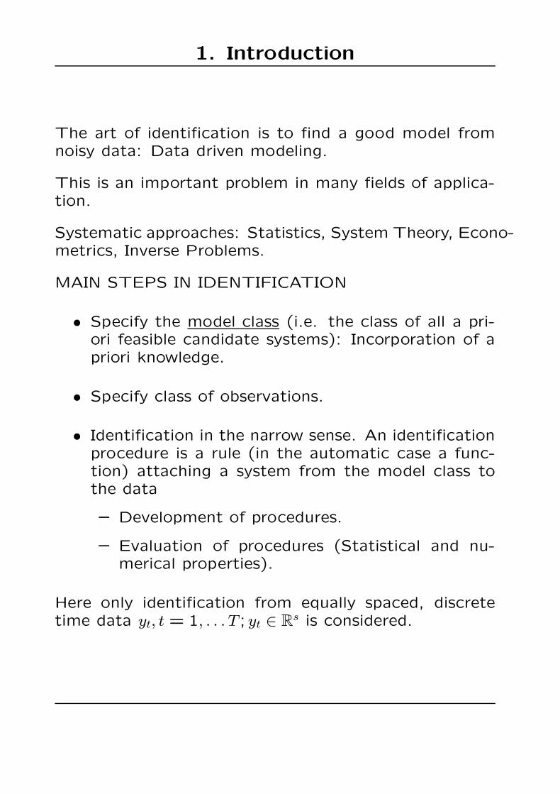
2. Structure Theory

Relation between external behavior and internal param-eters. Linear, main stream case: Relations betweentransfer function and parameters.

Main model classes for linear systems:

• AR(X)

• ARMA(X)

• State Space Models

Here, for simplicity of notation we assume that we haveno observed inputs.

In many applications AR models still dominate.

Advantages of AR models:

• no problems of non-identifiability, structure theoryis simple

• maximum likelihood estimates are of least squarestype, i.e. asymptotically efficient and easy to cal-culate

Disadvantages of AR models:

• less flexible

2. Structure Theory

Here, the focus is on state space models.

State space forms in innovation representation:

xt+1 = Axt + Bεt (1)

yt = Cxt + εt (2)

where

• yt: s-dimensional outputs

• xt: n-dimensional states

• (εt) white noise

• A ∈ Rn×n, B ∈ Rn×s, C ∈ Rs×n: parameter matrices

• n: integer valued parameter

2. Structure Theory

Assumptions:

|λmax(A)| < 1 (3)

|λmax(A−BC)| ≤ 1 (4)

Eεtε′

t = Σ > 0 (5)

Transfer function:

k(z) =

∞∑

j=1

Kjzj + I

Kj = CAj−1B (6)

ARMA forms

a(z)yt = b(z)εt

External behavior

f(λ) = (2π)−1k(e−iλ)Σk∗(e−iλ)f ↔ (k,Σ)

Note that ARMA and state space systems describe thesame class of transfer functions.

2. Structure Theory

Relation to internal parameters:

(6) or a−1b = k

UA = {k| rational, s × s, k(0) = I, no poles for |z| ≤ 1and no zeros for |z| < 1}

M(n) ⊂ UA: Set of all transfer functions of order n.

TA: Set of all A,B,C for fixed s, but n variable, satisfying(4) and (5).

S(n) ⊂ TA: Subset of all (A,B,C) for fixed n.

Sm(n) ⊂ S(n): Subset of all minimal (A,B,C).

π : TA → UA : π(A,B,C) = k = C(Iz−1 − A)−1B + I

π is surjective but not injective

Note: TA is not a good parameter space because:

• TA is infinite dimensional

• lack of identifiability

• lack of ”well posedness”: There exists no contin-uous selection from the equivalence classes π−1(k)for Tα.

2. Structure Theory

2. Structure Theory

Desirable properties of parametrizations:

• UA and TA are broken into bits, Uα and Tα, α ∈ I,such that k restricted to Tα: π|Tα : Tα → Uα is bijec-tive. Then there exists a parametrization ψα : Uα →Tα such that ψα(π(A,B,C)) = (A,B,C) ∀(A,B,C) ∈Tα.

• Uα is finite dimensional in the sense that Uα ⊂∪ni=1M(n) for some n.

• Well posedness: The parametrization ψα : Uα →Tα is a homeomorphism (pointwise topology Tpt forUA).

• Uα is Tpt-open in Uα.

• ∪α∈IUα is a cover for UA.

Examples:

• Canonical forms based on M(n), e.g. echelon formsand balanced realizations. Decomposition of M(n)into sets Uα of different dimension. Nice free pa-rameters vs. nice spaces of free parameters.

• ”Overlapping description” of the manifold M(n) bylocal coordinates.

2. Structure Theory

• ”Full parametrization” for state space systems. HereS(n) ⊂ Rn2+2ns or Sm(n) are used as parameterspaces for M(n) or M(n), respectively. Lack ofidentifiability. The equivalence classes are n2 di-mensional manifolds. The likelihood function isconstant along these classes.

• Data driven local coordinates (DDLC): Orthonormalcoordinates for the 2ns dimensional ortho-complementof the tangent space to the equivalence class at aninitial estimator. Extensions: slsDDLC and orthoDDLC

• ARMA systems with prescribed column degrees.

• ARMA parametrizations commencing from writingk as c−1p where c is a least common denominatorpolynomial for k and where the degrees of c and pserve as integer valued parameters.

In general, state space systems have larger equivalenceclasses compared to ARMA systems: More freedom inselection of optimal representatives.

Main unanswered question: Optimal tradeoff between”number” and dimension of the pieces Uα.

2. Structure Theory

Problem: Numerical properties of parametrizations

Different parametrizations:

ψ1 : U1 → T1 ⊂ TA

ψ2 : U2 → T2 ⊂ TA

For the asymptotic analysis, in the case that U1 ⊃ U2,U2 contains a nonvoid open (in U1) set and k0 ∈ U2, wehave:

STATISTICAL ANALYSIS (”real world”):

• no essential differences: coordinate free consistency

• different asymptotic distributions, but we know thetransformation

NUMERICAL ANALYSIS (”integer world”):

• The selection from the equivalence class matters

• Dependency on algorithm

2. Structure Theory

Questions:

• What are appropriate evaluation criteria for numer-ical properties?

• Which are the optimal parameter spaces (algorithmspecific)?

Relation between statistical and numerical precision: cur-vature of the criterion function:

2. Structure Theory

Consider the case s = n = 1 where (a, b, c) ∈ R3:

• Minimality: b 6= 0 and c 6= 0

• Equivalence classes of minimal systems: a = a, b =tb, c = ct−1, t ∈ R \ {0}

−2

0

2 −10 −5 0 5 10

−8

−6

−4

−2

0

2

4

6

8

B

StabOber for γ=−1

DDLC for initial StabOber

StabOber for γ=1

MinOber for γ=−1

Echelon

A

C

−10 −5 0 5 10−8

−6

−4

−2

0

2

4

6

8

B

C


We here assume that Uα is given.

Identifiable case: ψα : Uα → Tα has the desirable proper-ties.

τ ∈ Tα ⊂ Rdα: vector of free parameters for Uα.

σ ∈ Σ ⊂ Rn(n+1)

2 : free parameters for Σ > 0.

Overall parameter space: Θ = Tα ×Σ.

Many identification procedures, at least asymptotically,commence from the sample second moments of the data

GENERAL FEATURES:

γ(s) = T−1T−s∑

t=1

yt+sy′

t, s ≥ 0

Now, γ can be directly realized as an MA system typically

of order Ts; ˆkT

Identification:

• Projection step (Model reduction). Important forstatistical qualities.

• Realization step.


• M-estimators:

θT = argminLT(θ; y1, . . . , yT)

• Direct procedures: Explicit functions.


GAUSSIAN MAXIMUM LIKELIHOOD:

LT(θ) = T−1log detΓT(θ) + T−1y′(T)ΓT(θ)−1y(T)

where

y(T) = (y′1, . . . , y′T)

′

ΓT(θ) = Ey(T ; θ)y′(T ; θ)

θT = argminθ∈ΘLT(θ)

• No explicit formula for MLE, in general.

• LT(k,Σ) since LT depends on τ only via k: param-eter free approach.

• Boundary points are important.

Whittle likelihood:

LW,T(k, σ) = log detΣ +

(2π)−1

∫ π

−πtr

[(k(e−iλ)Σk∗(e−iλ)

)−1I(λ)

]

dλ

where I(λ) is the periodogram.


EVALUATION:

• Coordinate free consistency: for k0 ∈ Uα and

limT−1∑T−s

t=1 εt+sε′

t = δ0,sΣ0 a.s. for s ≥ 0 we have

kT → k0 a.s. and ΣT → Σ0 a.s.

Consistency proof: basic idea Wald (1949) for i.i.d.case.

Noncompact parameter spaces:

limT→∞ LT(k, σ) = L(k, σ) = log detΣ + (2π)−1

∫ π

−π tr[(k(e−iλ)Σk∗(e−iλ)

)−1 (k0(e

−iλ)Σ0k∗0(e

−iλ))]

dλ

a.s.

(7)

– L has a unique minimum at k0, Σ0.

– (kT , ΣT) enters a compact set, uniform conver-gence in (7).

• Generalized, coordinate free consistency for k0 6∈ Uα,(kT , ΣT) → D a.s D: Set of all best approximantsto k0,Σ0 in Uα ×Σ.

• Consistency in coordinates: ψα(kT) = τT → τ0 =ψα(k0) a.s.


• CLT:

Under

E(εt|Ft−1) = 0

and

E(εtε′t|Ft−1) = Σ0.

√T (τT − τ0)

d−→ N(0, V )

Idea of proof: Cramer (1946) i.i.d. case: Lineariza-tion.

Direct Estimators: IV Methods, subspace methods: Nu-merically faster, in many cases not asymptotically effi-cient.

CALCULATIONS OF ESTIMATES

Usual procedure:consistent initial estimator (e.g. IV or subspace estima-tor)+ one Gauß-Newton step gives an asymptotically effi-cient procedure (e.g. Hannan-Rissanen)

HOWEVER THERE ARE STILL PROBLEMS

• Problem of local minima: “good” initial estimatesare required


• Numerical problems: Optimization over a gridStatistical accuracy may be higher than numericalaccuracyValleys close to equivalence classes correspondingto lower dimensional systems“Intelligent” parametrization may help DDLC’s andextensions:Data driven selection of coordinates from an un-countable number of possibilitiesOnly locally homeomorphic

• “Curse of dimensionality”lower dimensional parametrizations (e.g. reducedrank models)concentration of the likelihood function by a leastsquares step.

4. Model Selection

Automatic vs. nonautomatic procedures.

Information criteria: Formulate tradeoff between fit andcomplexity. Based on e.g. Bayesian arguments, codingtheory . . .

Order estimation (or more general closure nested case):n1 < n2 implies M(n1) ⊂ M(n2) and

dim(M(n1)) <dim(M(n1)).

Criteria of the form

A(n) = log detΣT(n) + 2ns · c(T) · T−1

where ΣT(n) is the MLE for Σ0 over M(n)×Σ.

c(T) = 2: AIC criterion

c(T) = c·logT, c ≥ 1: BIC criterion

Estimator: nT =argminA(n)

Statistical evaluation: nT is consistent for

limT→∞

c(T)

T= 0, lim inf

T→∞

c(T)

logT> 0

Evaluation of uncertainty coming from model selectionfor estimators of real valued parameters.

4. Model Selection

Note: Complexity is in the eye of the beholder. Considere.g. AR models for s = 1:

yt + a1yt−1 + a2yt−2 = εt

Parameter spaces:

T = {(a1, a2) ∈ R2|1 + a1z+ a2z2 6= 0 for |z| ≤ 1}

T0 = {(0,0)}

T1 = {(a1,0)||a1| < 1, a1 6= 0}

T2 = T − (T0 ∪ T1)

4. Model Selection

Bayesian justification:

• Positive priors for all classes, otherwise MLE is asymp-totically normal

• Certain properties of Uα, α ∈ I are needed, e.g. forBIC to give consistent estimators: closure nested-ness, e.g. n1 > n2 ⇒M(n1) ⊃M(n2)

Main open question:

• Optimal tradeoff between dimension and ”number”of pieces.

4. Model Selection

Problem: Properties of post model selection estimators

• The statistical analysis of the MLE τT traditionallydoes not take into account the additional uncer-tainty coming from model selection.

• This may result in very misleading conclusions

Consider AR case (nested):

yt = a1yt−1 + · · ·+ apyt−p + εt

where

Tp =

a1...ap

∈ Rp|stability

The estimator (LS) for given p is

τp =(X(p)′X(p)

)−1X(p)y

4. Model Selection

The post model selection estimator is

τ =

0...0

1{p=0}+

a1(1)...0

1{p=1}+· · ·+

a1(p)...

ap(p)

1{p=p}

Main problem:

• Essential lack of uniformity in convergence of finitesample distributions.

5. Linear non-mainstream cases

• Time varying parameters

• Unstable systems, integration and cointegration

• Errors in variables, dynamic factor models, identifi-cation in closed loop

COINTEGRATION:

A stochastic process is called integrated (of order 1) if(1− z)yt is stationary, while (yt) is not.

An integrated vector process (yt) is called cointegrated

if ∃α ∈ Rs such that (α′yt) is stationary.

Motivation:

• Trends in means and variance

• α describes long run equilibrium


STRUCTURE THEORY, AR CASE

a(z)yt = εt

SPECIAL REPRESENTATION (Johansen)

(1−z)yt = Γ1(1−z)yt−1+· · ·+Γp−1(1−z)yt−p+1+πyt−p+εt

where π = −a(1) and

rk(π) = s ⇔ (yt) is stationary

rk(π) = 0 ⇔ (yt) is integrated, but not cointegrated

rk(π) = r︸︷︷︸

0<r<s

⇔ (yt) is cointegrated with r l.i. c. v.

π = BA′, A,B ∈ Rs×r. The rows of A span the cointe-grating space.

MLE, AR CASE

• (Gaussian) likelihood LT(Γ1, . . . ,Γp−1,Σ, B,A)

• Concentrated likelihood (stepwise) LT(A, r): likeli-hood ratio tests

– H0: at most r (r < s) l.i. cointegrating vectors

– H1: r+ 1 l.i. cointegrating vectors


• Nonstandard limiting distributions for the test underH0

• Asymptotic properties for the MLE’s AT and BTunder additional normalization: non-normal limitingdistributions, different speeds of convergence.

Simplest case: AR(1), scalar

yt = ρyt−1 + εt

OLS estimate ρT :

√T (ρT − ρ) →d N(0,1− ρ2) for |ρ| < 1

T(ρT − 1) →d

12(W(1)2 − 1)∫ 1

0W(r)2dr

for ρ = 1

where W(.) is the standard Brownian motion; functionalCLT’s and continuous mapping theorem.

• LR tests and MLE’s are available

• Open problems in structure theory and specification

6. Nonlinear systems

Nonlinear system identification is a word like ”non-elephantzoology”

• Asymptotic theory for M-estimation in parametricclasses of nonlinear (dynamic) systems.

• Nonparametric estimation for nonlinear time seriesmodels, e.g. by kernel methods. Nonlinear autore-gression systems yt = g(yt−1, . . . , yt−p) + εt. Asymp-totic theory, rates of convergence.

• Semi-nonparametric estimation, e.g. by dynamicneural nets. ”Universal approximation properties”(nonlinear black box models).

• Special classes of nonlinear systems, e.g. GARCHtype models.

• Chaos models: nonlinearity instead of stochasticity.


ARCH and GARCH models

ARCH:

εt = σtzt

σ2t = c+

p∑

i=1

αiε2t−i

where zt is IID with Ezt = 0 and Ez2t = 1, c > 0, αi ≥ 0.

Stationarity condition:∑p

i=1αi < 1.

Note that (εt) is white noise but E(ε2t |εt−1, εt−2, . . . ) =c+ α1ε

2t−1 + · · ·+ αpε

2t−p

Volatility clustering:


GARCH:

εt = σtzt

σ2t = c+

p∑

i=1

αiε2t−i +

p∑

i=1

βiσ2t−i

where, in addition, β(z) = 1 −∑p

i=1 βizi 6= 0 for |z| ≤ 1

and βi ≥ 0.

Stationarity condition: (α1 + β1) + . . . (αp + βp) < 1

7. Present State and Future

Developments

PRESENT STATE:

• Theory and methods have reached a certain stateof maturity. Large body of methods and theoriesavailable.Identification and control.Demand pull rather than theory push.Increasing fragmentation corresponding to differentfields of application (date structure, model classes,prior knowledge).

• Boom in applications: Number of applications andareas of application are increasing.

Data compression & codingSignal extractionAnalysisForecastingSimulationMonitoringControlEstimation of “physically”

meaningful parametersEmpirical discrimination

between conflictingtheories

Signal processingProcess modeling& control inengineering

FinanceBusiness& Marketing

System biologyMonitoring inmedicine

. . .

“Component manufacturing”Enabling technology, not very visible


Developments

• Different communities and multicultural:

EconometricsStatisticsSystems & ControlSignal processingIntruders, e.g. neural netsShifting boundaries

IMPORTANT PROBLEMS FOR THE FUTURE

• There are still major open problems in linear sys-tems identification

• Highly structured systems, e.g. compartment mod-els

• Nonlinear systems

• Spatio-temporal systems, PDE’s

• Further automatization

• Hybrid procedures

• Use of symbolic computation


Developments

CHANCES AND DANGERS

The increasing number of applications poses challenges.

Will there be still a common body of theory and meth-ods?

Danger of fragmentation and of becoming selfreferen-tial.

system identi cation general aspects and structure manfred ... · system identi cation general...

Documents